The Emergent Behaviour of Thermal Networks and Its Impact on the Thermal Conductivity of Heterogeneous Materials and Systems

Abstract

The properties of thermal networks are examined to understand the effective thermal conductivity of heterogeneous two-phase composite materials and systems. At conditions of high contrast in thermal conductivity of the individual phases (k₁ and k₂), where k₁ << k₂ or k₁ >> k₂, the effective thermal conductivity of individual networks of the same composition was seen to be highly sensitive to the distribution of the phases and the presence of percolation paths across the network. However, when the contrast in thermal conductivities of the two phases was modest (k₁/k₂ ~ 10⁻² to 10²), the thermal networks were observed to exhibit an emergent response with a low variability in the effective thermal conductivity of mixtures of the same composition. A logarithmic mixing rule is presented to predict the network response in the low variability region. Excellent agreement between the model, mixing rule and experimental data is observed for a range two-phase porous and granular media. The modelling approach provides new insights into the design of multi-phase composites for thermal management applications and the interpretation or prediction of their heat transfer properties.

1. Introduction

Interest in the thermal characteristics of multi-phase and composite materials has continued to grow, as the need for such materials across a broad spectrum of areas has increased; sectors of interest include aerospace, packaging, electronics, construction and processing [1,2,3,4,5,6,7,8,9]. Composites with high levels of thermal conductivity are attractive for applications related to heat dissipation and heat sinks [10], such as high-power electronics and brake friction linings, and low conductivity composites are necessary for insulation and thermal protection. Composite materials are also being extensively considered for spacecraft, where extremes of temperature are commonplace, requiring new engineering solutions.

In addition to thermal management, there is a need to understand the thermal conductivity of multi-phase media for applications which include packed bed reactors, porous media filled with a range of fluids [11,12,13] and a variety of rock-soil mixtures for geothermal applications [14]. An accurate understanding of the thermal conductivity of such multi-phase systems is vital in order to predict how they will behave when subjected to thermal loading.

For the majority of homogeneous materials, thermal data can readily be found in the literature or measured using simple apparatus. However, for heterogeneous composites and two-phase systems the situation is more complex, since the thermal properties are strongly dependant on a number of factors; these include the volume ratio of the constituents, their individual thermal properties and the distribution of constituents within the material. This represents a challenge since, in many cases, a multi-phase system cannot be characterised by a single value of thermal conductivity and random mixtures of the same volume fraction can exhibit different conductivities, due to small differences in their spatial distribution. However, the composite approach does provide opportunities to engineer the heterogeneity of a system and tailor the thermal conductivity for specific applications.

On the macro scale, it can be assumed that the distribution of constituents is uniform, and the effective conductivity of the composite can be defined as the bulk average of the constituent properties. However, for small scale analyses, or where the constituent components are large with respect to the whole component, the effective conductivity can become sensitive to the spatial distribution of the constituents. For random mixtures, it is possible that localised areas of high or low conductivity component will occur and this can lead to the material having highly anisotropic thermal characteristics. Such composite materials with a directional structure may also have different thermal conductivities in different directions; examples include metals subjected to high levels of cold-work and fibrous materials, which can have a higher thermal conductivity along the fibre direction. The extent of this behaviour is dependent on a number of factors, including the volume fraction of each component, the ratio of the thermal conductivities of the components, and the relative sizes of the individual constituent particles. Clearly there is a need to develop new approaches to design composites and multi-phase systems with predictable and consistent thermal properties.

There have been extensive efforts to develop models that are able to predict the thermal conductivity of such composites and multi-phase systems. Theoretical modelling has explored the analogue between thermal and electrical fields that satisfy the Laplace equation under steady state conditions, and circuit network models based on series and parallel elements, as described by Deissler and Boegli [15]. Two recent excellent reviews of the range of modelling approaches are given by Kosbe and Patil [2] and Xu et al. [10] The latter of these also includes a lumped parameter model by Hsu et al. [16] on the thermal conductivity of fluid saturated porous media and the development of a series and parallel network model developed by Agari and Uno [17]. In addition to thermal conductivity, attempts to model properties of random mixtures including frequency dependent electrical permittivity and conductivity [18,19], dielectric mixtures [20], mechanical systems [21] and magnetic permeability have been made using methods that date back to Maxwell [22] and Lichtenecker [23,24]. Whilst some of the theoretical framework is unclear or purely empirical in nature, such models are able to provide a useful approximation to measured data using relatively simple relationships.

The methodology used in this paper is to analyse thermal networks and examine the characteristic features that emerge from network behaviour. The validity of this hypothesis is evaluated by comparison with general behaviour and experimental data. Specifically, the thermal conductivity of a solid composite material with two components that are randomly distributed is explored. In order to determine the effective thermal conductivity of such a system, a two-dimensional thermal network model is constructed and analysed using thermal finite element analysis. A difference in the analysis is that networks of two materials of thermal conductivity k₁ and k₂ at different volume fractions of each constituent are examined, while varying the contrast in thermal conductivity (k = k₁ / k₂) between the two materials. The impact of such contrast on the effective conductivity of two-phase mixtures is examined as heat begins to preferentially flow through the phase of higher thermal conductivity, as the contrast is changed from the conditions of (i) k₁ << k₂, where heat prefers to flow through k₂, (ii) k₁ ~ k₂, where heat flows through both phases, and (iii) k₁ >> k₂, where heat prefers to flow through k₁. Networks of different volume fractions and therefore different states of percolation and inter-connection between the two phases will be examined. Comparisons will be made with experimental data form a range of granular and porous media to demonstrate the potential of the approach to materials design and interpretation of the thermal properties of multi-phase materials.

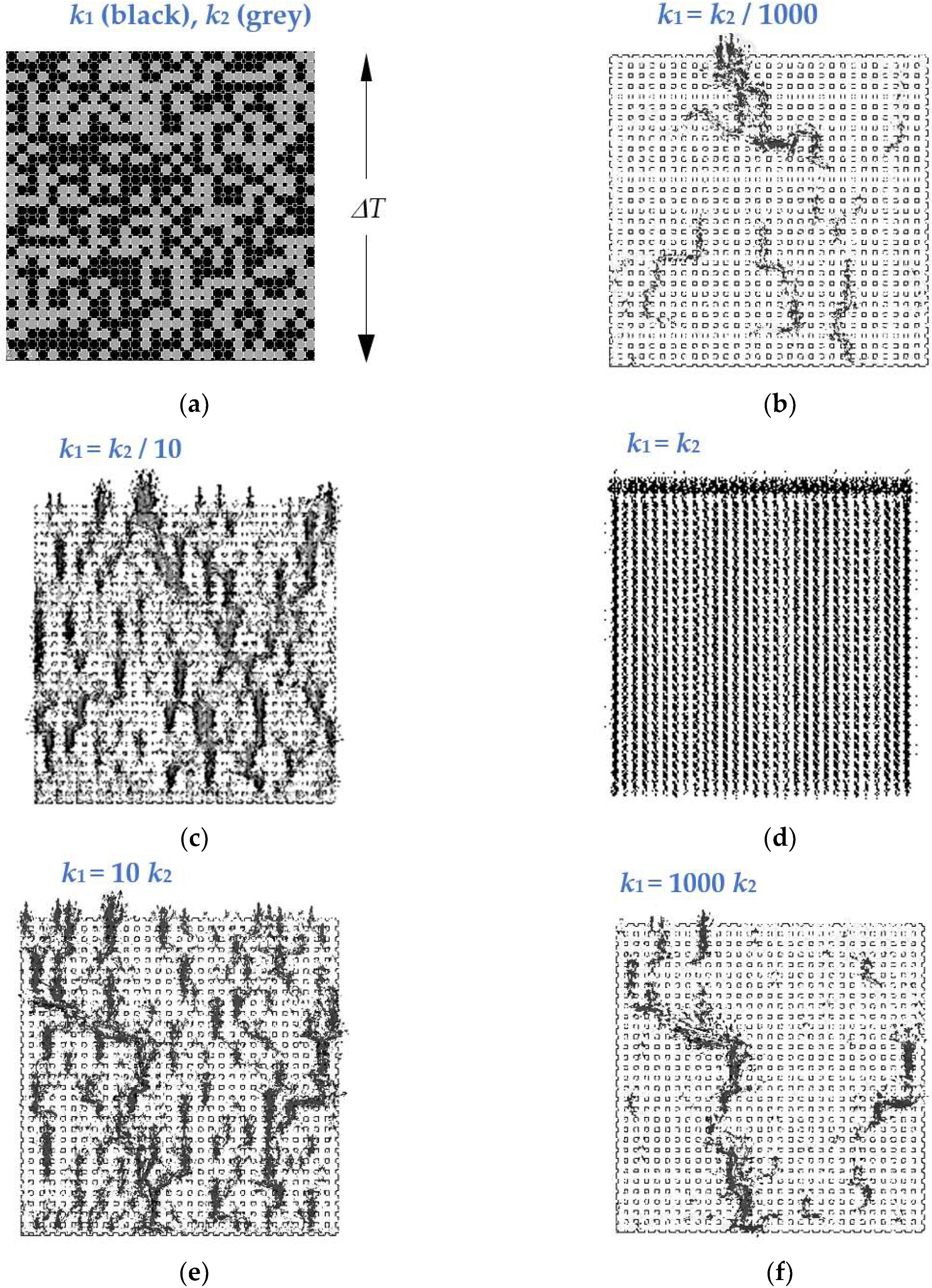
2. Methodology: Construction of Thermal Networks

Figure 1 shows an example of a typical thermal network model used in this work, which was produced by the finite element method (ANSYS, version 8.0, Ansys Inc., Canonsburg, PA, USA). Networks were constructed based on a 30 by 30 array of two different materials of thermal conductivity k₁ (black phase) and k₂ (grey phase), where α₁ is the volume fraction of k₁ and α₂ is the volume fraction of k₂, and α₁ + α₂ = 1. The size of the thermal network is similar to that previously used to study electrical [19] and mechanical [21] networks. A constant temperature of T = 0 °C was applied to the upper region of the network and a constant heat flux was applied to the base of the network, which was constrained to the same temperature; see Figure 1. Heat flow across the corners of particles was avoided by a small region of zero thermal conductivity at the corners of each particle, as can be seen in Figure 1. By considering thermal conduction, with no convection or radiation effects, the temperature difference across the network at equilibrium was determined to estimate the effective thermal conductivity of the network (k_eff).

In the example shown in Figure 1 the volume fraction is α₁ = 0.5. Networks with a range of compositions were examined to explore the influence of the presence of percolation paths of k₁ or k₂ across the network on thermal response. The term percolation is used in this paper to describe the condition where there is a random pathway of one type of material (black or grey in Figure 1) across the network. For α₁ = 0.5, there was an equal probability for percolation of either k₁ or k₂ across the network, while for a fraction of α₁ = 0.7, it was more probable that k₁ was percolated across the network. Likewise, for a network of α₁ = 0.3, it was more probable that k₂ percolated. For each volume fraction examined (α₁ = 0.3, 0.5 and 0.7), twelve different random networks were examined to explore the variation in effective thermal conductivity as a result of the different random arrangements of phases k₁ and k₂. In order to provide a large range of contrasting k₁ and k₂ magnitudes for the thermal networks and explore mixtures containing phases of different thermal conductivity, the thermal contrast (k = k₁/k₂) between the two phases was varied for each network. This spanned the conditions of: (i) k = 10⁻⁴, where heat is likely to flow through the k₂ phase, (ii) k ~ 1, where heat is likely to flow through both phases, and (iii) k = 10⁴, where heat is likely to flow through the k₁ phase. This was achieved by setting k₂ to a constant value of 1 W·m⁻¹·K⁻¹ and varying k₁ from 10⁻⁴ to 10⁴ W·m⁻¹·K⁻¹.

3. Results and Discussion

Thermal networks with randomly distributed elements were modelled with a range of k₁ and k₂ volume fractions (α₁ = 0.3, 0.5 and 0.7) and twelve individual random networks were analysed at each volume fraction, to examine the variability of the network thermal conductivity as a consequence of the different random distributions of the k₁ and k₂ phases within each network.

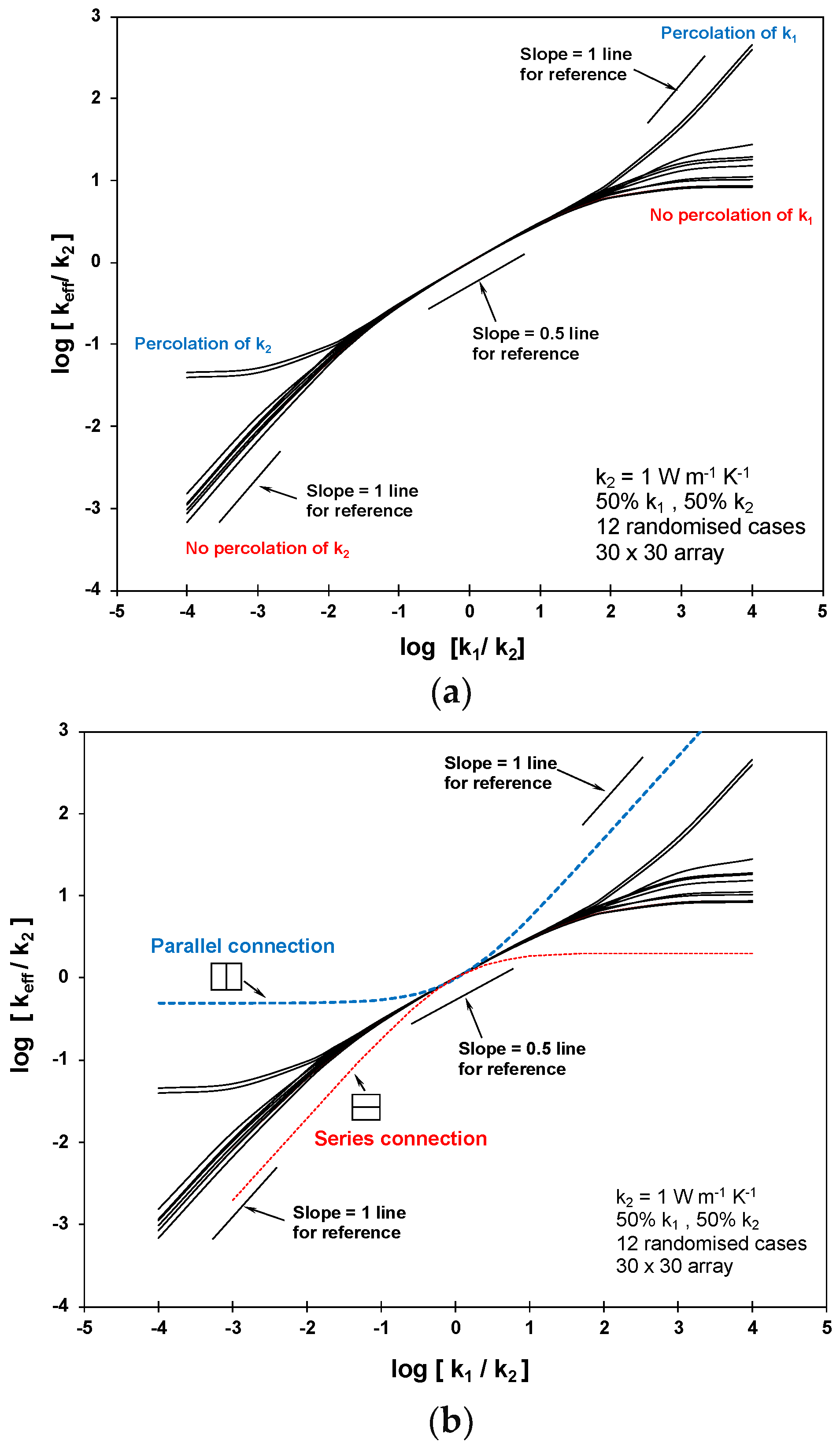
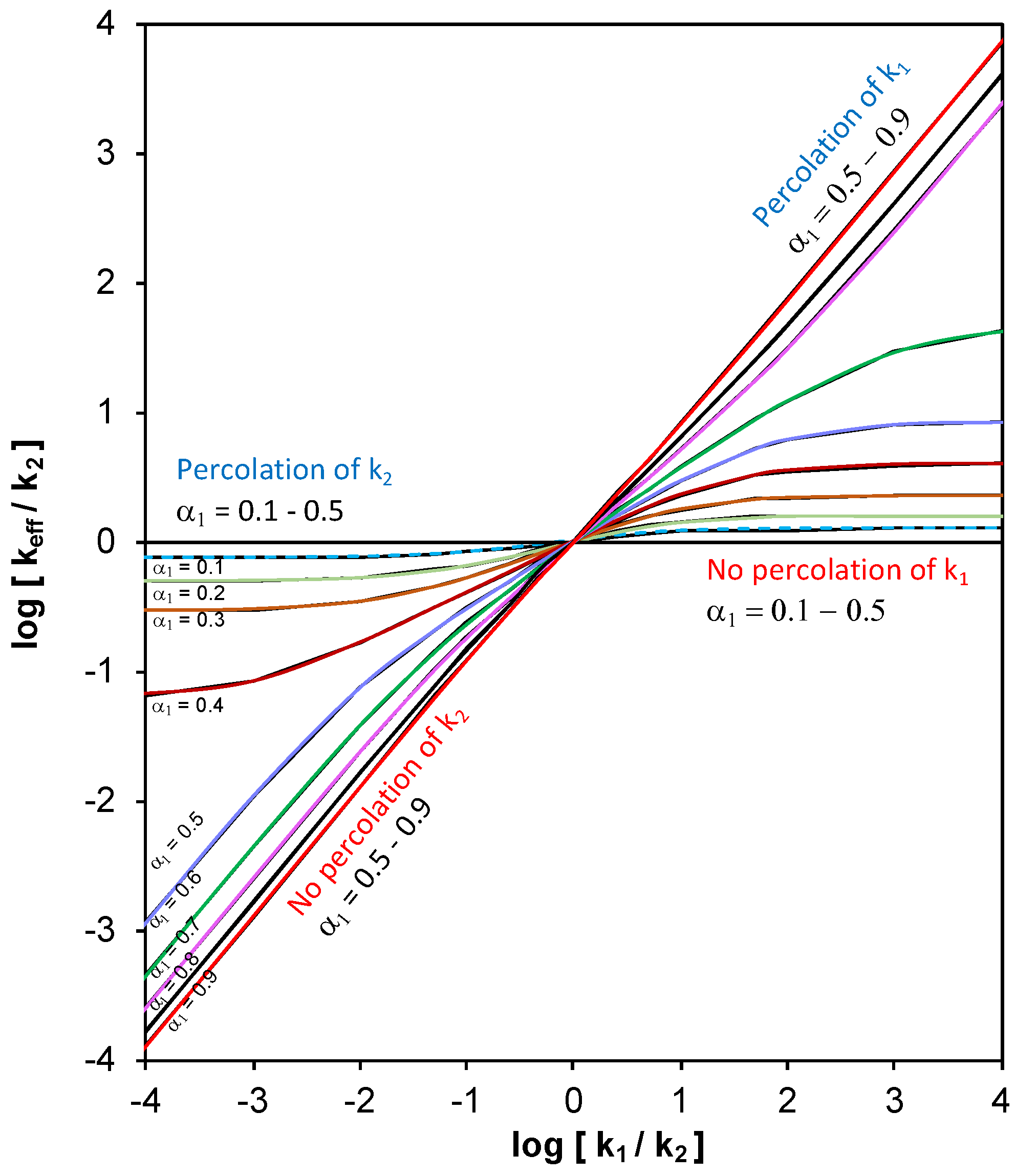
3.1. Thermal Networks with α₁ = 0.5

The thermal network output for twelve realisations of the random network with a 50:50 ratio of k₁:k₂ (namely α₁ = 0.5) are shown in Figure 2. At conditions of high contrast in thermal conductivity of the individual phases (left- or right-hand of Figure 2), the thermal conductivity of each network is sensitive to the distribution of the phases across the network, as it prefers to flow through k₁ or k₂; see Figure 3b,f. However, the thermal networks have an emergent region in the central region of Figure 2, where there is a low variability in the thermal conductivity of individual random networks. In the central region, the contrast (k = k₁/k₂) between the two phases values is relatively low (k₁/k₂ ~ 10⁻² to 10²) and the heat flux can flow through both phases, as seen in Figure 3c–e. As a result, there is a low dependency of effective thermal conductivity on the arrangement of the network.

In the region of low network variance, which we define as the emergent region, a logarithmic mixing rule can be used to describe the effective thermal conductivity (k_eff) of the network,

$$k_{\mathrm{eff}}=k_1^{{\alpha }_1} k_2^{1-{\alpha }_1}$$

(1)

Dividing Equation (1) by k₂ gives rise to,

$$\frac{k_{\mathrm{eff}}}{k_2}={\left[\frac{k_1}{k_2}\right]}^{{\alpha }_1}$$

(2)

From Equation (2), the gradient of log (k_eff/k₂) versus log (k₁/k₂), as shown Figure 2, equals the fraction of material with thermal conductivity k₁ (namely α₁). Figure 2 shows that there is good agreement between the slope of the emergent region in the centre of Figure 2 and the volume fraction of k₁. Similar observations have been made on resistor-capacitor [17,18], capacitor-capacitor [20] and mechanical networks [21], and the log[k₁/k₂] extent of the emergent region has been shown to increase with network size [25,26].

3.2. Origin of the Power-Law

The origin of such a power law has been discussed for dielectric [19,27,28], mechanical [21] and thermal mixtures [17]. For a random array of particles, the random nature of the inter-connections ensures that locally, within the network, it is equally possible to find components that are either connected in series or in parallel. Each case is initially considered, where for a parallel connection,

$$k_{\mathrm{eff}}={\alpha }_1{k}_1+\left(1-{\alpha }_1\right)k_2$$

(3)

At extremes of contrast for a parallel condition, when k₁ << k₂ and k₁/k₂ is small then $k_{\mathrm{eff}}\propto k_2$, leading to a flattening of the blue line in Figure 2b. When k₁ >> k₂ and k₁/k₂ is large, then $k_{\mathrm{eff}}\propto k_1$, leading to a line of gradient of one in Figure 2b. For n parallel components with fraction ${\alpha }_n$ and thermal conductivity $k_n$, this can be generalised to,

$$k_{\mathrm{eff}}={\displaystyle \sum }{\alpha }_n{(k_n)}^1, \mathrm{where} {\displaystyle \sum }{\mathsf{\alpha }}_{\mathrm{n}}=1$$

(4)

For the case of series connection,

$$k_{\mathrm{eff}}^{-1}={\alpha }_1{k}_1^{-1}+\left(1-{\alpha }_1\right)k_2^{-1}$$

(5)

At extremes of contrast for the series case, when k₁ << k₂ and k₁/k₂ is small then $k_{\mathrm{eff}}\propto k_1$, leading to the red line with a gradient of one in Figure 2b. When k₁ >> k₂ and k₁/k₂ is large, then $k_{\mathrm{eff}}\propto k_2$, leading to a flattening of the red line in Figure 2b. For n series components this can be generalised to,

$${\left(k_{\mathrm{eff}}\right)}^{-1}={\displaystyle \sum }{\alpha }_n{\left(k_n\right)}^{-1}$$

(6)

Figure 2b shows that the randomly organised thermal networks exhibit an effective thermal conductivity that is located between the parallel and series bounds; namely between the blue and red lines in Figure 2b, respectively. A generalised case between the upper bound (parallel) and lower bound (series) can therefore be considered as,

$${\left(k_{\mathrm{eff}}\right)}^{\mathrm{v}}={\displaystyle \sum }{\alpha }_{\mathrm{n}}{\left(k_{\mathrm{n}}\right)}^{\mathrm{v}}\hspace{1em}\hspace{1em}\left(-1\le \mathrm{v}\le 1\right)$$

(7)

A random mixture lies between the two cases of the series and parallel bounds, therefore if $\mathrm{v}\to 0$ the approximation of ${\left(\mathrm{x}\right)}^{\mathrm{n}}\to$ 1 + $\mathrm{n}\ln \mathrm{x}$ is valid and Equation (7) becomes,

$$\ln k_{\mathrm{eff}}={\displaystyle \sum }{\alpha }_n\ln k_n$$

(8)

Equation (8) results in the logarithmic mixing law of Equation (1), which can be used to describe the network response when the contrast in thermal conductivity between the two phases is not too large; this corresponds to the condition k₁/k₂ ~ 10⁻² to 10² in Figure 2.

When there is a high contrast in thermal conductivity (high or low k₁/k₂) in the network, the variability between the individual networks of the same composition increases; see the left- or right-hand side of Figure 2. At these high contrast conditions, the inter-connectivity of the two phases is important due to presence, or lack of, percolation paths of inter-connected k₁ or k₂ region. As an example, when k₁ >> k₂ and k₁/k₂ is high, the heat will preferentially flow through k₁. This is clearly evident in Figure 3b,f, where the contrast k = 10⁻³ (heat flows through the grey k₂ regions) and k = 10³ (heat flows through the black k₂ regions), respectively.

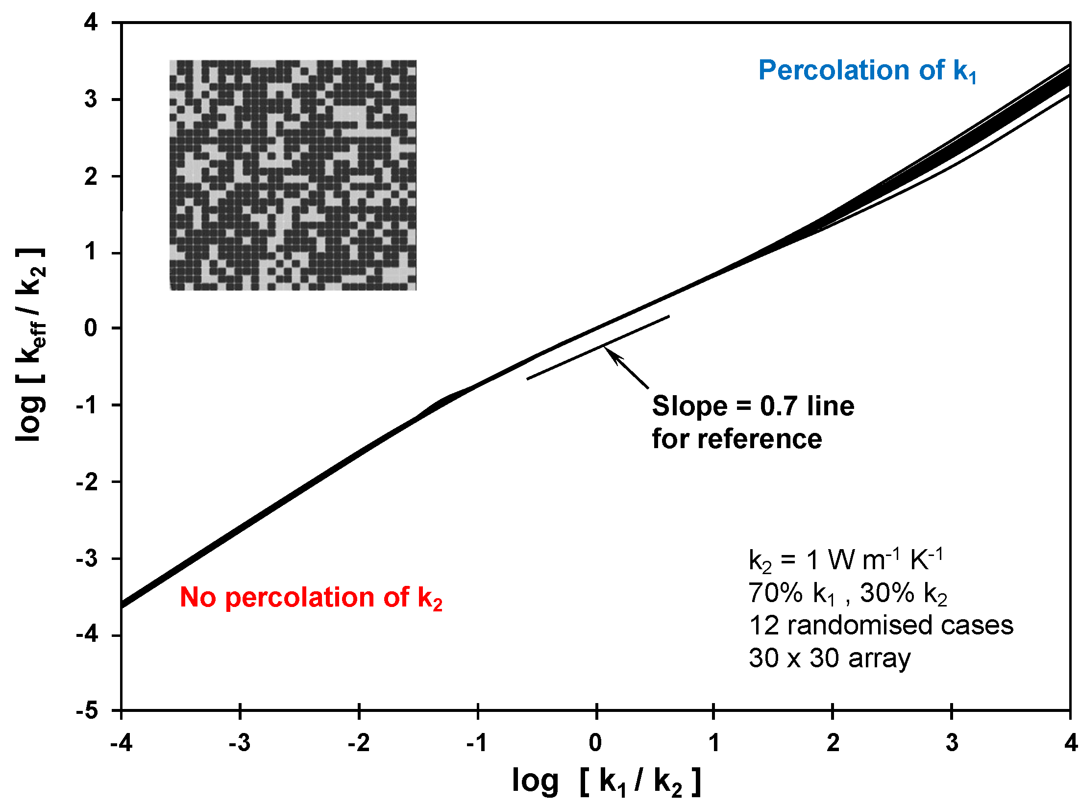
3.3. Thermal Networks with α₁ = 0.7

The thermal network response for a 70:30 ratio of k₁ and k₂ (namely α₁ = 0.7) is shown in Figure 4. As can be seen in the inset image of Figure 4, the k₁ regions (black) are present in greater amounts, and are more likely to percolate across the network, while k₂ (grey) is in the minority and is therefore less likely to percolate across the network. For this type of network, since the k₁ (black) regions are highly interconnected, when k₁ → 0 and k₁ << k₂ (left-hand side of Figure 4), the thermal conductivity approaches zero. When k₁ >> k₂ and k₁ → ∞ the thermal conductivity of the network approaches infinity, corresponding to right-hand side of Figure 4. In the central emergent region, there is again limited variability between the 12 individual networks of the same composition. This also a good correlation between the slope of the network response with the fraction of k₁, with a predicted gradient of 0.7 from Equation (1).

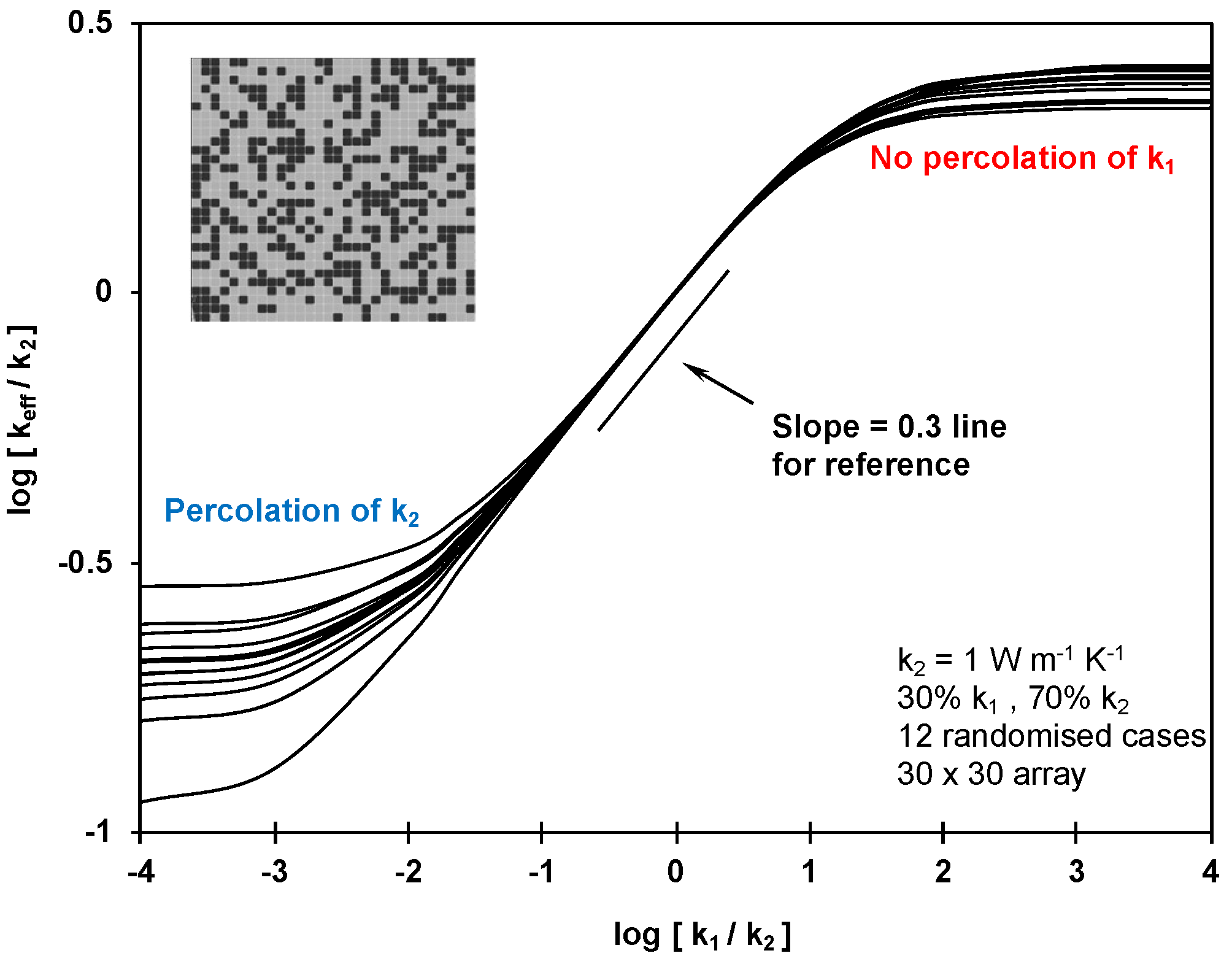
3.4. Thermal Networks with α₁ = 0.3

The response of a network with a 30:70 ratio of k₁ and k₂, namely α₁ = 0.3, is shown in Figure 5. For a 30:70 ratio of k₁:k₂ regions (namely α₁ = 0.3), there is a limited number of k₁ (black) components and they are therefore unlikely to percolate across the network, while there is a majority of k₂ (grey) regions, which are therefore likely to percolate across through the network; see inset of Figure 5 for an example of such a network. In this case, when k₁ << k₂ the k₁ regions act to limit heat flow and the network value approaches a constant value (left-hand side Figure 5), which is dependent on the extent of the percolated region of k₂. The variability observed between individual thermal networks of the same composition is dependent on the level of tortuosity of the k₂ percolation paths for each network. When k₁ >> k₂, the k₁ regions have high thermal conductivity and the network approaches another constant, but larger, value (right-hand side in Figure 5), which is a mixture of k₁ and k₂ phases; again, the variability depends on the fraction of k₁ and k₂ that contribute to the thermally conductive path at this condition. Clearly, in the central emergent region, the response is less network dependent, as heat is able to flow through both k₁ and k₂ regions in a similar manner to Figure 3c–e. There is also good correlation between the slope of Figure 5 and the k₁ fraction of α₁ = 0.3, as predicted by the logarithmic mixing rule of Equation (1).

Figure 6 presents a summary of the typical thermal response of thermal networks for a complete range of compositions, namely α₁ = 0.1–0.9. At the extremes of thermal conductivity contrast where k₁/k₂ < 10⁻² or k₁/k₂ >10², the gradient becomes zero or one, as the heat transfer is dominated by a series or parallel connection of k₁ or k₂ regions. In the central emergent region, the gradient can be seen to gradually increase as the fraction of k₁ increases from 0.1 to 0.9, as is predicted by Equation (1). This form of overall response in Figure 6 is also comparable, qualitatively, with data presented by Ackermann et al. [13] and Hsu et al. [16], although this work has demonstrated that when the contrast in thermal conductivities of the two phases is modest, the thermal networks exhibit an emergent response with a low variability in the effective thermal conductivity of mixtures of the same composition. However, at conditions of high contrast individual networks of the same composition become sensitive to the spatial distribution of the constituents and the presence of series or parallel connected percolation paths across the network, with a gradient of zero or one in Figure 6.

4. Application of Thermal Networks

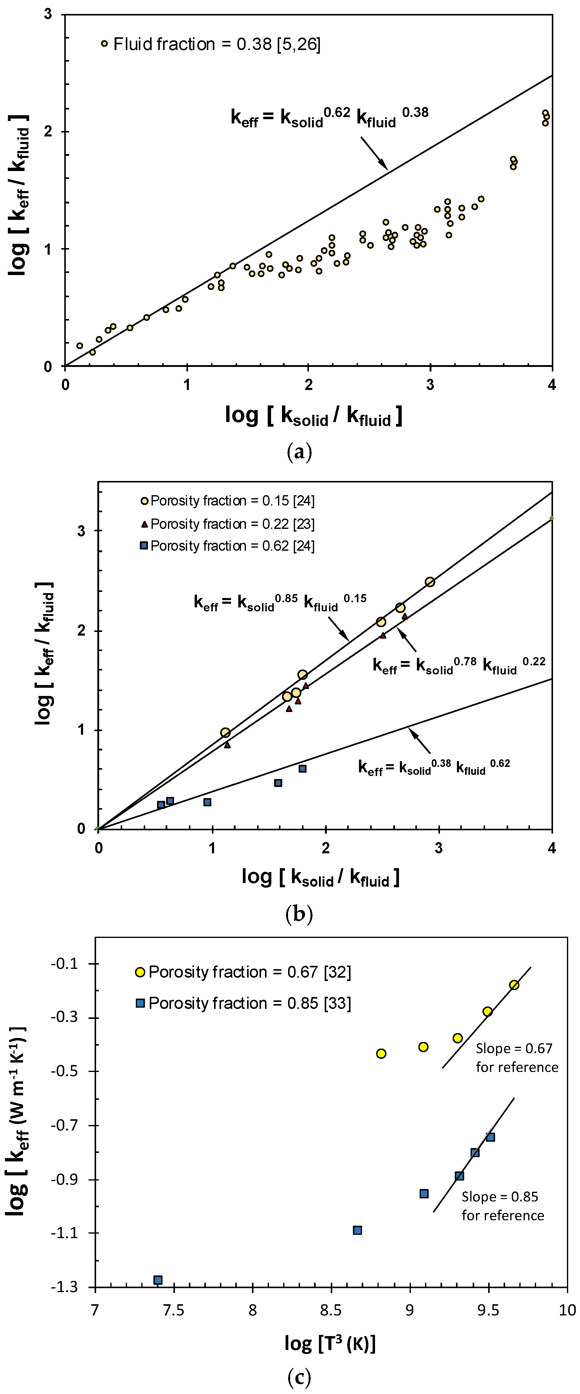
4.1. Comparison with Experimental Data

While good agreement between the logarithmic mixing rule and the thermal networks is observed, it is of interest to compare the mixing rule with experimental data. This would need a mixture of two phases on known volume fraction (α₁ and α₂), where one phase can be changed in value and spans the conditions of low to large contrast, k = k₁/k₂. Such materials and multi-phase systems have been explored, such as packed powder beds, granular media and porous materials filled with different saturants [11,12,29,30,31,32,33,34].

Figure 7a presents data summarised by Kaviany [32], based on the work of Nozad et al. [11,12], for beds of packed particles (with thermal conductivity, k_solid) that are filled with fluids (k_fluid) with a fraction of 0.38. Good correlation is observed with the power law mixing rule, Equation (1), for low thermal contrast (k_solid/k_fluid ≲ 10^1.5), but the agreement is lost at higher levels of contrast, as is observed in the thermal network models. Figure 7b present data presented by Woodside et al. [29] and summarised by Feng et al. [30], which include porous rocks filled with different media; in this case good agreement with the power law is observed for conditions up to k_solid/k_fluid ≲ 10³. The good agreement with experimental data indicates that the mixing rule can be used for prediction of the effective conductivity of multi-phase mixtures at moderate levels of thermal conductivity contrast.

4.2. Thermal Conduction in Porous Materials

Another example of thermal networks which experience a range of thermal conductivity contrast values between their individual phases is porous refractories and ceramics at elevated temperatures. These materials are of interest as high temperature insulation materials for space, aerospace, power generation and high temperature processing applications [35,36,37]. It is assumed that the material contains pores at a porosity fraction, p, and represents a two-phase system, consisting of a refractory ceramic, which can be assumed to have a relatively temperature insensitive thermal conductivity (k_ceramic) and pores, of which the thermal conductivity (k_pore) is sensitive to temperature, due to radiation heat transfer across pore surfaces. At low temperatures, the thermal conductivity of the pore is small, and the effective conductivity is dominated by the ceramic (k_ceramic >> k_pore). At a sufficiently high temperature, radiation across pores increases so that the condition (k_ceramic ~ k_pore) is met and the effective conductivity of the porous material can be described by the logarithmic mixing rule, namely

$$k_{\mathrm{eff}}=k_{\mathrm{pore}}^p k_{\mathrm{ceramic}}^{1-p}$$

(9)

The effective thermal conductivity of a pore due to thermal radiation has a strong temperature dependence and can be estimated from:

$$k_{\mathrm{pore}}=4ϵ\sigma \gamma d_p{T}^3$$

(10)

where $ϵ$ is the emissivity, $\sigma$ is the Stefan–Boltzmann constant, $\gamma$ is a geometric factor ($0\le \gamma \le 1)$ that depends on pore shape, $d_p$ is the maximum width of the pore with respect to the thermal gradient and T is the absolute temperature. Substitution of Equation (10) into Equation (9) gives rise to,

$$k_{\mathrm{eff}}={\left(4ϵ\sigma \gamma d_p\right)}^p k_{\mathrm{ceramic}}^{1-p}{\left(T^3\right)}^p$$

(11)

This leads to a power-law temperature dependency of the effective thermal conductivity,

$$\frac{k_{\mathrm{eff}}}{k_{\mathrm{ceramic}}^{1-p}} \propto {\left(T^3\right)}^p$$

(12)

If the thermal conductivity of the ceramic is relatively insensitive to temperature in the temperature range of interest then,

$$k_{\mathrm{eff}}\propto {\left(T^3\right)}^p$$

(13)

Therefore, in the emergent region where k_ceramic ~ k_pore, the thermal conductivity of the porous materials should be proportional to T^3p and a graph of log(k_eff) against log(T³) should have a gradient that is equal to the porosity fraction of the material at high temperature. Figure 7c presents experimental high temperature thermal conductivity measurements on refractory ceramics [38] and aerogels/fibrous ceramic composites [39] at temperatures up to 1600 K. Relatively good correlation between the slope and the fraction of porosity based on Equation (13) can be observed. Potential errors can be the assumption of not taking into account the change in k_ceramic in the temperature range (which can be reduced using Equation (12), if the data is known) and other contributions to effective conductivity, such as convection within pores or changes in the conductivity of the gas within pores with temperature. In this case, the application of thermal networks provides a new method to interpret and predict the high temperature conductivity of porous ceramics and refractories.

5. Conclusions

This paper has examined the properties of thermal networks to understand the effective thermal conductivity of two-phase composite materials and systems. At conditions of high contrast in thermal conductivity of the two phases, namely when k₁ << k₂ or k₁ >> k₂, the effective thermal conductivity of thermal networks at the same composition exhibited greater variability and were sensitive to the connectivity of the phases and presence of percolation paths across the network. However, when the contrast in thermal conductivities of the two phases are more modest (k₁/k₂ ~ 10⁻² to 10²) the thermal networks exhibit an emergent region where there is a low variability in the effective thermal conductivity of random mixtures of the same composition. It has been shown that for the two-phase thermally conductive composites, a logarithmic mixing rule can be used to predict the effective conductivity in the emergent region, thereby providing a rapid and simple approach to predicting the thermal properties. This region is also of interest in the design of new composites with predictable and isotropic properties, since in this region both phases are contributing to the effective conductivity, thereby inherently leading to reduced variability. The work provides new limits for the use of such mixing rules for multi-phase systems, since at conditions of high contrast in thermal conductivity, the heat flow is strongly governed by the percolation paths across the network and no longer follows the logarithmic mixing rule and is dominated by series or parallel connected percolation paths.

Good agreement with experimental data was observed for a range of multi-phase media such as packed beds and porous media filled with a range of fluids. The potential of the approach to provide new methods to interpret the temperature dependent behaviour of high temperature ceramics was demonstrated. This new approach can inform future directions on multi-phase systems; these can include the extension of the concept to three-dimensional systems, where the percolation paths can be three-dimensional in nature, an extension to thermal mixtures with more than two phases, and the introduction of interfacial resistances or thermal stresses. The modelling approach therefore provides new insights for the design of heterogeneous multi-phase composites for thermal management applications and the interpretation and prediction of their thermal response.

References

1. Guerra, V.; Wan, C.; McNally, T. Thermal conductivity of 2D nano-structured boron nitride (BN) and its composites with polymers. Prog. Mater. Sci. 2019, 100, 170–186. [Google Scholar] [CrossRef]
2. Kosbe, P.; Patil, P. Effective thermal conductivity of polymer composites: A review of analytical methods. Int. J. Ambient Energy 2019, 1–12. [Google Scholar] [CrossRef]
3. Fraleoni-Morgera, A.; Manisha Chhikara, M. Polymer-based nano-composite for thermal insulation. Adv. Eng. Mater. 2019, 21, 1801162. [Google Scholar] [CrossRef]
4. Huang, Y.; Ellingford, C.; Bowen, C.; McNally, T.; Wu, D.; Wan, C. Tailoring the electrical and thermal conductivity of multi-component and multi-phase polymer composites. Int. Mater. Rev. 2020, 65, 129–163. [Google Scholar] [CrossRef]
5. Xue, Y.; Lofland, S.; Hu, X. Thermal conductivity of protein-based materials: A review. Polymers 2019, 11, 456. [Google Scholar] [CrossRef] [Green Version]
6. Zhan, H.; Nie, Y.; Chen, Y.; Bell, J.M.; Gu, Y. Thermal transport in 3D nanostructures. Adv. Funct. Mater. 2020, 30, 1903841. [Google Scholar] [CrossRef] [Green Version]
7. Chen, H.; Ginzburg, V.V.; Yang, J.; Yang, Y.; Liu, W.; Huang, Y.; Du, L.; Chen, B. Thermal conductivity of polymer-based composites: Fundamentals and applications. Prog. Polym. Sci. 2016, 59, 41–85. [Google Scholar] [CrossRef]
8. Burger, N.; Laachachi, A.; Ferriol, M.; Lutz, M.; Toniazzo, V.; Ruch, D. Review of thermal conductivity in composites: Mechanisms, parameters and theory. Prog. Polym. Sci. 2016, 61, 1–28. [Google Scholar] [CrossRef]
9. Huang, C.; Qian, X.; Yang, R. Thermal conductivity of polymers and polymer nanocomposites. Mater. Sci. Eng. Rep. 2018, 132, 1–22. [Google Scholar] [CrossRef] [Green Version]
10. Xu, J.; Gao, B.; Du, H.; Kang, F. A statistical model for effective thermal conductivity of composite materials. Int. J. Therm. Sci. 2016, 104, 348–356. [Google Scholar] [CrossRef]
11. Nozad, I.; Carbonell, R.G.; Whitaker, S. Heat conduction in multi-phase systems I: Theory and experiments for two-phase systems. Chem. Eng. Sci. 1985, 40, 843–855. [Google Scholar] [CrossRef]
12. Nozad, I.; Carbonell, R.G.; Whitaker, S. Heat conduction in multi-phase systems II: Experimental method and results for three-phase systems. Chem. Eng. Sci. 1985, 40, 857–863. [Google Scholar] [CrossRef]
13. Ackermann, S.; Scheffe, J.R.; Duss, J.; Steinfeld, A. Morphological characterization and effective thermal conductivity of dual-scale reticulated porous structures. Materials 2014, 7, 7173–7195. [Google Scholar] [CrossRef] [PubMed] [Green Version]
14. Jia, G.S.; Tao, Z.Y.; Meng, X.Z.; Ma, C.F.; Chai, J.C.; Jin, L.W. Review of effective thermal conductivity models of rock-soil for geothermal energy applications. Geothermics 2019, 77, 1–11. [Google Scholar] [CrossRef]
15. Deissler, R.G.; Boegli, J.S. An investigation of effective thermal conductivities of powders in various gases. ASME Trans. 1958, 80, 1417–1425. [Google Scholar]
16. Hsu, C.T.; Cheng, P.; Wong, K.W. A lumped parameter model for stagnant thermal conductivity of spacially periodic porous media. J. Heat Transf. 1995, 117, 264–269. [Google Scholar] [CrossRef]
17. Agari, Y.; Uno, T. Estimation on thermal conductivities of filled polymers. J. Appl. Polym. Sci. 1986, 32, 5705–5712. [Google Scholar] [CrossRef]
18. Vainas, B.; Almond, D.P.; Luo, L.; Stevens, R. An evaluation of random RC networks for modelling the bulk ac electrical response of ionic conductors. Solid State Ion. 1999, 126, 65–80. [Google Scholar] [CrossRef]
19. Almond, D.P.; Vainas, B. The dielectric properties of random R–C networks as an explanation of the ‘universal’ power law dielectric response of solids. J. Phys. Cond. Matter 1999, 11, 9081–9093. [Google Scholar] [CrossRef]
20. Richardson, P.; Almond, D.P.; Bowen, C.R. A study of random capacitor networks to assess the emergent properties of dielectric composites. Ferroelectrics 2009, 391, 158–167. [Google Scholar] [CrossRef]
21. Murphy, K.D.; Hunt, G.W.; Almond, D.P. Evidence of emergent scaling in mechanical systems. Philos. Mag. 2006, 86, 3325–3338. [Google Scholar] [CrossRef]
22. Maxwell, J.C. A Treatise on Electricity and Magnetism; Clarendon Press: Oxford, UK, 1881. [Google Scholar]
23. Lichtenecker, K. Die dielektrizitätskonstante natürlicher und Künstlicher Mischkörper. Phys. Z. 1926, 27, 115–158. [Google Scholar]
24. Lichtenecker, K.; Rother, K. Die Herleitung des logarithmischen Mischungs-gesetzes aus allegemeinen Prinzipien der stationaren Stromung. Phys. Z. 1931, 32, 255–260. [Google Scholar]
25. Almond, D.P.; CJ Budd, C.J.; Freitag, M.A.; Hunt, G.W.; McCullen, N.J.; Smith, N.D. The origin of power-law emergent scaling in large binary networks. Phys. A Stat. Mech. Appl. 2013, 392, 1004–1027. [Google Scholar] [CrossRef] [Green Version]
26. Aouaichia, M.; McCullen, N.; Bowen, C.R.; Almond, D.P.; Budd, C.; Bouamrane, R. Understanding the anomalous frequency responses of composite materials using very large random resistor-capacitor networks. Eur. Phys. J. B 2017, 90, 39. [Google Scholar] [CrossRef] [Green Version]
27. Truong, V.T.; Ternan, J.G. Complex conductivity of a conducting polymer composite at microwave frequencies. Polymer 1995, 36, 905–909. [Google Scholar] [CrossRef]
28. Moulson, A.J.; Herbert, J.M. Electroceramics, 2nd ed.; John Wiley & Sons: Chichester, UK, 2003; pp. 82–85. [Google Scholar]
29. Woodside, W.; Messmer, J.H. Thermal conductivity of porous media. II. Consolidated rocks. J. Appl. Phys. 1961, 32, 1699–1706. [Google Scholar] [CrossRef]
30. Feng, Y.; Yu, B.; Zou, M.; Zhang, D. A generalized model for the effective thermal conductivity of porous media based on self- similarity. J. Phys. D Appl. Phys. 2004, 37, 3030–3040. [Google Scholar] [CrossRef]
31. Shonnard, D.R.; Whitaker, S. The effective thermal conductivity for a point- contact porous medium: An experimental study. J. Heat Mass Transf. 1989, 32, 503–512. [Google Scholar] [CrossRef]
32. Kaviany, M. Conduction heat transfer. In Principles of Heat Transfer in Porous Media; Mechanical Engineering Series; Springer: New York, NY, USA, 1995; pp. 119–156. [Google Scholar]
33. Kandula, M. On the effective thermal conductivity of porous packed beds with uniform spherical particles. J. Porous Media 2011, 14, 919–926. [Google Scholar] [CrossRef] [Green Version]
34. Takatsu, Y.; Masuoka, T.; Nomura, T.; Yamada, Y. Modeling of effective stagnant thermal conductivity of porous media. J. Heat Mass Transf. 2016, 138, 12601. [Google Scholar] [CrossRef]
35. Tychanicz-Kwiecien, M.; Wilk, J.; Gil, P. Review of high-temperature thermal insulation materials. J. Thermophys. Heat Transf. 2018, 33, 271–284. [Google Scholar] [CrossRef]
36. Bakker, K.; Kwast, H.; Cordfunke, E.H.P. The contribution of thermal radiation to the thermal conductivity to porous UO2. J. Nucl. Mater. 1995, 223, 135–142. [Google Scholar] [CrossRef]
37. Loeb, A.L. Thermal conductivity: VIII, A theory of thermal conductivity of porous materials. J. Am. Ceram. Soc. 1954, 37, 96–99. [Google Scholar] [CrossRef]
38. He, L.; Zhang, M.; Gu, H.; Huang, A. The influence of thermal radiation on effective thermal conductivity in porous material. Interceram 2016, 65, 237–243. [Google Scholar] [CrossRef]
39. He, J.; Li, X.; Su, D.; Ji, H.; Wang, X. Ultra-low thermal conductivity and high strength of aerogel/fibrous ceramic composites. J. Eur. Ceram. Soc. 2016, 36, 1487–1493. [Google Scholar] [CrossRef]
Figure 1. An image of a typical 30 × 30 thermal network, where α1 = 0.5. A heat flux was applied to the base, all of which are to the same temperature. The upper section of the network was held at 0 °C. Phase k1 (black) has a variable thermal conductivity from 10−4 to 104 W·m−1·K−1 and k2 (grey) is a constant conductivity of 1 W·m−1·K−1.
Jcs 04 00032 g001
Figure 2. (a) Log-log plot of effective conductivity as a function of k1/k2 for 12 different randomizations, each corresponding to a 30 × 30 system, where α1 = 0.5. (b) Series and parallel bounds.
Jcs 04 00032 g002
Figure 3. Heat flux for network for a variety of k1/k2 ratios. (a) Original network, k1 (variable, black), k2 =1 W m−1 K−1 (constant, grey), (b) k1 = k2 /1000, (c) k1 = k2 /10, (d) k1 = k2, (e) k1 = 10 k2, (f) k1 = 1000 k2.
Jcs 04 00032 g003
Figure 4. Log-log plot of the equivalent conductivity as a function of k1/k2 for the 70% k1–30% k2 system (α1 = 0.7). Phase k1 (black) is variable and k2 (grey) is constant.
Jcs 04 00032 g004
Figure 5. Log-log plot of the equivalent conductivity as a function of k1/k2 for the 30% k1–70% k2 system (α1 = 0.3). Phase k1 (black) is variable and k2 (grey) is constant.
Jcs 04 00032 g005
Figure 6. Summary of typical thermal network responses for range of fractions of k11 = 0.1–0.9).
Jcs 04 00032 g006
Figure 7. Comparison of logarithmic mixing rule with experimental data of (a) packed beds [5,26] (b) rocks [29,30] and (c) high temperature porous ceramics [38,39].
Jcs 04 00032 g007