Adaptive Control for Multi-Shaft with Web Materials Linkage Systems

Abstract

In this paper, a fuzzy disturbance observer and a high-gain disturbance observer based on a variable structure controller are applied to deal with imprecise multi-shaft with web materials linkage systems taking into account the variation of the moment of inertia. Specifically, a high-gain disturbance observer and an adaptive fuzzy algorithm are separately applied to estimate system uncertainties and external disturbances. The high-gain disturbance observer is designed with auxiliary variables to avoid the amplification of the measurement disturbance, and the fuzzy disturbance observer has the advantage that it does not depend on model information. The convergence properties of the tracking error are analytically proven using Lyapunov’s theory. The obtained numerical results demonstrate the validity and the adaptive performance of the proposed control law in case the system is exposed to uncertainties and disturbances. Important remarks on the design process and performance benchmarks of the two observers are also demonstrated.

1. Introduction

Multi-shaft with web materials linkage systems are intensively employed in industry [1,2], especially in various applications such as flexible displays, color-shifting, lighting, and solar cell production. Therefore, web tension and velocity controls play an important role in improving the quality of products in processes using web handling technology.

A roll-to-roll system is one of the complex drives and strong nonlinear systems affected by different types of noises, especially when the system is operating at high speed [3]. In order to control the system, the most important task is formulating an accurate mathematical model for the system. In [4], a web transport system with four segments is presented. This model has the advantage that web tension can be calculated for the controller, but it is necessary to have precise measuring devices, and the calculation of the tension to be returned to the controller requires the use of algebraic equations. Studies [5,6] have provided a dynamic model for the multi-roll system; the tension equation has been generalized to the material segments and takes into account the variable length of the material. However, considering the dynamic of rolls, the studies ignore the variation in the radius of the rolls. A recent publication on modeling for a single-span roll-to-roll system, where the tension is determined using a load cell, is presented in [7]. The mathematical model has a nonlinear form with the coefficients specifying the model parameters. This helps the authors to design a nonlinear controller for the system. However, when considering the technological characteristics of the web transport system, the above model does not generalize the steps performed, does not verify the long velocity of the web, and ignores the model’s moment of inertia variation. In the paper, we propose a multi-shaft with web materials linkage model which considers the moment of inertia variation along with the squared component of the velocity and has a suitable form for technological requirements in the case that the variable outputs are the tension and the velocity.

The key point to guarantee the system output quality is to properly handle the velocity and tension of webs. In particular, tension control is considered as a key factor in controlling roll-to-roll systems because low tension leads to wrinkles in the web, and a non-compact rewinding system and over-tension causes web breakage, resulting in serious production efficiency and financial problems. The solution to the web control problem considered in [8,9] using classical proportional integral derivative (PID) is easily installed in the industry. However, traditional PID controllers are designed for objects with mathematical models with constant parameter assumptions, leading to the undesired response of the controller to the uncertainty and variations of parameters in the model. In [10], an indirect adaptive proportional integral (PI) control scheme is applied to improve the system performance. In particular, the estimated parameters can be automatically initialized based on the relay feedback technique. Controllers designed by using the backstepping technique have been recently studied, and [11,12,13] have shown for the roll-to-roll system that the quality and stability of the system are guaranteed and the tension over-shoot is small. In fact, the web transport system is affected by various nonlinear elements such as friction, torque, and hardware features, and thus the control quality of the system is reduced, which leads to the phenomenon of the “explosion of terms”. Besides this, sliding mode control is well known in applications such as uncertain nonlinear systems, multiple-input and multiple-output systems, nonlinear systems, continuous systems, complex systems, systems with infinite dimensionality times, etc. Particularly, the studies given in [14,15] indicate that the robust control method with sliding mode control has the advantages of being stable to disturbance factors and less sensitive to the variation of model parameters, especially fast dynamic responses. These studies indicate that dealing with the chattering effect is still of interest because this effect of the controllers especially affects the implementation of digital techniques for real devices. Therefore, we designed sliding mode control for a single-span roll-to-roll system by replacing the saturation function with the sign function in order to eliminate the chattering effect. However, this change leads to a steady-state error remaining in the system, and in order to enhance the tracking performance, some adaptive strategies should be used for disturbance compensation.

In addition, a necessary problem that is relevant while controlling single-span roll-to-roll nonlinear systems is the handling of system disturbances. The reason is that it is extremely difficult to measure the disturbance in most cases due to limitations of space and/or cost concerns. In [16,17], the authors propose an active disturbances rejection controller (ADRC) with an extended state observer which is responsible for monitoring and estimating disturbance. Thanks to advantages such as the ease of adjustment, fast response, and robustness with variable parameters, disturbance-removing controllers are an interesting way to replace traditional PID controllers. In [18], the author proposes a control design based on dynamic surface control as an alternative approach to model-based controllers. The paper also introduces comprehensive numerical simulations to demonstrate the effectiveness of the control design in comparison with the backstepping technique. The dynamic surface control-based controller provides high tracking performance, which is superior to that of the backstepping controller even when the system is adversely affected by the uncertainties. In traditional nonlinear controllers, the high-gain disturbance observer has attracted a great deal of attention due to its simple structure in application. The nonlinear observer has been applied to many systems such as a multi-rotor unmanned aerial vehicle (UAV) in [19], electro-hydraulic systems in [20], a permanent magnet synchronous motor in [21,22,23], et al., giving improved responses when disturbances arise. Besides, disturbance estimation using fuzzy logic is also interesting due to the possibility of expressing human experience in an algorithmic manner. An adaptive controller can be used for imprecise single-input–single output (SISO) nonlinear systems, where fuzzy logic is applied to estimate disturbances for sliding mode control [24]. The problem of disturbance-observer-based adaptive fuzzy control is studied for nonlinear systems with full state constraints, input constraints, and unknown external disturbance in [25]. In [26], an adaptive backstepping sliding mode control method based on a fuzzy disturbance observer is proposed to solve the problem of trajectory tracking control for the manipulator—a kind of nonlinear system with multiple inputs and multiple outputs. In [27], using a descriptor fuzzy model-based framework, the author proposes a new approach to design a feedback–feedforward control scheme for robot manipulators in a general form and shows that the tracking performance is improved when an external disturbance arises. An adaptive controller using radial basis function (RBF) neural network-based backstepping–sliding mode control which could eliminate the existence of nonlinear elements as well as increase the system’s robustness is proposed in [28]. In addition, the problems stemming from backstepping and SMC are also solved, including the “explosion of terms” and chattering. To solve the disturbance occurring in a single-span roll-to-roll nonlinear system, we propose two variable structure controllers, respectively, based on a high-gain disturbance observer and an adaptive fuzzy algorithm.

The novel contributions of the paper can be summarized as follows. (i) In this study, we have successfully built a single-span roll-to-roll nonlinear system with output tension and velocity, taking into account the variation of the moment of inertia along with the squared component of the velocity. (ii) A proposed control structure consisting of a high-gain disturbance observer and adaptive fuzzy algorithm based on sliding mode control is applied in order to estimate uncertain parameters and disturbances which can be measured inaccurately or unknown. Particularly, the amplification of the measurement disturbances is eliminated through introducing auxiliary state variables to the high-gain disturbance observer, and the use of the fuzzy disturbance observer has the outstanding characteristic of reducing dependence on the model while designing disturbance observers but still guarantees the system’s stability and simultaneously copes with uncertainties. (iii) The simulation results verify the performance of the controllers and show the superior response of the two proposed controllers compared to the sliding mode control using the saturation function.

The paper is organized into six parts as follows. The model of the multi-shaft with web materials linkage system is presented in Section 2. Section 3 is dedicated to the design of a sliding mode control for the system. In Section 4, we present an adaptive fuzzy algorithm and a high-gain disturbance observer to cope with imprecise nonlinear systems. The simulation results are given in Section 5. Finally, some concluding remarks are stated in Section 6.

2. Roll-to-Roll Nonlinear System Model

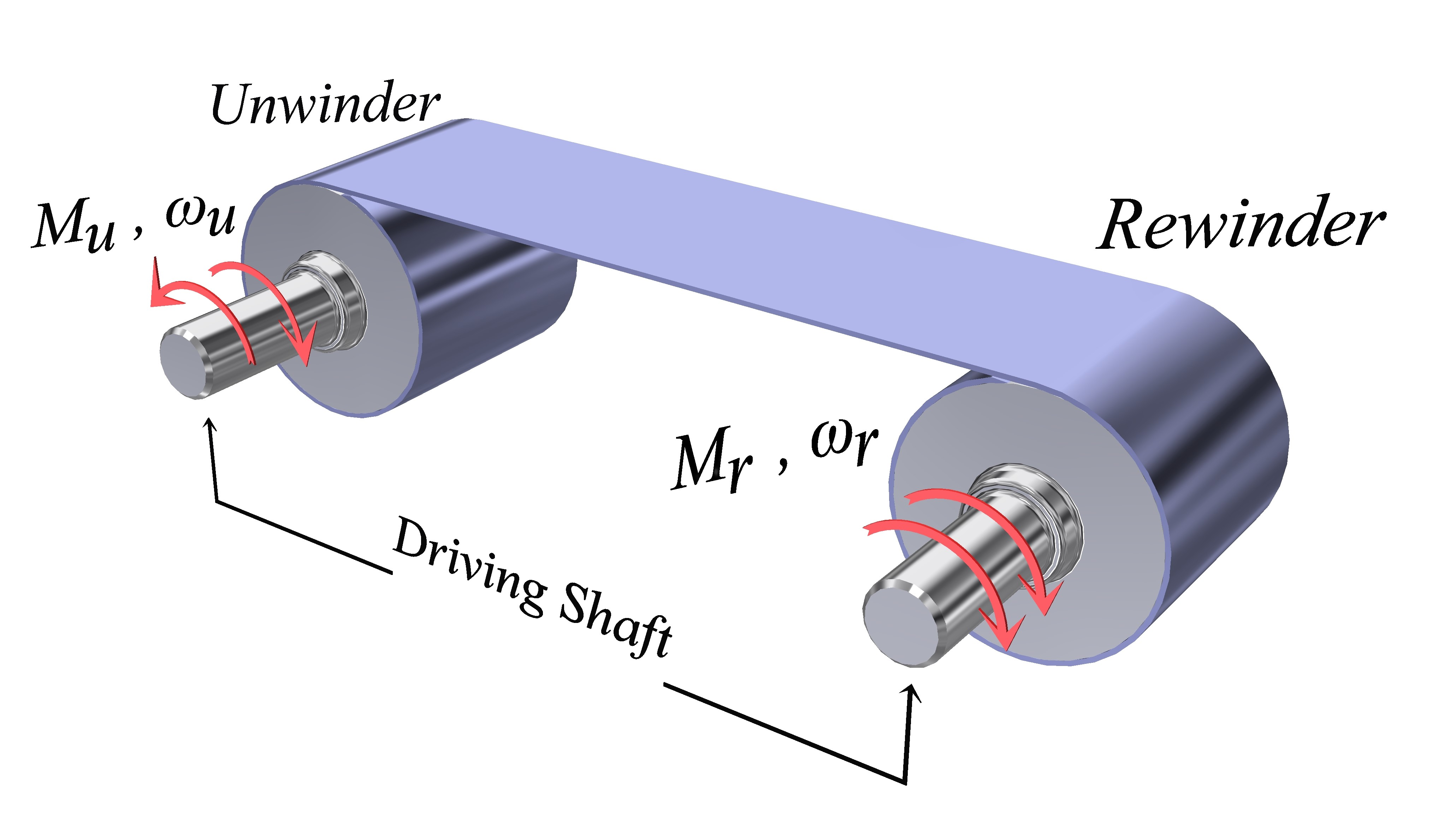
The single-span roll-to-roll nonlinear system has the main components of an unwinder and a rewinder, which are connected through a web of a certain length as shown in Figure 1. In the figure, $M_u$ and $M_r$ are the driving torques on the unwinder and rewinder shaft, and ${\omega }_u$ and ${\omega }_r$ denote the angular velocity of the unwinder and rewinder, respectively.

The mathematical model of the rewinding system is built based on a general model of tension and velocity between two consecutive rolls.

2.1. Web Dynamic

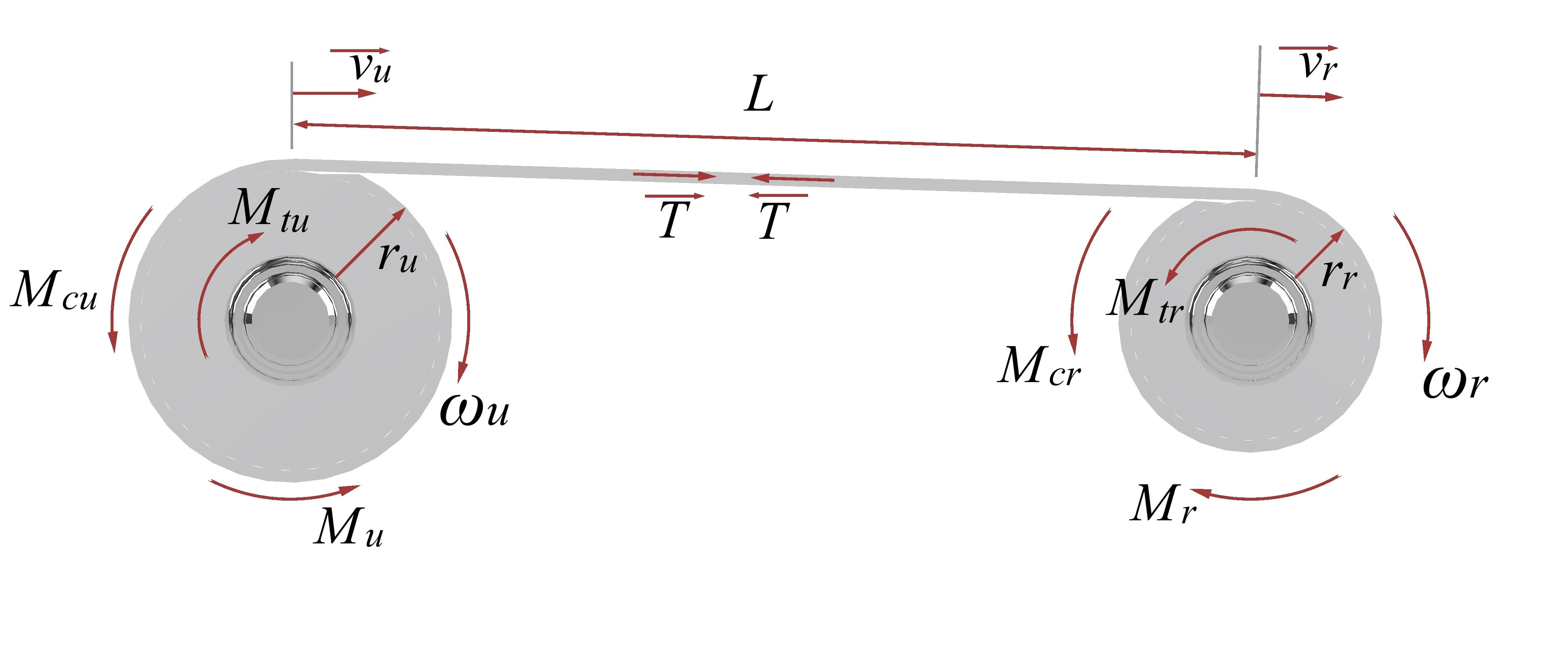
To determine the tension equation of the segment of the web between the unwinder and rewinder, we consider a specific case of the sheet of material between two rolls as shown in Figure 2. In the figure, $M_{tu}$ and $M_{tr}$ denote the torques of the tension force acting on the unwinder and rewinder; $M_{cu}$ and $M_{cr}$ represent the torque due to the frictional force acting on the unwinder and rewinder shaft; $r_u$ and $r_r$ are the operating radii of the unwinder and rewinder; $v_u$ and $v_r$ are the velocity of the unwinder and rewinder; and T and L denote the tension and the total length of the web, respectively.

According to [4], the tension of the rewinding system model is calculated based on three main laws of physics: the Law of Conservation of Mass, Hooke’s Law, and Coulomb’s Law. Thus, we obtain

$$\begin{array}{c}\hfill \frac{LdT}{dt}=ES\left(v_r-v_u\right)+v_u{T}_d-v_{r}T\end{array}$$

(1)

where E denotes the Young’s modulus of the web, S is the cross-sectional area of web, and $T_d$ is the tension on the unwinder.

2.2. Dynamics of Rolls

2.2.1. Unwinder

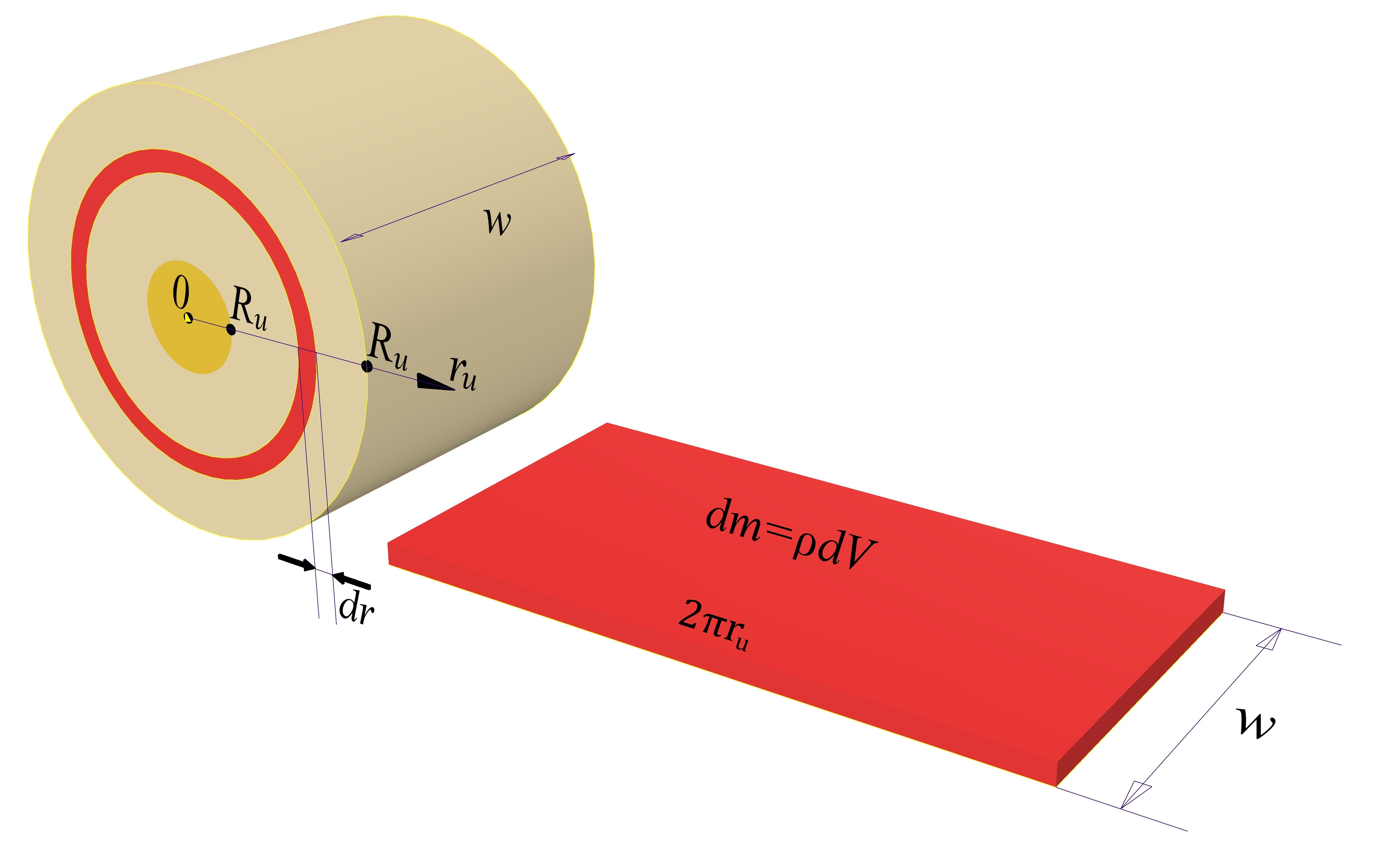
Considering the mass element as in Figure 3, where the thickness of each material layer is $a=dr$, the unwinder width is w, and the density of the web is $\rho$, we obtain

$$\begin{array}{c}\hfill dm=\rho dV=\rho \pi rdrw\end{array}$$

(2)

At the initial time when the unwinder has not unwinded the material, $r_u\left(0\right)=R_u$, where $r_u$ is a radius function with respect to time. Accordingly, the initial moment of inertia $J_u\left(0\right)$ can be calculated as

$$\begin{array}{c}\hfill J_u=J_{u0}+\frac{1}{2}\rho w\pi (r_u^4-R_c^4)\end{array}$$

(3)

$$\begin{array}{c}\hfill {\dot{J}}_u=2\pi w\rho r_u^3{\dot{r}}_u\end{array}$$

(4)

where $J_u$ is the total moment of inertia of the unwind roll, and $R_c$ denotes the radius of the unwinder shaft.

Considering the condition that the material layer thickness a is very small, implying that the radius of the unwinder changes slowly, the rotation angle (rad) of the unwinder can be approximated as:

$$\begin{array}{c}\hfill {\dot{r}}_u=-a\frac{v_u}{2\pi r_u}\end{array}$$

(5)

The angular momentum variation for the unwinder is depicted in Figure 2. Projecting the vectors onto the unwinder’s axis and choosing the positive direction as the direction of the speed vector, we obtain

$$\begin{array}{c}\hfill \frac{d\left(J_u{\omega }_u\right)}{dt}=M_{tu}-M_u-M_{cu}\end{array}$$

(6)

where $M_{cu}=b_{fu}{\omega }_u$, $b_{fu}$ is the coefficient of sliding friction of the unwind roll. Let $v_u={\omega }_u{r}_u$, we get:

$$\begin{array}{c}\hfill \frac{d{\omega }_u}{dt}=\frac{d{v}_u}{r_{u}dt}-\frac{v_{u}d{r}_u}{r_u^{2}dt}\end{array}$$

(7)

Since the moment of inertia of the unwinder varies with time, from (6), we infer

$$\begin{array}{c}\hfill \begin{array}{c}\frac{d\left(J_u{\omega }_u\right)}{dt}=\frac{J_{u}d{\omega }_u}{dt}+\frac{{\omega }_{u}d{J}_u}{dt}=T{r}_u-M_u-b_{f_u}{\omega }_u\hfill \end{array}\end{array}$$

(8)

Substituting (4), (5), and (7) into (8), we infer

$$\begin{array}{c}\hfill J_u\frac{d{v}_u}{r_{u}dt}=T{r}_u-M_u-b_{f_u}{\omega }_u-\frac{a{v}_u^2}{2\pi r_u}(\frac{J_u}{r_u^2}-2\pi w\rho r_u^2)\end{array}$$

(9)

Equation (9) gives us the relationship between $v_u$ and the variable control $M_u$ for the unwinder.

2.2.2. Rewinder

The equation of the angular momentum of the rewinder is shown in Figure 2. Projecting the vectors in the positive direction—the direction of the velocity vector—we obtain

$$\begin{array}{c}\hfill \frac{d\left(J_r{\omega }_r\right)}{dt}=M_r-M_{cr}-M_{tr}\end{array}$$

(10)

where $J_r$ is the total moment of inertia of the rewind roll. Similar to (4) and (5), we obtain

$$\begin{array}{c}\hfill {\dot{J}}_r=2\pi w\rho r_r^3\left(t\right){\dot{r}}_r\end{array}$$

(11)

$$\begin{array}{c}\hfill {\dot{r}}_r=a\frac{v_r}{2\pi r_r}\end{array}$$

(12)

Therefore, we have an equation representing the relationship between $v_r$ and the control variable $M_r$ on the rewinder:

$$\begin{array}{c}\hfill J_r\frac{d{v}_r}{r_{r}dt}=-T{r}_r+M_r-b_{fr}\frac{v_r}{r_r}+\frac{a{v}_r^2}{2\pi r_r}(\frac{J_r}{r_r^2}-2\pi w\rho r_r^2)\end{array}$$

(13)

where $b_{fr}$ is the coefficient of sliding friction of the rewind roll.

2.3. Model of Single-Span Roll-to-Roll Web System

Based on the web dynamic and the dynamics of rolls built in Equations (1), (9), and (13), the system can be described as follows:

$$\begin{array}{ccc}\hfill \frac{LdT}{dt}& =& ES\left(v_r-v_u\right)+v_u{T}_d-v_{r}T\hfill \end{array}$$

(14)

$$\begin{array}{ccc}\hfill \frac{J_u}{r_u}\frac{d{v}_u}{dt}& =& r_{u}T-M_u-\frac{b_{f_u}}{r_u}{v}_u+(aw\rho r_u-\frac{a{J}_u}{2\pi r_u^3}){v_u}^2\hfill \end{array}$$

(15)

$$\begin{array}{ccc}\hfill \frac{J_r}{r_r}\frac{d{v}_r}{dt}& =& -r_{r}T+M_r-\frac{b_{f_r}}{r_r}{v}_r+(\frac{a{J}_r}{2\pi r_r^3}-aw\rho r_r){v_r}^2\hfill \end{array}$$

(16)

Since the axial velocity can be calculated as $v=\omega r$, Equations (14)–(16) are rewritten as follows:

$$\begin{array}{ccc}\hfill \dot{T}& =& c_1{\omega }_u+c_2{\omega }_{r}T+c_3{\omega }_r\hfill \end{array}$$

(17)

$$\begin{array}{ccc}\hfill {\dot{\omega }}_u& =& c_4{M}_u+c_{5}T+c_6{\omega }_u+c_7{\omega }_u^2\hfill \end{array}$$

(18)

$$\begin{array}{ccc}\hfill {\dot{\omega }}_r& =& c_8{M}_r+c_{9}T+c_{10}{\omega }_r+c_{11}{\omega }_r^2\hfill \end{array}$$

(19)

where

$$\begin{array}{c}\hfill c_1=\frac{r_u}{L}{T}_d-\frac{ES{r}_u}{L};c_2=-\frac{r_r}{L};c_3=\frac{ES{r}_r}{L};c_4=-\frac{1}{J_u};c_5=\frac{r_u}{J_u};c_6=-\frac{b_{f_u}}{J_u}\end{array}$$

$$\begin{array}{c}\hfill c_7=\frac{aw\rho {r_u}^3}{J_u};c_8=\frac{1}{J_r};c_9=-\frac{r_r}{J_r};c_{10}=-\frac{b_{f_r}}{J_r};c_{11}=-\frac{aw\rho {r_r}^3}{J_r}.\end{array}$$

If the web thickness w is determined, the operating radius can be calculated as

$$\begin{array}{c}\hfill r_u=R_u-\frac{{\theta }_{u}a}{2\pi };r_r=R_r+\frac{{\theta }_{r}a}{2\pi }\end{array}$$

(20)

3. Sliding Mode Control Design

The controller aims to keep the web tension and web speed at reference values in the case of model parameter uncertainty. Therefore, in this section, we present the control structure using a sliding mode controller to control web tension due to its robustness against modeling imprecision and external disturbances, and it has been successfully employed for nonlinear control problems. We assume that, in the system, an uncertain parameter is described as $\Delta {\widehat{c}}_i={\widehat{c}}_i-c_i$; thus, we rewrite Equations (17)–(19) as follows:

$$\begin{array}{ccc}\hfill \dot{T}& =& f_T+g_T{\omega }_u+d_T\hfill \end{array}$$

(21)

$$\begin{array}{ccc}\hfill {\dot{\omega }}_u& =& f_u+g_u{M}_u+d_u\hfill \end{array}$$

(22)

$$\begin{array}{ccc}\hfill {\dot{\omega }}_r& =& f_r+g_r{M}_r+d_r\hfill \end{array}$$

(23)

where $d_T=\Delta {\widehat{c}}_1{\omega }_u+\Delta {\widehat{c}}_2{\omega }_{r}T+\Delta {\widehat{c}}_3{\omega }_r$, $d_u=\Delta {\widehat{c}}_4{M}_u+\Delta {\widehat{c}}_{5}T+\Delta {\widehat{c}}_6{\omega }_u+\Delta {\widehat{c}}_7{\omega }_u^2$, and $d_r=\Delta {\widehat{c}}_8{M}_r+\Delta {\widehat{c}}_{9}T+\Delta {\widehat{c}}_{10}{\omega }_r+\Delta {\widehat{c}}_{11}{\omega }_r^2$ are lump uncertainties; ${\widehat{c}}_i$ are actual parameter values; $c_i$ are nominal and known parameters for model design; and $\Delta {\widehat{c}}_i$ are errors between the calculated nominal parameters and the actual parameters $\left(1\le i\le 11\right)$.

$$\begin{array}{cc}\hfill f_T& =c_2{\omega }_{r}T+c_3{\omega }_r,g_T=c_1\hfill \\ \hfill f_u& =c_{5}T+c_6{\omega }_u+c_7{\omega }_u^2,g_u=c_4;\hfill \\ \hfill f_r& =c_{9}T+c_{1}0{\omega }_r+c_{11}{\omega }_r^2,g_r=c_8.\hfill \end{array}$$

Assumption A1.

State variables $T,{\omega }_u,{\omega }_r$ and the parameter uncertainties $\Delta {\widehat{c}}_i$ of the web transport system are physically bounded; thus, state variables exist that $\left|T\right|<T_{max},|{\omega }_u|<{\omega }_{u,max},\left|{\omega }_r\right|<{\omega }_{u,max}$, where $T_{max},{\omega }_{u,max},{\omega }_{u,max}$ are constants. Thus, the unknown disturbances $d_T,d_u$, and $d_r$ vary slowly and are bounded. From which, the disturbances satisfy

$$\begin{array}{c}\hfill \left|d_T\right|\le {\delta }_1\\ \hfill \left|d_u\right|\le {\delta }_2\\ \hfill \left|d_r\right|\le {\delta }_3\end{array}$$

(24)

and

$$\begin{array}{cc}\hfill \left|{\dot{d}}_T\right|& \le {\dot{d}}_{T,max}\hfill \\ \hfill \left|{\dot{d}}_u\right|& \le {\dot{d}}_{u,max}\hfill \\ \hfill \left|{\dot{d}}_r\right|& \le {\dot{d}}_{r,max}\hfill \end{array}$$

(25)

where ${\delta }_1,{\delta }_2,{\delta }_3,{\dot{d}}_{T,max},{\dot{d}}_{u,max}$, and ${\dot{d}}_{r,max}$ are the constraint constants.

Define the sliding mode surface as

$$\begin{array}{c}\hfill S_T=T-T_d\end{array}$$

(26)

$$\begin{array}{c}\hfill S_u={\omega }_u-W_{ud}\end{array}$$

(27)

$$\begin{array}{c}\hfill S_r={\omega }_r-W_{rd}\end{array}$$

(28)

where $T_d,W_{rd}$ are the desired continuous film tension and desired rewind angular velocity of the continuous film, respectively. Initially, the sliding mode approach is applied to generate the virtual control signal $W_{ud}$ so that the system moves toward the sliding surface $S_T=0$. Then, we calculate the control signal $M_u,M_r$ by the sliding mode method so that $\Delta {\omega }_u$ and $\Delta {\omega }_r$ are asymptotically stable.

First, $W_{ud}$ is chosen to drive $S_T$ to zero. Combining (21) and (26) without taking account of disturbance, we obtain

$$\begin{array}{c}\hfill {\dot{S}}_T=f_T+g_T{\omega }_u-{\dot{T}}_d\end{array}$$

(29)

The control signal $W_{ud}$ includes two components: $W_{udeq}$, which is in charge of driving the sliding surface to zero, and $W_{udsw}$, which leads the system state toward the sliding surface. Thus, the control signal can be rewritten as

$$\begin{array}{c}\hfill W_{ud}=W_{udeq}+W_{udsw}\end{array}$$

(30)

From (29), it is straightforward to indicate that

$$\begin{array}{c}\hfill W_{udeq}=\frac{1}{g_T}\left(-f_T+{\dot{T}}_d\right)\end{array}$$

(31)

In order to make $S_T\to 0$, we need signal $W_{udsw}$ in such a way that $S_T{\dot{S}}_T<0$. Accordingly, we choose $W_{udsw}$ as

$$\begin{array}{c}\hfill W_{udsw}=\frac{1}{g_T}\left(-k_{T1}\mathrm{sgn}\left(S_T\right)-k_{T2}.S_T\right)\end{array}$$

(32)

where $k_{T1}\ge {\delta }_1$ and $k_{T2}$ is the positive gains, and the sign function is defined as follows:

$$\mathrm{sgn}\left(s\right)=\left\{\begin{array}{c}1\\ 0\\ -1\end{array}\right.\begin{array}{c}ifs>0\\ ifs=0\\ ifs<0\end{array}$$

(33)

In the same manner as designing control signal $W_{ud}$ for the unwind angular speed, control signals $M_u$ and $M_r$ are designed as follows:

$$\begin{array}{ccc}\hfill M_{ueq}& =& \frac{1}{g_u}\left(-f_u+{\dot{W}}_{ud}\right)\hfill \end{array}$$

(34)

$$\begin{array}{ccc}\hfill M_{usw}& =& \frac{1}{g_u}\left(-k_{u1}\mathrm{sgn}\left(S_u\right)-k_{u2}.S_u\right)\hfill \end{array}$$

(35)

$$\begin{array}{ccc}\hfill M_{req}& =& \frac{1}{g_r}\left(-f_r+{\dot{W}}_{rd}\right)\hfill \end{array}$$

(36)

$$\begin{array}{ccc}\hfill M_{rsw}& =& \frac{1}{g_r}\left(-k_{r1}\mathrm{sgn}\left(S_r\right)-k_{r2}.S_r\right)\hfill \end{array}$$

(37)

where $k_{u1}\ge {\delta }_2$, $k_{r1}\ge {\delta }_3$ and $k_{u2}$$k_{r2}$ are positive gains. Synthesizing the component signals in (31), (32), and (34)–(37), the signal control is designed as

$$\begin{array}{ccc}\hfill W_{ud}& =& \frac{1}{g_T}\left(-f_T+{\dot{T}}_d-k_{T1}\mathrm{sgn}\left(S_T\right)-k_{T2}.S_T\right)\hfill \end{array}$$

(38)

$$\begin{array}{ccc}\hfill M_u& =& \frac{1}{g_u}\left(-f_u+{\dot{W}}_{ud}-k_{u1}\mathrm{sgn}\left(S_u\right)-k_{u2}.S_u\right)\hfill \end{array}$$

(39)

$$\begin{array}{ccc}\hfill M_r& =& \frac{1}{g_r}\left(-f_r+{\dot{W}}_{rd}-k_{r1}\mathrm{sgn}\left(S_r\right)-k_{r2}.S_r\right)\hfill \end{array}$$

(40)

Theorem 1.

Consider the single-span roll-to-roll nonlinear system described in Equations (21)–(23) and bounded unknown disturbance mentioned in Assumption 1; choosing $k_{T1}\ge {\delta }_1,k_{u1}\ge {\delta }_2,k_{r1}\ge {\delta }_3$ and positive constants $k_{T2},k_{u2},k_{r2}$ in the control signals (38)–(40) guarantees the convergence of state trajectories to the sliding surface.

Proof of Theorem 1.

Define Lyapunov candidate function $V_1$ as

$$V_1=\frac{1}{2}{S}_T^2+\frac{1}{2}{S}_u^2+\frac{1}{2}{S}_r^2$$

(41)

Taking the derivative of (41) with respect to time, we obtain

$$\begin{array}{cc}\hfill \dot{V_1}& =S_T{\dot{S}}_T+S_u{\dot{S}}_u+S_r{\dot{S}}_r\hfill \\ \hfill & =S_T\left(\dot{T}-{\dot{T}}_d\right)+S_u\left(\dot{{\omega }_u}-{\dot{W}}_{ud}\right)+S_r\left(\dot{{\omega }_r}-{\dot{W}}_{rd}\right)\hfill \end{array}$$

(42)

Substituting the mathematical model in (21)–(23) into (42),

$$\begin{array}{cc}\hfill \dot{V_1}& =S_T\left(f_T+g_T{\omega }_u+d_T-{\dot{T}}_d\right)+S_u\left(f_u+g_u{M}_u+d_u-{\dot{W}}_{ud}\right)\hfill \\ \hfill & +S_r\left(f_r+g_r{M}_r+d_r-{\dot{W}}_{rd}\right)\hfill \end{array}$$

(43)

Next, substituting the control signals in (38)–(40) into (43), we obtain

$$\begin{array}{cc}\hfill \dot{V_1}& =S_T\left(f_T+\left(-f_T+{\dot{T}}_d-k_{T1}\mathrm{sgn}\left(S_T\right)-k_{T2}.S_T\right)+d_T-{\dot{T}}_d\right)\hfill \\ \hfill & +S_u\left(f_u+\left(-f_u+{\dot{W}}_{ud}-k_{u1}\mathrm{sgn}\left(S_u\right)-k_{u2}.S_u\right)+d_u-{\dot{W}}_{ud}\right)\hfill \\ \hfill & +S_r\left(f_r+\left(-f_r+{\dot{W}}_{rd}-k_{r1}\mathrm{sgn}\left(S_r\right)-k_{r2}.S_r\right)+d_r-{\dot{W}}_{rd}\right)\hfill \\ \hfill & =S_T\left(-k_{T1}\mathrm{sgn}\left(S_T\right)-k_{T2}.S_T+d_T\right)+S_u\left(-k_{u1}\mathrm{sgn}\left(S_u\right)-k_{u2}.S_u+d_u\right)\hfill \\ \hfill & +S_r\left(-k_{r1}\mathrm{sgn}\left(S_r\right)-k_{r2}.S_r+d_r\right)\hfill \end{array}$$

(44)

If $k_{T1}\ge {\delta }_1,k_{u1}\ge {\delta }_2,k_{r1}\ge {\delta }_3$ and $k_{T2},k_{u2},k_{r2}$ are positive constants, it can be inferred that

$$\begin{array}{cc}\hfill \dot{V_1}& =-k_{T2}.S_T^2-k_{u2}.S_u^2-k_{r2}.S_r^2+\left(-k_{T1}\left|S_T\right|+d_T{S}_T\right)\hfill \\ \hfill & +\left(-k_{u1}\left|S_u\right|+d_u{S}_u\right)+\left(-k_{r1}\left|S_r\right|+d_r{S}_r\right)\le 0\hfill \end{array}$$

(45)

Since the absolute value function is uniformly continuous, using Barbalat’s lemma [29], it can easily be proven that $S_T\to 0,S_u\to 0$, and $S_r\to 0$ as $t\to \infty$. Hence, the sliding surface is asymptotically stable and guarantees the convergence of state trajectories to the sliding surface. □

4. Adaptive Control Design

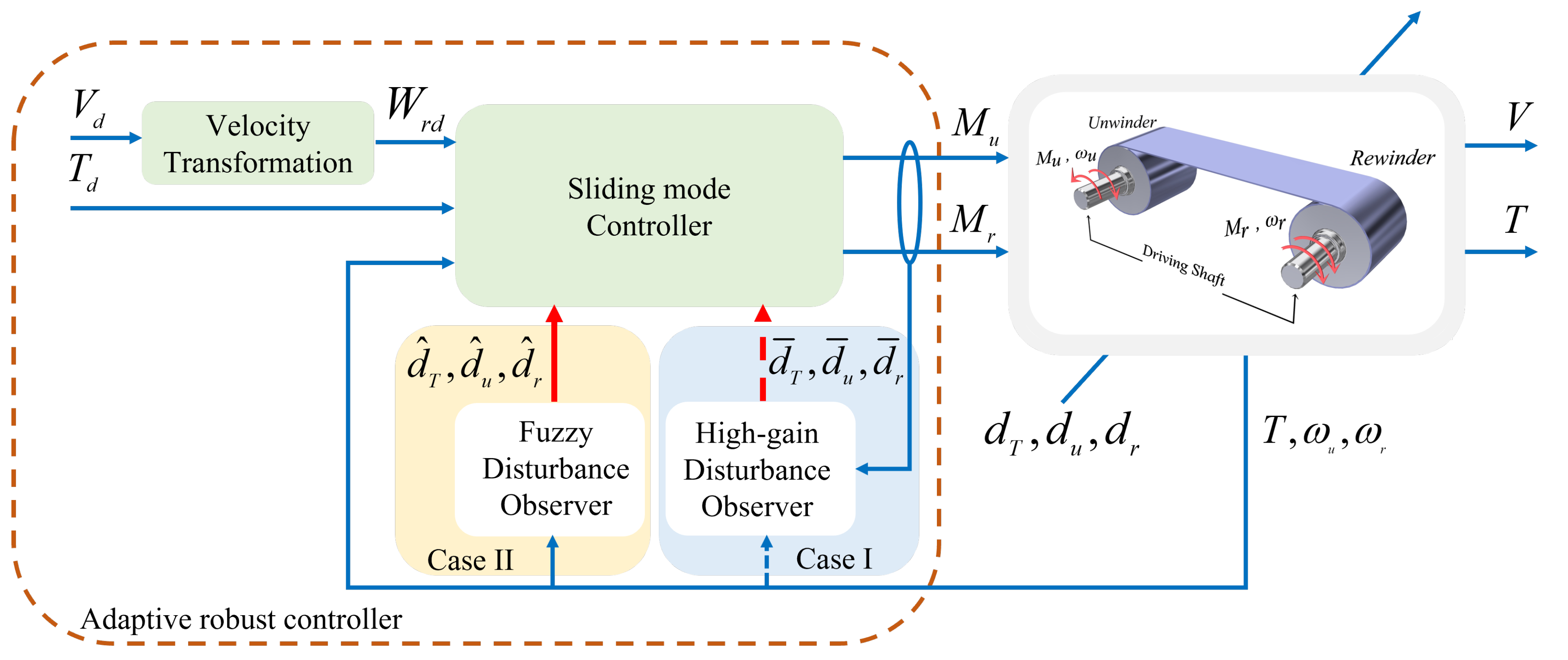
The sliding mode control which has been applied to the single-span roll-to-roll nonlinear system has robustness against model uncertainties and external disturbances. However, sliding mode control does not give a good response in case of high-amplitude disturbances. To increase the system’s adaptability to imprecision, an adaptive global sliding mode control method is developed for this system. Based on the control structure in Figure 4, we propose two algorithms: a high-gain disturbance observer and adaptive fuzzy algorithm for disturbance compensation.

4.1. High-Gain Disturbance Observer Design

From the mathematical model given in (21)–(23), we can see the appearance of the unknown disturbances $d_T,d_u,d_r$. To estimate these values and thus to improve the control system, the high-gain disturbance observer is proposed. Thus, Equations (21)–(23) are rewritten as follows:

$$d_T=\dot{T}-f_T-g_T{\omega }_u$$

(46)

$$d_u={\dot{\omega }}_u-f_u-g_u{M}_u$$

(47)

$$d_r={\dot{\omega }}_r-f_r-g_r{M}_r$$

(48)

We define the estimated variables as ${\overline{d}}_T,{\overline{d}}_u$ and ${\overline{d}}_r$. Then, the estimated deviation variables are defined as follows:

$$\begin{array}{cc}\hfill {\tilde{d}}_T& =d_T-{\overline{d}}_T\hfill \\ \hfill {\tilde{d}}_u& =d_u-{\overline{d}}_u\hfill \\ \hfill {\tilde{d}}_r& =d_r-{\overline{d}}_r\hfill \end{array}$$

(49)

The dynamic equations of the estimated variables are designed as follows:

$$\begin{array}{ccc}\hfill {\dot{\overline{d}}}_T& =& \frac{1}{{\epsilon }_T}\left(\dot{T}-f_T-g_T{\omega }_u-{\overline{d}}_T\right)\hfill \end{array}$$

(50)

$$\begin{array}{ccc}\hfill {\dot{\overline{d}}}_u& =& \frac{1}{{\epsilon }_u}\left({\dot{\omega }}_u-f_u-g_u{M}_u-{\overline{d}}_u\right)\hfill \end{array}$$

(51)

$$\begin{array}{ccc}\hfill {\dot{\overline{d}}}_r& =& \frac{1}{{\epsilon }_r}\left({\dot{\omega }}_r-f_r-g_r{M}_r-{\overline{d}}_r\right)\hfill \end{array}$$

(52)

In Equations (50)–(52), the state derivative is present, and thus the disturbance is amplified when using a high-gain disturbance observer. To solve the above problem, three auxiliary variables are used as follows:

$$\begin{array}{cc}\hfill {\chi }_T& ={\overline{d}}_T-\frac{T}{{\epsilon }_T}\hfill \\ \hfill {\chi }_u& ={\overline{d}}_u-\frac{{\omega }_u}{{\epsilon }_u}\hfill \\ \hfill {\chi }_r& ={\overline{d}}_r-\frac{{\omega }_r}{{\epsilon }_r}\hfill \end{array}$$

(53)

From Equations (50)–(53), the dynamic equations of the auxiliary state variables are obtained as follows:

$$\begin{array}{ccc}\hfill {\dot{\chi }}_T& =& -\frac{1}{{\epsilon }_T}\left({\chi }_T+\frac{T}{{\epsilon }_T}\right)-\frac{1}{{\epsilon }_T}\left(f_T+g_T{\omega }_u\right)\hfill \end{array}$$

(54)

$$\begin{array}{ccc}\hfill {\dot{\chi }}_u& =& -\frac{1}{{\epsilon }_u}\left({\chi }_u+\frac{{\omega }_u}{{\epsilon }_u}\right)-\frac{1}{{\epsilon }_u}\left(f_u+g_u{M}_u\right)\hfill \end{array}$$

(55)

$$\begin{array}{ccc}\hfill {\dot{\chi }}_r& =& -\frac{1}{{\epsilon }_r}\left({\chi }_r+\frac{{\omega }_r}{{\epsilon }_r}\right)-\frac{1}{{\epsilon }_r}\left(f_r+g_r{M}_r\right)\hfill \end{array}$$

(56)

Theorem 2.

For the nonlinear system of the web transport system (21)–(23), the bounded unknown disturbances shown in Equation (25) can be observed by using the high-gain disturbance observers that hold their form (54)–(56) with the auxiliary state variables (53).

Proof of Theorem 2.

The derivative of the auxiliary variables (53) with respect to time is given by

$$\begin{array}{c}\hfill {\dot{\chi }}_T={\dot{\overline{d}}}_T-\frac{\dot{T}}{{\epsilon }_T}\\ \hfill {\dot{\chi }}_u={\dot{\overline{d}}}_u-\frac{{\dot{\omega }}_u}{{\epsilon }_u}\\ \hfill {\dot{\chi }}_r={\dot{\overline{d}}}_r-\frac{{\dot{\omega }}_r}{{\epsilon }_r}\end{array}$$

(57)

From Equations (49) and (53)–(57), the following estimation error dynamic of the high-gain disturbance observers results in

$$\begin{array}{cc}\hfill {\dot{\tilde{d}}}_T& =-(1/{\epsilon }_T){\tilde{d}}_T+{\dot{d}}_T\hfill \\ \hfill {\dot{\tilde{d}}}_u& =-(1/{\epsilon }_u){\tilde{d}}_u+{\dot{d}}_u\hfill \\ \hfill {\dot{\tilde{d}}}_r& =-(1/{\epsilon }_r){\tilde{d}}_r+{\dot{d}}_r\hfill \end{array}$$

(58)

After some basic operations, it is straightforward to show that [30]

$$\begin{array}{cc}\hfill \left|{\tilde{d}}_T\right|& \le e^{-(1/{\epsilon }_T)t}\left|{\tilde{d}}_T\left(0\right)\right|+{\epsilon }_T{\rho }_T\left(t\right)\hfill \\ \hfill \left|{\tilde{d}}_r\right|& \le e^{-(1/{\epsilon }_r)t}\left|{\tilde{d}}_r\left(0\right)\right|+{\epsilon }_r{\rho }_r\left(t\right)\hfill \\ \hfill \left|{\tilde{d}}_u\right|& \le e^{-(1/{\epsilon }_u)t}\left|{\tilde{d}}_u\left(0\right)\right|+{\epsilon }_u{\rho }_u\left(t\right)\hfill \end{array}$$

(59)

where ${\rho }_T\left(t\right)$, ${\rho }_r\left(t\right)$, ${\rho }_u\left(t\right)$ denote the envelope functions, such that ${\rho }_T\left(t\right)\ge \left|{\dot{d}}_T\right|$, ${\rho }_r\left(t\right)\ge \left|{\dot{d}}_r\right|$, ${\rho }_u\left(t\right)\ge \left|{\dot{d}}_u\right|$, $\forall t\ge 0$. The upper bound of $|{\tilde{d}}_T\left(\infty \right)|,|{\tilde{d}}_r\left(\infty \right)|,|{\tilde{d}}_u\left(\infty \right)|$ becomes smaller when the observer gains $1/{\epsilon }_T,1/{\epsilon }_r,/1{\epsilon }_u$ are adjusted to be larger.

Remark 1.

The disturbance observers (54)–(56) with auxiliary state variables (53) do not need to use derivatives of the state variables $T,{\omega }_u,{\omega }_r$ as in Equations (50)–(52). Then, the measurement noise amplifications by using the high gains $1/{\epsilon }_T,1/{\epsilon }_r,1/{\epsilon }_u$ are reduced; thus, the observers are more feasible when applied in practice.

Combining the estimated values ${\overline{d}}_T,{\overline{d}}_u,{\overline{d}}_r$ from the high-gain disturbance observer, we rewrite the control signals as follows:

$$\begin{array}{ccc}\hfill {\overline{W}}_{ud}& =& \frac{1}{g_T}\left(-f_T-{\overline{d}}_T+{\dot{T}}_d-k_{T1}\mathrm{sgn}\left(S_T\right)-k_{T2}.S_T\right)\hfill \end{array}$$

(60)

$$\begin{array}{ccc}\hfill {\overline{M}}_u& =& \frac{1}{g_u}\left(-f_u-{\overline{d}}_u+{\dot{W}}_{ud}-k_{u1}\mathrm{sgn}\left(S_u\right)-k_{u2}.S_u\right)\hfill \end{array}$$

(61)

$$\begin{array}{ccc}\hfill {\overline{M}}_r& =& \frac{1}{g_r}\left(-f_r-{\overline{d}}_r+{\dot{W}}_{rd}-k_{r1}\mathrm{sgn}\left(S_r\right)-k_{r2}.S_r\right)\hfill \end{array}$$

(62)

Theorem 3.

Consider the web transport system described in detail in Equations (1)–(20) and rewritten in a general form as Equations (21)–(23) under an unknown disturbance bounded as given in Assumption 1; the control law (60)–(62) and the observer gains ${\epsilon }_T,{\epsilon }_u,{\epsilon }_r$ of the high-gain disturbance observer (54)–(56) with the auxiliary state variables (53) guarantee the input-to-state stability [31] of the control system.

Proof of Theorem 3.

Define Lyapunov candidate function $V_2$ as

$$V_2=\frac{1}{2}{S}_T^2+\frac{1}{2}{S}_u^2+\frac{1}{2}{S}_r^2+\frac{1}{2}{\tilde{d}}_T^2+\frac{1}{2}{\tilde{d}}_u^2+\frac{1}{2}{\tilde{d}}_r^2$$

(63)

Substituting Equations (58) and (60)–(62) into the derivative of Lyapunov candidate function $V_2$ with respect to time,

$$\begin{array}{cc}\hfill \dot{V_2}=& -\left(k_{T1}\left|S_T\right|+k_{T2}.S_T^2+{\tilde{d}}_T{S}_T\right)-\left(k_{u1}\left|S_u\right|+k_{u2}.S_u^2+{\tilde{d}}_u{S}_u\right)\hfill \\ \hfill & -\left(k_{r1}\left|S_r\right|+k_{r2}.S_r^2+{\tilde{d}}_r{S}_r\right)-\frac{1}{{\epsilon }_T}{\tilde{d}}_T^2+{\tilde{d}}_T{\dot{d}}_T-\frac{1}{{\epsilon }_u}{\tilde{d}}_u^2+{\tilde{d}}_u{\dot{d}}_u-\frac{1}{{\epsilon }_r}{\tilde{d}}_r^2+{\tilde{d}}_r{\dot{d}}_r\hfill \end{array}$$

(64)

Applying the inequality $\left|x\right|\left|y\right|⩾xy$ into Equation (64), we obtain

$$\begin{array}{cc}\hfill \dot{V_2}\le & -\left(k_{T2}.S_T^2+{\tilde{d}}_T{S}_T+\frac{1}{{\epsilon }_T}{\tilde{d}}_T^2-|{\tilde{d}}_T\left|\right|{\dot{d}}_T|\right)-\left(k_{u2}.S_u^2+{\tilde{d}}_u{S}_u+\frac{1}{{\epsilon }_u}{\tilde{d}}_u^2-|{\tilde{d}}_u\left|\right|{\dot{d}}_u|\right)\hfill \\ \hfill & -\left(k_{r2}.S_r^2+{\tilde{d}}_r{S}_r+\frac{1}{{\epsilon }_r}{\tilde{d}}_r^2-|{\tilde{d}}_r\left|\right|{\dot{d}}_r|\right)\hfill \end{array}$$

(65)

Then,

$$\begin{array}{cc}\hfill \dot{V_2}\le & -k_{T2}{\left(\frac{S_T}{{\alpha }_T}-\frac{{\alpha }_T}{2k_{T2}}{\tilde{d}}_T\right)}^2-{\tau }_T{\left(|{\tilde{d}}_T|-\frac{1}{2{\tau }_T}\left|{\dot{d}}_T\right|\right)}^2-\left(1-\frac{1}{{\alpha }_T^2}\right)k_{T2}{S}_T^2-\frac{{\beta }_T^2}{4k_{T2}}{\tilde{d}}_T^2\hfill \\ \hfill & -k_{u2}{\left(\frac{S_u}{{\alpha }_u}-\frac{{\alpha }_u}{2k_{u2}}{\tilde{d}}_u\right)}^2-{\tau }_u{\left(|{\tilde{d}}_u|-\frac{1}{2{\tau }_u}\left|{\dot{d}}_u\right|\right)}^2-\left(1-\frac{1}{{\alpha }_u^2}\right)k_{u2}{S}_u^2-\frac{{\beta }_u^2}{4k_{u2}}{\tilde{d}}_u^2\hfill \\ \hfill & -k_{r2}{\left(\frac{S_r}{{\alpha }_r}-\frac{{\alpha }_r}{2k_{r2}}{\tilde{d}}_r\right)}^2-{\tau }_r{\left(|{\tilde{d}}_r|-\frac{1}{2{\tau }_r}\left|{\dot{d}}_r\right|\right)}^2-\left(1-\frac{1}{{\alpha }_r^2}\right)k_{r2}{S}_r^2-\frac{{\beta }_r^2}{4k_{r2}}{\tilde{d}}_r^2\hfill \\ \hfill & +\frac{1}{4{\tau }_r}{{\dot{d}}_{T,max}}^2+\frac{1}{4{\tau }_r}{{\dot{d}}_{u,max}}^2+\frac{1}{4{\tau }_i}{{\dot{d}}_{r,max}}^2\hfill \end{array}$$

(66)

where

$$\begin{array}{cc}\hfill {\tau }_T& =\left(\frac{1}{{\epsilon }_T}-\frac{{\alpha }_T^2+{\beta }_T^2}{4k_{T2}}\right),{\tau }_u=\left(\frac{1}{{\epsilon }_u}-\frac{{\alpha }_u^2+{\beta }_u^2}{4k_{u2}}\right),{\tau }_r=\left(\frac{1}{{\epsilon }_r}-\frac{{\alpha }_r^2+{\beta }_r^2}{4k_{r2}}\right)\hfill \\ \hfill {\alpha }_T& ,{\alpha }_u,{\alpha }_r>1;{\beta }_T,{\beta }_u,{\beta }_r\ne 0\hfill \end{array}$$

The following constants are found:

$$\begin{array}{c}\hfill \left\{\begin{array}{c}\varsigma =\frac{1}{4{\tau }_r}{\dot{d}}_{T,max}^2+\frac{1}{4{\tau }_r}{\dot{d}}_{u,max}^2+\frac{1}{4{\tau }_i}{\dot{d}}_{r,max}^2\hfill \\ \lambda =min\left\{\left(1-\frac{1}{{\alpha }_T^2}\right)k_{T2},\left(1-\frac{1}{{\alpha }_u^2}\right)k_{u2},\left(1-\frac{1}{{\alpha }_r^2}\right)k_{r2},\frac{{\beta }_T^2}{4k_{T2}},\frac{{\beta }_u^2}{4k_{u2}},\frac{{\beta }_r^2}{4k_{r2}}\right\}\hfill \end{array}\right.\end{array}$$

(67)

Then, we obtain

$$\begin{array}{c}\hfill {\dot{V}}_2⩽-2\lambda V_2+\varsigma \end{array}$$

(68)

Consequently,

$$V_2\left(t\right)⩽V_2\left(0\right)e^{-2\lambda t}+\frac{\varsigma }{2\lambda }\left(1-e^{-2\lambda t}\right)$$

(69)

The inequality (69) shows that $V_2⩽\varkappa$ when $t\to \infty$, in which the value of $\varkappa$ depends on $\frac{\varsigma }{2\lambda }$. □

Remark 2.

Equation (69) implies that the tracking errors $S_T,S_u,S_r$ and estimation errors ${\tilde{d}}_T,{\tilde{d}}_u,{\tilde{d}}_r$ of the web transport system using high-gain disturbance observers exponentially converge to an arbitrarily small ball $\frac{\varsigma }{2\lambda }$ whose radius can be shrunk by ς via the high observer gains $1/{\epsilon }_T,1/{\epsilon }_r,1/{\epsilon }_u$.

4.2. Fuzzy Disturbance Observer

To eliminate disturbance in the single-span roll-to-roll system, the control signals in (38)–(40) are rewritten as follows:

$$\begin{array}{ccc}\hfill {\widehat{W}}_{ud}& =& \frac{1}{g_T}\left(-f_T+{\dot{T}}_d-{\widehat{d}}_T-k_{T1}\mathrm{sgn}\left(S_T\right)-k_{T2}.S_T\right)\hfill \end{array}$$

(70)

$$\begin{array}{ccc}\hfill {\widehat{M}}_u& =& \frac{1}{g_u}\left(-f_u+{\dot{W}}_{ud}-{\widehat{d}}_u-k_{u1}\mathrm{sgn}\left(S_u\right)-k_{u2}.S_u\right)\hfill \end{array}$$

(71)

$$\begin{array}{ccc}\hfill {\widehat{M}}_r& =& \frac{1}{g_r}\left(-f_r+{\dot{W}}_{rd}-{\widehat{d}}_r-k_{r1}\mathrm{sgn}\left(S_r\right)-k_{r2}.S_r\right)\hfill \end{array}$$

(72)

where the estimated variables ${\widehat{d}}_T,{\widehat{d}}_{\omega u}$, and ${\widehat{d}}_{\omega r}$ are computed directly by using a fuzzy disturbance observer as the control structure in Figure 5 to approximate effectively the disturbances $d_T,d_{\omega u}$, and $d_{\omega r}$. In this structure, we design the inputs of the fuzzy logic block to be only the sliding surfaces defined in (26)–(28). The fuzzy rules are defined as follows:

$$\begin{array}{cc}\hfill & \mathrm{If}{S}_T\mathrm{is}{s}_{Ti}\mathrm{then}{\widehat{d}}_{Ti}={\widehat{D}}_{Ti};i=\overline{1\cdots n}\hfill \\ \hfill & \mathrm{If}{S}_u\mathrm{is}{s}_{ui}\mathrm{then}{\widehat{d}}_{ui}={\widehat{D}}_{ui};i=\overline{1\cdots n}\hfill \\ \hfill & \mathrm{If}{S}_r\mathrm{is}{s}_{ri}\mathrm{then}{\widehat{d}}_{ri}={\widehat{D}}_{ri};i=\overline{1\cdots n}\hfill \end{array}$$

(73)

where $s_{Ti}$, $s_{ui}$ and $s_{ri}$ are fuzzy sets whose membership functions could be properly chosen, and ${\widehat{D}}_{Ti}$, ${\widehat{D}}_{ui}$, and ${\widehat{D}}_{ri}$ are the output value of each one of the n fuzzy rules, respectively. Considering that each rule defines a numerical value as outputs ${\widehat{D}}_{Ti}$, ${\widehat{D}}_{ui}$, and ${\widehat{D}}_{ri}$, the final outputs ${\widehat{d}}_T$, ${\widehat{d}}_u$, and ${\widehat{d}}_r$, respectively, can be computed by a weighted average:

$$\begin{array}{cc}& {\widehat{d}}_T={\widehat{\mathbf{D}}}_T^T{\mathsf{\Lambda }}_T\end{array}$$

(74)

$$\begin{array}{cc}& {\widehat{d}}_u={\widehat{\mathbf{D}}}_u^T{\mathsf{\Lambda }}_u\end{array}$$

(75)

$$\begin{array}{cc}& {\widehat{d}}_r={\widehat{\mathbf{D}}}_r^T{\mathsf{\Lambda }}_r\end{array}$$

(76)

where ${\widehat{\mathbf{D}}}_T=\left[{\widehat{D}}_{T1},{\widehat{D}}_{T2},\cdots ,{\widehat{D}}_{Tn}\right]$, ${\widehat{\mathbf{D}}}_u=\left[{\widehat{D}}_{u1},{\widehat{D}}_{u2},\cdots ,{\widehat{D}}_{un}\right]$, and ${\widehat{\mathbf{D}}}_r=\left[{\widehat{D}}_{r1},{\widehat{D}}_{r2},\cdots ,{\widehat{D}}_{rn}\right]$, respectively, are vectors containing the attributed values ${\widehat{D}}_{Ti}$, ${\widehat{D}}_{ui}$, and ${\widehat{D}}_{ri}$ to each rule i; define ${\mathsf{\Lambda }}_T=\left[{\kappa }_{T1},{\kappa }_{T2},\cdots ,{\kappa }_{Tn}\right]$, ${\mathsf{\Lambda }}_u=\left[{\kappa }_{u1},{\kappa }_{u2},\cdots ,{\kappa }_{un}\right]$, and ${\mathsf{\Lambda }}_r=\left[{\kappa }_{r1},{\kappa }_{r2},\cdots ,{\kappa }_{rn}\right]$, respectively, are vectors with components ${\kappa }_{Ti}={\zeta }_{Ti}/{\displaystyle \sum _{i=1}^n}{\zeta }_{Ti}$, ${\kappa }_{ui}={\zeta }_{ui}/{\displaystyle \sum _{i=1}^n}{\zeta }_{ui}$, and ${\kappa }_{ri}={\zeta }_{ri}/{\displaystyle \sum _{i=1}^n}{\zeta }_{ri}$; ${\zeta }_{ui}$, ${\zeta }_{ui}$, and ${\zeta }_{ui}$ are the firing strengths of each rule in (73). We propose that the vector of adjustable parameters can be automatically updated by the following adaptation laws to ensure the best possible estimation.

$$\begin{array}{cc}& {\dot{\widehat{\mathbf{D}}}}_T={\sigma }_1{S}_T{\mathsf{\Lambda }}_T\end{array}$$

(77)

$$\begin{array}{cc}& {\dot{\widehat{\mathbf{D}}}}_u={\sigma }_2{S}_u{\mathsf{\Lambda }}_u\end{array}$$

(78)

$$\begin{array}{cc}& {\dot{\widehat{\mathbf{D}}}}_r={\sigma }_3{S}_r{\mathsf{\Lambda }}_r\end{array}$$

(79)

where ${\sigma }_1,{\sigma }_2$, and ${\sigma }_3$ are strictly positive constants related to the adaptation rate.

Theorem 4.

Consider the single-span roll-to-roll nonlinear system described in detail in Equations (21)–(23) and bounded unknown disturbance mentioned in Assumption 1. Then, the system obtains stability according to the Lyapunov theorem by using the control signals (70)–(72) and adaptive laws in (77)–(79).

Proof of Theorem 4.

Let a positive-definite Lyapunov function candidate $V_3$ be defined as

$$V_3=\frac{1}{2}{S}_T+\frac{1}{2}{S}_u^2+\frac{1}{2}{S}_r^2+\frac{1}{2{\sigma }_1}{\mathsf{\Omega }}_T^T{\mathsf{\Omega }}_T+\frac{1}{2{\sigma }_2}{\mathsf{\Omega }}_u^T{\mathsf{\Omega }}_u+\frac{1}{2{\sigma }_3}{\mathsf{\Omega }}_r^T{\mathsf{\Omega }}_r$$

(80)

where ${\mathsf{\Omega }}_T={\widehat{\mathbf{D}}}_{\mathbf{T}}-{\widehat{\mathbf{D}}}_T^{*}$, ${\mathsf{\Omega }}_u={\widehat{\mathbf{D}}}_{\mathbf{u}}-{\widehat{\mathbf{D}}}_u^{*}$, ${\mathsf{\Omega }}_r={\widehat{\mathbf{D}}}_{\mathbf{r}}-{\widehat{\mathbf{D}}}_r^{*}$ and ${\widehat{\mathbf{D}}}_T^{*}$, ${\widehat{\mathbf{D}}}_u^{*}$, ${\widehat{\mathbf{D}}}_r^{*}$ are the optimal parameter vectors, associated with the optimal estimates ${\widehat{d}}_T^{*}$, ${\widehat{d}}_u^{*}$, ${\widehat{d}}_r^{*}$, respectively. Taking the derivative with respect to time,

$$\begin{array}{cc}\hfill \dot{V_3}& =S_T{\dot{S}}_T+S_u{\dot{S}}_u+S_r{\dot{S}}_r+\frac{1}{{\sigma }_1}{\mathsf{\Omega }}_T^T{\dot{\mathsf{\Omega }}}_T+\frac{1}{{\sigma }_2}{\mathsf{\Omega }}_u^T{\dot{\mathsf{\Omega }}}_u+\frac{1}{{\sigma }_3}{\mathsf{\Omega }}_r^T{\dot{\mathsf{\Omega }}}_r\hfill \\ \hfill & =S_T\left(f_T+g_T{\omega }_u+d_T-{\dot{T}}_d\right)+S_u\left(f_u+g_u{M}_u+d_u-{\dot{W}}_{ud}\right)\hfill \\ \hfill & +S_r\left(f_r+g_r{M}_r+d_r-{\dot{W}}_{rd}\right)+\frac{1}{{\sigma }_1}{\mathsf{\Omega }}_T^T{\dot{\mathsf{\Omega }}}_T+\frac{1}{{\sigma }_2}{\mathsf{\Omega }}_u^T{\dot{\mathsf{\Omega }}}_u+\frac{1}{{\sigma }_3}{\mathsf{\Omega }}_r^T{\dot{\mathsf{\Omega }}}_r\hfill \end{array}$$

(81)

Substituting the control signals rewritten in (70)–(72) into (81), we obtain

$$\begin{array}{cc}\hfill \dot{V_3}& =\frac{1}{{\sigma }_1}{\mathsf{\Omega }}_T^T{\dot{\mathsf{\Omega }}}_T+\frac{1}{{\sigma }_2}{\mathsf{\Omega }}_u^T{\dot{\mathsf{\Omega }}}_u+\frac{1}{{\sigma }_3}{\mathsf{\Omega }}_r^T{\dot{\mathsf{\Omega }}}_r+S_T\left(d_T-{\widehat{d}}_T-k_{T1}\mathrm{sgn}\left(S_T\right)-k_{T2}.S_T\right)\hfill \\ \hfill & +S_u\left(d_u-{\widehat{d}}_u-k_{u1}\mathrm{sgn}\left(S_u\right)-k_{u2}.S_u\right)+S_r\left(d_r-{\widehat{d}}_r-k_{r1}\mathrm{sgn}\left(S_r\right)-k_{r2}.S_r\right)\hfill \end{array}$$

(82)

Defining the minimum approximation errors as ${\alpha }_T={\widehat{d}}_T^{*}-d_T$, ${\alpha }_u={\widehat{d}}_u^{*}-d_u$, ${\alpha }_r={\widehat{d}}_r^{*}-d_r$ and noting that ${\dot{\mathsf{\Omega }}}_T={\dot{\widehat{\mathbf{D}}}}_{\mathbf{T}}$, ${\dot{\mathsf{\Omega }}}_u={\dot{\widehat{\mathbf{D}}}}_{\mathbf{u}}$, ${\dot{\mathsf{\Omega }}}_r={\dot{\widehat{\mathbf{D}}}}_{\mathbf{r}}$, Equation (82) becomes

$$\begin{array}{cc}\hfill \dot{V_3}& =\frac{1}{{\sigma }_1}{\mathsf{\Omega }}_T^T{\dot{\widehat{\mathbf{D}}}}_T-S_T\left({\alpha }_T+{\widehat{d}}_T-{\widehat{d}}_T^{*}+k_{T1}\mathrm{sgn}\left(S_T\right)+k_{T2}{S}_T\right)\hfill \\ \hfill & +\frac{1}{{\sigma }_2}{\mathsf{\Omega }}_u^T{\dot{\widehat{\mathbf{D}}}}_u-S_u\left({\alpha }_u+{\widehat{d}}_u-{\widehat{d}}_u^{*}+k_{u1}\mathrm{sgn}\left(S_u\right)+k_{u2}{S}_u\right)\hfill \\ \hfill & +\frac{1}{{\sigma }_3}{\mathsf{\Omega }}_r^T{\dot{\widehat{\mathbf{D}}}}_r-S_r\left({\alpha }_r+{\widehat{d}}_r-{\widehat{d}}_r^{*}+k_{r1}\mathrm{sgn}\left(S_r\right)+k_{r2}{S}_r\right)\hfill \\ \hfill & =\frac{1}{{\sigma }_1}{\mathsf{\Omega }}_T^T\left({\dot{\widehat{\mathbf{D}}}}_T-{\sigma }_1{S}_T{\mathsf{\Lambda }}_T\right)-S_T\left({\alpha }_T+k_{T1}\mathrm{sgn}\left(S_T\right)+k_{T2}{S}_T\right)\hfill \\ \hfill & +\frac{1}{{\sigma }_2}{\mathsf{\Omega }}_u^T\left({\dot{\widehat{\mathbf{D}}}}_u-{\sigma }_2{S}_u{\mathsf{\Lambda }}_u\right)-S_u({\alpha }_u+k_{u1}\mathrm{sgn}\left(S_u)+k_{u2}{S}_u\right)\hfill \\ \hfill & +\frac{1}{{\sigma }_3}{\mathsf{\Omega }}_r^T\left({\dot{\widehat{\mathbf{D}}}}_r-{\sigma }_3{S}_r{\mathsf{\Lambda }}_r\right)-S_r\left({\alpha }_r+k_{r1}\mathrm{sgn}\left(S_r\right)+k_{r2}{S}_r\right)\hfill \end{array}$$

(83)

By applying the adaptation laws in (77)–(79) for ${\dot{\widehat{\mathbf{D}}}}_T$, ${\dot{\widehat{\mathbf{D}}}}_u$ and ${\dot{\widehat{\mathbf{D}}}}_r$, we rewrite ${\dot{V}}_3$ as follows:

$$\begin{array}{c}\hfill \dot{V_3}=-k_{T2}{S}_T^2-k_{u2}{S}_u^2-k_{r2}{S}_r^2-S_T{\alpha }_T-k_{T1}\left|S_T\right|-S_u{\alpha }_u-k_{u1}\left|S_u\right|-S_r{\alpha }_r-k_{r1}\left|S_r\right|\end{array}$$

(84)

Furthermore, it can be seen that

$$\begin{array}{cc}\hfill & \left|{\alpha }_T\right|=\left|{\widehat{d}}_T^{*}-d_T\right|\le \left|{\widehat{d}}_T-d_T\right|\le \left|{\widehat{d}}_T\right|+{\delta }_1\hfill \\ \hfill & \left|{\alpha }_u\right|=\left|{\widehat{d}}_u^{*}-d_u\right|\le \left|{\widehat{d}}_u^{}-d_u\right|\le \left|{\widehat{d}}_u\right|+{\delta }_2\hfill \\ \hfill & \left|{\alpha }_r\right|=\left|{\widehat{d}}_r^{*}-d_r\right|\le \left|{\widehat{d}}_r^{}-d_r\right|\le \left|{\widehat{d}}_r\right|+{\delta }_3\hfill \end{array}$$

(85)

The control parameters are chosen as $k_{T1}\ge \left|{\widehat{d}}_T\right|+{\delta }_1$, $k_{u1}\ge \left|{\widehat{d}}_u\right|+{\delta }_2$, $k_{r1}\ge \left|{\widehat{d}}_r\right|+{\delta }_3$, and $k_{T2}$, $k_{u2}$, $k_{r2}$ are strictly positive constants; thus, it can be concluded that $\dot{V_3}\le 0$. □

Remark 3.

To deal with the imprecise single-span roll-to-roll nonlinear system, adaptive fuzzy sliding mode control is an effective solution because the fuzzy disturbance observer does not need model information. The control law in (70)–(72) actually ensures not only the finite-time convergence to a sliding surface but also the asymptotic stability of the closed-loop system, while the control law in (60)–(62) using a high-gain disturbance observer only drives the system converge to an arbitrarily small ball.

5. Simulation Results

In this section, the performance of the proposed controller is demonstrated through simulations. The parameters of the roll-to-roll system utilized in the simulation can be listed as follows: $R_{u0}=0.1\mathrm{m};R_{r0}=0.05\mathrm{m};J_{u0}=1.5{\mathrm{kgm}}^2;{\mathrm{J}}_{\mathrm{r}0}=1{\mathrm{kgm}}^2;\mathrm{L}=0.3\mathrm{m};$ $w=0.3\mathrm{m};$ $b_{fu}=b_{fr}=0.00002533\mathrm{Nms};E=2.5\times {10}^9\mathrm{N}/{\mathrm{m}}^2$. The controller parameters are calculated as follows: $k_{T1}=k_{u1}=k_{r1}=5;k_{T2}=k_{u2}=k_{r2}=100;$${\epsilon }_T={\epsilon }_u={\epsilon }_r=0.001$.

The cause of the chattering effect is that the sign function is actually used instead of the ideal sign function in (33). To eliminate chattering, we propose replacing the sign function with the saturation function. This function is in continuous form and is only meaningful to reduce the frequency of the sign switching of the control signal, but not the amplitude of the oscillation. In this section, we compare the control performance among three control algorithms: sliding mode control (SMC) with a saturation function, a high-gain disturbance observer, and the adaptive fuzzy algorithm.

We conduct the simulation with $d_T=0.9sin\left(3t\right)$, $d_u=0.3sin\left(3t\right)$, and $d_r=0.6sin\left(3t\right)$. Results are presented in the figures below.

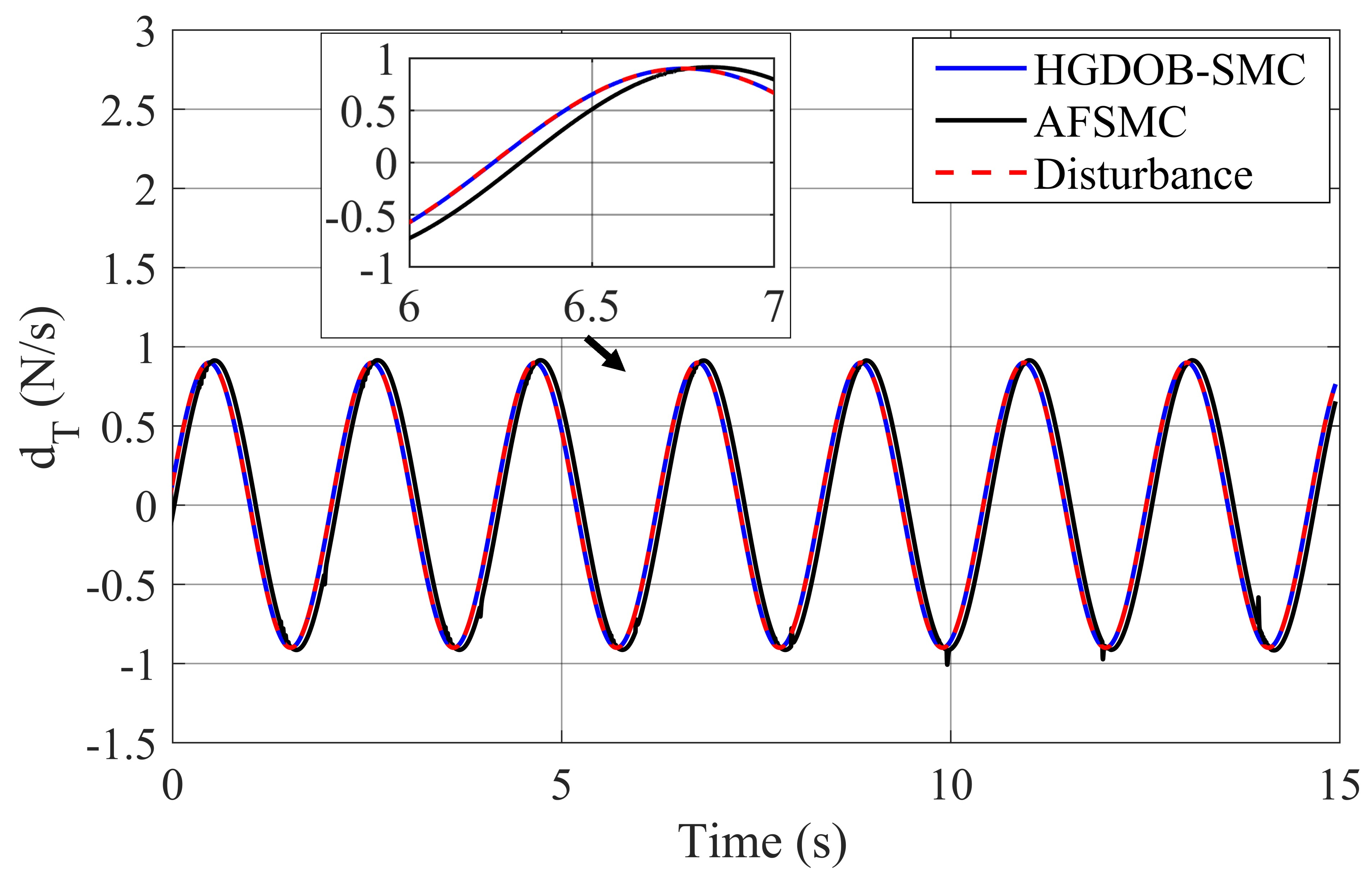
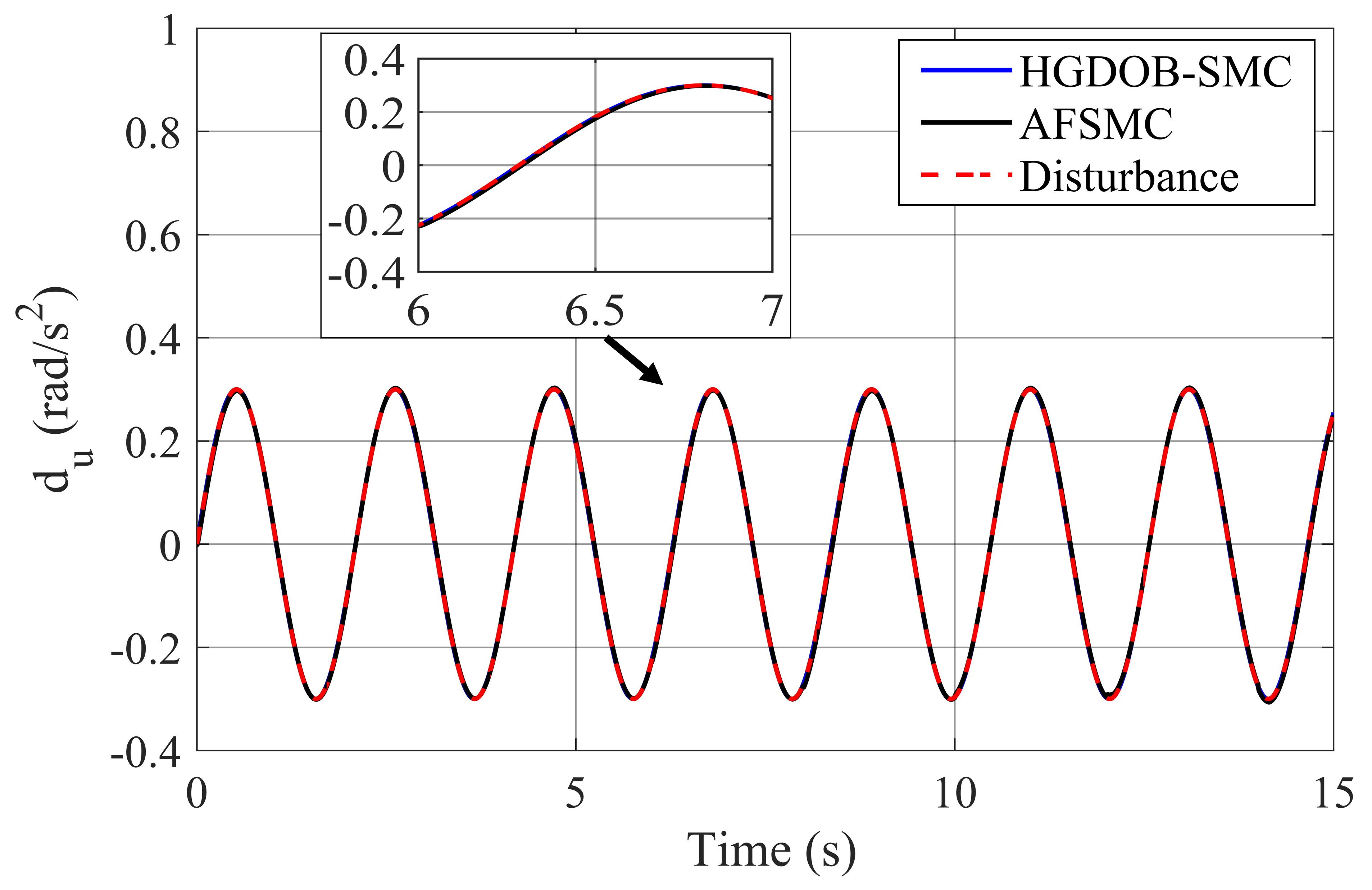
The disturbance estimation results are presented in Figure 5, Figure 6 and Figure 7 based on the high-gain disturbance observer in Equations (54)–(56) and the adaptive fuzzy laws in Equations (77)–(79). It can be verified that the proposed control law provides good performance.

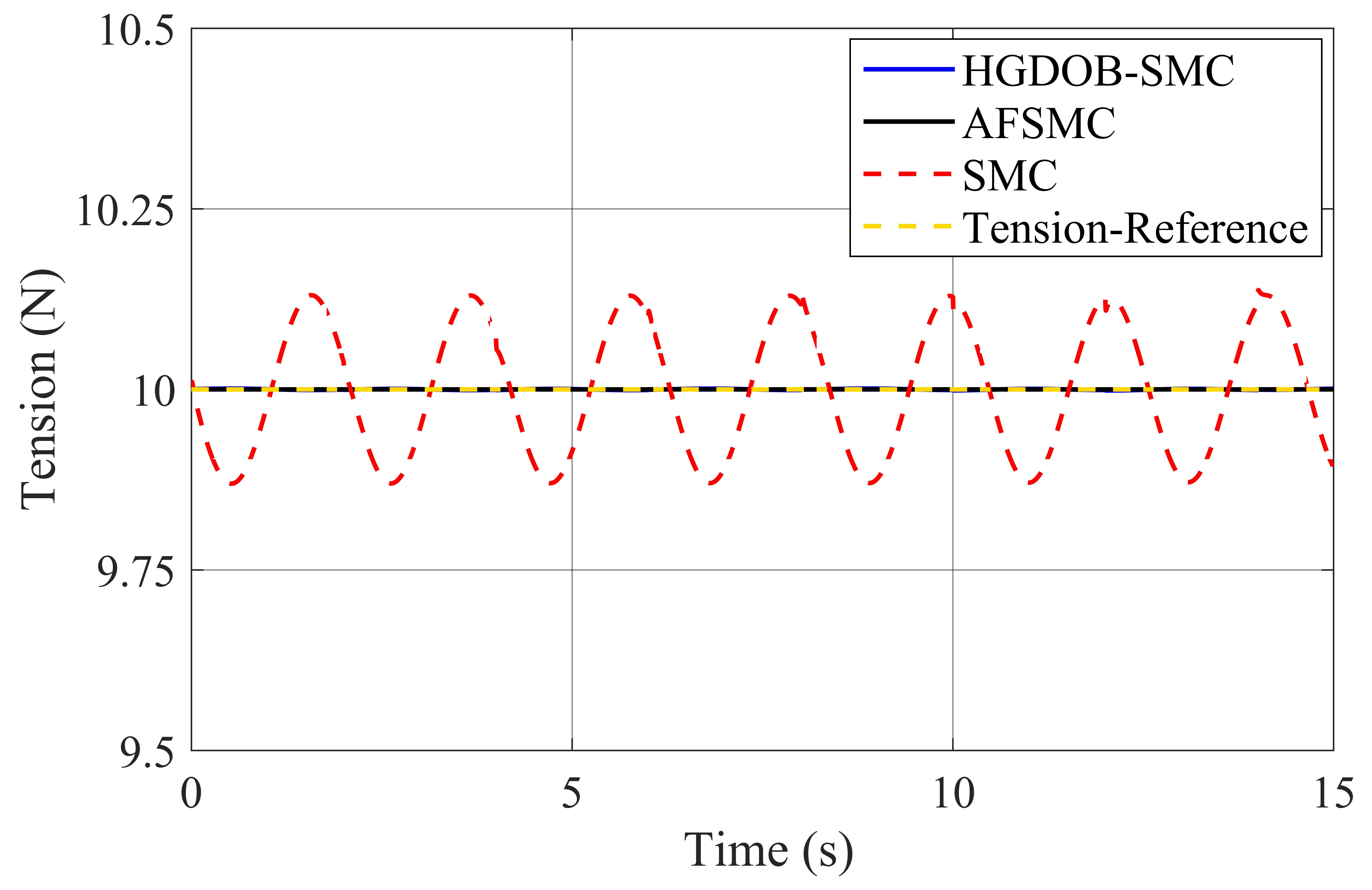
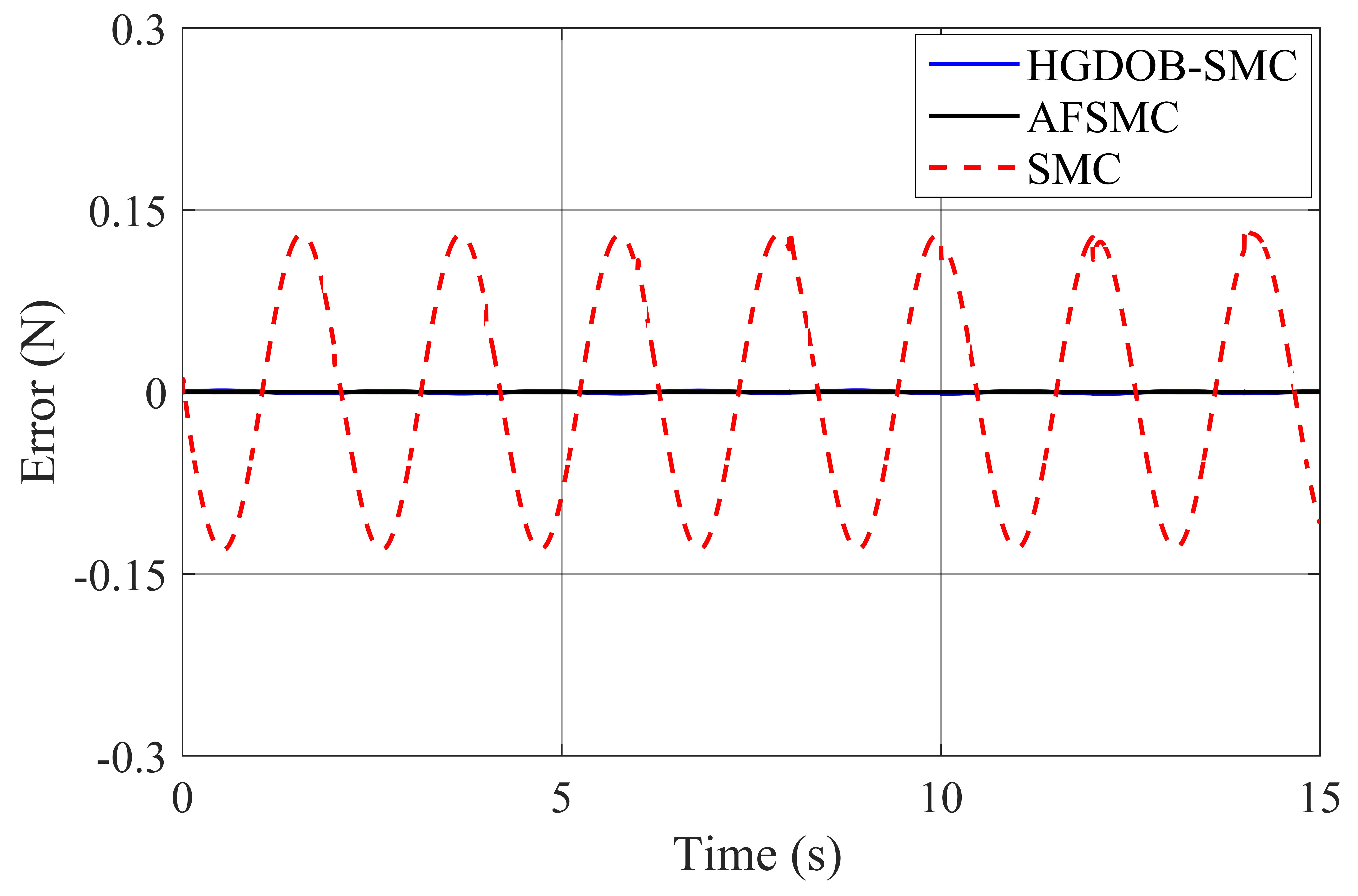
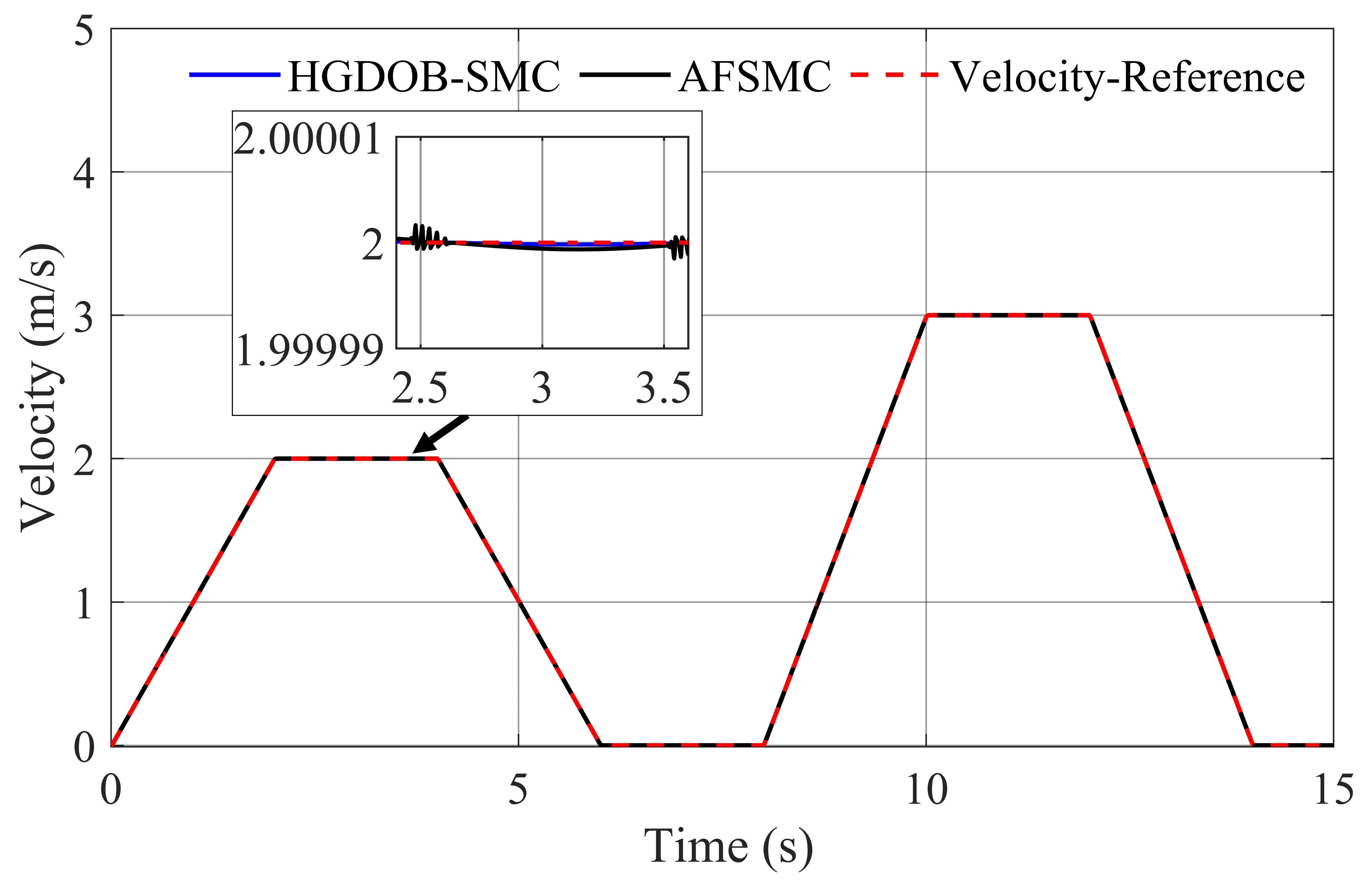
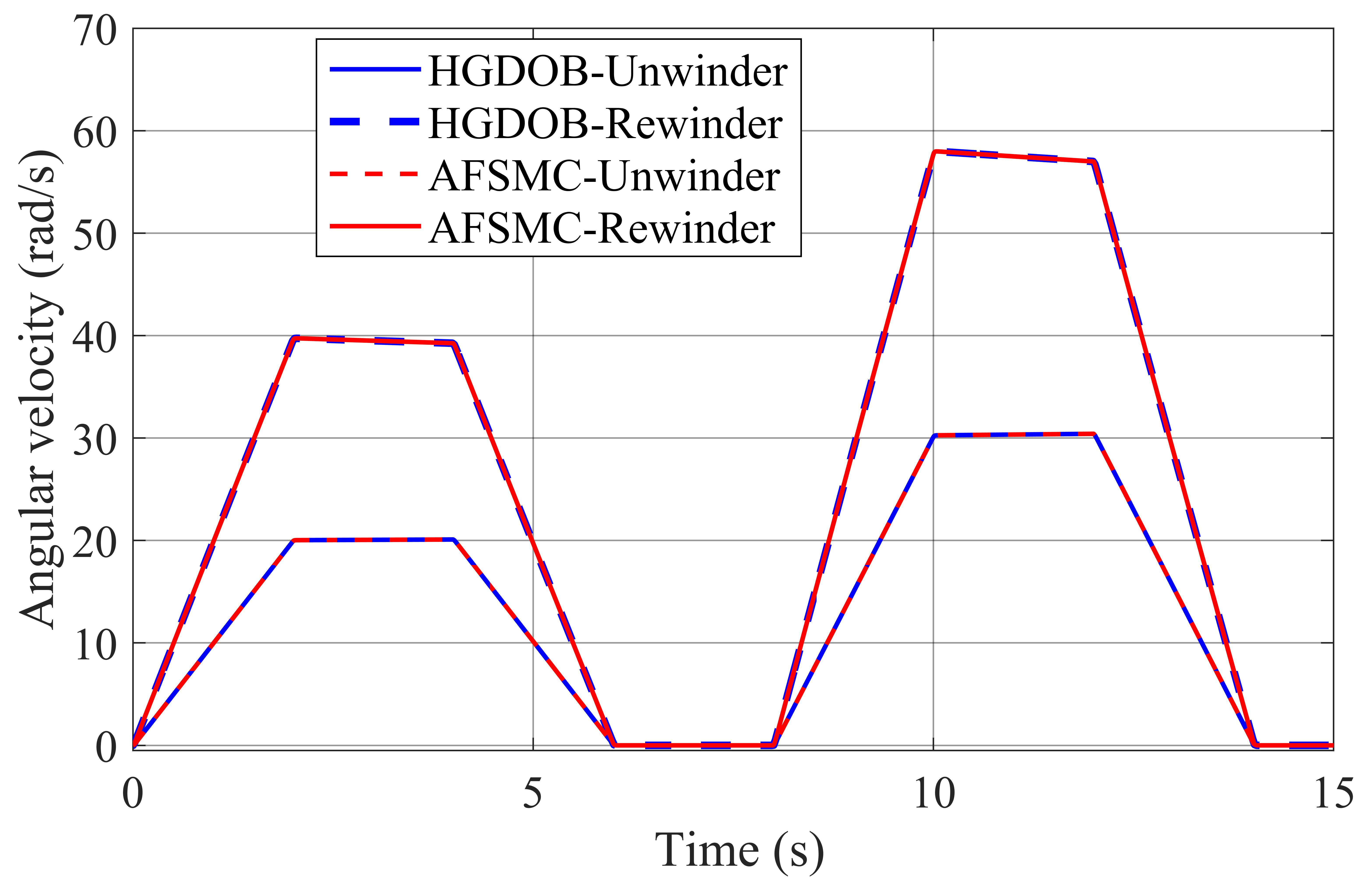
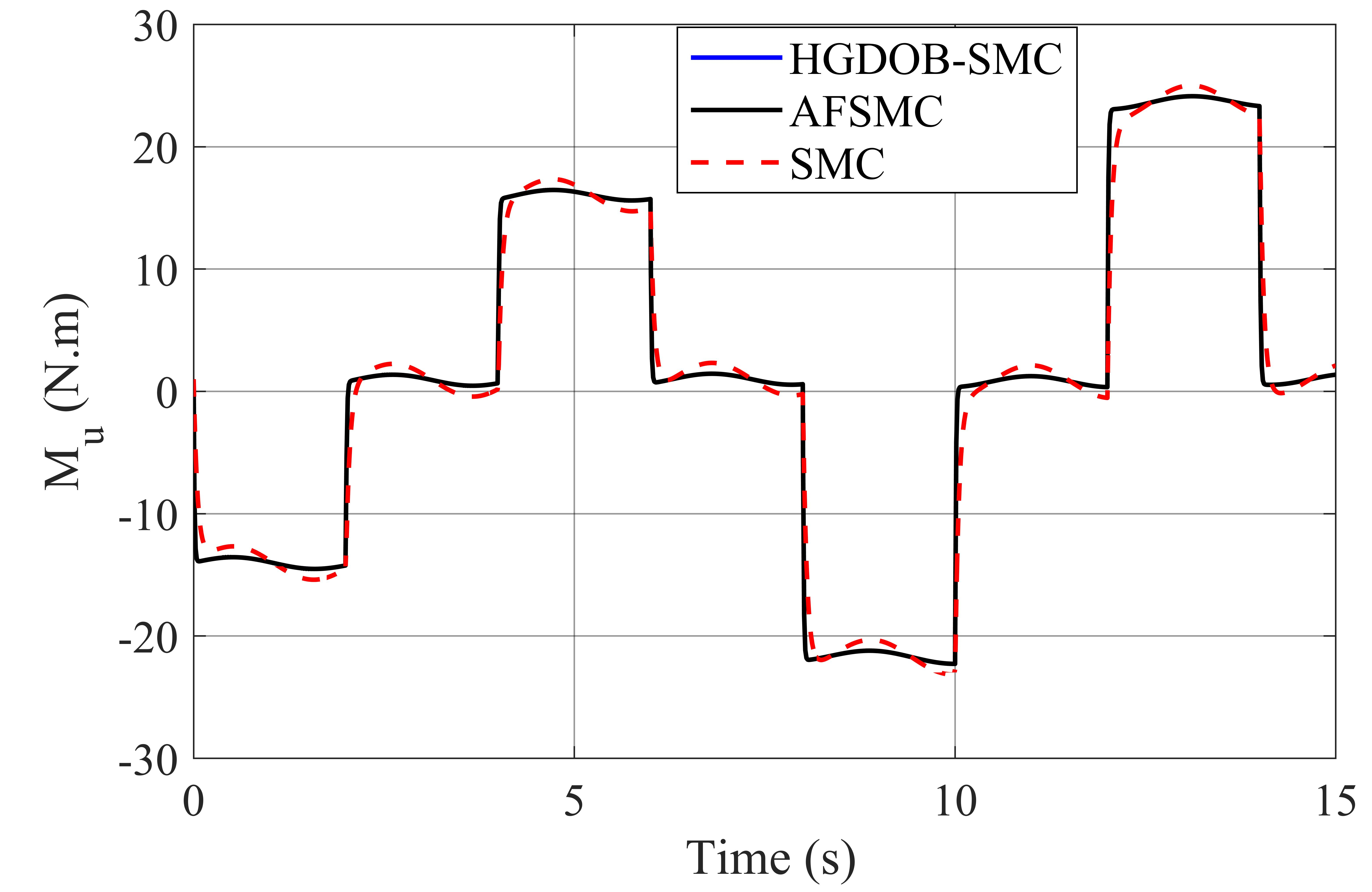
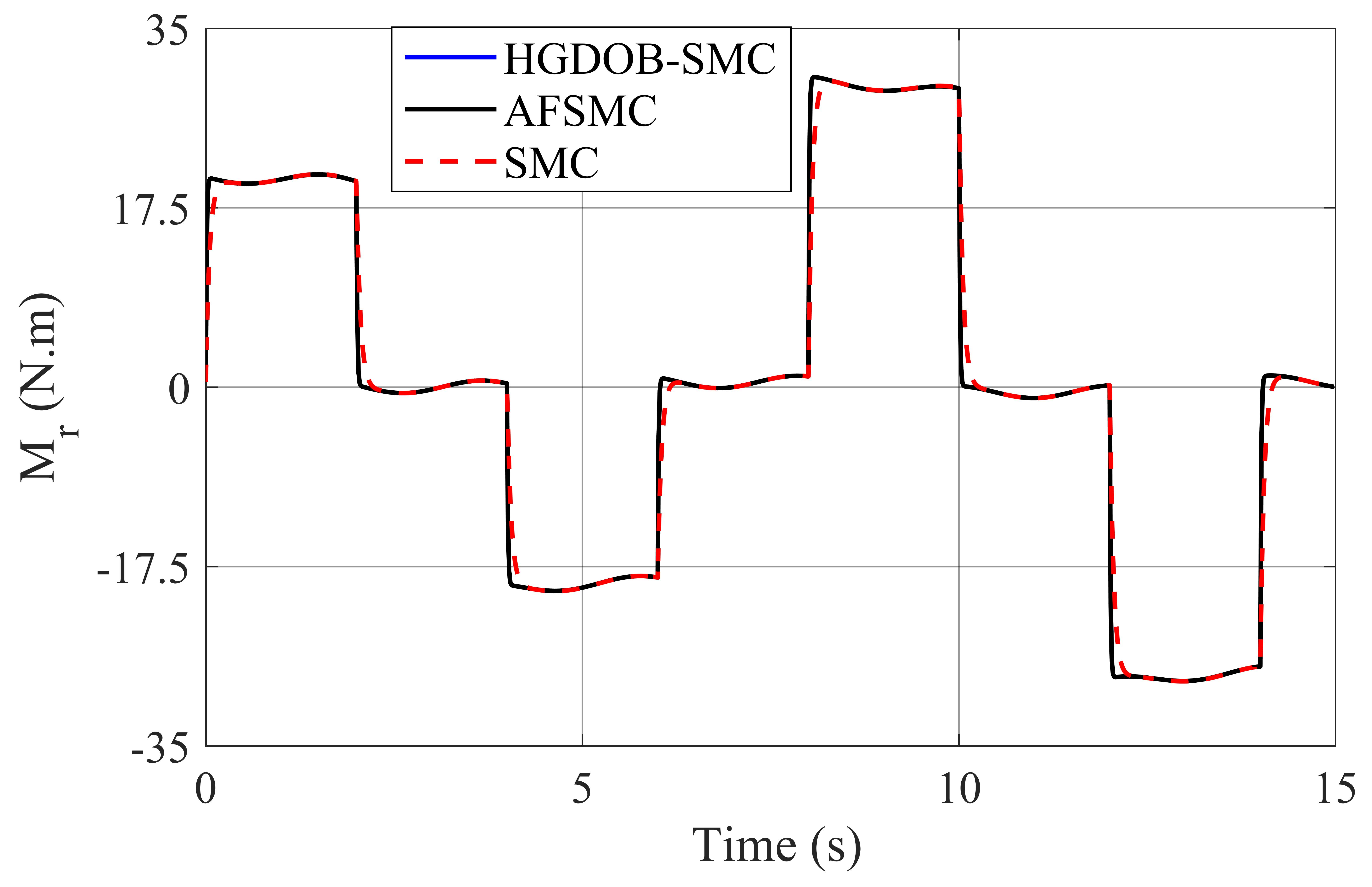
In Figure 8, Figure 9 and Figure 10, the proposed controllers help the tension and velocity responses to track the set value with almost negligible error. However, replacing the sign function by a saturation function can minimize or, when desired, even completely eliminate chattering, but this turns perfect tracking into a tracking with a guaranteed precision problem, which actually means that a steady-state error will always remain. The improved performance of AFSMC (adaptive fuzzy sliding mode control) and the HGDOB (high-gain disturbance observer) over sliding mode control (SMC) is due to its ability to recognize and compensate the external disturbances. In Figure 11, which describes the angular velocity of the system, where the angular velocity of the unwinder tends to increase because the radius is decreasing, conversely, the velocity of the rewinder tends to decrease due to the increasing radius. Finally, the response of the two control signals is shown in Figure 12 and Figure 13.

6. Conclusions

In this paper, an adaptive control method was developed to deal with uncertain single-span roll-to-roll nonlinear systems. To enhance the tracking performance, the adopted strategy embedded an adaptive fuzzy algorithm and high-gain disturbance observer within the variable structure controller for uncertainty/disturbance compensation. The adaptive fuzzy algorithm is an effective solution because it does not need model information. The proofs of stability for this system using Lyapunov’s theory and Barbalat’s lemma are also presented in this paper. Simulation results show that the proposed controller gives good quality control for single-span roll-to-roll nonlinear systems. In the future, we have two research directions for development: (i) developing the adaptive control for imprecise multi-span roll-to-roll systems, and (ii) the experimental verification of the control will be conducted.

References

- Roisum, D.R.; Guzman, G.; Shams Es-haghi, S. Web Handling and Winding. In Roll-to-Roll Manufacturing: Process Elements and Recent Advances; John Wiley & Sons: Hoboken, NJ, USA, 2018; pp. 147–170. [Google Scholar]
- Krebs, F.; Tromholt, T.; Jørgensen, M. Upscaling of polymer solar cell fabrication using full roll-to-roll processing. Nanoscale 2010, 2, 873–886. [Google Scholar] [CrossRef]
- Chang, K.M.; Weng, C.P. Modeling and Control for a Coating Machine. JSME Int. J. Ser. C Mech. Syst. Mach. Elem. Manuf. 2001, 44, 656–661. [Google Scholar] [CrossRef] [Green Version]
- Koç, H.; Knittel, D.; De Mathelin, M.; Abba, G. Modeling and robust control of winding systems for elastic webs. IEEE Trans. Control Syst. Technol. 2002, 10, 197–208. [Google Scholar] [CrossRef]
- Branca, C.; Pagilla, P.R.; Reid, K.N. Governing equations for web tension and web velocity in the presence of nonideal rollers. J. Dyn. Syst. Meas. Control Trans. ASME 2013, 135, 011018. [Google Scholar] [CrossRef]
- Shin, H.K. Distributed Control of Tension in Multi-Span Web Transport Systems. Ph.D. Thesis, Oklahoma State University, Stillwater, OK, USA, 1991. [Google Scholar]
- Choi, K.H.; Tran, T.T.; Kim, D.S. Back-stepping controller based web tension control for roll-to-roll web printed electronics system. J. Adv. Mech. Des. Syst. Manuf. 2011, 5, 7–21. [Google Scholar] [CrossRef] [Green Version]
- Bouchiba, B.; Hazzab, A.; Glaoui, H.; Fellah, M.K.; Bousserhane, I.; Sicard, P. Decentralized PI Controller for Multimotors Web Winding System. J. Autom. Mob. Robot. Intell. Syst. 2012, 6, 32–36. [Google Scholar]
- Zhang, G.; Furusho, J. Speed control of two-inertia system by PI/PID control. IEEE Trans. Ind. Electron. 2000, 47, 603–609. [Google Scholar] [CrossRef]
- Raul, P.R.; Pagilla, P.R. Design and implementation of adaptive PI control schemes for web tension control in roll-to-roll (R2R) manufacturing. ISA Trans. 2015, 56, 276–287. [Google Scholar] [CrossRef]
- Tong, T.L.; Duong, M.D.; Nguyen, D.H.; Nguyen, T.L. Web Tension Observer Based Control for Single-Span Roll to Roll Systems. In Advances in Engineering Research and Application; Sattler, K.U., Nguyen, D.C., Vu, N.P., Long, B.T., Puta, H., Eds.; Springer International Publishing: Cham, Switzerland, 2021; pp. 874–882. [Google Scholar]
- Thi, L.T.; Tung, L.N.; Thanh, C.D.; Quang, D.N.; Van, Q.N. Tension Regulation of Roll-to-roll Systems with Flexible Couplings. In Proceedings of the International Conference on System Science and Engineering (ICSSE) Tension, Dong Hoi, Vietnam, 20–21 July 2019; pp. 441–444. [Google Scholar]
- Wang, F.; Zou, Q.; Zong, Q. Robust adaptive backstepping control for an uncertain nonlinear system with input constraint based on Lyapunov redesign. Int. J. Control Autom. Syst. 2017, 15, 212–225. [Google Scholar] [CrossRef]
- Kim, H.H.; Kim, S.J.; Yoon, S.M.; Choi, Y.J.; Lee, M.C. Sliding mode control with sliding perturbation observer-based strategy for reducing scratch formation in hot rolling process. Appl. Sci. 2021, 11, 5526. [Google Scholar] [CrossRef]
- Jin, Z.; Zhang, W.; Liu, S.; Gu, M. Command-filtered backstepping integral sliding mode control with prescribed performance for ship roll stabilization. Appl. Sci. 2019, 9, 4288. [Google Scholar] [CrossRef] [Green Version]
- Liu, S.; Mei, X.; Ma, L.; You, H.; Li, Z. Active disturbance rejection decoupling controller design for roll-to-roll printing machines. In Proceedings of the 2013 IEEE 3rd International Conference on Information Science and Technology, ICIST 2013, Yangzhou, China, 23–25 March 2013; pp. 111–116. [Google Scholar]
- Hou, Y.; Gao, Z.; Jiang, F.; Boulter, B.T. Active disturbance rejection control for web tension regulation. In Proceedings of the 40th IEEE Conference on Decision and Control (Cat. No.01CH37228), Orlando, FL, USA, 4–7 December 2001; Volume 5, pp. 4974–4979. [Google Scholar]
- Thi, L.T.; Manh, C.N.; Nguyen, T.L. A Control Approach to Web Speed and Tension Regulation of Web Transport Systems Based on Dynamic Surface Control. J. Control Autom. Electr. Syst. 2021, 32, 573–581. [Google Scholar] [CrossRef]
- Boss, C.J.; Srivastava, V. A High-Gain Observer Approach to Robust Trajectory Estimation and Tracking for a Multi-Rotor UAV. arXiv 2021, arXiv:2103.13429. [Google Scholar]
- Won, D.; Kim, W.; Shin, D.; Chung, C.C. High-Gain Disturbance Observer-Based Backstepping Control with Output Tracking Error Constraint for Electro-Hydraulic Systems. IEEE Trans. Control Syst. Technol. 2014, 23, 787–795. [Google Scholar] [CrossRef]
- Apte, A.A.; Joshi, V.A.; Walambe, R.A.; Godbole, A.A. Speed Control of PMSM Using Disturbance Observer. IFAC-PapersOnLine 2016, 49, 308–313. [Google Scholar] [CrossRef]
- Lan, Y.H.; Zhou, L. Backstepping Control with Disturbance Observer for Permanent Magnet Synchronous Motor. J. Control Sci. Eng. 2018, 2018, 4938389. [Google Scholar] [CrossRef]
- Dong, X.; Ke, L.; Cheng, L.; Zhang, H. Improved Backstepping Control with Nonlinear Disturbance Observer for the Speed Control of Permanent Magnet Synchronous Motor. J. Electr. Eng. Technol. 2019, 14, 275–285. [Google Scholar]
- Bessa, W.M.; Barrêto, R.S.S. Adaptive fuzzy sliding mode control of uncertain nonlinear systems. Controle Autom. 2010, 21, 117–126. [Google Scholar] [CrossRef] [Green Version]
- Zhang, Q.; Dong, J. Disturbance-observer-based adaptive fuzzy control for nonlinear state constrained systems with input saturation and input delay. Fuzzy Sets Syst. 2020, 392, 77–92. [Google Scholar] [CrossRef]
- Wei, W.; Xia, S.; Pang, J.; Chen, Y. Fuzzy Disturbance Observer-based Adaptive Backstepping Sliding Mode Control of Manipulators. In Proceedings of the 9th IEEE International Conference on Cyber Technology in Automation, Control and Intelligent Systems, CYBER 2019, Suzhou, China, 29 July–2 August 2019; pp. 1224–1229. [Google Scholar]
- Nguyen, A.T.; Dequidt, A.; Nguyen, V.A.; Vermeiren, L.; Dambrine, M. Fuzzy descriptor tracking control with guaranteed error-bound for robot manipulators. Trans. Inst. Meas. Control 2021, 43, 1404–1415. [Google Scholar] [CrossRef]
- Manh, C.N.; Manh, T.N.; Thi Kim, D.H.; Van, Q.N.; Nguyen, T.L. An adaptive neural network-based controller for car driving simulators. Int. J. Control 2021, 1–33. [Google Scholar] [CrossRef]
- Khalil, H. Nonlinear Systems; Pearson Education, Prentice Hall: Hoboken, NJ, USA, 2002. [Google Scholar]
- Le, D.T.; Nguyen, D.T.; Le, N.D.; Nguyen, T.L. Traction control based on wheel slip tracking of a quarter-vehicle model with high-gain observers. Int. J. Dyn. Control 2021, 1–8. [Google Scholar] [CrossRef]
- Sontag, E.; Agrachev, A.; Morse, A.; Sussmann, H.; Utkin, V. Input to State Stability: Basic Concepts and Results. In Nonlinear and Optimal Control Theory; Springer: Berlin/Heidelberg, Germany, 1970; Volume 1932, pp. 163–220. [Google Scholar]