
Predicting Conversion from Mild Cognitive Impairment to Alzheimer’s Disease Using K-Means Clustering on MRI Data


Department of Mathematics and Informatics, University of Florence, 50134 Florence, Italy
*
Author to whom correspondence should be addressed.
†
These authors contributed equally to this work.
‡
For the Alzheimer’s Disease Neuroimaging Initiative. Data used in preparation of this article were obtained from the Alzheimer’s Disease Neuroimaging Initiative (ADNI) database (adni.loni.usc.edu ). As such, the investigators within the ADNI contributed to the design and implementation of ADNI and/or provided data but did not participate in analysis or writing of this report. A complete listing of ADNI investigators can be found at: http://adni.loni.usc.edu/wp-content/uploads/how_to_apply/ADNI_Acknowledgement_List.pdf (accessed on 16 March 2023).
Information 2024, 15(2), 96; https://doi.org/10.3390/info15020096
Submission received: 4 January 2024
/
Revised: 21 January 2024
/
Accepted: 27 January 2024
/
Published: 8 February 2024
(This article belongs to the Section Information Applications)
Abstract
:Alzheimer’s disease (AD) is a neurodegenerative disorder that leads to the loss of cognitive functions due to the deterioration of brain tissue. Current diagnostic methods are often invasive or costly, limiting their widespread use. Developing non-invasive and cost-effective screening methods is crucial, especially for identifying patients with mild cognitive impairment (MCI) at the risk of developing Alzheimer’s disease. This study employs a Machine Learning (ML) approach, specifically K-means clustering, on a subset of pixels common to all magnetic resonance imaging (MRI) images to rapidly classify subjects with AD and those with normal Normal Cognitive (NC). In particular, we benefited from defining significant pixels, a narrow subset of points (in the range of 1.5% to 6% of the total) common to all MRI images and related to more intense degeneration of white or gray matter. We performed K-means clustering, with k = 2, on the significant pixels of AD and NC MRI images to separate subjects belonging to the two classes and detect the class centroids. Subsequently, we classified subjects with MCI using only the significant pixels. This approach enables quick classification of subjects with AD and NC, and more importantly, it predicts MCI-to-AD conversion with high accuracy and low computational cost, making it a rapid and effective diagnostic tool for real-time assessments.
1. Introduction
When Dr. Alzheimer met Auguste Deter (better known as “Auguste D”) in 1901, he could not have had any idea that her story would make his name a well-known word throughout the world. The lady was only 50 years old when her husband noticed her increasing memory problems. She soon became more aggressive, paranoid, suspicious about her family, and displayed other worsening psychological changes, so much so that she needed to be admitted to the psychiatric hospital. She remained there for the rest of her life and she passed away in 1906. Dr. Alzheimer examined her brain material using new stains that revealed the presence of what we now call amyloid plaques and neurofibrillary tangles. Dr. Alzheimer concluded that Auguste had a rare form of dementia that affects people aged under 65. More than a century later, much remains to be discovered, mainly concerning prevention.
1.1. Backgrounds and Motivations
Alzheimer’s disease is a progressive brain disorder: the symptoms develop gradually and slowly, destroying memory, memories, thinking skills, and eventually, the ability to carry out simplest tasks. The damage initially takes place in parts of the brain involved in memory, including the entorhinal cortex [1] and hippocampus [2]. It later affects areas in the cerebral cortex [3], such as those responsible for language, reasoning, and social behavior. Memory problems are typically one of the first signs of Alzheimer’s, even though initial symptoms may vary from person to person [4]. A decline in other aspects of thinking, such as finding the right words, vision/spatial issues, and impaired reasoning or judgment, may also signal the very early stages of [4].
is a condition that could be an early sign of Alzheimer’s [5], but not everyone with will develop the disease [6]. The symptoms of are not as severe as those of or dementia. For example, people with do not experience the personality changes or other problems that are typical of Alzheimer’s. People with are still able to take care of themselves and perform their normal daily activities [7]. Family and friends may notice memory lapses and a person with may worry about losing their memory. may be an early sign of more serious memory problems [8].
Researchers in [9,10,11] found that a higher percentage of people with , when compared to healthy subjects, are likely to develop or related dementia.
Furthermore, even when the shift to does not occur, the symptoms of remain unchanged or even improve. Studies suggest that genetic factors may play a role in determining who will develop , as they do in and related dementias [12,13,14].
Unfortunately, different studies on diagnosed subjects have found a high variability in the risk of developing , ranging, for each year, from 5% [15], 10–15% [6,16,17,18,19], to [20] and more. To obtain results, in most cases researchers exploited the predictive capabilities of standard Machine Learning (ML) methods together with a mere statistical analysis of the data at different time scans. As an example, both in [16,21] and in [6,22] the authors used Support Vector Machine (SVM) applied to brain network graphs to detect -to- subjects using features computed from local and global graph measures, with high percentages of accuracy, sensitivity, and specificity. On the other hand, we can say that the difference in percentage can also occur when a different cohort of patients and methodology are used: in [20], the authors investigate whether the combination of fluoro-2-deoxy-d-glucose and PET measures with the APOE genotype would improve prediction of the -to- conversion. After one year, 8 of 37 subjects with converted to (22% rate).
It is worthwhile noting that all the studies that involve brain scan data consider pixel (or voxel)-based analysis and high-dimensional pattern classifications. In some cases, features obtained from sophisticated shape analysis and density variations are also involved. Those classification procedures, which act on high-dimensional spaces, turn out to be extremely onerous in terms of time and resources.
Our study aims to establish a methodology for calculating a subset of pixels—specifically, those deemed significative—that are shared among all the analyzed classes: NC, MCI, and AD. This subset is crucial for conducting an analysis of the onset or progression of AD while maintaining the prediction accuracy of the entire dataset, along with its geometric and volumetric characteristics. Since the size of the subset of significant pixels is two orders of magnitude lower than the size of the whole dataset, because of its faster nature it can be a valid tool that can aid clinicians in an online diagnosis and guarantee the patient a change in their lifestyle to a slower, although inevitable, degeneration.
1.2. Study Design
This study is an observational analysis with the aim of detecting the accuracy and lowering the computational time required for the -to- conversion prediction. This choice is motivated by the presence in the literature of papers reporting a wide range of variability in the conversion prediction percentage using high-computational-complexity ML settings. The used ML models range from the simplest ones, such as the K-means that we are employing, to more sophisticated models such as neural networks, SVM or deep neural networks (see [23,24,25,26]). All of these should react in the same way to similar data, mainly MRI or fMRI acquisitions, but this is not the case. Furthermore, almost all of them rely on all of the acquired images, sometimes performing with high time complexity [26,27]. Our work uses a simple K-means model to demonstrate that to obtain prediction performance similar to those studies already present in the literature (with respect to the same data), it is sufficient to use a restricted number of pixels, thus reducing the computational cost.
The reader can follow the design of our study in Figure 1.
Specifically, we considered three classes of MRI images of (normal cognitive), , and subjects from a public dataset of MRI images from the ADNI project [28]. For each subject, two resonances, taken at a time interval of about two years, were examined. Images were subjected to an initial pre-processing stage, including signal denoising, before detecting white and gray matter with a standard process segmentation.
First, the focus was on and subjects considered first according to the gray and then to the white matter’s differences. More specifically, we performed a permutation test on all pixels of the segmented MRI images to detect in which positions there was a significant difference between the and subjects during the two-year span. These remaining pixels were called . Based on that, we also selected two intervals of slices, one for gray and one for white matter, where the maximal number of significant pixels are located.
Then, K-means clustering was performed on the differences between the white (resp. gray) matter in the subjects of the two classes, restricted to the significant pixels and to the chosen interval slices. This allowed us to discriminate between normal aging versus AD degeneration.
Finally, we moved to the third class and, again, we used the obtained K-means model to classify the subjects according to the degenerative processes of white and gray matter in the two and classes.
In this case, the predictive capabilities of K-means clustering were tested only on significant pixels, in order to speed up the detection of subjects that showed -like degeneration, proving to be likely candidates for -to- behavior. The obtained percentages agreed with those found in the literature (see [16,17,18,29]) with respect to the same dataset, as observed in Section 4.
2. Materials and Methods
2.1. Subjects
The data used in this study were obtained from the Alzheimer’s Disease Neuroimaging Initiative (ADNI) database (adni.loni.usc.edu). The ADNI database was launched in 2003 as a public–private partnership led by principal investigator Michael W. Weiner, MD. The primary goal of ADNI has been to test whether serial magnetic resonance imaging (MRI), positron emission tomography (PET), other biological markers, and clinical and neuropsychological assessment can be combined to measure the progression of mild cognitive impairment () and early Alzheimer’s disease (). For up-to-date information on ADNI, visit www.adni-info.org. The results are then shared by ADNI through the USC Laboratory of Neuro Imaging’s Image and Data Archive (IDA) [28]. The participants for the present study were recruited from 63 sites in the United States and Canada in order to collect a variety of clinical and imaging assessments. The subjects were followed and re-examined through time to track the pathology of the disease as it progressed.
In our research, we included a total of 191 subjects, divided into three groups: , , and . A total of 40 subjects with Alzheimer’s disorder were included in the group, 50 healthy subjects in the control group (), and the remaining group was composed of 101 people who had been diagnosed with a mild cognitive impairment.
The subjects were followed for 3 years with regular visits. For the and groups, 8 visits were made, while 6 visits were made for the group. Each visit, except for the first one, was followed by a resonance. Visits 2, 4, and 8 for the two groups and were chosen for this work; visits 2, 3, and 6 for the group. This choice allowed us to obtain homogeneous time spans of one year between the visits for the three groups. We used , , and as time stamps for the three series of data. This study focused on data at and time (two-year time span), keeping time as a benchmark for the analysis. The choice of such a long time span allowed for heavier tissue degeneration, so increasing the classification performance, and, at the same time, avoided possible side effect bias due to the short time occurrences between MRI acquisitions.
The age ranges of the different groups were similar: (57–88 y; mean ± sd: 73.27 ± 8.5), NC (70–85 y; 77 ± 3.96), and MCI (63–87 y; 73.5 ± 6.74). We underline that the NC group has a small variability although it remains inside the confidence interval of the mean ± sd of the other two groups. This choice is motivated by the natural cognitive decline that occurs in elderly people and that could lead to a trend similar to MCI behavior.
2.2. Clinical Evaluation
Details on the inclusion/exclusion criteria of the subjects can also be retrieved from the ADNI information website www.adni-info.org. Here, we specify the main clinical scales for the diagnosis used with the scores reported on the website: abnormal memory function score on the Wechsler Memory Scale (WMS) (adjusted for education) [30], Mini-Mental State Exam (MMSE) score between 20 and 26 [31], Clinical Dementia Rating scale (CDR) equal to and [32] for and , respectively. In addition, all the subjects were required to have a Modified Hachinski score (HIS) less than or equal to 4 [33] and a Geriatric Depression Scale (GDS) less than 6 [34].
2.3. MRI Acquisition
As reported on the ADNI website, the MRI protocol for ADNI images focused on consistent longitudinal structural imaging on 1.5 T scanners using T1 and dual-echo T2-weighted sequences. The image dimensions were 181 × 217 × 181. After the acquisition, all the images underwent quality control at the Mayo Clinic, in particular, the adherence to the protocol parameters and the series-specific quality (i.e., subject motion, anatomic coverage, etc.). Mayo also provided intensity-normalized and gradient unwarped TI image volumes. The image corrections were provided by ADNI [35].
2.4. Pre-Processing
We carried out a further series of standard pre-processing steps on the images acquired from the ADNI website using the Matlab CONN toolbox [36,37]. This was performed in order to guarantee the perfect alignment and centering of the subjects in the standard MNI space ICBM 2009c nonlinear asymmetric template [38], a brain template that is more representative of the population while still preserving the main characteristics of the atlas. The choice of the CONN toolbox was motivated by standard methods: it operates both for co-registering and segmenting data. It also supports records that have been already, either fully or partially, pre-processed, as performed at an early stage by ADNI. For this reason, we also preferred to consider a software segmentation procedure based on [39], in accordance with most of the cited literature.
Furthermore, we performed a signal denoising process to make the anatomical inter and intra-subjects variances caused by inaccurate registration uniform. CONN uses a standardized denoising process pipeline, i.e., an anatomical component-based noise correction procedure that estimates subject-motion parameters, identifies outlier scans, and removes constant and first-order linear effects.
Then, we detected white matter and gray matter tissue volumes still using the Matlab CONN toolbox. In particular, the tissue classification and the related bias correction were set on the probabilistic framework, as defined in [39]. This procedure iteratively performs tissue classification, estimating the posterior tissue probability maps from the intensity values of the reference functional/anatomical image. Direct normalization is finally applied.
We underline that since the classification is based on the values of the pixel intensities, then the white and gray matter volumes obtained after the segmentation turn out to be non-self-complementary (see Figure 2). By abuse of terminology, we will refer to pixels in both the cases of and unitary cells of an MRI image.
With improvements to both scan quality and facial recognition software, there is an increased risk of participants being identified by a render of their structural neuroimaging scans, even when all other personal information has been removed. To prevent this, facial features should be removed before data are shared or openly released.
2.5. Matrix Differences and Statistical Analysis
Once the pre-processing was completed, we analyzed the obtained white and gray matter separately. In particular, we considered the differences between the values of the MRI images at and to enhance the changes in white and gray matter, and to slow down the noise phenomena fluctuations, so avoiding a threshold process and the consequent possibility of data loss (see Figure 3).
2.5.1. Permutation Test
To detect significant-pixel fluctuations between and in the white and gray matter, the permutation test [40] was chosen for both the and subjects. This choice was motivated by its non-parametric characteristic together with the requirement of only one hypothesis: the exchangeability among data. This is a key point when no specific information about the data distribution is present. On the other hand, one of the main drawbacks is its high computational cost that may limit its applicability. However, when the data allows, it is a powerful method to determine statistical significance.
So, for each pixel position, the and white (resp. gray) values were coupled, resulting in two sequences of observations.
We expected a p-value reporting the significance of the differences between the two sequences of observations. To achieve this aim, we first computed the differences (in means) of the two sequences of data, then we proceeded in randomly permuting them, dividing them into two classes of the same starting cardinalities, i.e., 40 and 50 observations related to the two and subjects’ classes. These steps allowed us to calculate the same statistics on new data. Theoretically, all possible ways of dividing the data into two classes satisfying the initial cardinality constraints should be explored. In practice, only 500 permutations were performed versus a total number of permutations that was exponentially higher than the number of observations. However, the permutation number was big enough to highlight the cases where the difference between the observed and the permuted data were significant by the correspondent p-value.
2.5.2. Slice Interval Choice
The next step consisted in selecting an appropriate range of horizontal brain slices where most of the fluctuations in the white and gray matter occurred, calculated through the significant-pixel values obtained from the permutation test. More specifically, we considered three different thresholds: the standard value; then, due to the data not being fully independent, in a Bonferroni’s correction-like strategy, and . After verifying that no significant differences occurred in the maximum-significant-pixels-detected curves, we proceeded in selecting the slice intervals.
2.6. K-Means Clustering
In 1979, J. A. Hartigan and M. A. Wong introduced, in [41], the concept of clustering. Since then, this technique has taken a big leap and has been extensively used as a predictive ML method to unravel unknown relations between sets of features and categorize them. Several areas of application benefit from the striking combination of the simplicity of implementation and power of categorization that K-means clustering intrinsically provides, especially in medical and diagnostic settings.
For our purpose, K-means clustering was used to group similar intervals of slices related to the subjects of the classes and , dividing the dataset into two clusters that were as similar as possible and detecting their centroids. So, we were acting in an already categorized framework as if this was not the case, in order to both discover the strength of the subjects’ separability throughout white and gray matter, and to detect the centroids of the two clusters to be used in the final step of the study when considering subjects.
As a matter of fact, K-means is a centroid-based iterative clustering algorithm, where we calculated, iteration after iteration, the distance between each data point and a centroid that represents the cluster.
The chosen distance was the Euclidean distance and the pseudo-code is provided in Algorithm 1, where the input variable subjects contains the subjects and , and centroids contains the two starting centroids. The outputs of Algorithm 1 are the two detected and clusters and the related centroids.
| Algorithm 1 K-means(subjects, centroids) |
|
We also tested different distances (City Block, Chebyshev, and Czekanowski) that performed similarly or slightly worse. The similarity between the samples was used to model clusters, causing similar observations to end up in the same set. Conventionally, however, the chosen approach is opposite: one tries to separate different samples into specific healthy subjects and unhealthy patients. Then, the K-means method attempts to maximize the distance between samples and minimize the distance between clusters. The first phase uses what the literature often describes as batch updates, where each iteration consists of reassigning points to their nearest cluster centroid, all at once, followed by recalculation of the cluster centroids.
In our setting, the number of clusters was specified a priori, i.e., . The batch phase should be thought of as a fast but approximate solution and it represented the starting point of the second phase. Her, the starting centroids were the two means of the significant-pixel values of the classes and . The second phase used what the literature often describes as online updates, where points were individually reassigned. Now, the sum of the distances, and the cluster centroids were recomputed after each reassignment. The clustering process stopped when either the centroids stabilized or when the algorithm completed a specified number of iterations.
After completing this training phase, we entered new data ( group) to be assigned to the two clusters found. Cluster assignment was performed by choosing the class whose subject-to-centroid distance was minimal.
2.7. Dunn Index for K-Means Clustering
We considered the Dunn index (DI), introduced in [42], as a standard measure to evaluate the clustering performances of the K-means algorithm with respect to the significant pixels of the and classes and, consequently, its predictive strength with respect to the -to- subjects.
The DI is defined as the ratio between the minimal inter-cluster distances and the maximal intra-cluster distance, and its general expression is
with m being the number of identified clusters.
Since different inter-cluster distances can be defined, the choice of the term is performed according to the data distribution and to the characteristic to be stressed. Here, the presence of few borderline subjects in the gray matter distribution suggested to consider the centroid linkage distance, i.e., the distance between the centroids of the and clusters.
This index has a main drawback that needs to be controlled: if at least one of the clusters contains one or more points far from the centroids, the index is heavily affected, preventing a truthful overview of the clustering performance.
In our case, this problem is mitigated by the knowledge both of the number of clusters, only two, and by the subjects’ initial group. So, the presence of outliers could be directly spotted, and, if present, the K-means procedure could be repeated after pruning them. Although some subjects presented MRI significant-pixel value distributions that were not tight to the centroids, we preferred to keep them: their presence witnessed a probably non-uniform distribution of the Alzheimer’s disease stage in the subjects (no data are available in the ADNI dataset about that) that must be somehow estimated. On the other hand, some tests performed after pruning outliers would have pushed the value not far from what was obtained from the full class presented here.
3. Results
All the MRI images considered in this study first underwent a pre-processing stage (the ADNI database provided already-processed MRI images; however, we preferred to check them and perform a further signal-denoising step to uniform the anatomical inter and intra-subjects variance caused by inaccurate registration). Then, the images were segmented into white and gray matter at times and (for each subject) through the Matlab CONN toolbox. We indicate with the difference between the white matter MRI images at and of subject x of the class. Similarly, we use , , , , . Both normal aging and ’s progress cause a loss in white and gray matter, so these difference matrices contain natural numbers only ranging in the interval [0: 255].
3.1. Permutation Test Analysis and Slice Interval Choice
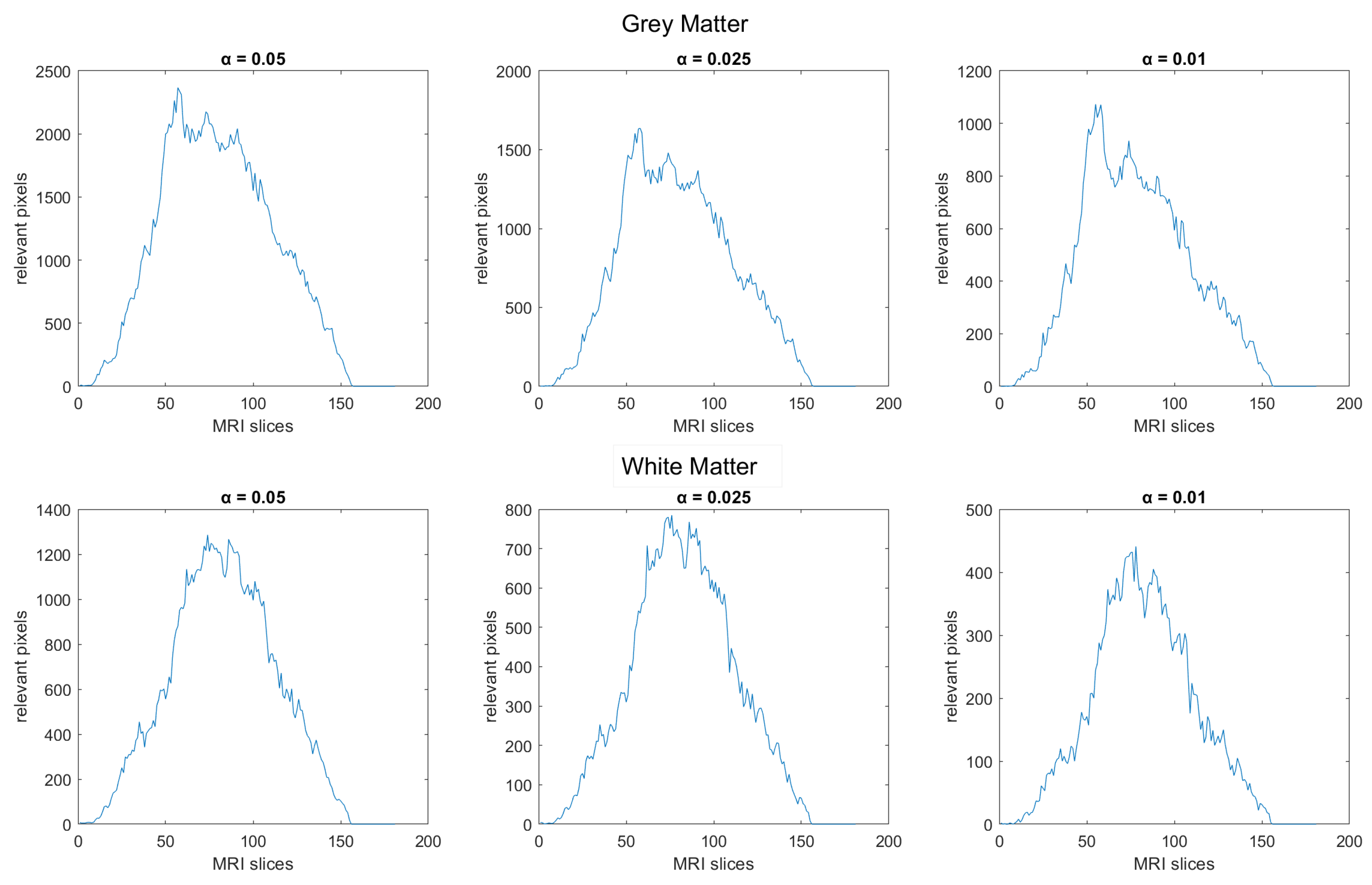
The permutation test was performed using the matrices and , for the and and subjects, respectively, to detect, pixel by pixel, where white matter had a significant decreasing difference among the two classes. The same test was performed on gray matter. In both of them, the tests’ outputs resulted in a two-p-valued 3D matrix. The significant pixels were computed by thresholding the output matrices in relation to the three standard values, i.e., , , and . The final distribution is plotted in Figure 4 with respect to the 181 sagittal MRI slices.
In the distribution of the two matters, we observed a high-density area that is common to all the thresholds, where we proceeded in selecting the MRI horizontal slices, so lying in the interval [56: 105] for the white matter, and in the interval [51: 110] for the gray matter. Only the significant pixels of these slices were considered in the next K-means clustering step. As one can observe in Figure 4, for different , the peak areas of the white matter are similar (but not equal) to those of the gray matter; for this reason, we properly chose the intervals of slices.
3.2. K-Means Clustering and Centroid Detection: Classes AD and NC
As input, the K-means clustering process had a sequence of 90 matrices containing white (resp. gray) values of the 40 and 50 subjects in the detected significant pixels belonging to the chosen slices’ intervals. Those matrices resulted in sizes of (resp. ), and we indicate them as , (resp. , ) for each subject and .
To speed up the process, since the two expected clusters were known, we set the matrices’ means of the classes and (resp. and ) as the starting centroids. Convergence was obtained after less than 10 iterations and led to two centroids that we indicated as and (resp. and ).
In order to estimate the difference in the computational time of theclustering process when acting on the significant pixels only, we also performed the K-means on the full-values matrices , (resp. , ). Table 1 shows the obtained computational times of illustrative runs of the K-means algorithm on an Intel(R) Core(TM) i7-4770 processor (speed: GHz) and 32 GB RAM.
Then, we tested the separability of the classes according to the detected centroids. Table 2 and Table 3 show the obtained results for the and classes. We underline that white matter clustering performed optimally, while gray matter clustering missed about of the subjects. A discussion on this phenomenon will follow in Section 4. A visual inspection of the computed subject-to-centroid distances showed that no outliers were present.
We point out that the K-means clustering process has been also performed varying both the considered distance measure, in particular using the Euclidean, Czekanowski, Chebyshev, and City Block distances, and the slices’ interval widths, always keeping the central highest significant pixels density areas. What is reported here is the optimal performance (not only in time but also in accuracy, according to the parameters’ choices and related to the Euclidean distance) among all the K-means instances. For the sake of completeness, we show in Figure 5 the confusion matrices of the K-means clustering related to the classes and , according to the four distances indicated above.
3.3. MCI-to-AD Predictions Based on Centroid Distances
The detected centroids and (resp. and ) were used in the final stage of this research to predict the subjects that showed an pattern similar to the patients diagnosed with . Now, we moved to the 101 MRI images (resp. ) for each and we selected the white (resp. gray) significant pixels in the same interval [56:105] (resp. [51:110]) considered for white (resp. gray) matter classification of the and subjects, obtaining the matrix (resp. ). In closing, the distances and (resp. and ) between each subject and the two centroids were calculated in order to proceed to the predictive classification.
Table 2 and Table 3 show the statistics of the performed classification task on white and gray matter, respectively.
Figure 6 shows the final intra-cluster distance distributions between subjects and the centroids of the corresponding clusters. Both the plots of the white and gray matter are provided. The values of the distributions’ means (W.c.d) and of the related standard deviations are reported in Table 2 and Table 3.
4. Discussion
This observational study pursued the aim of shedding light and gaining low computational cost on the predictive capability of white and gray matter decay in subjects, with respect to the same phenomenon in , related to normal aging, and , related to the Alzheimer’s disease course. As a matter of fact, different studies, even relying on the same type of data, produced quite different percentages of showing an pattern-like decay. The dataset we used contained MRI images from the public ADNI database of , , and subjects acquired in two scans separated by two years.
The results of our study can be summarized as follows:
- We have introduced the notion of significant pixels, i.e., the pixels of the MRI images where the white (resp. gray) matter decays in the considered two-year time span, significantly differ between and subjects. The number of significant pixels, in the brain slices where the phenomenon mostly appeared, according to the different values obtained after performing a permutation test on all the pixels of the images, i.e., , , and , was about 4%, 2%, and 1.5% of the totality of the white matter and slightly more, i.e., 6%, 4%, and 2.5%, of the totality of the gray matter. Such a small number of significant pixels is sufficient to discriminate between and , as reported in Table 2 and Table 3, using the K-means clustering technique. Not surprisingly, when considering the white matter, all the and subjects were correctly clustered, i.e., the white matter decay of subjects significantly differed from that of ones. On the other hand, when considering gray matter, the subjects were correctly classified, while 6 of the 40 subjects were assigned to the class, with a percentage of error of 15%. This can be ascribed to the fact that Alzheimer’s disease strongly impacts on the white matter first, and later leads to the decay of the gray matter.We also underline that, according to the wide and consolidated literature, the most involved areas of the brain affected by Alzheimer’s decay are the medial portion of the temporal lobe, where the hippocampus, amygdala, entoryl cortex, and parahippocampal cortex reside. These areas are located inside the selected slice intervals where most of the significant pixels were detected. As an example, Figure 7 shows the significant pixels of slice 58, where a peak in the white and gray matter occurred, with the involved brain areas highlighted.
- Moving to the -to- predictive capability of the K-means model restricted to significant pixels, again we found different percentages according to the considered white or gray matter in the considered two-year time span. As expected, analyzing the white matter a high percentage of , namely, (Table 2), showed an pattern-like decay, similar to what was detected in [16,17,18] on the same dataset. So, our result, with a time span of two years, was slightly below the results presented in [20], where after one year only 8 of 37 patients with converted to (22%), verifying the reduction in the regional glucose metabolic rate, a truthful signal of early-onset .This high percentage of pattern in could be attributed to the similarly located decay of white matter in the two classes of subjects, as reported in [43]. This study involved 23 , 15 , and 15 subjects that underwent diffusion tensor magnetic resonance imaging (DTI), an advanced MRI technique extremely sensitive to white matter alterations. The authors found that patients with had an increase in mean diffusivity in the limbic, interhemispheric, cortico-cortical, and corticospinal tracts and, similarly, patients with showed an increase in axial diffusivity only in tracts projecting to the frontal cortex and splenium of the corpus callosum.On the other hand, time passing caused a milder effect on the gray matter of subjects, whose analysis revealed only 29% of -to- cases (see Table 3),, in accordance with the more optimistic studies in the work of [8], obtained through using machine learning techniques on fMRI images.Table 2 and Table 3 report the obtained statistics on the classification performance of subjects, together with the related indexes. In Figure 6, the distributions of subjects’ distances within the clusters show smaller distances between the subjects and the related centroids when white matter is considered with respect to gray matter. This implies that the classification using white matter produces tighter clusters and, consequently, a stronger accuracy than gray matter. All the clusters show some borderline subjects that produce small local maxima while moving away from the centroids. However, the computation of the Dunn indexes showed the high reliability of the obtained clustering. Again, we underline that the small diameter of the cluster may also be due to the smaller variability in the age range of the subjects. However, this does not constitute an issue in the final results of the research.
- A crucial aspect of our research, related to point 1, concerns the possibility of using exclusively the significant pixels instead of the whole MRI images to significantly lower the computational costs (in time and resources) when performing statistics on the Alzheimer’s disease course. One can realize the benefits of shrinking the data size by about when nonlinear statistical analysis has to be performed or, even more, when machine learning predictive studies or feature detection are required. As a matter of fact, the step with the highest resource consumption in our research was the detection of the significant pixels, carried out by performing a permutation test on all the MRI image pixels, which lasted some days.Furthermore, lowering the computational costs of the classification task set the path for a real-time process to aid specialists’ examinations (and predictions) of the Alzheimer’s status and development.
A final comment, to stress a limitation to this study, relates to the very nature of the data: in the concept of , a wide range of different illnesses (pathological status) are included, such as depression, anxiety, sleep apnea, and also side effects of drugs; hence, for different reasons, not all subjects are destined to move into Alzheimer’s dementia. Actually, we did not know the specificity of each subject classification, and this may result in underestimating the real extent of the phenomenon. However, the only trustworthy bench mark of our and similar studies, is the follow-up of the subjects that will slip into Alzheimer’s disease and that, as quite rarely happens, will be the last word.
5. Conclusions
In this paper, we have defined the notion of significant pixels, i.e., a subset of pixels of an MRI image where most of the changes in white and gray matter are present during the AD degenerative process. After a first white and gray matter segmentation of and subjects obtained from the ADNI database, we performed a permutation test in order to obtain the positions where a significant difference between and appeared. In the literature, several ML approaches tried to detect and predict AD onset at an early stage from MRI scans, and used sophisticated models and features obtained from shape analysis and density variations that balanced accuracy with high computational time complexity. We stress that the obtained results, even from similar datasets, showed a wide range of variability. The use of significant pixels lowers the computational cost, preserving the information enclosed in the MRI dataset.
Concerning the prediction capability, first, the use of K-means on significant pixels was successfully tested to separate from subjects. Subsequently, the model was applied to the class and the coherence of the percentage predictions of -to- conversions with similar studies on the same dataset, i.e., [16,17,18] was verified. This could be of relevance in providing information about the subjects that changed from to together with the related time spans to further stress the accuracy of significant-pixel prediction on each subject. Unfortunately, in most of the databases used in the literature, including the ADNI database we relied on, those data are lacking or are not fully available.
So, our results on the ADNI population seem to indicate that significant pixels preserve the potential to detect with an AD-like pattern over a short span of time. Clinicians could have a real-time support diagnostic assessment in order to assist and carry out on their own patients in the natural course of the disease. Future research may benefit from the use of significant pixels, both for speeding up, by two orders of magnitude, the application of ML models on image datasets, and for restricting the prediction variability of the with -pattern-like subjects by pruning unnecessary and sometimes misleading information.
Author Contributions
Conceptualization, A.d.P., M.B. and A.F.; methodology, A.d.P.; software, M.B.; validation, M.B., A.d.P. and A.F.; formal analysis, M.B.; investigation, A.d.P., M.B. and A.F.; resources, A.d.P.; data curation, M.B.; writing—original draft preparation, A.d.P.; writing—review and editing, A.d.P., M.B. and A.F.; visualization, A.d.P. and M.B.; supervision, A.F.; project administration, A.F. All authors have read and agreed to the published version of the manuscript.
Funding
This research received no external funding.
Informed Consent Statement
Informed Consent Statements were collected by ADNI.
Data Availability Statement
All data are available on ADNI web site https://adni.loni.usc.edu/, accessed on 26 January 2024.
Acknowledgments
Data collection and sharing for this project was funded by the Alzheimer’s Disease Neuroimaging Initiative (ADNI) (National Institutes of Health Grant U01 AG024904) and DOD ADNI (Department of Defense award number W81XWH-12-2-0012). ADNI is funded by the National Institute on Aging, the National Institute of Biomedical Imaging and Bioengineering, and through generous contributions from the following: AbbVie, Alzheimer’s Association; Alzheimer’s Drug Discovery Foundation; Araclon Biotech; BioClinica, Inc.; Biogen; Bristol-Myers Squibb Company; CereSpir, Inc.; Cogstate; Eisai Inc.; Elan Pharmaceuticals, Inc.; Eli Lilly and Company; EuroImmun; F. Hoffmann-La Roche Ltd and its affiliated company Genentech, Inc.; Fujirebio; GE Healthcare; IXICO Ltd.; Janssen Alzheimer Immunotherapy Research & Development, LLC.; Johnson & Johnson Pharmaceutical Research & Development LLC.; Lumosity; Lundbeck; Merck & Co., Inc.; Meso Scale Diagnostics, LLC.; NeuroRx Research; Neurotrack Technologies; Novartis Pharmaceuticals Corporation; Pfizer Inc.; Piramal Imaging; Servier; Takeda Pharmaceutical Company; and Transition Therapeutics. The Canadian Institutes of Health Research is providing funds to support ADNI clinical sites in Canada. Private sector contributions are facilitated by the Foundation for the National Institutes of Health (www.fnih.org, accessed on 26 January 2024). The grantee organization is the Northern California Institute for Research and Education, and the study is coordinated by the Alzheimer’s Therapeutic Research Institute at the University of Southern California. ADNI data are disseminated by the Laboratory for Neuro Imaging at the University of Southern California.
Conflicts of Interest
The authors declare no conflict of interest.
References
- Gómez-Isla, T.; Price, J.L.; McKeel, D.W., Jr.; Morris, J.C.; Growdon, J.H.; Hyman, B.T. Profound Loss of Layer II Entorhinal Cortex Neurons Occurs in Very Mild Alzheimer’s Disease. J. Neurosci. 1996, 16, 4491–4500. [Google Scholar] [CrossRef]
- Laakso, M.P.; Soininen, H.; Partanen, K.; Lehtovirta, M.; Hallikainen, M.; Hänninen, T.; Helkala, E.-L.; Vainio, P.; Riekkinen, P.J. MRI of the Hippocampus in Alzheimer’s Disease: Sensitivity, Specificity, and Analysis of the Incorrectly Classified Subjects. Neurobiol. Aging 1998, 19, 23–31. [Google Scholar] [CrossRef]
- Arnold, S.E.; Hyman, B.T.; Flory, J.; Damasio, A.R.; Van Hoesen, G.W. The Topographical and Neuroanatomical Distribution of Neurofibrillary Tangles and Neuritic Plaques in the Cerebral Cortex of Patients with Alzheimer’s Disease. Cereb. Cortex 1991, 1, 103–116. [Google Scholar] [CrossRef] [PubMed]
- Oppenheim, G. The earliest signs of Alzheimer’s disease. J. Geriatr. Psychiatry Neurol. 1994, 7, 116–120. [Google Scholar] [CrossRef] [PubMed]
- Morris, J.C.; Cummings, J. Mild cognitive impairment (MCI) represents early-stage Alzheimer’s disease. J. Alzheimers Dis. 2005, 7, 235–239. [Google Scholar] [CrossRef] [PubMed]
- Hojjati, S.H.; Ebrahimzadeh, A.; Khazaee, A.; Babajani-Feremi, A. Predicting conversion from MCI to AD by integrating rs-fMRI and structural MRI. Comput. Biol. Med. 2018, 102, 30–39. [Google Scholar] [CrossRef] [PubMed]
- Feldman, H.; Scheltens, P.; Scarpini, E.; Hermann, N.; Mesenbrink, P.; Mancione, L.; Tekin, S.; Lane, R.; Ferris, S. Behavioral symptoms in mild cognitive impairment. Neurology 2004, 62, 1199–1201. [Google Scholar] [CrossRef]
- Hojjati, S.H.; Ebrahimzadeha, A.; Khazaee, A.; Babajani-Feremi, A. Predicting conversion from MCI to AD using resting-state fMRI, graph theoretical approach and SVM. J. Neurosci. Meth. 2017, 282, 69–80. [Google Scholar] [CrossRef] [PubMed]
- Ghafoori, S.; Shalbaf, A. Predicting conversion from MCI to AD by integration of rs-fMRI and clinical information using 3D-convolutional neural network. Int. J. Comput. Assist. Radiol. Surg. 2022, 17, 1245–1255. [Google Scholar] [CrossRef] [PubMed]
- Petersen, R.C.; Smith, G.E.; Waring, S.C.; Ivnik, R.J.; Tangalos, E.G.; Kokmen, E. Mild cognitive impairment: Ten years later. Arch. Neurol. 2009, 66, 1447–1455. [Google Scholar] [CrossRef]
- Rye, I.; Vik, A.; Kocinski, M.; Lundervold, A.; Lundervold, A. Predicting conversion to Alzheimer’s disease in individuals with Mild Cognitive Impairment using clinically transferable features. Sci. Rep. 2022, 12, 15566. [Google Scholar] [CrossRef]
- Adams, H.H.H.; de Bruijn, R.F.A.G.; Hofman, A.; Uitterlinden, A.G.; van Duijn, C.M.; Vernooij, M.W.; Koudstaal, P.J.; Ikram, M.A. Genetic risk of neurodegenerative diseases is associated with mild cognitive impairment and conversion to dementia. Alzheimers Dement. 2015, 11, 1277–1285. [Google Scholar] [CrossRef]
- Nicastro, N.; Malpetti, M.; Cope, T.E.; Bevan-Jones, W.R.; Mak, E.; Passamonti, L.; Rowe, J.B.; O’Brien, J.T. Cortical Complexity Analyses Their Cognitive Correlate in Alzheimer’s Disease Frontotemporal Dementia. J. Alzheimers Dis. 2020, 76, 331–340. [Google Scholar] [CrossRef] [PubMed]
- Rodríguez-Rodríguez, E.; Sánchez-Juan, P.; Vázquez-Higuera, J.L.; Mateo, I.; Pozueta, A.; Berciano, J.; Cervantes, S.; Alcolea, D.; Martínez-Lage, P.; Clarimón, J.; et al. Genetic risk score predicting accelerated progression from mild cognitive impairment to Alzheimer’s disease. J. Neural. Trans. 2013, 120, 807–812. [Google Scholar] [CrossRef] [PubMed]
- Afgin, A.E.; Massarwa, M.; Schechtman, E.; Israeli-Korn, S.D.; Strugatsky, R.; Abuful, A.; Farrer, L.A.; Friedl, R.P.; Inzelberget, R. High Prevalence of Mild Cognitive Impairment and Alzheimer’s Disease in Arabic Villages in Northern Israel: Impact of Gender and Education. J. Alzheimers Dis. 2012, 29, 431–439. [Google Scholar] [CrossRef] [PubMed]
- Davatzikos, C.; Bhatt, P.; Shaw, L.M.; Batmanghelich, K.N.; Trojanowski, J.Q. Prediction of MCI to AD conversion, via MRI, CSF biomarkers, and pattern classification. Neurobiol. Aging 2011, 32, 2322.e19–2322.e27. [Google Scholar] [CrossRef] [PubMed]
- Fan, Y.; Batmanghelich, N.; Clark, C.M.; Davatzikos, C. Spatial patterns of brain atrophy in MCI patients, identified via high-dimensional pattern classification, predict subsequent cognitive decline. NeuroImage 2008, 39, 1731–1743. [Google Scholar] [CrossRef] [PubMed]
- Misra, C.; Fan, Y.; Davatzikos, C. Baseline and longitudinal patterns of brain atrophy in MCI patients, and their use in prediction of short-term conversion to AD: Results from ADNI. NeuroImage 1999, 44, 1415–1422. [Google Scholar] [CrossRef] [PubMed]
- Moradi, E.; Pepe, A.; Gaser, C.; Huttunen, H.; Tohka, J. Machine learning framework for early MRI-based Alzheimer’s conversion prediction in MCI subjects. NeuroImage 2015, 104, 398–412. [Google Scholar] [CrossRef] [PubMed]
- Mosconi, L.; Perani, D.; Sorbi, S.; Herholz, K.; Nacmias, B.; Holthoff, V.; Salmon, E.; Baron, J.-C.; De Cristofaro, M.T.R.; Padovani, A.; et al. MCI conversion to dementia and the APOE genotype, Wolters Kluwer Health. Neurology 2004, 63, 2332–2340. [Google Scholar] [CrossRef]
- Lin, W.; Gao, Q.; Yuan, J.; Chen, Z.; Feng, C.; Chen, W.; Du, M.; Tong, T. Predicting Alzheimer’s disease conversion from mild cognitive impairment using an extreme learning machine-based grading method with multimodal data. Front. Aging Neurosci. 2020, 12, 77. [Google Scholar] [CrossRef]
- Liu, S.; Cao, Y.; Liu, J.; Ding, X.; Coyle, D. A novelty detection approach to effectively predict conversion from mild cognitive impairment to Alzheimer’s disease. Int. J. Mach. Learn. Cybern. 2023, 14, 213–228. [Google Scholar] [CrossRef]
- Alashwal, H.; El Halaby, M.; Crouse, J.J.; Abdalla, A.; Moustafa, A.A. The Application of Unsupervised Clustering Methods to Alzheimer’s Disease. Front. Comput. Neurosci. 2019, 13, 31. [Google Scholar] [CrossRef]
- Kishore, P.; Usha Kumari, C.; Kumar, M.N.V.S.S.; Pavani, T. Detection and analysis of Alzheimer’s disease using various machine learning algorithms. Mater. Today Proc. 2021, 45, 1502–1508. [Google Scholar] [CrossRef]
- Li, H.; Habes, M.; Wolk, D.A.; Fan, Y. A deep learning model for early prediction of Alzheimer’s disease dementia based on hippocampal magnetic resonance imaging data. Alzheimers Dement. 2019, 15, 1059–1070. [Google Scholar] [CrossRef]
- Nijana, V.; Rajendran, P.S. Alzheimer’s Disease Prediction with K-means Clustering and Reinforcement Learning Approach. In Proceedings of the 2023 International Conference on Distributed Computing and Electrical Circuits and Electronics (ICDCECE), Ballar, India, 29–30 April 2023; pp. 1–6. [Google Scholar]
- Gao, F.; Yoon, H.; Xu, Y.; Goradia, D.; Luo, J.; Wu, T.; Su, Y. Age-adjust neural network for improved MCI to AD conversion prediction. NeuroImage Clin. 2020, 27, 102290. [Google Scholar] [CrossRef] [PubMed]
- Jack, C.R., Jr.; Bernstein, M.A.; Fox, N.C.; Thompson, P.; Alexander, G.; Harvey, D.; Borowski, B.; Britson, P.J.; Whitwell, J.L.; Ward, C.; et al. The Alzheimer’s Disease Neuroimaging Initiative (ADNI): MRI methods. JMRI-J. Magn. Reson. Imaging 2008, 27, 685–691. [Google Scholar] [CrossRef] [PubMed]
- Tohka, J.; Minhas, S.; Khanum, A.; Alvi, A.; Riaz, F.; Khan, S.A.; Alsolami, F.; Khan, M.A. Early MCI-to-AD Conversion Prediction Using Future Value Forecasting of Multimodal Features. Comput. Intell. Neurosci. 2021, 2021, 6628036. [Google Scholar]
- Kaufman, A.S.; Lichtenberger, E. Assessing Adolescent and Adult Intelligence, 3rd ed.; Wiley: Hoboken, NJ, USA, 2006. [Google Scholar]
- Folstein, M.F.; Folstein, S.E.; McHugh, P.R. Mini-mental state. A practical method for grading the cognitive state of patients for the clinician. J. Psychiatr. Res. 1975, 12, 189–198. [Google Scholar] [CrossRef]
- Hughes, C.P.; Berg, L.; Danziger, W.L.; Coben, L.A.; Martin, R.L. A new clinical scale for the staging of dementia. Br. J. Psychiatry 1982, 140, 566–572. [Google Scholar] [CrossRef]
- Hachinski, V.C.; Iliff, L.D.; Zilhka, E.; Du Boulay, G.H.; McAllister, V.L.; Marshall, J.; Russell, R.W.R.; Symon, L. Cerebral blood flow in dementia. Arch. Neurol. 1975, 32, 632–637. [Google Scholar] [CrossRef] [PubMed]
- Sheikh, J.I.; Yesavage, J.A.; Brooks, J.O.; Friedman, L.; Gratzinger, P.; Hill, R.D.; Zadeik, A.; Crook, T. Proposed factor structure of the Geriatric Depression Scale. Int. Psychogeriatr. 1991, 3, 23–28. [Google Scholar] [CrossRef]
- ADNI. MRI Analysis. Available online: https://adni.loni.usc.edu/methods/mri-tool/mri-analysis/ (accessed on 20 March 2023).
- Whitfield-Gabrieli, S.; Nieto-Castanon, A. Conn: A functional connectivity toolbox for correlated and anticorrelated brain networks. Brain Connect. 2012, 2, 125–141. [Google Scholar] [CrossRef] [PubMed]
- Nieto-Castanon, A. Handbook of Functional Connectivity Magnetic Resonance Imaging Methods in CONN; Hilbert Press: Boston, MA, USA, 2020. [Google Scholar]
- Fonov, V.S.; Evans, A.C.; Botteron, K.; Almli, C.R.; McKinstry, R.C.; Collins, D.L.; Brain Development Cooperative Group. Unbiased average age-appropriate atlases for pediatric studies. NeuroImage 2011, 54, 313–327. [Google Scholar] [CrossRef] [PubMed]
- Ashburner, J.; Friston, K.J. Unified segmentation. NeuroImage 2005, 26, 839–851. [Google Scholar] [CrossRef] [PubMed]
- Moore, J.H. Bootstrapping, permutation testing and the method of surrogate data. Phys. Med. Biol. 1999, 44, L11. [Google Scholar] [CrossRef]
- Hartigan, J.A.; Wong, M.A. Algorithm AS 136: A K-Means Clustering Algorithm. J. R. Stat. Soc. Ser. C (Appl. Stat.) 1979, 28, 100–108. [Google Scholar] [CrossRef]
- Dunn, J.C. Well-Separated Clusters and Optimal Fuzzy Partitions. J. Cybern. 1974, 4, 95–104. [Google Scholar] [CrossRef]
- Agosta, F.; Pievani, M.; Sala, S.; Geroldi, C.; Galluzzi, S.; Frisoni, G.B.; Filippi, M. White Matter Damage in Alzheimer Disease and Its Relationship to Gray Matter Atrophy. Radiology 2011, 258, 853–863. [Google Scholar] [CrossRef]
Figure 1.
Block diagram of the study design. The data collected from the ADNI database first undergoes a pre-processing stage where white and gray matter are segmented. Then, a permutation test on the white and gray matter of and subjects allows significant pixels to be detected and to restrict the dataset accordingly. The involved classes are defined in Section 3 and Section 3.2. Finally, a ML model, K-means, is trained, tested, and employed to distinguish between normal aging and AD degeneration, as well as predict candidates exhibiting the MCI-to-AD pattern.

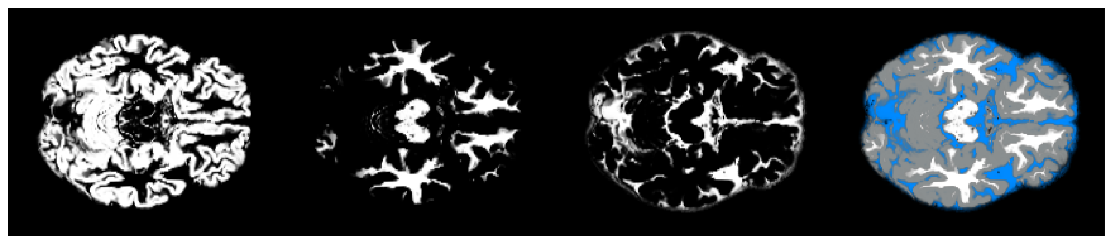
Figure 2.
The axial slice 58 view of gray matter, white matter, and fluid (from left to right) extracted from MRI data of an AD subject. The pixel classification is performed with the Matlab CONN toolbox.
Figure 2.
The axial slice 58 view of gray matter, white matter, and fluid (from left to right) extracted from MRI data of an AD subject. The pixel classification is performed with the Matlab CONN toolbox.

Figure 3.
From left to right, the axial slice 58 view of gray matter at , time acquisitions and their difference, highlighted in red. The data are from the MRI of an AD subject.
Figure 3.
From left to right, the axial slice 58 view of gray matter at , time acquisitions and their difference, highlighted in red. The data are from the MRI of an AD subject.

Figure 4.
Significant pixels’ distribution for the white and gray matter according to the three different thresholds.
Figure 4.
Significant pixels’ distribution for the white and gray matter according to the three different thresholds.

Figure 5.
The confusion matrices computed after the K-means clustering of the and classes with respect to the four (Euclidean, Czekanowski, Chebyshev, and City Block) distances (the first one outperforming the others). The distances led to convergence after 2, 8, 10, and 6 iterations, respectively.
Figure 5.
The confusion matrices computed after the K-means clustering of the and classes with respect to the four (Euclidean, Czekanowski, Chebyshev, and City Block) distances (the first one outperforming the others). The distances led to convergence after 2, 8, 10, and 6 iterations, respectively.

Figure 6.
Subject-to-centroid distance distributions inside each cluster.

Figure 7.
Slice 58 of an subject. (Left) white and gray matter locations. (Right) the significant pixels of the same slice and the brain areas in which they are located, divided according to Brodmann areas. The vast majority of significant pixels are located in the fusiform gyros, hyppocampus, amigdala, parahippocampal gyrus, and orbitofrontal lobe.


Table 1.
The computational time performance (in seconds) of illustrative runs of the K-means clustering algorithm on the full MRI images vs. the significant pixels only. The differences between white and gray matter, as well as between the full MRI images and the selected slice intervals, are also highlighted.
| Full MRI Images | Selected MRI Slice Intervals | |||
|---|---|---|---|---|
| All Pixels | Significant Pixels | All Pixels | Significant Pixels | |
| White matter | 29.362 s | 0.823 s | 18.403 s | 0.569 s |
| Gray matter | 70.584 s | 1.501 s | 19.462 s | 0.709 s |
Table 2.
Results of the clustering analysis of the subjects performed on the significant pixels only of the white matter segmentation. Cl.D.: cluster diameter; W.c.d.: within cluster distance, i.e., the mean of the distances from the subjects and the centroids of the class and the related standard deviation, i.e., Std. Dev.; DI: Dunn Index.
| Subjects | Cl.D. | W.c.d. | Std. Dev. | DI | |
|---|---|---|---|---|---|
| NC | 50 | 11,261.55 | 6313.38 | 662.79 | 0.56 |
| AD | 40 | 19,933.77 | 7236.79 | 1746.69 | 0.36 |
| MCI-to-AD | 37 | 20,832.19 | 8452.98 | 2677.15 | 0.40 |
| MCI | 64 | 14,954.89 | 7030.72 | 1271.85 | 0.47 |
Table 3.
Results of the clustering analysis of the subjects performed on the significant pixels only of the gray matter segmentation. Cl.D.: cluster diameter; W.c.d.: within cluster distance, i.e., the mean of the distances from the subjects and the centroids of the belonging class and the related standard deviation, i.e., Std. Dev.; DI: Dunn Index.
| Subjects | Cl.D. | W.c.d. | Std. Dev. | DI | |
|---|---|---|---|---|---|
| NC | 56 | 17,447.07 | 9581.68 | 1008.61 | 0.55 |
| AD | 34 | 24,415.07 | 11,426.67 | 1909.34 | 0.47 |
| MCI-to-AD | 29 | 24,291.55 | 12,768.19 | 2106.07 | 0.53 |
| MCI | 72 | 20,219.51 | 10,482.42 | 1360.34 | 0.52 |
Disclaimer/Publisher’s Note: The statements, opinions and data contained in all publications are solely those of the individual author(s) and contributor(s) and not of MDPI and/or the editor(s). MDPI and/or the editor(s) disclaim responsibility for any injury to people or property resulting from any ideas, methods, instructions or products referred to in the content. |
© 2024 by the authors. Licensee MDPI, Basel, Switzerland. This article is an open access article distributed under the terms and conditions of the Creative Commons Attribution (CC BY) license (https://creativecommons.org/licenses/by/4.0/).
Share and Cite
MDPI and ACS Style
Bellezza, M.; di Palma, A.; Frosini, A. Predicting Conversion from Mild Cognitive Impairment to Alzheimer’s Disease Using K-Means Clustering on MRI Data. Information 2024, 15, 96. https://doi.org/10.3390/info15020096
AMA Style
Bellezza M, di Palma A, Frosini A. Predicting Conversion from Mild Cognitive Impairment to Alzheimer’s Disease Using K-Means Clustering on MRI Data. Information. 2024; 15(2):96. https://doi.org/10.3390/info15020096
Chicago/Turabian StyleBellezza, Miranda, Azzurra di Palma, and Andrea Frosini. 2024. "Predicting Conversion from Mild Cognitive Impairment to Alzheimer’s Disease Using K-Means Clustering on MRI Data" Information 15, no. 2: 96. https://doi.org/10.3390/info15020096
Note that from the first issue of 2016, this journal uses article numbers instead of page numbers. See further details here.