An Empirical Study of Deep Learning-Based SS7 Attack Detection

Abstract

Signalling protocols are responsible for fundamental tasks such as initiating and terminating communication and identifying the state of the communication in telecommunication core networks. Signalling System No. 7 (SS7), Diameter, and GPRS Tunneling Protocol (GTP) are the main protocols used in 2G to 4G, while 5G uses standard Internet protocols for its signalling. Despite their distinct features, and especially their security guarantees, they are most vulnerable to attacks in roaming scenarios: the attacks that target the location update function call for subscribers who are located in a visiting network. The literature tells us that rule-based detection mechanisms are ineffective against such attacks, while the hope lies in deep learning (DL)-based solutions. In this paper, we provide a large-scale empirical study of state-of-the-art DL models, including eight supervised and five semi-supervised, to detect attacks in the roaming scenario. Our experiments use a real-world dataset and a simulated dataset for SS7, and they can be straightforwardly carried out for other signalling protocols upon the availability of corresponding datasets. The results show that semi-supervised DL models generally outperform supervised ones since they leverage both labeled and unlabeled data for training. Nevertheless, the ensemble-based supervised model NODE outperforms others in its category and some in the semi-supervised category. Among all, the semi-supervised model PReNet performs the best regarding the Recall and F1 metrics when all unlabeled data are used for training, and it is also the most stable one. Our experiment also shows that the performances of different semi-supervised models could differ a lot regarding the size of used unlabeled data in training.

1. Introduction

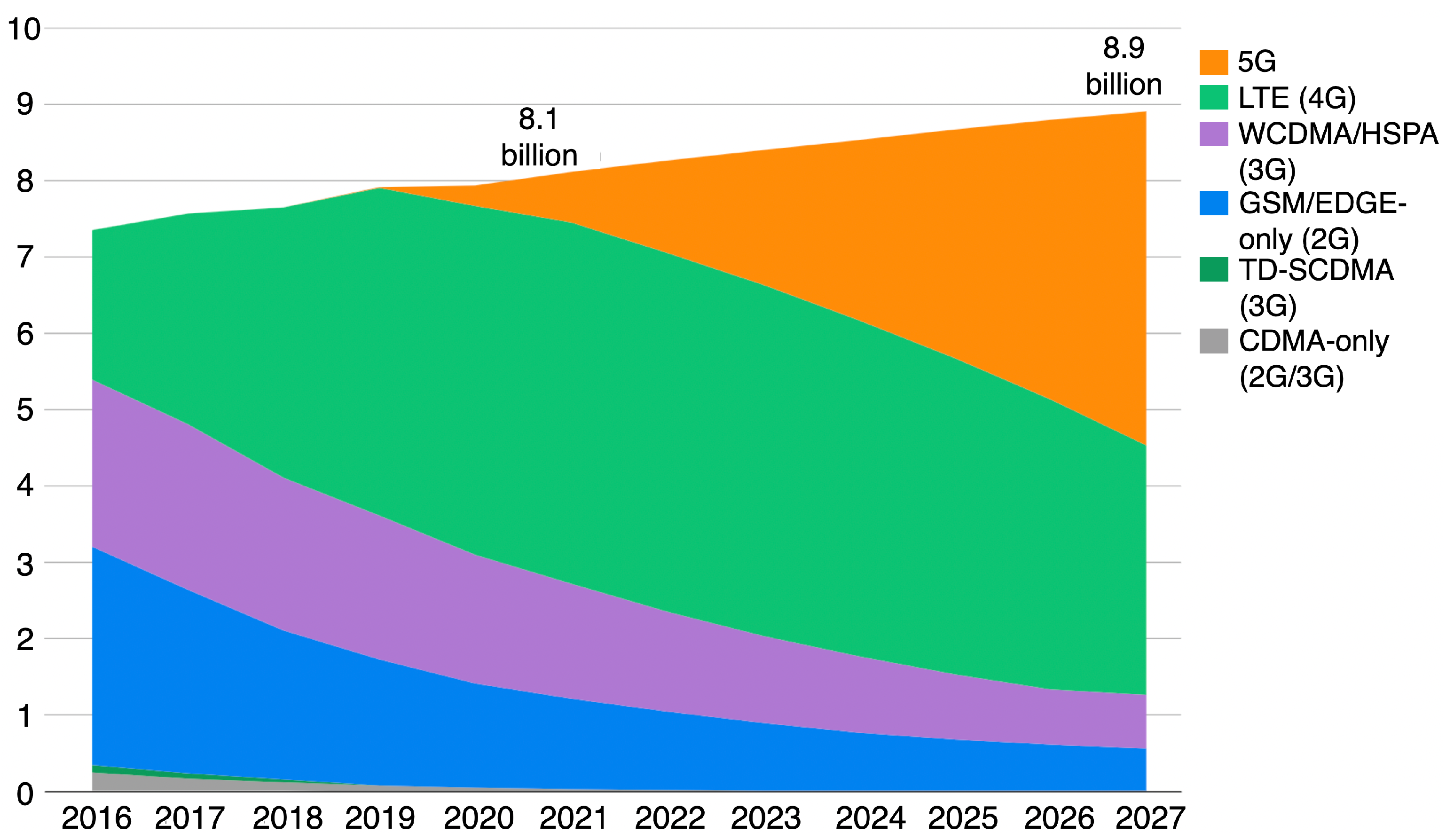
Since their initial arrival in the late 1970s, mobile networks have evolved fast and are playing an ever-increasing role in our lives. The first generation (i.e., 1G) relies on analogy technology and only allows voice calls to be made. It suffers from serious reliability and signal interference issues. At the beginning of the 1990s, the second generation (i.e., 2G) was introduced based on digital signalling technology. Besides voice calls, it allows users to send Short Message Service (SMS) and Multimedia Messaging Service (MMS) messages, although at low speeds. In 2000, the third generation (i.e., 3G) was introduced to allow users to make video calls, surf the web, share files, play online games and even watch TV online. Just before 2010, the fourth generation (i.e., 4G) was introduced while a lot of new technologies were developed in between (e.g., 3.5G and so on). In comparison to 3G, 4G improves the quality of services, latency reduction and supports many new services such as broadband, mobile TV and HDTV. Since 2019, the fifth generation (5G) has started to be deployed. Its key features include Enhanced Mobile Broadband (eMBB), Ultra Reliable Low Latency Communications (URLLC), and Massive Machine Type Communications (mMTC). Furthermore, 5G adopts the concept of SBA (Service-Based Architecture) for its core and enhances its security. In comparison to the previous generations, 5G heavily relies on standard Internet protocols, such as TCP/IP and HTTP; while 5G is gradually being deployed and 4G has covered most of the population, the earlier generations (2G and 3G) are still in place as illustrated in Figure 1. In many regions, only lower-generation networks are supported, and the service will be downgraded from 5G to lower generations in certain circumstances.

In telecommunication, signalling protocols are used for organizing signalling exchanges among communication endpoints and switching systems. We can say that such protocols are the foundation of managing the mobile networks. Signalling Security No. 7 (SS7) is the signalling protocol used in 2G and 3G networks. In 4G, particularly long-term evolution (LTE), signalling mainly relies on the Diameter protocol, which was originally designed by IETF for Authentication, Authorization, and Accounting (AAA). In 5G, signalling messages are transmitted through standard HTTP protocols [1] and they form part of the transactions in the Control Plane. Due to their key role in running mobile networks, the security of signalling protocols has received more and more attention. Notably, in 2018, the European Union Agency for Cybersecurity (ENISA) published a report on the security issues in these signalling protocols and highlighted that too little research had been conducted on the topic [2]. Unfortunately, as we have shown in Section 2.2, the situation has not changed much, and there are very few papers on this topic up to today.

The co-existence of various generations of technologies raises serious cybersecurity concerns, especially the issues regarding signalling protocols. It is common that an attack will exploit the vulnerabilities in SS7 and launch downgrade attacks to bypass the security mechanisms in 4G and 5G [3]. For instance, in [4], it is shown that vulnerabilities in SS7 protocol can be exploited to mount attacks in roaming and interconnection environments, perform location tracking, call/SMS interception, fraud, DoS, spoofing and threaten the security of 5G core networks. As such, studying the security of SS7 is still an interesting topic, even though 3G has been a legacy technology for many years. On the other hand, recent advances in this domain have shown that the use of machine-learning-based approaches can provide efficient results in terms of detecting the SS7 attacks [5,6]. Using deep learning-based solutions is more efficient than other machine-learning-based solutions, particularly for the detection of SMS interception attacks. Therefore, our main motivation is to evaluate the performance of popular deep learning-based models on anomaly detection for distinguishing SS7 attacks from normal events.

1.1. Our Contributions

Artificial Intelligence (AI) or Machine Learning (ML) technologies have been widely used for cybersecurity purposes such as anomaly detection and fraud detection, and recent advancements with Deep Learning (DL) and Large Language Models (LLMs) are accelerating the landing of these technologies. In the telecommunication security domain, due to the scarcity of datasets, only a few works exist, e.g., [7,8]. The potential of AI/ML has been underdeveloped.

In this paper, we aim to provide a systematic study of state-of-the-art (SOTA) DL models, including both supervised and semi-supervised approaches. To make our analysis meaningful and realistic for the target scenario, we leverage both a proprietary dataset and a simulated dataset. The proprietary dataset is constructed from the network traffic of a Telecom service provider in Luxembourg, and some labeled data examples have been generated by domain experts as the ground truth. Regarding DL-based attack detection solutions, it is not always clear which metrics should be used to evaluate the performances (e.g., a DoS attack and an APT attack). To clarify this issue in our scenario, we provide a brief analysis of four metrics, namely accuracy, precision, recall and F1. We show that recall and F1 are the most valuable metrics, while accuracy and precision are less useful and could also be misleading.

Our experimental results bring several insights into applying ML to attack detection in our scenario. One is that semi-supervised models are generally better than the supervised ones due to the addition of a large amount of unlabeled data. In particular, the PReNet [9] performs the best on both datasets with respect to both recall and F1, when all unlabeled data are used for training. Furthermore, its standard derivation is much smaller than other models, which means that its performance is consistent and stable. The second is that the ensemble method, namely the NODE [10] model, performs the best among the supervised models and also outperforms some semi-supervised models. This coincides with the fact that ensemble methods usually have better performances in ML-based solutions such as recommender systems. It is worth noting that both PReNet and NODE outperform the CNN-based method from [8] regarding almost all the metrics. Lastly, regarding the relation between performance and the size of unlabeled data (used for training), DevNet quickly reaches its best performance regarding all metrics. PReNet and SSL_CNN exhibit a consistent trend in performance increase when more unlabeled data are used for training, while PReNet performs far better. The Deep SAD has more ad hoc behaviour and worse performance. In practice, whether DevNet or PReNet should be used will need further experiments with larger datasets.

1.2. Organisation

The paper is organized as follows. Section 2 provides an overview of the main functions of the SS7 protocol and related work. Section 3 covers the methodology of the empirical study and experimental design. Section 4 analyzes the experimental results. Finally, Section 5 concludes the work.

2. Preliminary and Related Work

This section introduces the SS7 protocol in detail and summarizes the related work on SS7 security.

2.1. SS7 Protocol Overview

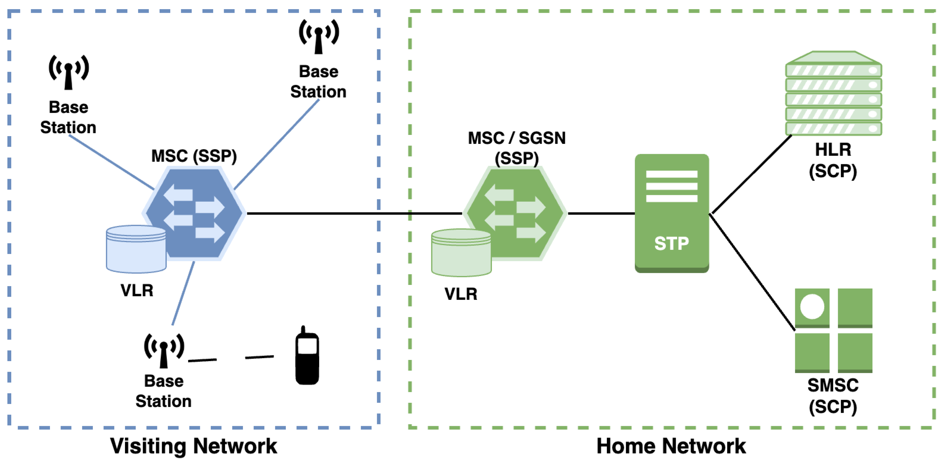
SS7 is the signalling protocol that is used by 2G (GSM) and 3G (UMTS/CDMA) telecommunication technologies. Over the years, SS7 has been upgraded with new functionalities such as the use of the Signalling Transport (SIGTRAN) protocol in order to achieve interoperability with other communication protocols (i.e., IP and GPRS). The general architecture of SS7/SIGTRAN networks contains three important nodes as illustrated in Figure 2:

• Service Switching Points (SSPs): This node is the interface of the SS7 network to the outside world such as the Mobile Switching Center (MSC) or Serving GPRS Support Node (SGSN) in the core network. MSC is used to transfer voice and data between user equipment and core network entities. SGSN, which is introduced with 3G technology, is responsible for handling incoming/outgoing geolocation-related packets in the core network.
• Signal Transfer Points (STPs): This node operates as a router between SSPs and SCPs in the SS7 network.
• Service Control Points (SCPs): This node operates as a gateway between STPs and operator’s databases (i.e., Home Location Register—HLR, Visitor Location Register—VLR, Short Message Service Center—SMSC, etc.) HLR is the main subscriber database that stores all the information regarding subscribers. VLRs are temporary databases attached to MSCs to store the information related to (visiting) subscribers connected to MSCs. Hence, the communication overhead between MSCs and HLR is reduced. SMSC is used for executing all SMS-related tasks such as receiving, storing, and forwarding SMS messages, etc.

SS7 core network elements are not limited to the ones presented in Figure 2. There exist some other entities such as Media Gateway (MGW) to enable Voice over IP, Session Border Control (SBC) to provide security against attacks, and Gateway GPRS Support Node (GGSN) to establish communication between an SGSN and external data networks (i.e., by converting incoming traffic into IP-based traffic). However, we focus on a specific type of SS7 attack in this study, and the SS7 core network elements explained in this section are selected accordingly.

2.2. Related Work on SS7 Security

The SS7 protocol is vulnerable to various security attacks such as the disclosure of IMSI (International Mobile Subscriber Identity), location of the subscriber, disruption of subscriber’s availability, interception of calls and SMS messages, etc. [5]. The main reason behind those attacks is that SS7 does not have a proper security mechanism to protect call flows (the callflow is the process of handling calls (voice or data) or information exchange in the telecommunication network) [11]. Each call flow contains a sequence of messages to transfer the necessary information between the core network entities and subscribers. Those messages are categorized into three groups based on the location (home network or visiting network) that they initiated as introduced in GSMA IR.82 [12]. Categories of SS7 messages are as follows:

• Category 1 (Cat. 1): The message originator and receiver are located in the home network.
• Category 2 (Cat. 2): The message originator is in the home network and the receiver is in the visiting network.
• Category 3 (Cat. 3): The message originator is in the visiting network and the receiver is in the home network.

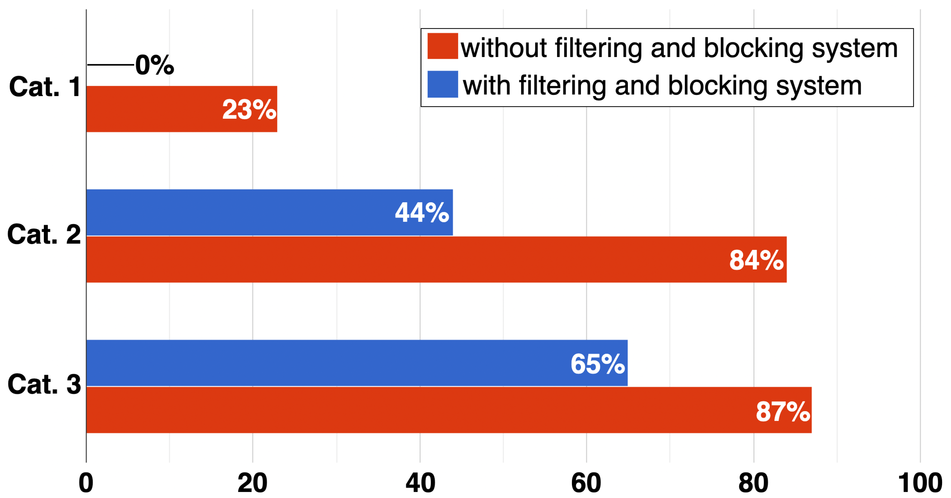
From the security perspective, this categorization plays a critical role in terms of the selection of the appropriate defence mechanism. The report of Positive Technologies on SS7 security vulnerabilities [11] underlines the effectiveness of using rule-based detection mechanisms (i.e., filtering and blocking mechanisms) against attacks for each message category (Figure 3). In more detail, using filtering and blocking mechanisms can eliminate all attacks that target Cat. 1 messages, which have a 23% success rate when there is no defence mechanism in place. On the other hand, attacks that target Cat 2. and Cat 3 messages have higher success rates (84% and 87%, respectively) if no defence mechanism is applied for those message categories. Using filtering and blocking systems can eliminate almost half (44%) of the attacks for Cat. 2 messages; however, they can only filter out 25% of the attacks targeting Cat. 3 messages. This is because the originating node in Cat. 3 messages is not located in the home network (i.e., roaming partners of the service provider) and defence mechanisms located in the home network may not be effective in terms of obtaining information about the nodes in other networks. For instance, such mechanisms may mistakenly block some nodes in the other networks, and hence the subscribers connected to those nodes, because of the insufficient information about those nodes. To this end, for the attacks that target Cat. 3 messages, we need more powerful approaches than rule-based ones. One particular solution is to employ machine learning (ML)-based solutions to discriminate anomalies in Cat. 3 messages, as in [5].

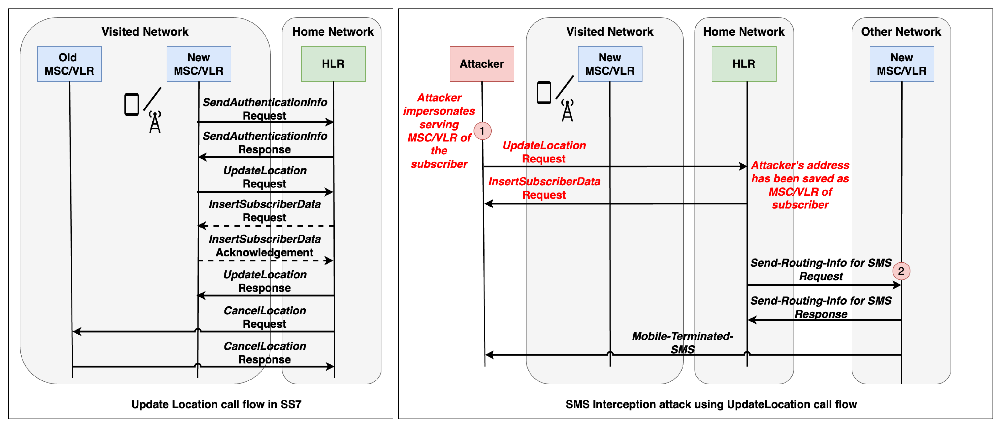
Considering the attacks that target Cat. 3 messages, the SMS interception attack using Update Location (UL) call flow is the most critical one. In that scenario, the attacker uses the International Mobile Subscriber Identifier (IMSI) number of any subscriber in the visiting network to obtain control of all incoming/outgoing SMS messages of that subscriber. If the attack is successful, the attacker is not only able to read or manipulate the SMS messages but also, it is possible to deploy additional attacks to amplify the damage such as using information in SMS messages to recieve access to third-party applications (i.e., online banking applications, e-mail systems, social network accounts, etc.). Figure 4 illustrates the legitimate Update Location call flow (left box) and SMS interception attack using Update Location call flow (right box). In the legitimate UL scenario, when a subscriber moves from one location to another, the location information can be updated in the home network depending on the coverage area of MSC(s)/VLR(s). Therefore, if needed, the subscriber information is removed from the old MSC/VLR and it is recorded in the new one. However, for the attack UL scenario, the attacker impersonates itself as the legitimate MSC/VLR and initiates the Update Location call flow. As a result of this attack, the new location is different than the original location and in general, this fake location cannot be a reasonable location when compared with the last update location call flow of the same subscriber. Hence, such kind of attacks are considered anomalies in the UL call flows and they can be detected via using ML-based solutions as presented in [5,6,7,8]. In this work, our main motivation is to analyze efficient ML-based solutions for the detection of anomalies in Update Location call flow.

2.3. Other Further Related Work

Anomaly detection is a challenging task for ML applications that have been studied over the years in various application domains such as the network anomaly detection (detection of Distributed Denial of Service—DDoS attacks) [13,14,15,16,17], video/image anomaly detection [18,19,20], telecommunication signalling anomaly detection [5,7,8,21], etc. ML-based solutions that are applied to the anomaly detection tasks are also categorized based on the ML paradigm, namely the supervised, unsupervised and semi-supervised learning techniques. Among those techniques, the supervised learning-based solutions are expected to be the most efficient in terms of detecting anomalies if the underlying ML model is well-trained. However, due to the very nature of the problem, in the anomaly detection task, we need to handle a large dataset with very few labeled instances. Therefore, it is generally unlikely to train an effective ML model except for some special cases such as detecting anomalies due to some disease in medical images [18]. On the other hand, with the surge in deep learning technologies, unsupervised approaches such as auto-encoder neural networks have increased their popularity for their use in anomaly detection tasks [13,20]. The idea is therefore to re-generate the input using an auto-encoder model and then calculate the re-construction error using the difference between the input and output. Then, if the error is higher than a certain threshold, it is called anomaly for a given task. However, such kind of an assumption may fail due to the ML task is reduced into a simple distance-based threshold check problem and accordingly, the false-positive (a normal condition predicted as an anomaly) rate may increase [7].

On the other hand, recent studies [8,14] show that convolutional neural networks (CNNs) are an important ML approach for the detection of anomalies since they also reduce the false positive rate. Particularly, the study in [8] adopts a multi-class semi-supervised learning approach based on CNN in [22] for the detection of anomalies due to the attacks targeting SS7 Update Location call flows. Our goal in this study is to extend the work in [8] by empirically comparing this work with various recent and popular supervised and semi-supervised learning models.

3. Our Empirical Study

Figure 5 gives an overview of this study. Given the labeled and unlabeled data, the first step is to execute feature selection. This step serves to eliminate less meaningful features, largely reducing the run time complexity. Subsequently, the second step encompasses the training of a DL-based detection model. If a supervised model is selected, only labeled data will be used for training. Otherwise, unlabeled data are added to the training set for semi-supervised training. Lastly, the performance of different models will be compared based on different evaluation metrics.

3.1. Problem Formulation

The detection task is treated as a binary classification problem. Note that the detection task can be treated as a multi-class classification problem for identifying specific classes of attacks, only if the attack information is present in the data. However, the datasets at hand only have binary labels. Let $f\left(\mathbf{x},y\right)$ be a binary classifier that maps the input $\mathbf{x}$ into its corresponding label y (0: normal, 1: abnormal). In this context, $\mathbf{x}$ represents the feature vector containing a set of features, while y denotes the ground truth label associated with $\mathbf{x}$. Specifically, the features can be divided into two groups: categorical and numerical. Categorical features are discrete values from a predefined set of categories. For example, the transmitted update location messages are sent by HLR or SGSN. Numerical features are continuous values that represent quantitative measurements or counts, e.g., the number of unique countries visited in the last 10 min.

3.2. Datasets

One real-world and one simulated dataset are used in this study.

Real-world dataset: Provided by a Telecom service provider in Luxembourg, this dataset consists of the real-world SS7 traffic collected from the core network. The dataset contains 17,603 unlabeled records and 62 labeled (40 normal and 22 attack) instances. For the labeled dataset, all the attack instances are SMS interception attacks that use update location events. For the unlabeled dataset, we can consider that most of the instances are normal. Since the service provider has a filtering-based detection mechanism against attacks that target Cat. 1 and Cat. 2 messages, we can consider that the unlabeled dataset does not contain any attacks that target those categories. However, we do not have enough information regarding the attacks targeting Cat. 3 messages. Each dataset instance is represented with 43 features, which are categorized into four groups: (i) the current updateLocation events (Group 1), (ii) historical updateLocation events of a subscriber (Group 2) in last m minutes, (iii) last two updateLocation of the same IMSI (Group 3) in last m minutes, and (iv) historical events of the same Global Title (GT) in last m minutes (Group 4). Please refer to Appendix A for detailed explanations of features.

Simulated dataset: This dataset is created by the JSS7 attack simulator [23]. We run our experiments for 20 subscribers. The simulator generates 66,969 procedures, and 183 of them are attack procedures based on location tracking with ProvideSubscriberInfo, AnyTimeInterrogation events and SMS interception attacks using update location events. However, ProvideSubscriberInfo and AnyTimeInterrogation events are not related to Cat. 3 messages. Therefore, we have only considered SMS interception attacks which contain 4642 update location events of subscribers. Additionally, the JSS7 attack simulator deploys attacks for only one subscriber in the network, which is called the VIP subscriber. The traffic generated for the rest of the subscribers does not contain any attack and this traffic can be considered normal traffic. Therefore, we divided the records dataset into 85 labeled (as 57 normal and 28 attack) instances coming from the VIP subscriber and 4557 unlabeled records coming from normal subscribers. Later, we use the same features as the real-world dataset to extract simulated records.

3.3. Selected Models

Eight supervised and five semi-supervised models are implemented to train the binary classifier for detecting attacks. Those supervised models only use labeled data for training, while semi-supervised ones use both labeled and unlabeled data for training.

Supervised models:

• AutoInt [24]: The automatic feature interaction learning (AutoInt) model learns the high-order feature interactions of input features based on the self-attention mechanism [25]. AutoInt maps the sparse input features into low-dimensional representations through an embedding layer and an interacting layer which utilizes the multi-head self-attention.
• CategoryEmbedding [26]: This model is a simple feedforward neural network (FNN) with embedding layers for categorical features.
• SL_CNN [8]: This model is a simple convolutional neural network (CNN) with three convolutional layers. This model is the supervised version of the SSL_CNN model which will be described later.
• FT-Transformer [27]: Introduced by Yury et al., the FT Transformer (feature tokenizer + Transformer) is adapted from the Transformer [25] architecture for the tabular domain. FT-Transformer first converts all (categorical and numerical) input features into vector embeddings through a feature tokenizer. Second, these embeddings are processed by a stack of Transformer layers to obtain the final representation. FT-Transormer and AutoInt share a similar methodology.
• GATE [28]: The Gated Additive Tree Ensemble (GATE) model uses a gating mechanism, inspired by the gated recurrent unit (GRU) [29] in recurrent neural networks (RNN). GATE consists of three major modules in its architecture. First, the gated feature learning units (GFLUs) module receives all input features and learns the feature representation. Second, the differentiable non-linear decision trees (DNDTs) module takes these representations as input and builds the map between input and output. Finally, the ensembling multiple trees module generates the final result using the predictions from DNDTs based on the ensembling learning.
• NODE [10]: Similar to GATE, the Neural Oblivious Decision Ensembles (NODE) model uses ensembles of decision trees. Each hidden layer of NODE includes an ensemble of decision trees.
• TabNet [30]: Proposed by Arik and Pfister, TabNet uses sequential attention to determine the best feature at each decision step. Specifically, TabNet begins with applying a feature Transformer to capture interactions between features.
• TabTransformer [31]: Built on Transformer [25], TabTransformer is designed specifically for tabular data. Categorical features are fed into a sequence of multi-head attention-based Transformer layers to generate embeddings. These embeddings are later concatenated along with numerical features to form the vector representation. Finally, TabTransformer uses the multi-layer perception (MLP) with the vectors as input to produce predictions.

Semi-supervised models:

• DAE [26]: Denoising autoencoders (DAEs) are a type of unsupervised learning model that is commonly used for data denoising [32]. The key idea is to corrupt the input data with noise and train the autoencoder to reconstruct the original data (the reconstruction process is known as denoising).
• Deep SAD [33]: Based on the unsupervised deep support vector data description (SVDD) [34], the deep semi-supervised anomaly detection (SAD) generalizes the applicable scenario to semi-supervised anomaly detection setting. Instead of simply using unlabeled samples, Deep SAD additionally uses labeled samples for training. Specifically, Deep SAD integrates the loss on both unlabeled and labeled samples to design the objective function.
• DevNet [35]: The deviation network (DevNet) mainly contains an anomaly-scoring network and a reference score generator. The anomaly-scoring network simply uses the MLP network and produces anomaly scores for all samples (both labeled and unlabeled). The reference score generator is used to generate another anomaly score which is determined by a Gaussian prior probability on normal samples. Specifically, DevNet is equipped with a deviation loss function to combine the outputs from the scoring network and score generator. Note that all unlabeled samples are treated as normal inputs to the anomaly scoring network.
• PReNet [9]: The main idea of the Pairwise Relation prediction Network (PReNet) is to learn the pairwise relation of any two randomly selected samples. PReNet consists of two main modules: anomaly informed random instance pairing and pair-wise relation-based anomaly score learning. The first module generates a large set of instance pairs, including anomaly–anomaly pairs, anomaly–unlabeled pairs, and unlabeled–unlabeled pairs. Labels are given to each instance pair based on the pair type. By doing so, PReNet has a large labeled training set for the second module. The pair-wise relation-based anomaly score learning module uses a two-stream anomaly scoring network to learn linear pairwise relation features and anomaly scores.
• SSL_CNN [8]: Adapted from [22], the SSL_CNN model utilizes a simple CNN model for semi-supervised learning. In the pre-training step, unlabeled samples are fed into the CNN to tune its parameters. In the re-training step, these parameters are transferred to a new CNN which combines the first CNN and three dense layers, also called the fully connected layers. This new CNN is fine-tuned with labeled samples.

4. Experiments

All experiments are conducted on a high-performance computer cluster and each cluster node runs a 2.20 GHz Intel Xeon Silver 4210 CPU (Intel Corporation, Santa Clara, CA, USA) with an NVIDIA Tesla V100-PCIE-32 GB GPU (Nvidia Corporation, Santa Clara, CA, USA). All approaches are implemented using the PyTorch 1.13.0 framework.

4.1. Experimental Setup

4.1.1. Feature Selection

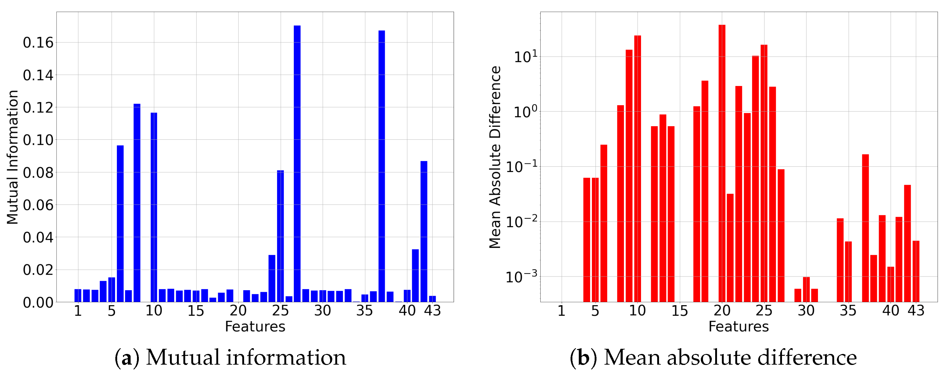
We observe that some features in the real-world dataset have the same value and hence, the same variance value for both the attack and normal subscriber records. These features have no or little effect on the detection rate. To this end, we employ mutual information (MI) (Figure 6a) to investigate the correlation between features and corresponding labels and mean absolute difference (MAD) (Figure 6b) to analyze the features concerning their distance to the average mean. Consequently, 31 features are selected for experiments.

4.1.2. Model Training

For supervised models, only labeled data are used. For semi-supervised models, both labeled and unlabeled data are used. The relevant data are randomly split into training and test (17 instances) sets for training and testing, respectively. Each model is trained for 200 epochs and the best performance is saved when it has the minimum loss on the test set. Detailed parameter settings are listed in Appendix B.

4.1.3. Evaluation

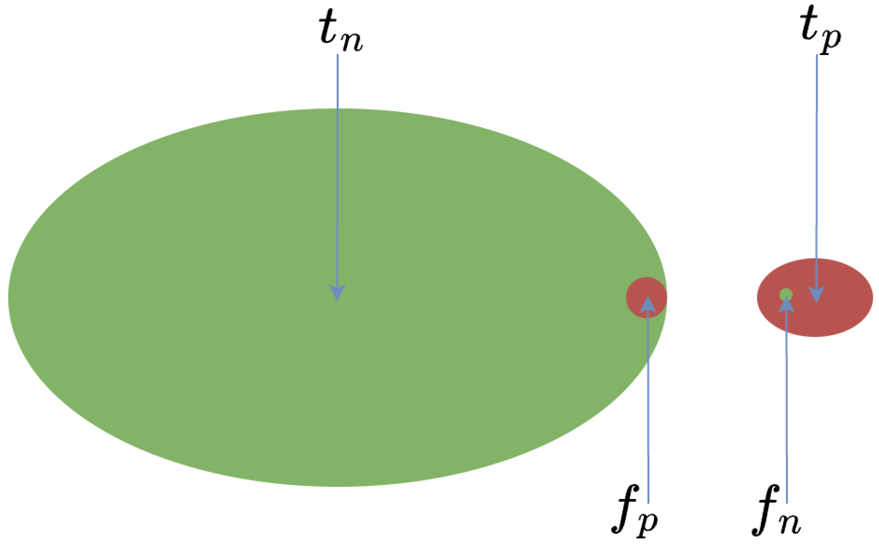
Four widely used metrics are used to quantify the model performance. Accuracy is defined as $\frac{tp+tn}{tp+fp+tn+fn}$. Precision is defined as $\frac{tp}{tp+fp}$. Recall is defined as $\frac{tp}{tp+fn}$. F1 is defined as $\frac{2\ast tp}{2\ast tp+fp+fn}$. The variables $tp,tn,fp,fn$ are defined as follows.

• True positive (tp): a positive (abnormal) instance is classified as positive.
• False positive (fp): a negative (normal) instance is classified as positive.
• True negative (tn): a negative instance is classified as negative.
• False negative (fn): a positive instance is classified as negative.

In our scenario, where an attacker tries to attack the signalling protocol in order to recieve privileged access, the proposition of the positive instances among the total number of instances is usually a very small number. This is similar to many other scenarios, where attackers aim at very specific objectives while being cautious to avoid detection. However, we note that for certain types of attacks, such as DDoS, the majority of the traffic will be positive due to the purpose of the attack. When deployed in practice, the true or false positive instances will usually analysed by human experts or other security mechanisms before actions are taken, depending on whether “real-time” is a required feature. This gives us two insights. One is that $fn$ should be minimised. If this variable is big, it will mean that attacks will pass without being detected. This leads to our argument that recall should be the most important metric in our evaluation. The other is that $fp$ is not a big issue as long as it remains relatively small so that it will neither cause a large burden nor disrupt the underlying service seriously. This leads to our argument that precision is the least important metric for our evaluation.

When the number of positive instances is much larger than the number of negative instances, the accuracy metric will be dominated by $tn$ as well as the ratio of $\frac{tn}{fp}$. As shown in Figure 7, when $\frac{tn}{fp}$ is big, then $tn$ will dominate the metric. Even if $fn$ becomes very big in comparison to $tp$, the impact on the accuracy will be slight. This implies that accuracy does not really give a good indication of how useful an ML model will be in our scenario. In contrast, F1 is very useful because a higher value will imply that the ratio between $fp$ (or $fn$) and $tp$ is lower. This is desirable in our scenario.

4.2. Results

Each experiment is repeated 100 times with different train-test split to report the statistical results (e.g., minimum, maximum, average, standard deviation).

4.2.1. Comparison among Models with All Unlabeled Data Used for Training

In this section, we report the comparison of all detection models on the simulated and real-world datasets.

Table 1. Comparison results (average ± standard deviation %) of 13 supervised (top) and semi-supervised (bottom) models on the real-world dataset. The best results are in bold. For all metrics, the higher, the better.

Model	Accuracy	Precision	Recall	F1
AutoInt	93.26 ± 10.74	95.39 ± 11.68	88.97 ± 16.68	90.89 ± 13.49
CategoryEmbedding	88.67 ± 10.97	86.51 ± 18.08	81.77 ± 18.97	82.86 ± 16.92
FT-Transformer	89.99 ± 11.22	92.41 ± 14.35	81.67 ± 22.23	84.26 ± 17.81
GATE	86.14 ± 10.96	91.39 ± 14.46	69.57 ± 22.97	76.29 ± 18.43
NODE	93.35 ± 5.68	97.96 ± 6.55	83.45 ± 15.28	89.01 ± 11.14
SL_CNN	80.19 ± 9.41	78.30 ± 19.03	66.66 ± 22.73	68.42 ± 16.03
TabNet	86.58 ± 13.39	89.35 ± 19.81	74.55 ± 23.33	78.70 ± 20.00
TabTransformer	84.45 ± 9.35	89.03 ± 14.95	65.07 ± 22.25	72.64 ± 18.60
DAE	71.03 ± 23.41	73.49 ± 27.27	76.95 ± 26.16	67.05 ± 20.79
Deep SAD	74.33 ± 9.06	60.17 ± 15.94	81.24 ± 17.47	67.55 ± 13.63
DevNet	91.53 ± 6.93	88.53 ± 12.04	86.98 ± 16.68	86.53 ± 12.10
PReNet	93.18 ± 5.62	86.25 ± 11.47	97.28 ± 8.02	90.93 ± 8.16
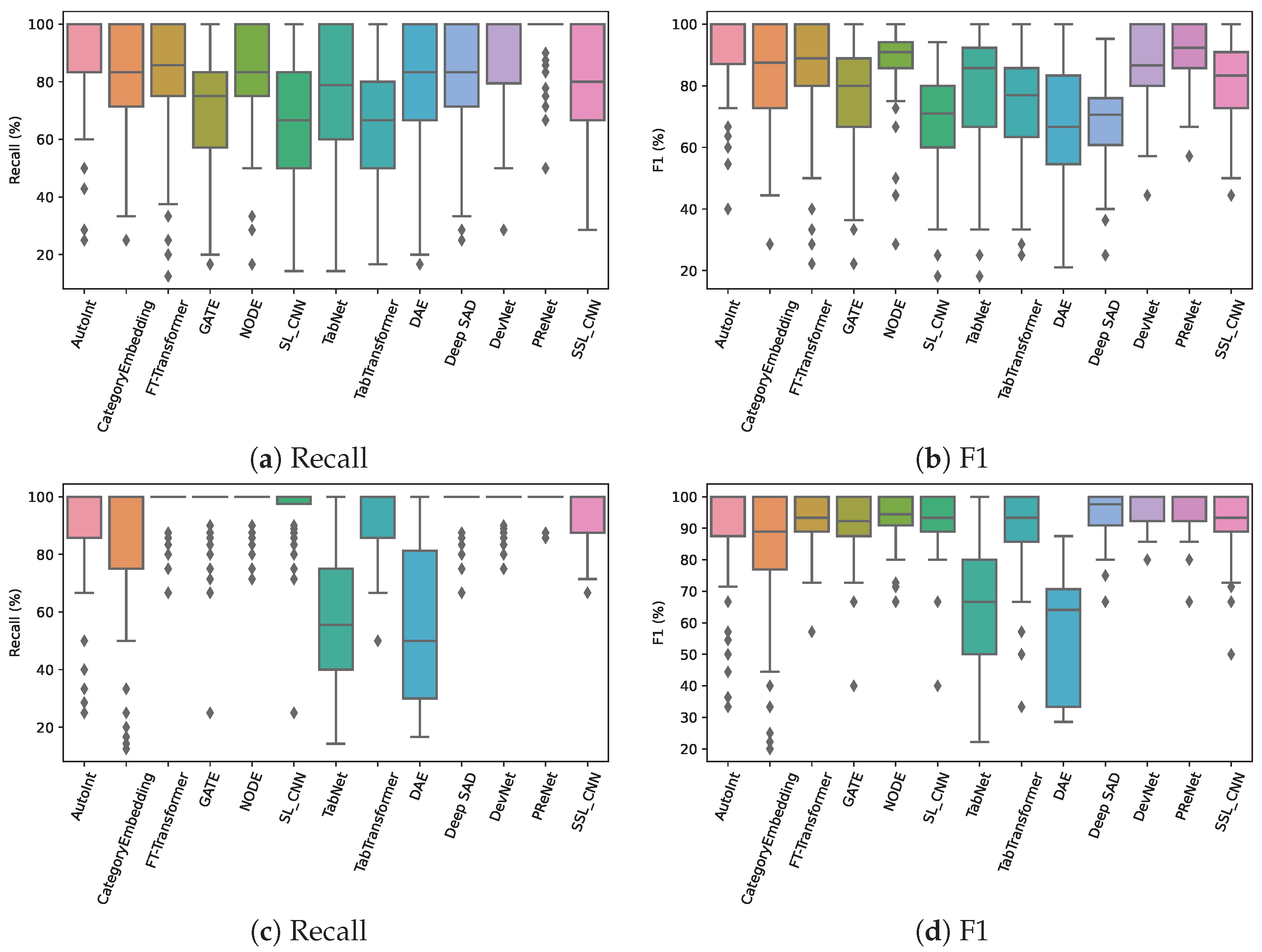
SSL_CNN	87.40 ± 8.57	86.99 ± 15.45	78.84 ± 17.28	80.72 ± 12.43

and 

Table 2. Comparison results (average ± standard deviation %) of 13 supervised (top) and semi-supervised (bottom) models on the simulated dataset. The best results are in bold. For all metrics, the higher, the better.

Model	Accuracy	Precision	Recall	F1
AutoInt	94.18 ± 8.60	92.29 ± 12.80	89.36 ± 19.64	90.07 ± 16.32
CategoryEmbedding	89.94 ± 10.12	84.73 ± 17.66	84.20 ± 24.02	82.34 ± 20.36
FT-Transformer	95.20 ± 4.92	88.76 ± 12.12	98.63 ± 5.29	92.97 ± 7.87
GATE	94.24 ± 5.54	88.50 ± 12.08	95.82 ± 10.46	91.15 ± 10.25
NODE	96.24 ± 4.36	92.92 ± 10.01	96.55 ± 7.54	94.25 ± 6.94
SL_CNN	95.71 ± 4.31	92.20 ± 11.57	94.98 ± 10.64	92.66 ± 9.27
TabNet	79.93 ± 12.51	87.09 ± 19.34	55.72 ± 25.18	63.55 ± 20.85
TabTransformer	93.81 ± 6.00	89.38 ± 13.40	92.68 ± 11.35	90.54 ± 11.21
DAE	75.00 ± 14.23	83.35 ± 25.97	55.65 ± 30.39	58.01 ± 20.75
Deep SAD	96.35 ± 4.30	92.05 ± 10.29	97.91 ± 6.01	94.53 ± 6.97
DevNet	97.53 ± 3.13	95.95 ± 7.38	97.47 ± 6.06	96.40 ± 4.74
PReNet	97.76 ± 3.09	94.07 ± 9.30	99.73 ± 1.88	96.54 ± 5.48
SSL_CNN	95.29 ± 4.92	92.87 ± 11.43	94.01 ± 9.02	92.80 ± 8.47

present the results of 13 models on the real-world and simulated datasets, respectively. The first conclusion to draw from both datasets is that no single model consistently outperforms all others across all evaluation metrics. However, regarding recall and F1, semi-supervised models generally outperform supervised models. The reason is that in the semi-supervised manner, unlabeled data are additionally added to the training process, providing the models with a broader understanding of data features. Compared to the others, NODE demonstrates relative superiority on both datasets among all supervised models, while PReNet outperforms all semi-supervised models. In the case of NODE, as introduced in Section 3.3, it is a deep neural network with each layer including an ensemble of decision trees. Decision trees are known for their ability to capture complex correlations between features in a dataset and identify feature importance. Ensemble learning is widely adopted in machine learning algorithms for its capacity to improve predictive performance by aggregating outputs of multiple base models. The combination of decision trees and ensemble learning has been proven to be powerful in various classification tasks [36,37]. In the case of PReNet, regardless of the architecture, the main difference between it and other semi-supervised models is that it further augments the data size by creating data pairs from any two randomly selected samples. This allows the model to leverage a more diverse training set and capture the difference between normal and abnormal data.

Figure 8 uses the box plots to display the five-number (minimum, first quartile, median, third quartile, and maximum) summary of experiments that have been run 100 times. In terms of recall, PReNet achieves nearly 100% in most experiments on both datasets, while NODE only exhibits competitive results on the simulated dataset. In terms of F1, on average, the difference between NODE and PReNet is less than 2% as shown in Table 1 and Table 2. However, the box plots show that NODE performs poorly (≤60% in many experiments on the real-world dataset). In addition, lower values of standard deviation in Table 1 and Table 2 indicate that a model has a more stable performance. The results show that PReNet outperforms others to this end.

In real-world scenarios, a DL-based detection model is deployed considering that the inference time is more important than the training time and the inference time is usually negligible in advanced DL frameworks and libraries, as well as hardware accelerators like GPUs and TPUs (i.e., Tensor Processing Units). As shown in

Table 3. Execution time (seconds) per instance of DL models in the reference time.

Model	Real-World	Simulated
AutoInt	2.91 $\times {10}^{-3}$	3.01 $\times {10}^{-3}$
CategoryEmbedding	1.46 $\times {10}^{-3}$	1.61 $\times {10}^{-3}$
FT-Transformer	4.05 $\times {10}^{-3}$	3.98 $\times {10}^{-3}$
GATE	7.46 $\times {10}^{-3}$	7.10 $\times {10}^{-3}$
NODE	3.96 $\times {10}^{-2}$	3.96 $\times {10}^{-2}$
SL_CNN	2.88 $\times {10}^{-4}$	3.76 $\times {10}^{-4}$
TabNet	2.26 $\times {10}^{-3}$	2.20 $\times {10}^{-3}$
TabTransformer	2.33 $\times {10}^{-3}$	2.34 $\times {10}^{-3}$
DAE	1.30 $\times {10}^{-3}$	1.28 $\times {10}^{-3}$
Deep SAD	7.57 $\times {10}^{-5}$	3.71 $\times {10}^{-5}$
DevNet	1.64 $\times {10}^{-3}$	3.79 $\times {10}^{-5}$
PReNet	1.53 $\times {10}^{-3}$	8.59 $\times {10}^{-4}$
SSL_CNN	4.38 $\times {10}^{-4}$	2.86 $\times {10}^{-4}$

, the execution time for predicting an instance is fast, often falling within the milliseconds range.

4.2.2. Impact Analysis of the Size of Unlabeled Data

The impact of the size of unlabeled data on semi-supervised models is analyzed here. The unlabeled set is randomly selected from all available data.

Table 4. Results (average ± standard deviation %) of four semi-supervised models on the real-world dataset using different sizes of unlabeled data. The last column is using all available unlabeled data. For each model, the best results over all sizes are in bold. For all metrics, the higher, the better.

Model	Size of Unlabeled Data (n Times of Labeled Training Data)
	1	10	50	100	200	300	>339
Accuracy
Deep SAD	73.70 ± 11.10	68.90 ± 13.03	81.10 ± 10.57	65.30 ± 14.73	78.80 ± 11.69	77.70 ± 11.48	74.33 ± 9.06
DevNet	91.10 ± 7.86	98.40 ± 3.93	93.00 ± 7.14	97.10 ± 5.88	93.00 ± 7.14	93.10 ± 7.17	91.53 ± 6.93
PReNet	87.80 ± 8.90	90.10 ± 7.81	86.30 ± 9.45	89.80 ± 7.61	92.90 ± 6.97	92.20 ± 7.95	93.18 ± 5.62
SSL_CNN	81.47 ± 7.86	80.41 ± 7.72	81.76 ± 7.46	83.88 ± 7.74	84.12 ± 7.46	81.41 ± 8.27	87.40 ± 8.57
Precision
Deep SAD	89.93 ± 18.48	77.69 ± 26.31	68.70 ± 17.37	69.30 ± 27.73	65.09 ± 18.21	64.40 ± 17.98	60.17 ± 15.94
DevNet	100	100	94.30 ± 11.10	99.15 ± 4.83	94.05 ± 11.26	94.05 ± 11.26	88.53 ± 12.04
PReNet	93.31 ± 11.77	91.99 ± 12.81	79.28 ± 17.05	91.61 ± 12.55	84.64 ± 15.35	83.73 ± 16.73	86.25 ± 11.47
SSL_CNN	80.22 ± 18.28	78.55 ± 20.09	83.42 ± 17.41	84.59 ± 16.97	85.72 ± 17.24	81.95 ± 17.41	86.99 ± 15.45
Recall
Deep SAD	43.07 ± 17.85	42.69 ± 19.35	90.76 ± 14.15	44.26 ± 21.01	90.91 ± 15.15	90.81 ± 14.73	81.24 ± 17.47
DevNet	77.07 ± 18.39	96.14 ± 9.53	87.34 ± 16.92	93.66 ± 14.30	87.68 ± 16.84	87.93 ± 16.83	86.98 ± 16.68
PReNet	76.31 ± 19.35	85.03 ± 16.35	89.71 ± 14.14	84.00 ± 17.09	99.32 ± 4.07	99.46 ± 3.07	97.28 ± 8.02
SSL_CNN	68.80 ± 19.15	67.28 ± 18.45	62.86 ± 19.11	71.84 ± 16.13	70.56 ± 19.09	65.16 ± 19.30	78.84 ± 17.28
F1
Deep SAD	54.95 ± 15.78	50.88 ± 17.14	76.68 ± 13.30	49.10 ± 16.87	74.35 ± 15.06	73.56 ± 14.27	67.55 ± 13.63
DevNet	85.82 ± 11.91	97.76 ± 5.61	89.17 ± 11.30	95.53 ± 9.76	89.22 ± 11.26	89.37 ± 11.31	86.53 ± 12.10
PReNet	81.93 ± 12.23	86.63 ± 10.43	82.69 ± 12.23	85.78 ± 10.26	90.57 ± 9.89	89.90 ± 10.78	90.93 ± 8.16
SSL_CNN	70.81 ± 13.51	69.33 ± 12.73	69.07 ± 13.80	75.21 ± 11.22	74.40 ± 13.65	69.51 ± 13.96	80.72 ± 12.43

shows the results of four semi-supervised models, Deep SAD, DevNet, PReNet, and SSL_CNN. DAE is excluded due to its low performance listed in Table 1.

Overall, only the SSL_CNN demonstrates a persistent trend, wherein an increase in unlabeled data leads to improvements across all metrics. Deep SAD exhibits particularly ad hoc behaviour, as optimal scores across different metrics are achieved with varying sizes of unlabeled data. DevNet consistently achieves its optimal performance when the unlabeled data are 50 times the size of labeled data. Beyond this size, however, performance starts to degrade. The reason might be that the capacity of DevNet to learn is overwhelmed by the large amount of data, leading to overfitting. PReNet demonstrates some regular behaviour; namely, Precision degrades with more unlabeled data but all other metrics improve with more unlabeled data.

Regarding the most relevant metrics, namely Recall and F1, DevNet and PReNet showcase competitive performances. Yet, we conjecture that PReNet’s performance could be further enhanced with an increase in the volume of available unlabeled data. In real-world scenarios, when unlabeled data are scarce, opting for DevNet is recommended, whereas PReNet excels when acquiring unlabeled data is effortless. Nevertheless, the selection of an appropriate set of unlabeled data remains a crucial factor to be considered.

5. Conclusions

In this work, we have focused on the performances of 13 deep learning (DL) models for the detection of SMS interception attacks that use “update location” call flows. Our empirical study has demonstrated that, generally, semi-supervised learning models can achieve better performance than supervised learning models for anomaly detection. On the other hand, supervised learning models can provide better performance when accuracy and precision are more important for some other application scenarios (i.e., the abnormal and normal cases in the dataset are balanced). Among semi-supervised models, PReNet stands out as the best regarding the recall and F1 metrics when all unlabeled data are used for training. Importantly, this model is also stable on both datasets and seems to be the best solution among all studied models. Furthermore, our impact analysis reveals that the size of unlabeled data has an impact on semi-supervised models. Among the four semi-supervised models (Deep SAD, DevNet, PReNet, and SSL_CNN), DevNet tends to overfit with a small volume of unlabeled data, while PReNet outperforms others with an increase of unlabeled data.

Following this work, many interesting research topics remain open, with some examples below. One is to further validate the results on larger datasets, potentially from different Telecom service providers. The second is to explore the selection of appropriate unlabeled data for semi-supervised models. The third is to expand the scope of attack detection to the different attacks that target Cat. 3 messages. It is an interesting topic to see how DL solutions generalise to broader attack categories.

References

- Tang, Q.; Ermis, O.; Nguyen, C.D.; Oliveira, A.D.; Hirtzig, A. A systematic analysis of 5G networks with a focus on 5G core security. IEEE Access 2022, 10, 18298–18319. [Google Scholar] [CrossRef]
- ENISA. Signalling Security in Telecom SS7/Diameter/5G. 2018. Available online: https://www.enisa.europa.eu/publications/signalling-security-in-telecom-ss7-diameter-5g (accessed on 11 September 2023).
- Metzler, J. Security Implications of 5G Networks. 2020. Available online: https://cltc.berkeley.edu/wp-content/uploads/2020/09/Security_Implications_5G.pdf (accessed on 11 September 2023).
- Kim, H. 5G core network security issues and attack classification from network protocol perspective. J. Internet Serv. Inf. Secur. 2020, 10, 1–15. [Google Scholar] [CrossRef]
- Ullah, K.; Rashid, I.; Afzal, H.; Iqbal, M.M.W.; Bangash, Y.A.; Abbas, H. SS7 vulnerabilities—A survey and implementation of machine learning vs. rule based filtering for detection of SS7 network attacks. IEEE Commun. Surv. Tutor. 2020, 22, 1337–1371. [Google Scholar] [CrossRef]
- Kristoffer, J. Improving SS7 Security Using Machine Learning Techniques. Master’s Thesis, Department of Computer Science and Media Technology, Norwegian University of Science and Technology, Trondheim, Norway, 2016. [Google Scholar]
- Hoang, T.H.T. Improving Security in Telecom Networks with Deep Learning Based Anomaly Detection. Master’s Thesis, Faculty of Science, Technology and Communication, University of Luxembourg, Esch-sur-Alzette, Luxembourg, 2021. [Google Scholar]
- Ermis, O.; Feltus, C.; Tang, Q.; Trang, H.; De Oliveira, A.; Nguyen, C.D.; Hirtzig, A. A CNN-based semi-supervised learning approach for the detection of SS7 attacks. In Proceedings of the Information Security Practice and Experience: 17th International Conference, Taipei, Taiwan, 23–25 November 2022; Springer: Berlin/Heidelberg, Germany, 2022; pp. 345–363. [Google Scholar] [CrossRef]
- Pang, G.; Shen, C.; Jin, H.; van den Hengel, A. Deep weakly supervised anomaly detection. In Proceedings of the 29th ACM SIGKDD Conference on Knowledge Discovery and Data Mining, Long Beach, CA, USA, 6–10 August 2023; Association for Computer Machinery: New York, NY, USA, 2023; pp. 1795–1807. [Google Scholar] [CrossRef]
- Popov, S.; Morozov, S.; Babenko, A. Neural oblivious decision ensembles for deep learning on tabular data. In Proceedings of the International Conference on Learning Representations, Online, 26 April–1 May 2020. [Google Scholar]
- Positive Technologies. SS7 Vulnerabilities and Attack Exposure Report. 2018. Available online: https://www.gsma.com/membership/wp-content/uploads/2018/07/SS7_Vulnerability_2017_A4.ENG_.0003.03.pdf (accessed on 11 September 2023).
- GSMA Association. IR.82 SS7 Security Network Implementation Guidelines v5. 2016. Available online: https://www.gsma.com/security/resources/ir-82-ss7-security-network-implementation-guidelines-v5-0/ (accessed on 11 September 2023).
- Fouladi, R.F.; Ermiş, O.; Anarim, E. A DDoS attack detection and countermeasure scheme based on DWT and auto-encoder neural network for SDN. Comput. Netw. 2022, 214, 109140. [Google Scholar] [CrossRef]
- Fouladi, R.F.; Ermiş, O.; Anarim, E. A novel approach for distributed denial of service defense using continuous wavelet transform and convolutional neural network for software-Defined network. Comput. Secur. 2022, 112, 102524. [Google Scholar] [CrossRef]
- Ahmed, M.; Naser Mahmood, A.; Hu, J. A survey of network anomaly detection techniques. J. Netw. Comput. Appl. 2016, 60, 19–31. [Google Scholar] [CrossRef]
- Wang, S.; Balarezo, J.F.; Kandeepan, S.; Al-Hourani, A.; Chavez, K.G.; Rubinstein, B. Machine learning in network anomaly detection: A survey. IEEE Access 2021, 9, 152379–152396. [Google Scholar] [CrossRef]
- Villa-Pérez, M.E.; Álvarez Carmona, M.A.; Loyola-González, O.; Medina-Pérez, M.A.; Velazco-Rossell, J.C.; Choo, K.K.R. Semi-supervised anomaly detection algorithms: A comparative summary and future research directions. Knowl.-Based Syst. 2021, 218, 106878. [Google Scholar] [CrossRef]
- Cheplygina, V.; de Bruijne, M.; Pluim, J.P. Not-so-supervised: A survey of semi-supervised, multi-instance, and transfer learning in medical image analysis. Med. Image Anal. 2019, 54, 280–296. [Google Scholar] [CrossRef] [PubMed]
- Kiran, B.R.; Thomas, D.M.; Parakkal, R. An overview of deep learning based methods for unsupervised and semi-supervised anomaly detection in videos. J. Imaging 2018, 4, 36. [Google Scholar] [CrossRef]
- Cui, Y.; Liu, Z.; Lian, S. A survey on unsupervised anomaly detection algorithms for industrial images. IEEE Access 2023, 11, 55297–55315. [Google Scholar] [CrossRef]
- Jensen, K.; Do, T.V.; Nguyen, H.T.; Arnes, A. Better protection of SS7 networks with machine learning. In Proceedings of the 6th International Conference on IT Convergence and Security (ICITCS), Prague, Czech Republic, 26 September 2016; pp. 1–7. [Google Scholar] [CrossRef]
- Rezaei, S.; Liu, X. How to achieve high classification accuracy with just a few labels: A semi-supervised approach using sampled packets. arXiv 2018, arXiv:1812.09761. [Google Scholar]
- Jensen, K.P. SS7 Attack Simulator Based on RestComm’s jss7. Available online: https://github.com/polarking/jss7-attack-simulator (accessed on 11 September 2023).
- Song, W.; Shi, C.; Xiao, Z.; Duan, Z.; Xu, Y.; Zhang, M.; Tang, J. AutoInt: Automatic feature interaction learning via self-attentive neural networks. In Proceedings of the 28th ACM International Conference on Information and Knowledge Management, CIKM ’19, Beijing, China, 3–7 November 2019; Association for Computer Machinery: New York, NY, USA, 2019; pp. 1161–1170. [Google Scholar] [CrossRef]
- Vaswani, A.; Shazeer, N.; Parmar, N.; Uszkoreit, J.; Jones, L.; Gomez, A.N.; Kaiser, L.u.; Polosukhin, I. Attention is all you need. In Proceedings of the 31st Conference on Neural Information Processing Systems, Long Beach, CA, USA, 4–9 December 2017; Guyon, I., Luxburg, U.V., Bengio, S., Wallach, H., Fergus, R., Vishwanathan, S., Garnett, R., Eds.; Curran Associates, Inc.: Red Hook, NY, USA, 2017; Volume 30. [Google Scholar]
- Joseph, M. PyTorch tabular: A framework for deep learning with tabular data. arXiv 2021, arXiv:2104.13638. [Google Scholar]
- Gorishniy, Y.; Rubachev, I.; Khrulkov, V.; Babenko, A. Revisiting deep learning models for tabular data. In Proceedings of the Advances in Neural Information Processing Systems, Online, 6–14 December 2021; Beygelzimer, A., Dauphin, Y., Liang, P., Vaughan, J.W., Eds.; Neural Information Processing Systems: San Diego, CA, USA, 2021. [Google Scholar]
- Joseph, M.; Raj, H. GATE: Gated additive tree ensemble for tabular classification and regression. arXiv 2023, arXiv:2207.08548. [Google Scholar]
- Cho, K.; van Merriënboer, B.; Gulcehre, C.; Bahdanau, D.; Bougares, F.; Schwenk, H.; Bengio, Y. Learning phrase representations using RNN encoder–decoder for statistical machine translation. In Proceedings of the 2014 Conference on Empirical Methods in Natural Language Processing (EMNLP), Doha, Qatar, 25–29 October 2014; pp. 1724–1734. [Google Scholar] [CrossRef]
- Arik, S.O.; Pfister, T. TabNet: Attentive interpretable tabular learning. Proc. AAAI Conf. Artif. Intell. 2021, 35, 6679–6687. [Google Scholar] [CrossRef]
- Huang, X.; Khetan, A.; Cvitkovic, M.; Karnin, Z. TabTransformer: Tabular data modeling using contextual embeddings. arXiv 2020, arXiv:2012.06678. [Google Scholar]
- Vincent, P.; Larochelle, H.; Bengio, Y.; Manzagol, P.A. Extracting and composing robust features with denoising autoencoders. In Proceedings of the 25th International Conference on Machine Learning, ICML ’08, Helsinki, Finland, 5–9 July 2008; Association for Computing Machinery: New York, NY, USA, 2008; pp. 1096–1103. [Google Scholar] [CrossRef]
- Ruff, L.; Vandermeulen, R.A.; Görnitz, N.; Binder, A.; Müller, E.; Müller, K.R.; Kloft, M. Deep semi-supervised anomaly detection. In Proceedings of the International Conference on Learning Representations, Online, 26 April–1 May 2020. [Google Scholar]
- Ruff, L.; Vandermeulen, R.; Goernitz, N.; Deecke, L.; Siddiqui, S.A.; Binder, A.; Müller, E.; Kloft, M. Deep one-class classification. Proc. Mach. Learn. Res. 2018, 80, 4393–4402. [Google Scholar]
- Pang, G.; Shen, C.; van den Hengel, A. Proceedings of the 25th ACM SIGKDD International Conference on Knowledge Discovery & Data Mining, KDD ’19, Anchorage, AK, USA, 4–8 August 2019; Association for Computing Machinery: New York, NY, USA, 2019; pp. 353–362. [CrossRef]
- Che, D.; Liu, Q.; Rasheed, K.; Tao, X. Decision tree and ensemble learning algorithms with their applications in bioinformatics. In Software Tools and Algorithms for Biological Systems; Springer: New York, NY, USA, 2011; pp. 191–199. [Google Scholar] [CrossRef]
- Webb, G.I.; Zheng, Z. Multistrategy ensemble learning: Reducing error by combining ensemble learning techniques. IEEE Trans. Knowl. Data Eng. 2004, 16, 980–991. [Google Scholar] [CrossRef]
- Xu, H. DeepOD: Python Deep Outlier/Anomaly Detection. 2023. Available online: https://github.com/xuhongzuo/DeepOD (accessed on 11 September 2023).
Figure 1.
Mobile subscribers (in billions) by technology 2016–2027 (expected). Figure source: https://tinyurl.com/4wze6un5 (accessed on 11 September 2023).
Figure 2.
Holistic view of 2G/3G core networks.
Figure 3.
Percentage of successful attacks against SS7 with respect to message categories based on the presence of a filtering-based defense mechanism (Credit: [11]).
Figure 4.
The update location call flow in the SS7 protocol and SMS interception attack using update location (Credit: [8]).
Figure 5.
Overview of the empirical study.
Figure 6.
Mutual information and mean absolute difference results on a labeled real-world dataset.
Figure 7.
Example of positive and negative instances.
Figure 8.
Comparison results of 13 models on the real-world (top) and simulated (bottom) datasets visualized using a box plot. For all metrics, the higher, the better.