
Multi-Sensor Fusion Target Tracking Based on Maximum Mixture Correntropy in Non-Gaussian Noise Environments with Doppler Measurements

School of Astronautics and Aeronautics, Shanghai Jiao Tong University, Shanghai 200240, China
*
Author to whom correspondence should be addressed.
Information 2023, 14(8), 461; https://doi.org/10.3390/info14080461
Submission received: 10 July 2023
/
Revised: 4 August 2023
/
Accepted: 10 August 2023
/
Published: 15 August 2023
Abstract
:This paper addresses the multi-sensor fusion target tracking problem based on maximum mixture correntropy in non-Gaussian noise environments exclusively using Doppler measurements. As Doppler measurements are non-linear, a statistical linear regression model is constructed using the unscented transformation. Then, a centralized measurement model is developed, and the mixture correntropy is determined, which contains the high-order statistics of state prediction and the measurement error caused by noise. Then, a robust fusion filter is proposed by maximizing the mixture-correntropy-based cost. To improve numerical stability, the information filter and corresponding square root version are also derived. Furthermore, the performance of the proposed algorithm is analyzed, and the selection of the kernel width is discussed. Experiments are performed using simulated data and automatic driving software. The results show that the estimation performance of the proposed algorithm is better with respect to outliers and mixture Gaussian noise than that of traditional methods.
1. Introduction
Doppler tracking is a technique that is widely used in the fields of radar, wireless communication, and acoustics, and it is also used for the motion state tracking of targets. In this technique, by employing the Doppler effect, the speed and direction of the movement of a target are inferred by analyzing the frequency variation of the received signal. Doppler tracking plays an important and well-established role in radar systems: it can help a radar system to detect and track moving targets in real time. Doppler tracking offers the advantages of high-precision speed measurement, motion state estimation, real-time performance, anti-interference ability, and wide applicability. These properties make it an important technique for object tracking and motion analysis in many fields [1,2].
To solve a target-tracking problem using Doppler measurements, Ristic and Farina implemented Bernoulli PF for Doppler tracking in multi-static situations in [3]. These authors utilized fixed single-transmitter and Doppler measurements measured by multiple receivers in order to jointly detect and track targets. As the Doppler measurements were non-linear, the solution was obtained via particle implementation. Ristic and Farina also proposed an active receiver-based approach in [4] to improve the information collected from sensors, and to discard measurements from sensors aligned with the target and transmitter in the bistatic case. This study shows that the choice of receiver improves track-settling time and steady-state error performance. The observability and performance of dual/multistatic Doppler radars were analyzed by Xiao in [5]. For simplicity, the author analyzed the multi-transmitter-receiver case, and pointed out that this case can also be generalized to multi-transmitter and multi-receiver cases. In the case of a single receiver, observability is evaluated using the rank of the Fisher Information Matrix (FIM). If a target is completely observable, the FIM should have the highest rank. These Doppler-tracking filter methods and analyses for target tracking are all based on Gaussian assumptions.
A Kalman filter (KF) is an optimal estimator under the minimum mean square error criterion, for which a solution is achieved by recursively updating the estimated state and covariance matrix based on a state-space model. For nonlinear systems, various sub-optimal nonlinear extensions have been proposed. However, with respect to dealing with non-Gaussian noise, such as impulsive interference or outliers, their estimation performance is poor, as the minimum mean square error cannot indicate the bias of the predicted state. Accordingly, Robust filters, such as the filter and Huber’s filter [6,7,8], are employed in this situation. In particular, the filter ensures bounded estimation error but performs poorly in relation to Gaussian noise. Alternatively, Huber’s filter is suitable for dealing with data estimation problems involving outliers. Based on the theory of robust statistics, Huber’s filter has a certain robustness to outliers, and it can resist the interference of outliers. The Huber–Kalman filter can be used to obtain optimal results by minimizing a combined and norm. Huber estimation can provide better estimation results in the presence of outliers, and it has a better fitting effect on non-outliers.
Recently, a new cost function based on information theory was constructed, and a corresponding optimal criterion was proposed [9]. Correntropy is defined as a local similarity measure, and it is used as a cost for state estimation [10]. By maximizing the correntropy-based cost, the maximum correntropy criterion (MCC) was employed to derive robust solutions. As correntropy costs contain the high-order statistics of the error signal, the high-order characteristics of the error distribution can be captured, and the derived solutions are, therefore, more robust. MCC-based Kalman filters (MCC-KFs) can be used to solve linear and non-linear state estimation problems involving non-Gaussian noise, such as outliers and impulsive noise, and the performance is obviously better than traditional methods [11,12]. In fact, MCC-based filters can also be treated as a smoothed MAP estimator [13]. However, MCC-based filters cannot be obtained in closed forms; therefore, the solutions are usually obtained using a fixed-point iteration approach [14]. The selection of kernel width is also important in MCC-based algorithms, as it determines the relative weighting of different orders of norms in the loss function, thus potentially altering the estimation results. In [15], the algorithm performance under different kernel widths was shown and analyzed; better estimation performance was obtained using an appropriate kernel width.
This paper addresses the problem of multi-sensor fusion target tracking in non-Gaussian noise environments with Doppler measurements based on maximum mixture correntropy. A statistical linear regression model is constructed for nonlinear ranges, angles, and Doppler measurements by employing unscented transformation. Based on the centralized measurement model, a mixture-correntropy-based cost function is constructed to capture the high-order statistics of state prediction and the measurement error that are caused by non-Gaussian noise. Subsequently, a robust fusion filter is developed by maximizing the cost function based on the maximum correntropy criterion. The solution is obtained through an iterative approach and the use of square roots. To enhance numerical stability, the information filter version is also derived. This paper also analyzes the performance of the proposed algorithm and discusses the selection of kernel width. Experiments are performed using numerical simulation and automatic driving software; the results demonstrate that the proposed method is more robust against non-Gaussian noise than conventional methods.
2. Background
2.1. Maximum Correntropy Criterion
Define is the error between two variables and with probability distribution . The information of the error can be measured according to the definition of Renyi’s entropy, which is denoted as:
where denotes the expectation operator. The variable is the order of the function. Therefore, Expression (1) is called Renyi’s entropy, and is information potential estimator.
When , the term is quadratic Renyi’s entropy:
Based on Expression (2), the correntropy can be defined as a generalized similarity measure between two random variables as follows:
where is a shift-invariant kernel function. Without loss of generality, the Gaussian kernel function is used in this paper, which is given by:
where , and is the kernel width.
Usually, the joint distribution is unknown, and only limited numbers of data are available. In this situation, the PDF can be estimated from data using Parzen’s window estimator, and the expectation operator can be approximated with the sample mean. The nonparametric estimation of quadratic information potential can be calculated as:
where represents the Gaussian kernel function. Based on the optimization theory, the optimal solution is obtained when the similarity of two variables is maximized with respect to , such as, for example:
This criterion is called the maximum correntropy criterion. Notice that the logarithm is dropped, and, therefore, the derivation of (6) is equal to maximize the term , such as, for example:
It can be seen that the term contains the high moments of the error. Thus, the MCC algorithm derives the optimal solution in high-dimensional space, and the results are more robust given non-Gaussian noise.
2.2. Doppler Measurement Equation
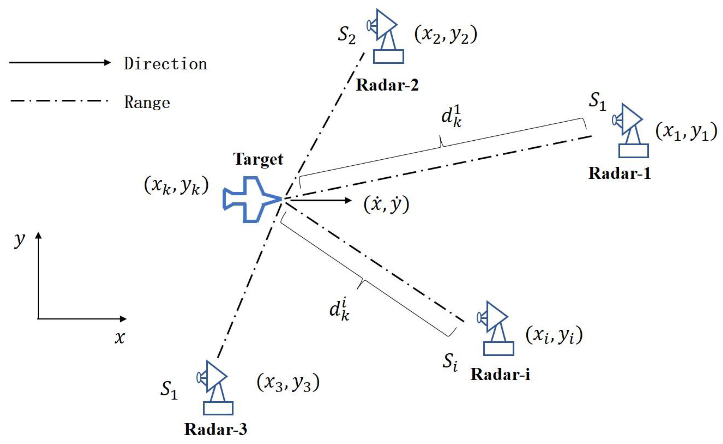
Consider the multi-radar fusion situational awareness background, assuming that the data fusion center knows the position of the transmitter and the sensor, the moving target detected by the sensor gives each Doppler measurement, and the sensor outputs the measured value to the data fusion center. The scene is illustrated in Figure 1:
Assume that the state vector of the target is a variable in space and can be denoted as , in which is the position of the target, are the speed, and the notation T represents the transpose operation.
The Doppler measurement is generated by each sensor in the scene, , and the motion of the target in the direction of the transmitter and receiver jointly cause the Doppler effect, which is located at the i-th of .The multi-static Doppler frequency shift measured by two sensors is taken in space , the measurement results are transmitted to the data fusion center, and the measurement equation shown in Formulas (3) and (4) are given as:
Among them, is the Doppler frequency shift, is the wavelength of the transmitted signal, and is the measurement noise of the sensor. The linearization matrix of can be expressed as:
and is the measurement noise of sensor :
3. Robust Fusion Filter Based on Maximum Mixture Correntropy
3.1. Mixture Correntropy Cost Function
Consider the discrete nonlinear state-space model:
where and are the nonlinear state transition equation and the nonlinear measurement equation with an independent non-linear process and a measurement noise of and with the associated covariance and . Assume that at time , the prior state is with the associated covariance , and the dimension of the state vector is . To approximate the nonlinear of the state transition process and the measurement, a set of sigma points are generated based on the unscented transform [16].
According to the state transition equation and the nonlinear measurement equations, the predicted sigma points , can be obtained, and the predicted state and the predicted measurement can then be calculated as:
Similarly, the predicted state covariance and the state-measurement cross-covariance matrix can then be calculated using the sigma points as:
Define the measurement slope matrix as:
Then, the measurement equation for sensor can be approximated by a statistical linear regression model as:
This equation is derived based on Kalman filtering equations [17], which provide the pseudo-measurement to approximate the nonlinear observation model for state update and filtering operations with unscented transformation. The pseudo-measurement is an approximate measure obtained by predicting a state estimate and linearizing the observation model in order to transform the nonlinear observation model into a linear model. Pseudo-measurements can help us to deal with both nonlinear and non-Gaussian noise in estimation problems.
Then, the centralized measurement equation [16] can be constructed as:
where the vector and matrix represent the augmented multi-source measurements and measurement matrix, respectively, and is the multi-source measurement noise vector with covariance .
Let , and the mixture correntropy between predicted state and measurements can then be defined as:
where is the th element of , is the selected kernel width for sensor according to the noise distribution characteristics, and is the dimension of the measurement for sensor .
Assuming independence between the dynamic process noise and the measurement noise, the MMC criteria are applied to the state transition and the measurement models. The optimal solution can be obtained by minimizing the combined cost function based on correntropy according to the maximum correntropy criterion:
where .
3.2. Robust Fusion Information Filter Based on Maximum Correntropy Criterion
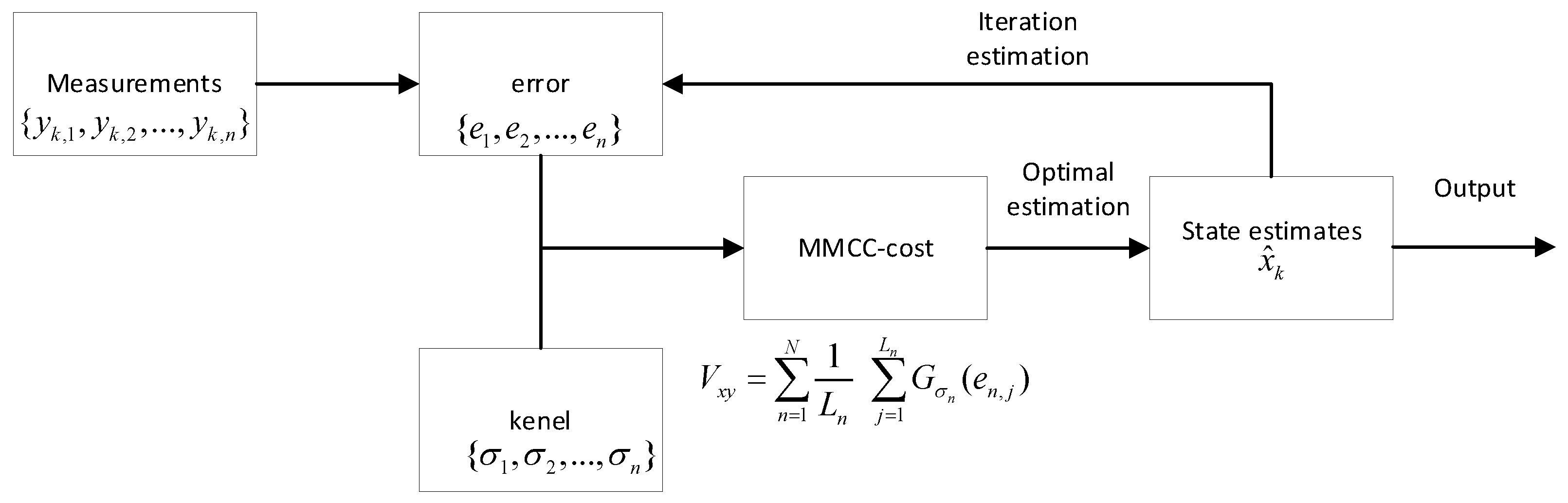
As shown in Figure 2, we provide the structural diagram of the proposed algorithm, which has a recursive framework. In this section, an iterative algorithm is proposed for multi-sensor fusion estimation with non-Gaussian noise. The mixture correntropy cost is constructed and recursively calculated as it related to the state estimates.
To improve the numerical stability, the fusion estimation algorithm within the information filter framework is proposed in this section.
Start with the Fisher information matrix and information vector at time , and the state estimate can be represented as and the associated covariance is . Then, the predicted state vector and associated covariance are calculated using (12) and (13).
Differentiating Equation (16) with respect to , the optimal estimate satisfies the equality:
where , and the term and are calculated as:
where is the th element of .
The posterior information matrix is:
and the posterior information vector is:
The detailed derivation is provided in Appendix A.
Then, the posterior state estimate is:
The state estimate is involved in the computation of , which implies that both sides of Equation (17) are interdependent with . In order to update the estimates in the Kalman filter, a fixed-point iteration approach is employed where the innovation covariance matrix and the posterior information matrix and vector are recalculated iteratively until convergence is achieved. Using the posterior estimate obtained from Equation (22), the terms and are recalculated, and the posterior information matrix and vector are updated iteratively.
The robust square root (SR) fusion information filter is a modification of the MCC-based fusion information filter using Cholesky factors. Then, re-formulate the filtering equations, and a more numerically stable algorithm will be derived than the original method.
The SR implementation of the fusion information filter uses QR factorization in each iteration step to update the corresponding Cholesky factors. This involves decomposing the information matrix into an orthogonal matrix Q and an upper triangular matrix R, such that . The Cholesky factor can also be computed using the QR factorization of , where T denotes the transpose operation.
Algorithm: Maximum mixture correntropy fusion filter:
(1) Initialize and vector of the target state, and the posterior covariance is then and the state vector is .
(2) Time update:
Evaluate the sigma points , and predict the points and predicted state values by using the process equation.
(3) Calculate the square root using QR decomposition:
Calculate and .
(4) Measurement update:
Calculate and the measurement slope matrix using the measurement equation to obtain the regression model (16).
(5) Compute the term using (19).
(6) Calculate the posterior information matrix:
where . Calculate the posterior information matrix and the information vector:
(7) Repeat steps 4–6 until convergence is achieved.
3.3. Analysis of the Algorithm Convergence
The kernel width is a crucial parameter, and the selection of this parameter affects the convergence of both the algorithm and the fusion estimation performance.
In this section, we analyze the effect of parameter selection on the convergence of the iteration implementation of the proposed algorithm. Since the MCC solution cannot be obtained in closed form, iterative methods are used to derive the final results. The convergence of the fixed point iteration approach is guaranteed by the compression mapping theorem when the function and its derivative are bounded. Here, we define as the upper bound of , and we ensure that the function satisfies this inequality:
where is the state dimension, is the 2-norm of matrix, is the th row of , and is the element of the vector . The term , where is the element of the vector . The inequality (a) and (c) hold according to the properties of the matrix norm, and the inequality (b) is established based on the triangle inequality. The inequality (d) holds as is a monotonically decreasing value of .
According to (26), we obtain a function of kernel width:
which satisfies . Moreover, when , , and when , the function . The reason is that the function is continuous and involves the monotonic decreasing of .
Therefore, the equation has the solution , and for any upper bound of , we have:
Differencing Equation (27) with respect to , when the kernel widths are large, we have:
When the selected kernel widths meet the conditions in (28) and (29) at the same time, the convergence of the fixed point iterative algorithm is guaranteed.
3.4. Discussion of the Kernel Selection
Further, we analyze the influence of parameter selection on estimation performance. Extend the potential estimator around zero by the Taylor series yields:
when the kernel width , the term can be approximated by the sum of zero order and first-order terms in Taylor expansion:
Then, the cost function in (19) is as follows:
which can be represented as follows:
where . This equation is the same as the traditional MMSE-based fusion cost function, and the derived solution is similar to the conventional Kalman filter fusion algorithm.
The kernel widths are crucial parameters in the maximum mixture correntropy (MMCC)-based fusion algorithm, and they can be set manually or optimized through trial-and-error in practical applications.
4. Simulation
4.1. Numerical Example
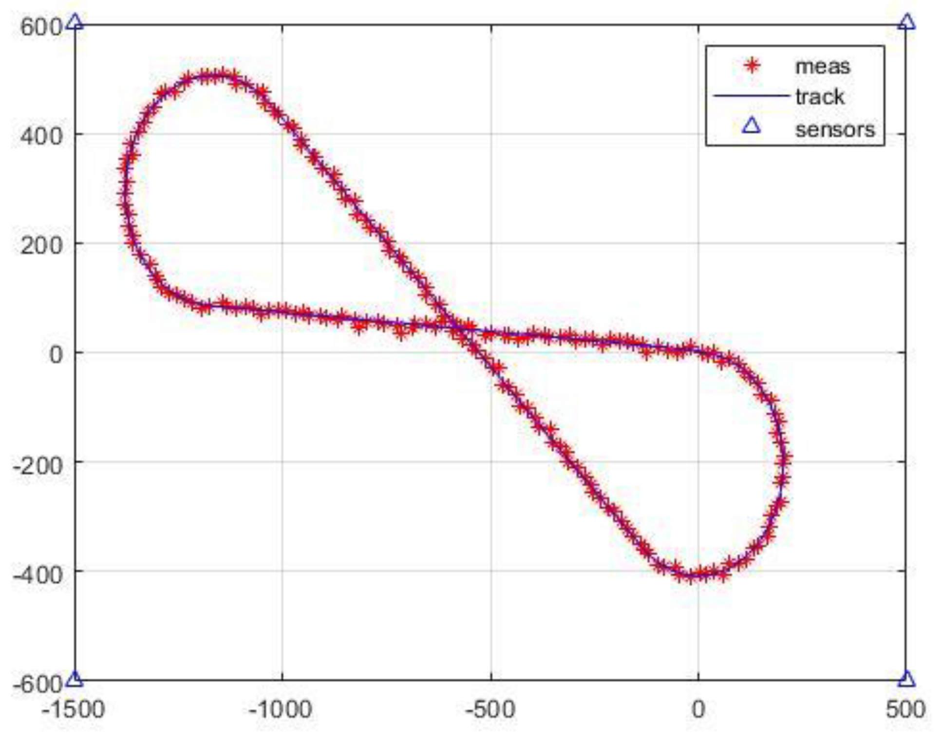
In this section, simulations are performed in order to demonstrate the effectiveness of the proposed algorithm, and they are then compared with traditional methods. In the scenario, consider linear constant velocity (CV) and nonlinear constant turn (CT) motion models with state transition equation:
where
for the CV model, and
for the CT model.
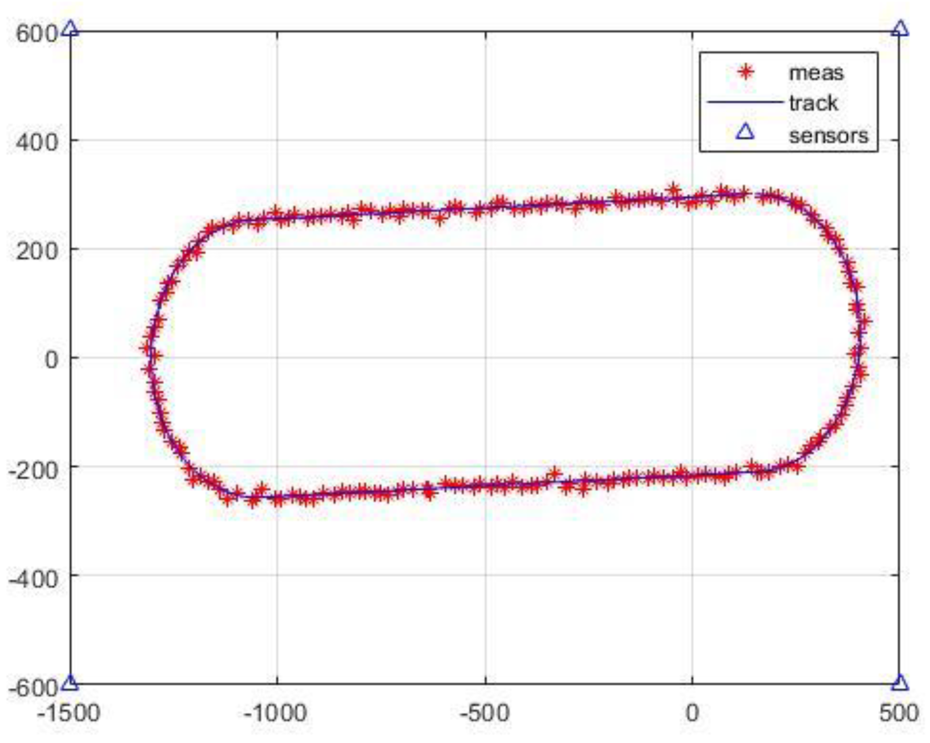
In the state transition matrix, the turn rate , and the dynamic state is initialed with . The target track is shown in Figure 3.
In these equations, represents the interval between the target motion and the measurements, which also corresponds to the time step of the iterative estimation process proposed in this paper. In practical applications, the target signal is accumulated within the interval, and Doppler measurements are obtained by Fourier transform. Since this paper mainly studies the fusion estimation method with target Doppler measurement under non-Gaussian measurement conditions, the radar signal processing is not discussed in detail here.
The process noise follows mixture Gaussian distribution:
and the covariance in the distribution can be represented as:
where , .
Four sensors receive Doppler measurements. As shown in Figure 1, the positions of the sensors are set at [−1500 m, −600 m], [−1500 m, 600 m], [500 m, −600 m], and [500 m, 600 m], respectively, and the measurement equation can be represented as:
When the radar carrier frequency is 1 GHz, consider four kinds of non-Gaussian measurement noise:
In these equations, the first kind of noise is Gaussian noise with covariance ; the second is Gaussian noise with outliers, in which the outliers are generated with probability 0.1 and covariance ; the third is mixture Gaussian noise with covariance , ; and the fourth is mixture Gaussian noise with outliers.
In the simulation, the initial position and the velocity estimates are calculated by the Doppler cross approach. The termination threshold of the iteration implementation is set to 0.01. The proposed MMCC-based fusion method is compared with the traditional fusion method based on KF [17] and the robust Huber filter [8] in terms of the root mean squared error (RMSE) with 200 Monte Carlo trails. The selection of kernel widths is crucial for the performance here, and these parameters are chosen based on the error distribution through trial-and-error.
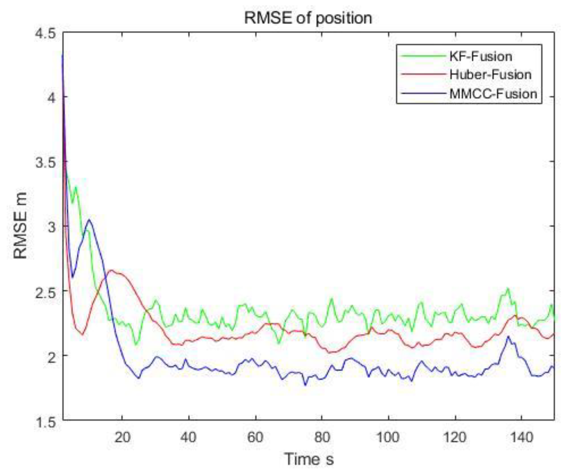
The fusion estimation results with Gaussian noise, mixture Gaussian noise, outliers, and complex noise are presented in Table 1, respectively. Appropriate kernel widths are selected in order to obtain the best performance for the correntropy-based fusion method. Figure 4 and Figure 5 show the estimation performance given mixture Gaussian noise and outliers. As shown in the figures, the MMCC-Fusion method outperforms the other algorithms. The reason for this is that the correntropy-based cost function in the MMCC-Fusion method captures higher-order statistics compared to the correction function in the Huber-Fusion algorithm, which allows it to accurately reflect the characteristics of the arbitrarily distributed process and the measurement noise. Therefore, the MMCC-Fusion-IF algorithm is able to effectively suppress different types of non-Gaussian noise under the MCC criterion. This experiment demonstrates the robustness and the adaptiveness of the correntropy-based method in complex non-Gaussian noise scenarios.
Table 1 provides the estimation performance given different noise patterns. It can be seen that KF is the optimal estimator, and that it performs best given Gaussian noise. However, the MMCC-Fusion method can still provide better results. The reason for this is that through select appropriate kernel width, relatively good results can be achieved under arbitrary noise conditions, and this also reflects the flexibility of the MMCC-based method. When the kernel width approaches infinity, the estimation results are close to the traditional Kalman filter fusion method.
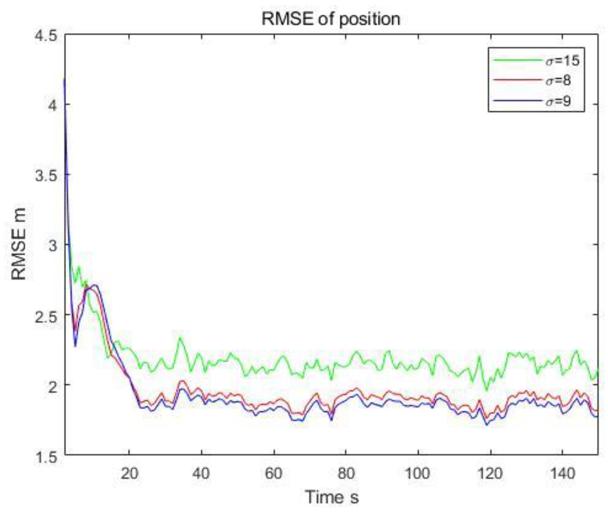
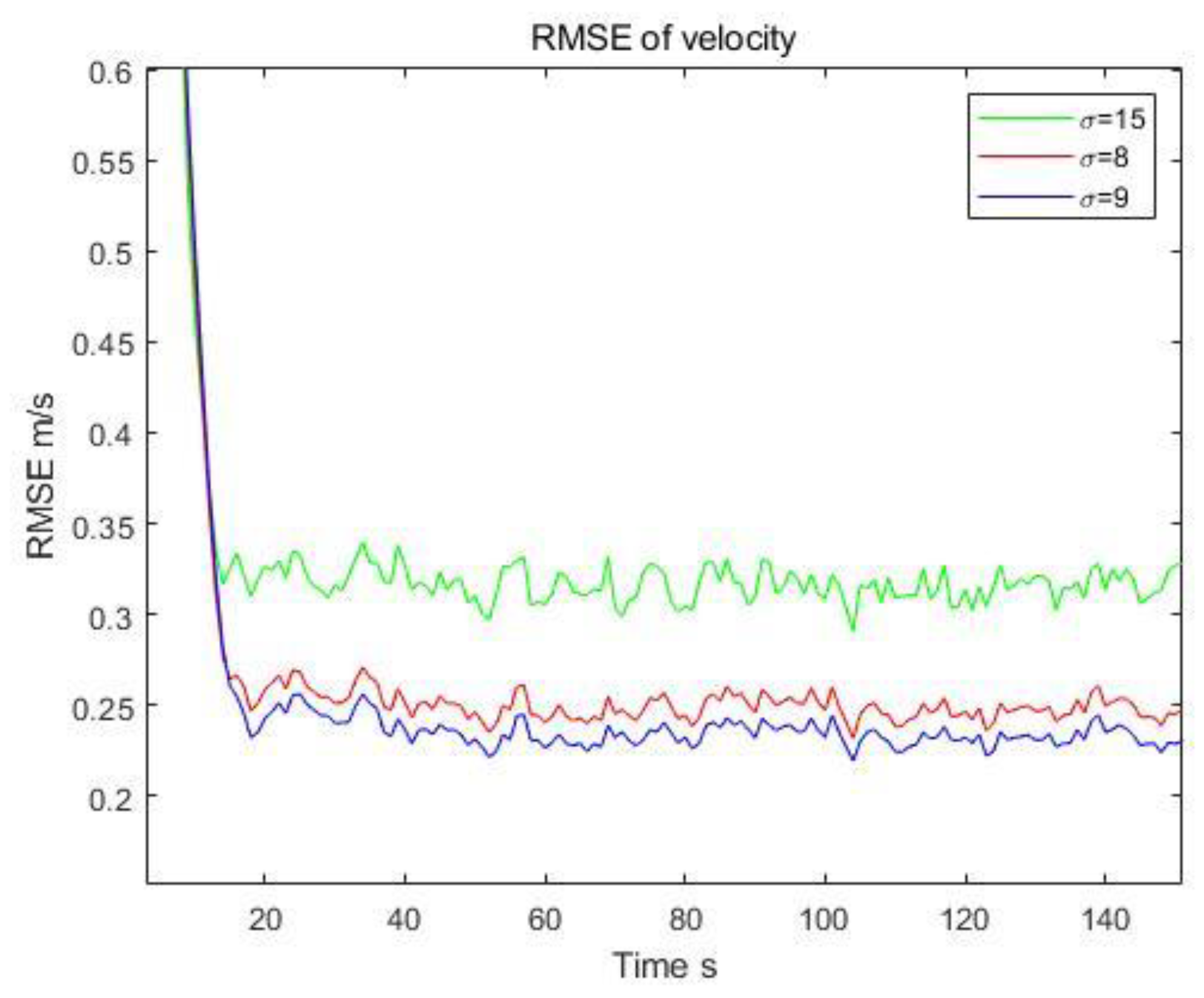
Evaluate the estimation performance with different kernel widths. Outliers generated with the parameters in case 2 are contained in the measurements. As shown in Figure 6 and Figure 7 and also listed in Table 2, the estimation results are the best when the kernel widths are selected as σ = 9 for each Doppler radar, which leads to a desirable error distribution and optimal results. It can be seen that the performance decreases with inappropriate kernel widths because the characteristics cannot be accurate captured. With the increasing of kernel width, the second moment of the error has the largest proportion in the correntropy-based loss function. In this situation, the loss function is approximate to the minimum mean square error loss, and the estimation results will be close to the traditional Kalman filter fusion.
Furthermore, Table 2 shows that larger kernel widths result in faster convergence. With kernel widths larger than 10, the iterative implementation of the proposed algorithm converges to the optimal solution quickly in only two or three iterations. Therefore, very small kernel widths should be avoided to avoid slow convergence.
4.2. Autonomous Driving Data Simulation
This experiment provided the tracking of an autonomous driving vehicle. The data source is from the Udacity course self-driving car [18], and the Doppler measurements are obtained by four distributed radar sensors. The track of the car is shown in Figure 8:
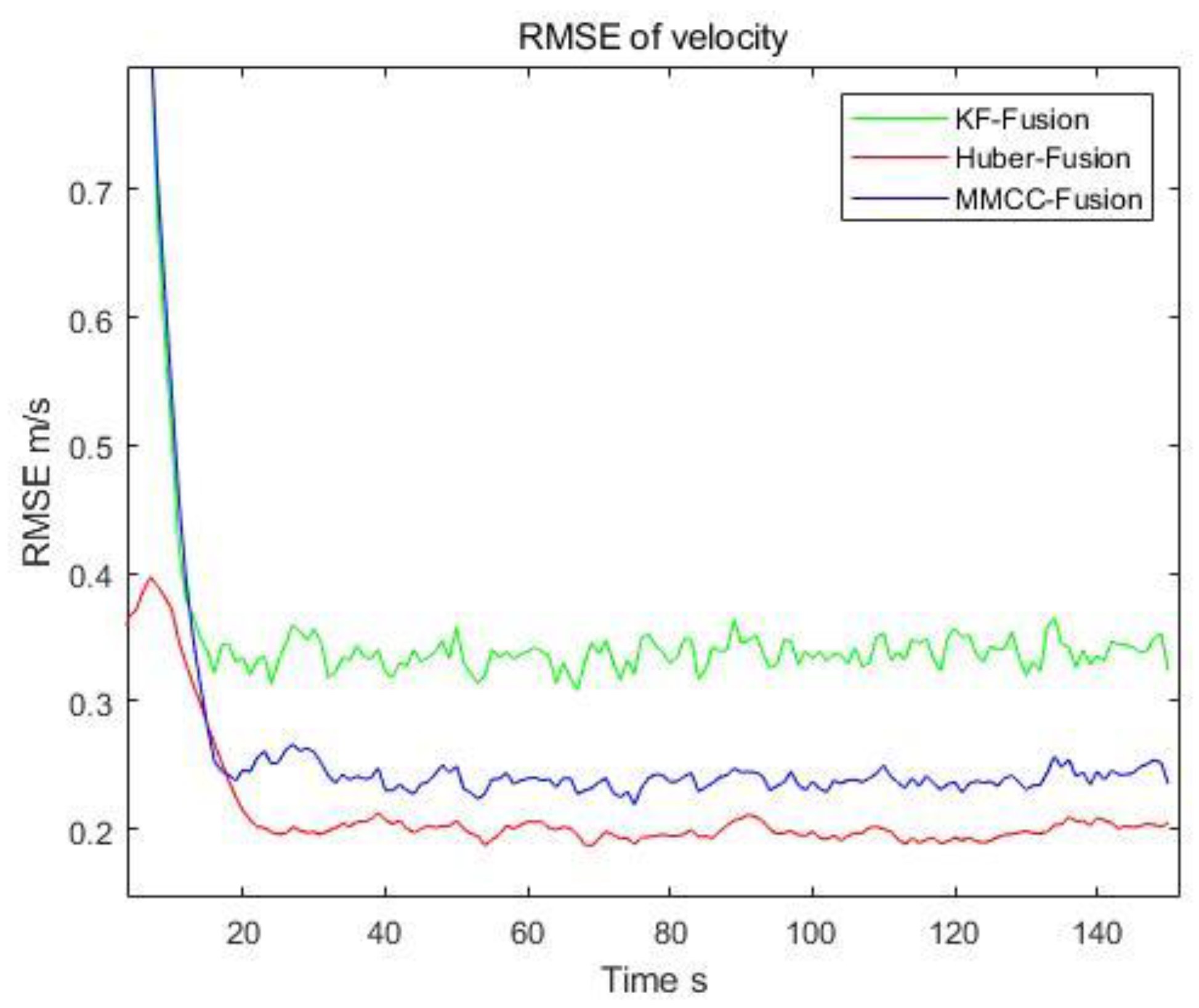
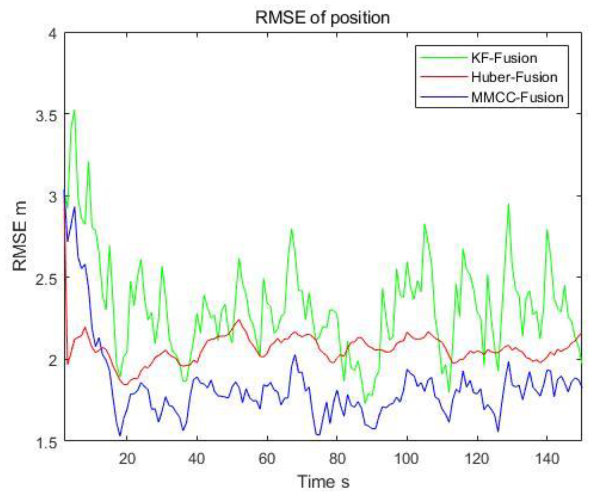
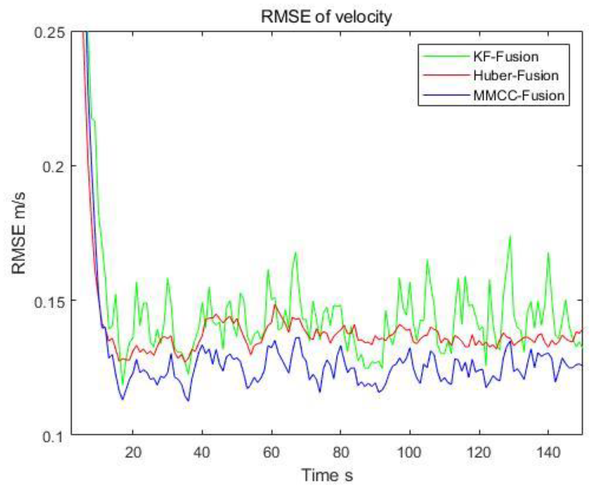
In Figure 9 and Figure 10, the estimation results are shown. It can be seen that the KF-Fusion method performs worst, mainly due to the sensitivity of the MMSE criterion to outliers. The Huber-Fusion method yields better results by mitigating the impact of outliers using a correction function on the measurements. The MMCC-Fusion-IF method outperforms the others as non-Gaussian measurements are suppressed under the MCC criterion.
5. Conclusions
This paper addresses the multi-sensor fusion target tracking problem based on maximum mixture correntropy with the non-Gaussian process and measurement noise using Doppler measurements. A robust fusion filter is developed by maximizing the mixture correntropy-based cost, which contains the high-order statistics of state prediction and measurement error caused by noise. Furthermore, the selection of the kernel width is discussed. Simulations are performed given different non-Gaussian noise, such as outliers and mixture Gaussian noise. Experiments are performed using simulated data and automatic driving software. The results demonstrate the effectiveness of the proposed method.
Author Contributions
C.Y.: conceptualization, investigation, writing—review and editing. S.L.: writing—review and editing. M.L.: methodology, writing—original draft preparation. All authors have read and agreed to the published version of the manuscript.
Funding
This work is jointly supported by National Natural Science Foundation of China (Grant Nos. 61673262 and 61175028), China Postdoctoral Science Foundation(Grant No. 2019M651498).
Conflicts of Interest
The authors declare no conflict of interest.
Appendix A
Derivation of (20) and (21).
Let , and Equation (17) can then be rewritten in a centralized form as:
where .
Change the form of (34) to obtain:
Apply the matrix inversion lemma
with the identifications
and the innovation gain
Then, the posterior covariance can be calculated as follows:
Therefore, the posterior information matrix is:
and the posterior information vector is:
References
- Wu, W.; Jiang, J.; Liu, W.; Feng, X.; Gao, L.; Qin, X. Augmented state gm-phd filter with registration errors for multi-target tracking by doppler radars. Signal Process. 2016, 120, 117–128. [Google Scholar] [CrossRef]
- Zheng, J. Structure and Performance Analysis of Signal Acquisition and Doppler Tracking in LEO Augmented GNSS Receiver. Sensors 2021, 21, 525. [Google Scholar] [CrossRef] [PubMed]
- Ristic, B.; Farina, A. Joint detection and tracking using multi-static doppler-shift measurements. In Proceedings of the International Conference on Acoustics, Speech and Signal Processing (ICASSP) 2012, Kyoto, Japan, 25–30 March 2012; pp. 3881–3884. [Google Scholar]
- Ristic, B.; Farina, A. Target tracking via multi-static Doppler shifts. IET Radar Sonar Navig. 2013, 7, 508–516. [Google Scholar] [CrossRef]
- Vo, B.T.; Vo, B.N.; Cantoni, A. The Cardinality Balanced Multi-target Multi-Bernoulli Filter and Its Implementations. IEEE Trans. Signal Process. 2009, 57, 409–423. [Google Scholar]
- Karlgaard, C.D. Nonlinear Regression Huber-Kalman Filtering and Fixed-Interval Smoothing. J. Guid. Control Dyn. 2014, 38, 322–330. [Google Scholar] [CrossRef]
- Karlgaard, C.; Schaub, H. Huber-based divided difference filtering. J. Guid. Control Dyn. 2007, 30, 885–891. [Google Scholar] [CrossRef]
- Graham, M.C.; How, J.P.; Gustafson, D.E. Robust state estimation with sparse outliers. J. Guid. Control Dyn. 2015, 38, 1229–1240. [Google Scholar] [CrossRef] [Green Version]
- Principe, J.C. Information Theoretic Learning: Renyi’s Entropy and Kernel Perspectives; Springer: New York, NY, USA, 2010. [Google Scholar]
- Liu, W.; Pokharel, P.P.; Principe, J.C. Correntropy: Properties, and applications in non-Gaussian signal processing. IEEE Trans. Signal Process. 2007, 55, 5286–5298. [Google Scholar] [CrossRef]
- Chen, B.; Liu, X.; Zhao, H. Maximum correntropy Kalman filter. Automatic 2017, 76, 70–77. [Google Scholar] [CrossRef] [Green Version]
- Wang, Y.; Zheng, W.; Sun, S.; Li, L. Robust Information Filter Based on Maximum Correntropy Criterion. J. Guid. Control Dyn. 2016, 39, 1126–1131. [Google Scholar] [CrossRef]
- Chen, B.; Principe, J.C. Maximum correntropy estimation is a smoothed MAP estimation. IEEE Signal Process. Lett. 2012, 19, 491–494. [Google Scholar] [CrossRef]
- Chen, B.; Wang, J.; Zhao, H. Convergence of a Fixed-Point Algorithm under Maximum Correntropy Criterion. IEEE Signal Process. Lett. 2015, 22, 1723–1727. [Google Scholar] [CrossRef]
- Wang, G.Q.; Gao, Z.X.; Zhang, Y.G.; Ma, B. Adaptive maximum correntropy Gaussian filter based on variational Bayes. Sensors 2018, 18, 1960. [Google Scholar] [CrossRef] [PubMed] [Green Version]
- Gan, Q.; Harris, C.J. Comparison of two measurement fusion methods for Kalman-filter-based multisensor data fusion. IEEE Trans. Aerosp. Electron. Syst. 2001, 37, 273–279. [Google Scholar] [CrossRef] [Green Version]
- Wang, G.; Li, N.; Zhang, Y. Maximum correntropy unscented Kalman and information filters for non-Gaussian measurement noise. J. Frankl. Inst. 2017, 354, 8659–8677. [Google Scholar] [CrossRef]
- Udacity’s Self-Driving Car Simulator, Udacity, Mountain View, CA, USA. 2017. Available online: https://github.com/udacity/self-drivingcar-sim (accessed on 2 August 2023).
Figure 1.
Multiple radar fusion scenario using Doppler measurements.

Figure 2.
Algorithm framework.

Figure 3.
Scenario 1.

Figure 4.
Comparison of position estimation performance with complex noise.

Figure 5.
Comparison of position estimation performance with complex noise.

Figure 6.
Position estimation performance with different kernel widths.

Figure 7.
Velocity estimation performance with different kernel widths.

Figure 8.
Scenario 2 of autonomous driving.

Figure 9.
Comparison of position estimation performance with outliers.

Figure 10.
Comparison of velocity estimation performance with outliers.


Table 1.
Fusion estimation RMSE in different non-Gaussian noise.
| Algorithm | Case 1 | Case 2 | Case 3 | Case 4 |
|---|---|---|---|---|
| KF-Fusion | 1.413 | 2.510 | 1.918 | 2.404 |
| Huber-Fusion | 2.165 | 2.050 | 1.907 | 2.226 |
| MMCC-Fusion | 1.555 | 1.753 | 1.725 | 1.890 |
Table 2.
Velocity estimation performance with different kernel widths.
| Algorithm | Kernel Widths | Iteration Num | ||
|---|---|---|---|---|
| MMCC-Fusion-IF | ) | 1.895 | 0.249 | 3.85 |
| ) | 1.840 | 0.234 | 2.98 | |
| ) | 2.164 | 0.306 | 2.36 | |
| KF-Fusion | 2.179 | 0.312 |
Disclaimer/Publisher’s Note: The statements, opinions and data contained in all publications are solely those of the individual author(s) and contributor(s) and not of MDPI and/or the editor(s). MDPI and/or the editor(s) disclaim responsibility for any injury to people or property resulting from any ideas, methods, instructions or products referred to in the content. |
© 2023 by the authors. Licensee MDPI, Basel, Switzerland. This article is an open access article distributed under the terms and conditions of the Creative Commons Attribution (CC BY) license (https://creativecommons.org/licenses/by/4.0/).
Share and Cite
MDPI and ACS Style
Yi, C.; Li, M.; Li, S. Multi-Sensor Fusion Target Tracking Based on Maximum Mixture Correntropy in Non-Gaussian Noise Environments with Doppler Measurements. Information 2023, 14, 461. https://doi.org/10.3390/info14080461
AMA Style
Yi C, Li M, Li S. Multi-Sensor Fusion Target Tracking Based on Maximum Mixture Correntropy in Non-Gaussian Noise Environments with Doppler Measurements. Information. 2023; 14(8):461. https://doi.org/10.3390/info14080461
Chicago/Turabian StyleYi, Changyu, Minzhe Li, and Shuyi Li. 2023. "Multi-Sensor Fusion Target Tracking Based on Maximum Mixture Correntropy in Non-Gaussian Noise Environments with Doppler Measurements" Information 14, no. 8: 461. https://doi.org/10.3390/info14080461
Note that from the first issue of 2016, this journal uses article numbers instead of page numbers. See further details here.