ECO4RUPA: 5G-IoT Inclusive and Intelligent Routing Ecosystem with Low-Cost Air Quality Monitoring

Abstract

The increase and diversity of low-cost air quality (AQ) sensors, as well as their flexibility and low power consumption, offers us the opportunity to integrate them into broad AQ wireless sensor networks, with the aim of enabling real-time monitoring and higher spatial sampling density of pollution in all parts of cities. Considering that the vast majority of the population lives in cities and the increase in respiratory/allergic problems in a large part of the population, it is of great interest to offer services and applications to improve their quality of life by avoiding pollution exposure in their movements in the open air. In the ECO4RUPA project, we focus on this kind of service, proposing an inclusive and intelligent routing ecosystem carried out using a network of low-cost AQ sensors with the support of 5G communications along with official AQ monitoring stations, using spatial interpolation techniques to enhance its spatial resolution. The goal of this service is to calculate healthy walking and/or cycling routes according to the particular citizen’s profile and needs. We provide and analyse the results of the proposed route planner under different scenarios (different timetables, congestion road traffic, and routes) and different user profiles, with a special interest in citizens with asthma and pregnant women, since both have special needs. In summary, our approach can lead to an approximately average reduction in pollution exposure of 17.82% while experiencing an approximately average increase in distance travelled of 9.8%.

1. Introduction

Urbanisation has meant that three-quarters of Europe’s population now lives in cities. Citizens are constantly confronted with levels of air pollution that violate the safe thresholds for human health defined by the World Health Organization (WHO) [1], generally caused by the natural dynamics of the movement of people and the pollution associated with such transport.

According to Eurostat [2], in 2021, there were 369,000 deaths in the EU resulting from diseases of the respiratory system, equivalent to 7.9% of all deaths in the EU-28. The BBC reported [3] that “around 422,000 people died prematurely in European countries in 2018 due to exposure to harmful levels of fine particulate matter PM2.5”. Moreover, the problem is worse if we consider that a large part of the population has or may have some kind of allergy, respiratory, and skin problem [4]. There is an increasing number of allergens that increase allergic problems, asthma, as well as other respiratory and skin problems [5].

In this scenario, wireless sensor networks (WSN) or Internet of Things (IoT) sensor networks for monitoring air quality (AQ) based on low-cost sensors and supported by 5G technologies, together with artificial intelligence (AI) techniques [6,7], along with official AQ monitoring stations, can help citizens in their day-to-day lives by means of a system that looks after their health when they are on the move, especially when they have respiratory and/or allergy problems. These activities are carried out within the ECO4RUPA project.

To this end, the goal of this paper is to propose an inclusive and intelligent routing ecosystem with the objective of calculating healthy routes according to the profile and particular needs of each citizen (which include pathologies and clinical history) in their outdoor movements, assisted by a real-time AQ monitoring network within an IoT paradigm. In case we do not have a specific profile, as a user requirement, we will use a default one that will try to minimize global pollution exposure.

Notice that, at the international level, the air quality is ruled by ISO 11771:2010 [8] and ISO 37122:2019 [9] according to the European Regulation Directive 2008/50/EC [10], which states that cities with more than 2 million inhabitants must have at least one monitoring station for AQ. Thus, this monitoring network is supported by publicly available data from official AQ monitoring stations for polluting gases (the network of stations of the Generalitat Valenciana [11]) as well as other stations managed by the local councils, such as in Valencia city [12]. In Figure 1a, we show an example of an official AQ monitoring station, in particular from Burjassot (outskirts of Valencia, Spain). All this gathered information is also improved with statistical techniques of spatial inference to enhance the spatial resolution of these pollutants over the city maps. In areas with poor official AQ coverage, we deploy additional ECO4RUPA AQ monitoring nodes, as shown in Figure 1b,c with outdoor and indoor versions, respectively.

The AQ index scale is based on the US-EPA 2016 standard and is classified into six categories, given by different ranges and colours, as follows: range [0–50] as good (green), [51–100] as moderate (yellow), [101–150] as unhealthy for sensitive groups (orange), [151–200] as unhealthy (red), [201–300] as very unhealthy (purple), and more than 300 as hazardous (dark red). In Figure 2, we show a map with these official AQ monitoring stations, along with an indicator of the AQ index. In this case, all the different stations were reasonably good by the time they were queried. In Figure 3, we show, at a higher scale, the AQ index for the Valencia community region [13]. It must be stressed that in Figure 3, the pollution is mainly due to ozone, $O_3$, which is a secondary pollutant derived from the combustion of fossil fuels.

The rest of the paper is structured as follows. In Section 2, we show available AQ sensors and the related work. In Section 3, we analyse the different design alternatives to be used in the broad monitoring network and its architecture. In Section 4, we consider the options to integrate and merge the information obtained for the route planner. In Section 5, we present and discuss the results with different users’ profiles. Finally, in Section 6, we summarise the main conclusions and future work.

2. State of the Art

With regard to AQ monitoring, it should be noted that there are three distinct types of monitoring, at least, based on the different types of gases. That is, greenhouse gases (under control by emissions monitoring), chlorofluorinated gases (analysed in the upper layers of the atmosphere), and pollutants, which include nitrogen dioxide ($N{O}_2$), sulfur dioxide ($S{O}_2$), carbon monoxide ($CO$), ozone ($O_3$), as well as benzols and heavy metals (lead ($Pb$), arsenic ($As$), and cadmium ($Cd$)). From these areas, the most relevant for citizens is the last one, the pollutants, most of which come from the combustion of fossil fuels in the city and for which there are regulations and standards for their control, such as Directive 2008/50/EC.

With concern to pollutants, the recent boom in low-cost AQ sensors, due to their ease of installation and low power consumption, makes them increasingly used and interesting to integrate into WSN. These sensors can measure pollutants, such as the ones noted before, as well as volatile organic compounds (VOC, usually measured in totals, TVOC), particulate matter (PM) concentration or particle size distribution, along with temperature (T), atmospheric pressure (AP), and relative humidity (RH). Depending on their operating principle, these sensors are available in different technologies to react to the presence of the pollutant, such as electrochemical, metal oxide semiconductors, photo ionisation detectors, non-dispersive infrared, and light scattering, among others.

Manufacturers also integrate different sensors in the same module, which makes them easier to be used and more attractive. A list of these types of sensors (or sensor modules) and their main characteristics, in particular the type of gases measured as well as the type of data connection, are shown in

Table 1. Examples of different low-cost AQ sensors.

Module	Gas Sensors	Connection Type
SDS011 [17]	PM, T, HR, PA	UART
DL-LP8P [18]	$C{O}_2$, T, HR, PA	LoRAWAN
MiCS-6814 [19]	$CO$, $N{O}_2$, $C_2{H}_{5}OH$, $N{H}_3$, $C{H}_4$	I2C, SPI
ZPHS01B [14]	$PM$, $CO$, $O_3$, $N{O}_2$, TVOC, T, HR	UART

. From all of them, the one we consider to have the best performance, the largest number of gases, and the best quality/price ratio is ZPHS01B [14]. In addition, we can highlight different commercial initiatives [15,16] for AQ monitoring, also considered as low cost, based on a network system that auto-calibrates the AQ measurements.

However, with reference to the measuring ranges and measurement quality of low-cost AQ sensors, the recent CEN/TS 17660-1:2021 [20] standard has set the criteria established by Directive 2008/50/EC for the equivalence of sensor systems used outdoors with the instruments for indicative measurements and objective estimations. In this scenario, these sensors have many limitations as they do not provide a reliable absolute measurement and therefore cannot be used as a substitute for a reliable absolute measurement, nor as a substitute for a reliable reference [21]. In practice, these sensors can be used to provide an order of magnitude and/or awareness of AQ and to allow the identification of pollution hot spots. Nevertheless, to increase the reliability of the readings, the measurements of these sensors can be used as input to the modeling procedure, assisted with AI techniques [6,7] and together with other data, typically measurements of other pollutants and ambient conditions (T and RH).

Furthermore, if we take into account the pollution information in a city, we can plan and influence the calculation of routes for citizens, also known as a route planner, according to the particular citizen’s profile and needs. A route planner is a specialised search algorithm designed to find the optimal way to travel between two or more specific locations, which tries to minimize a determined cost function. In [22], a routing application is introduced that calculates the least polluted route through the streets. The authors employ a modified version of the popular Ant Based Control routing algorithm as the basis for their routing algorithm. To incorporate pollution data and minimize travel time, the authors tackle a multi-parameter problem.

Similarly, in [23], the significant health risks associated with air pollution are emphasized, with AQ being influenced by factors such as time of day, location within the city, and traffic intensity. To forecast AQ over time, the authors devise a meteorological model integrated into the Healthy Urban Route Planner (HURP), specifically designed for cyclists and pedestrians in Amsterdam (Netherlands). HURP enables users to select and plan a route that promotes a healthier environment, utilizing information gathered from various systems. Traffic emissions are computed based on observed traffic intensities and emission factors. The authors utilize the WRF-Chem atmosphere and AQ model, which generates daily forecasts within a 48-h span, providing temperature and pollutant concentration forecast maps. These maps are then transformed into a unique metric that combines both factors. Hourly data of this metric are incorporated into the route planner, which employs the open source routing library pgRouting (pgRouting extends the PostGIS/PostgreSQL geospatial database to provide geospatial routing functionality) to identify healthier routes. Researchers from the National Institute for Public Health and the Environment in the Netherlands (RIVM) have developed the Atlas Living Environment [24]. Utilizing location-specific parameters, they generate maps displaying the local environment, particularly focusing on $PM10$, $PM2.5$, $N{O}_2$, and $O_3$ densities. These maps are derived from real-time measurements and prediction models. Additionally, the authors have developed an application that forecasts the AQ index for the next 48 h.

Along these lines, in [25], a monitoring system is introduced that utilizes a mobile network implemented on Android devices to provide real-time air pollution information to users. The pollution data collected from various sources are stored on a cloud-based server, facilitating real-time analysis and the development of an air pollution model. To measure air pollution levels, eco-sensors are deployed on public transport systems or bicycles. However, low-end sensors often suffer from reduced accuracy compared to more advanced sensors, as noted above. In [26], a system for air pollution monitoring in Mauritius Island is shown, featuring a novel data aggregation algorithm specifically designed for air pollution monitoring systems. In [27], a dynamic routing was carried out using data from a set of pollutant particles of particulate pollutants considered PM 10. The researchers used an open source routing machine (OSRM) to perform the routing. Finally, in [28], the authors also explore the integration of air pollution data with route planning. However, they propose alternative planning algorithms that aim to distribute traffic more evenly across urban areas. The authors demonstrate that such algorithms not only help alleviate traffic congestion but also contribute to reducing overall air pollution levels in urban environments.

Other alternatives to find out trajectories and routes are shown in [29,30]. However, our goal is slightly different, as we focus on minimizing pollution exposure against other criteria.

We can highlight several commercial applications known as route planners, such as Google maps [31], Ants Route [32], and Here [33], to name a few. Nevertheless, we must stress that these applications are focused mainly on driving and based on the shortest distance.

In summary from the related work, we can see that there are several initiatives to improve mobility and route planners with different strategies, but these are not focused on the user’s profiles and his/her needs for healthy routes. Thus, this is the goal of this paper.

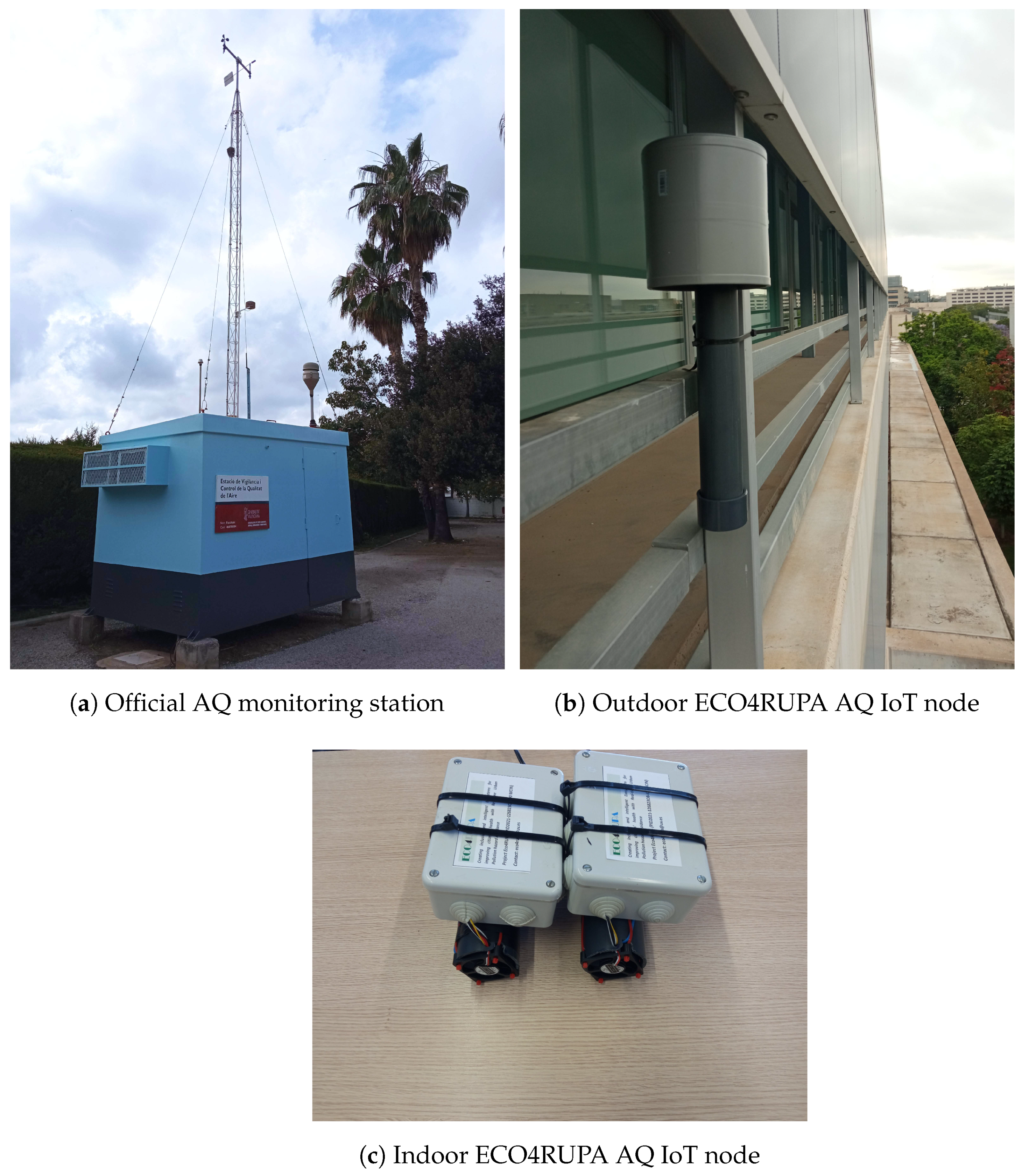
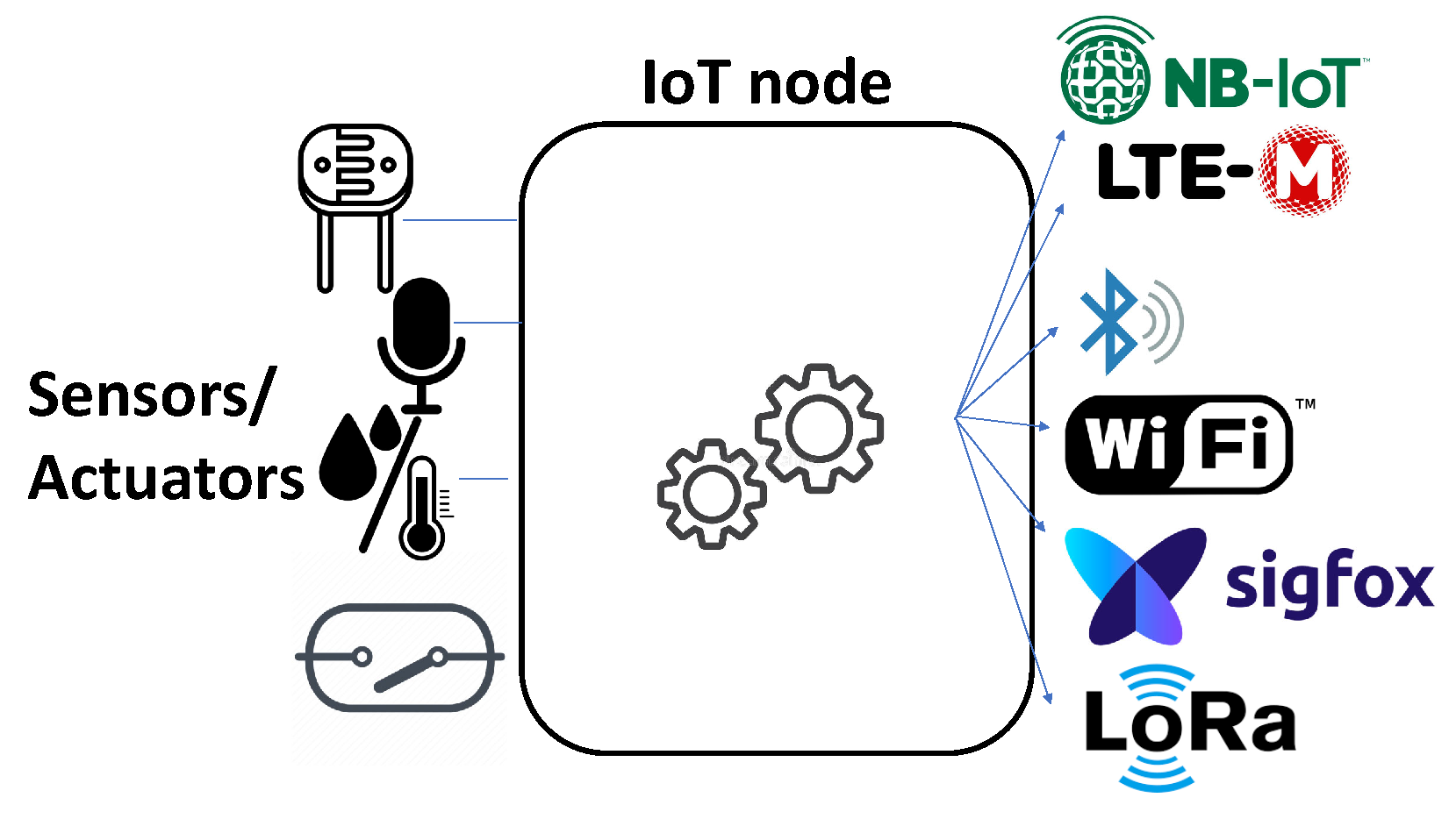
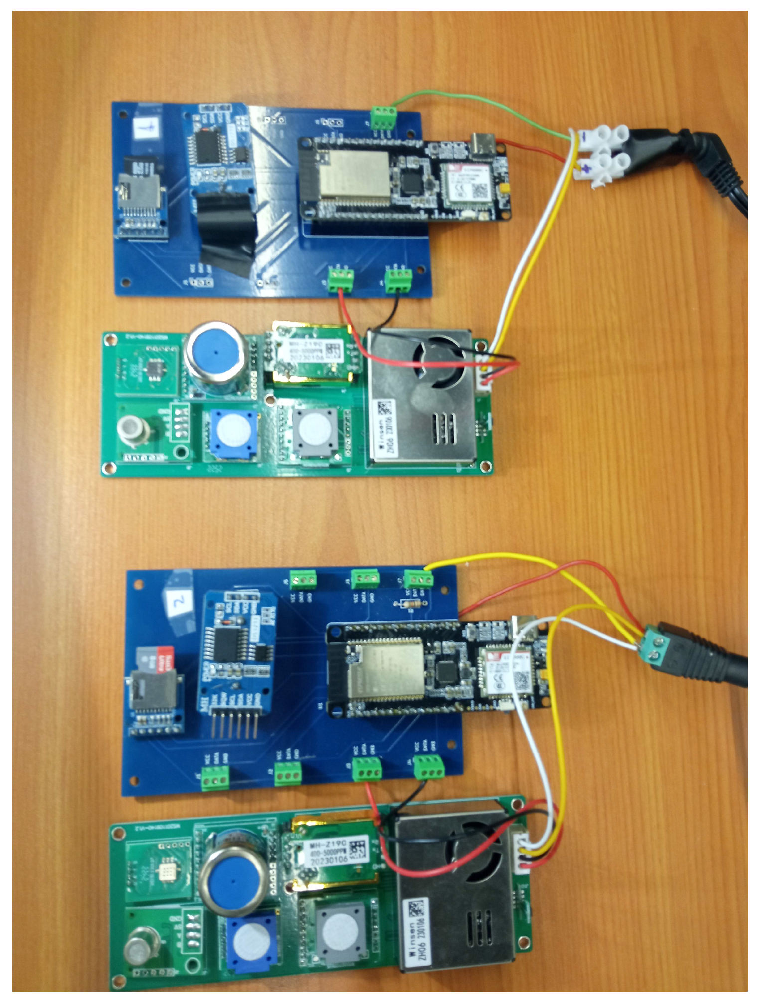
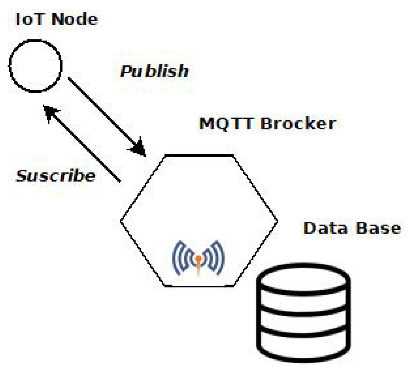
3. Design Alternatives and Techniques for a Broad AQ Monitoring Network and Its Architecture

For this purpose, the first step is to design and build the AQ monitoring network based on low-cost elements, adjusted with official AQ monitoring data. This network will be set up with ECO4RUPA IoT nodes based on a microcontroller that connects to different low-cost AQ sensors, seen in Section 2, with the option of different communication alternatives, as shown in Figure 4.

In case of failure, each IoT node incorporates a real-time clock, a memory card, and a watchdog mechanism for its recovery.

We have initially selected the ESP32 microcontroller [34], due to its performance and quality/price, as it offers in each model the possibility of having different antennas, as well as the possibility to implement different communication standards. The ESP32 is a series of low-cost, low-power system-on-chip microcontrollers that embeds several communication modules. Based on this microcontroller, it is worth noting the Pycom (Pycom Ltd. went into bankruptcy in September 2022, but the newly created Pycom BV took over the company) FiPy module [35] includes technologies such as Lora/Sigfox, WiFi, and Bluetooth, and cellular technologies such as long term evolution (LTE) for machines (LTE-M) and narrow band IoT (NB-IoT). Notice that this FiPy module is flexible enough and permits the building of this type of IoT node.

Thus, since our goal is to cover different scenarios in urbanized areas, these ECO4RUPA low-cost AQ monitoring nodes have been designed to be flexible and can integrate all these technologies, as shown in Figure 4. In particular, we use one technology or another based on the available wireless services at the sampling point in the deployment using direct connection, without multihop.

In particular, Figure 5 depicts a hardware prototype of the implemented AQ IoT monitoring node, with the connection of the ESP32 microcontroller to the ZPHS01B AQ sensor module. Figure 1b,c show the indoor case (for tunnels and indoor environments) for this node that includes a tube and a fan to make air flow pass through the sensor board and also the outdoor version, where the air intake is at the bottom of the tube that sucks it in with a small fan. As noted before, these IoT nodes are used as a coarse reference of the AQ, compared with the measurements provided by the official AQ monitoring stations. The direct measurements taken from these low-cost sensors, in order to be considered valid, are processed by AI-based algorithms to correct and adapt the measurements to reliable values [6]. This process is out of the scope of this paper, as we focus only on how to calculate healthy routes according to the particular citizen’s profile and needs.

The communication scheme of the IoT node with the infrastructure is detailed in Figure 6. It is based on the IoT Message Queue Telemetry Transport (MQTT) protocol, which transmits information via messages between the nodes and the MQTT broker. It should be noted that MQTT allows three levels of quality of service (QoS) to verify the delivery of messages and also several security mechanisms regarding the transmitted data. We have chosen the highest QoS level, QoS-2, which guarantees the delivery of messages only once, without loss or duplication. In terms of security, we use username and password-based login, both at the broker and at the clients, and SSL-certified encryption for transmitted data. The data received are stored locally in a database. For the publishing process, nodes can create a new topic by simply publishing to it, so that more nodes can be added to the IoT system, which greatly facilitates the scalability of the system. These data can also be stored in the cloud, providing additional backup and security against data loss. To graphically visualise the data, the geographical positions of the nodes are indicated.

Notice that the placement of these ECO4RUPA low-cost AQ monitoring nodes will improve the coverage given by the official AQ monitoring stations as noted before, following criteria explained in Section 4.2.

4. Data Fusion, Spatial Interpolation, and Route Planner Application

This section describes the core of the healthy router planner. The goal is to calculate healthy walking and/or cycling routes according to the particular citizen’s profile and needs. For the development of this service, its flowchart is shown in Figure 7. In this case, initially, the user launches a request for a route calculation. With this action, his/her user profile is analysed, and based on it, the appropriate variables (specific pollutants) will be considered, and a complete interpolation in the area of interest defined by the search using Kriging technique is performed. Subsequently, these values are superimposed on the geographical map and define the metric to be minimised in the route search.

Notice that the minimum and recommended time frequency used for AQ monitoring is 10 min, according to ISO 11771:2010 [8], ISO 37122:2019 [9], and European Regulation Directive 2008/50/EC. In practice, this time interval is enough to provide accurate pollution information for the route planner, and this time scale is sufficient for this purpose.

4.1. Analysis of the User’s Profile: Weighting Pollutants

Based on the users’ requirements (specified within his/her profile), we estimate the pollution according to it, as a combination of the different parameters (pollutants) by weighting their different measurements in the area of user mobility. In particular, as a proof of concept, we have considered citizens with asthma and pregnant women without a lack of generality. In this case, we will use the following weights for the different pollutants according to the literature.

In the case of asthma, we assign 40% for ozone, $O_3$, ($\mathsf{\mu }\mathrm{g}/{\mathrm{m}}^3$); 10% for $N{O}_2$ ($\mathsf{\mu }\mathrm{g}/{\mathrm{m}}^3$); and 50% for $PM2.5$. These weights are assigned because $PM2.5$ is considered one of the most dangerous pollutants, as it can penetrate the lungs and cause various health problems [36]. Furthermore, $O_3$ is an oxidant known to irritate the airways and has a clearly defined effect on asthma exacerbation [37]. In addition, according to [37,38], the results of a meta-analysis, there is evidence to support the link between increased ozone concentration and $N{O}_2$, which worsens asthma.

In the case of pregnant women, we assign 5% for $O_3$ ($\mathsf{\mu }\mathrm{g}/{\mathrm{m}}^3$), 35% for $N{O}_2$ ($\mathsf{\mu }\mathrm{g}/{\mathrm{m}}^3$), 20% for $PM2.5$, 30% for $CO$ $\mathrm{mg}/{\mathrm{m}}^3$, and 10% for $PM10$. These gases are chosen because, according to [39], exposure to $O_3$, $N{O}_2$, and $CO$ is associated with a reduction in neonatal weight, and exposure to $PM2.5$ and $PM10$ is related to an increased risk of premature birth. In addition, $N{O}_2$ adds delay in the development of children’s attention span, according to a study conducted by [40]. We assign 30% for $CO$ because exposure to this gas can directly affect the fetus through oxygen deficiency [39], which can cause brain damage, developmental delay, and complications during pregnancy [41]. For $PM2.5$ and $PM10$, we assign a weight of 20% for $PM2.5$ and 10% for $PM10$, because they have been associated with complications during pregnancy, such as premature birth, low birth weight, and respiratory problems in the fetus. Finally, we assign only 5% for $O_3$, because we have found studies that say that $O_3$ exposure increases the risk of premature birth, low birth weight, and respiratory problems in the fetus, but others do not confirm this relation [39].

Notice that, in practice, these weights will be personalized based on the end user’s requirements, and they could even be saved within his/her profile. In case we do not have a specific profile, as a user requirement, we will use a default one that will try to minimize global pollution exposure using an equal distribution of weights as noted in Section 1.

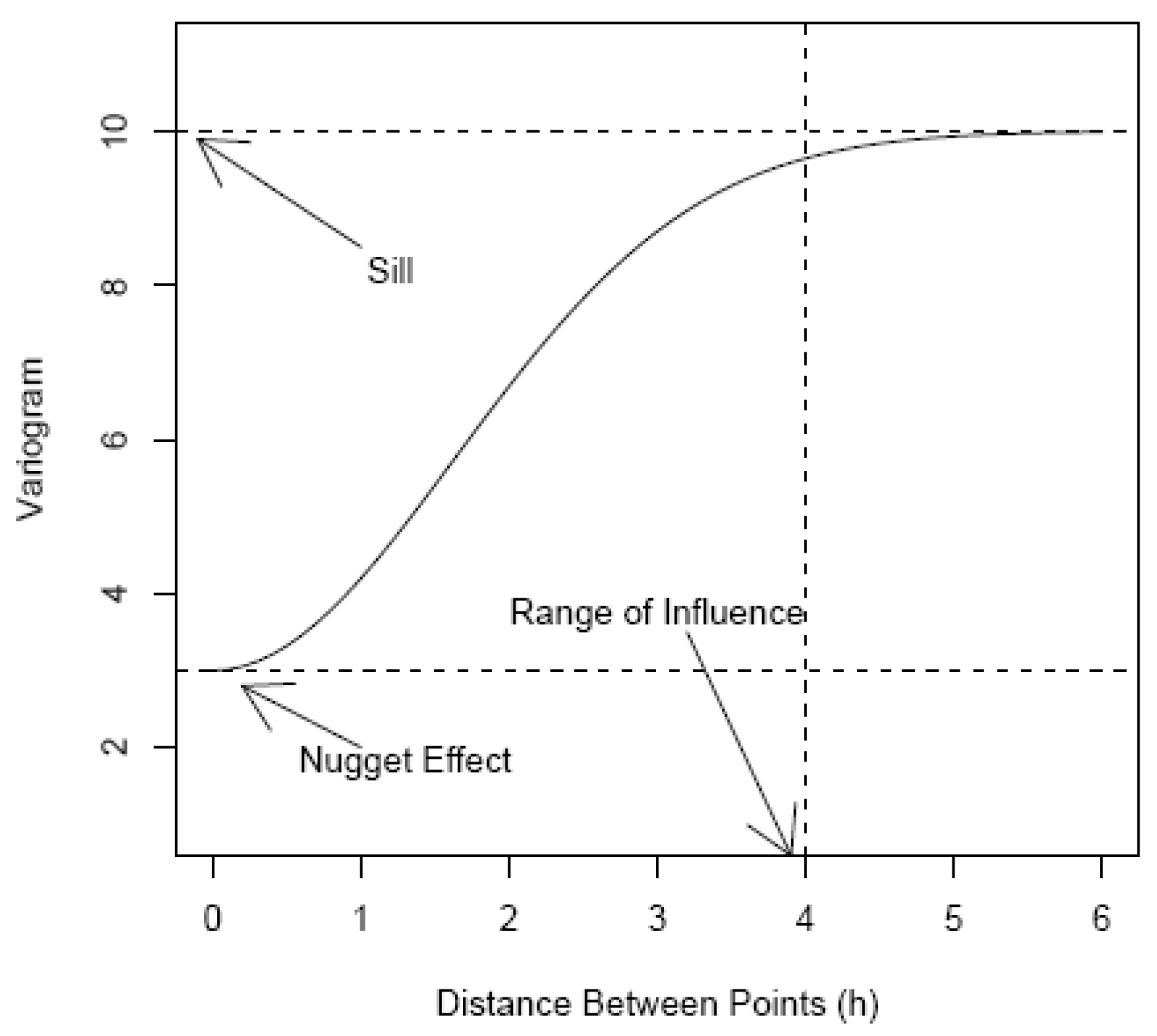
4.2. Kriging for Spatial Interpolation of Pollution

Since the spatial sampling is still limited to the spots where the IoT nodes are deployed and/or the official AQ monitoring stations are installed for a real-time map of the pollutants, a spatial interpolation technique is required, because it is necessary for accurate pollution measurements at the different points over the city map in order to analyse the different paths for the routes.

Kriging [42] is a spatial statistical technique that allows the analysis of geolocated information and is based on spatial autocorrelation, unlike other techniques such as inverse distance weighting (IDW) and splines [42,43]. The main idea with Kriging is that the estimated variable is given by a deterministic (without spatial influence) part and a random (with spatial influence) part. In this case, Kriging employs the spatial function from the random section in order to deliver the best linear unbiased estimator. Thus, the information gathered from the IoT nodes establishes a dataset associated to different locations with their coordinates, longitude, and latitude, as a first step to applying the Kriging technique.

Based on this approach, we are interested in estimating a variable z within a region D in a 2-dimensional map ($D\subset {\mathbb{R}}^2$). For this, we obtain measurements of the variable z at a finite number of points (n points) within the region, denoted as $z\left(s_1\right),z\left(s_2\right),\dots ,z\left(s_n\right)$.

The covariance between measurements $z\left(s_1\right)$ and $z\left(s_2\right)$, denoted as $cov[z\left(s_1\right),z\left(s_2\right)]$, depends only on the difference in locations (distance and direction) between these two points.

In order to characterize the random behavior of the variable being estimated in Kriging, we use the variogram function, which measures how the variable changes with respect to distance. The variogram is defined as $2\gamma (s_1-s_2)=E\left[{(z\left(s_1\right)-z\left(s_2\right))}^2\right]$ and the semivariogram is half of the variogram, which can be represented as $\gamma (s_1-s_2)={\sigma }^2-cov[s_1-s_2]$, assuming that the mean $\mu$ and the variance ${\sigma }^2$ are constant across the region, an assumption usually made for geostatistical data. In case of an isotropic process, the variogram can be expressed in terms of an auto-correlation function $\rho$ as $2\gamma \left(h\right)=2{\sigma }^2(1-\rho \left(h\right))$, where h is the separation between two points.

The variogram is a key point in the Kriging technique and it requires three attributes, as depicted in Figure 8. First, the sill, which is the maximum height of the variogram curve, where, at large distances, the correlation between measured values becomes independent. Second, the range, representing the distance beyond which pairs of points are negligibly correlated. Finally, the nugget effect, indicating a non-zero value at zero distance due to measurement error and micro-scale variation.

Thus, based on the measurements (samples) with the n points within the region D, we will first estimate the empirical variogram and then fit a model to it. For this process, we can locate and improve the placement of the samples (even extra samples) using the ECO4RUPA AQ monitoring nodes, in order to enhance this variogram if it were necessary. Common models include spherical, exponential, Gaussian, and power models [43]. The variogram model will allow us to estimate values at unmeasured locations.

Next, linear interpolation is used to estimate the value $\widehat{z}\left(s_0\right)$ at a location $s_0$ based on these n measurements $z={[z\left(s_1\right),\dots ,z\left(s_n\right)]}^T={[z_1,\dots ,z_n]}^T$ given by ${\widehat{z}}_0=w_0+{\sum }_1^N{w}_i{z}_i=w_0+w^{T}z$. For this estimation, we calculate the different weights $w_i$ that minimize the estimation variance, which is derived from the input variogram model. There are different types of Kriging, such as simple Kriging (SK) and ordinary Kriging (OK), differing mainly in the treatment of the mean value of the stochastic field. Simple Kriging assumes the mean value $\mu$ is known and constant, whereas ordinary Kriging considers it unknown and constant, providing a more realistic approach to the estimation process.

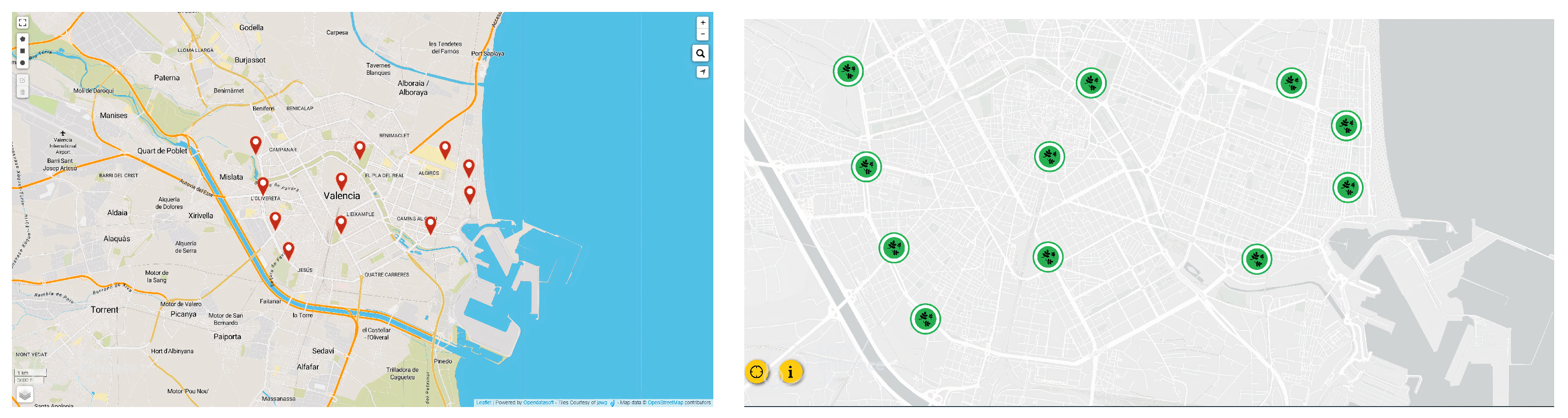
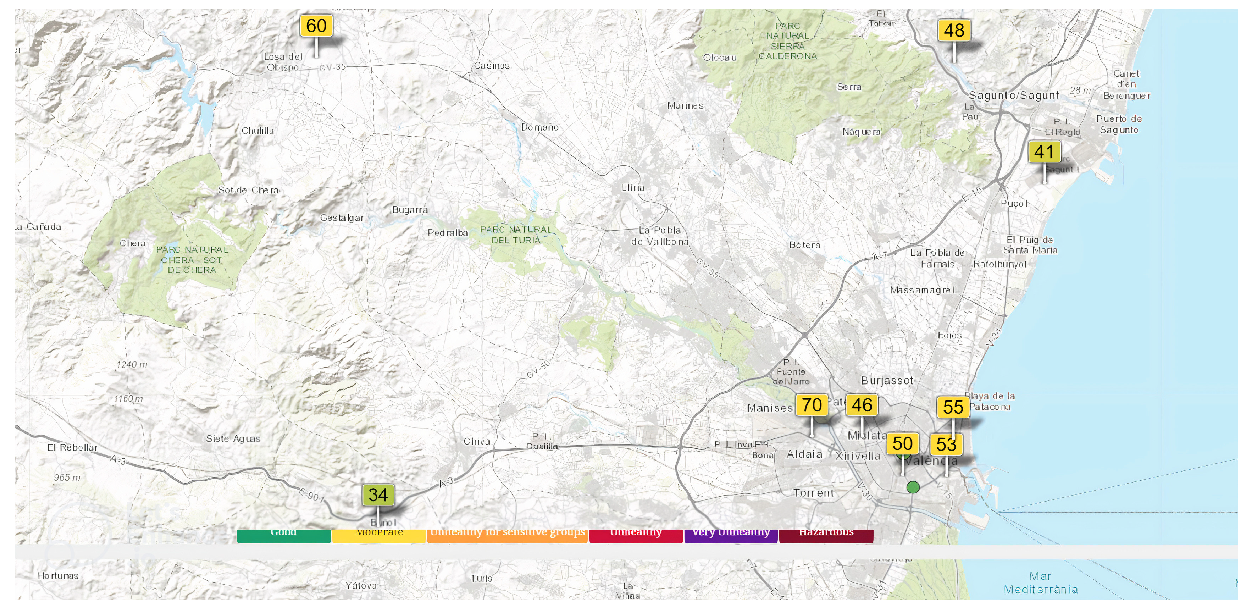
4.3. Mapping of Pollution over the Grid on the City

Once we define the pollution for each user and it has been interpolated with OK over the city map on the area of the user mobility, we need to map this pollution over the grid of the city.

For this, the street network within a city is represented as a bidirectional graph, where nodes correspond to intersections and edges represent street segments. Each edge is associated with a parameter that signifies the cost of travelling along that particular segment. Common routing algorithms aim to minimize the total cost of a route by considering the cumulative costs along the edges, known as the cost function, in this case, given by the exposure to pollution for each user.

Notice that to do this, we have to assign the pollution at each point over the city map by using a grid of 0.0001 decimal degrees that each correspond to 11.5 m (since 360º corresponds to the whole perimeter, 40,075 km, of Earth). It is necessary to find the match between each graph node and its corresponding grid point and then assign the pollution value of the grid point to a new attribute of the graph node. In particular, the grid dataframe index is defined as a combination of the longitude and latitude coordinates, and a search over the grid for the corresponding point uses these coordinates as indices.

For this, we have used OpenStreetMap (OSM) [44], which is a collaborative project for the creation of editable and free maps. We can find different libraries and tools such as OSMnx [45] for Python, which will allow us to analyse these maps in a coherent way.

It is worth emphasizing that Krigring could be seen as a way to gather an accurate measurement of a concrete position in the map, but it is also true that it is not considering the altitude of the available buildings and objects available in the urban landscape. Thus, even if it is technically possible, the authors have decided to limit the concrete geographical positions where the Kriging algorithm is applied to the geographical locations of the nodes of the graph associated to the map of the city. Such nodes are, by definition, intersections/joints, i.e., roads. Thus, the fact that we are only using the technique in such nodes makes the calculation really accurate, as the altitude along the edges and nodes of the road is very constant and linearly incremental, where the change in altitude per every 100 m rarely is higher than 5% in urban areas.

Once the pollution values have been assigned to the nodes of the graph, the next step is to assign weights to the edges of the graph to convert it into a weighted graph. To determine the weights of the edges, the criterion based on the weighted average between the nodes that connect each edge will be used, considering both the pollution values registered at that specific time and the distance between the nodes. This means that the weight of an edge will be the average of the pollution measurement values of the nodes connecting that edge, multiplied by the distance between the two nodes. This is because the travel time between two nodes is assumed to be directly proportional to the distance. In addition, the pollution to which people are exposed is proportional to the exposure time. Therefore, the pollution value and the length of the street segment are multiplied to obtain the cost function.

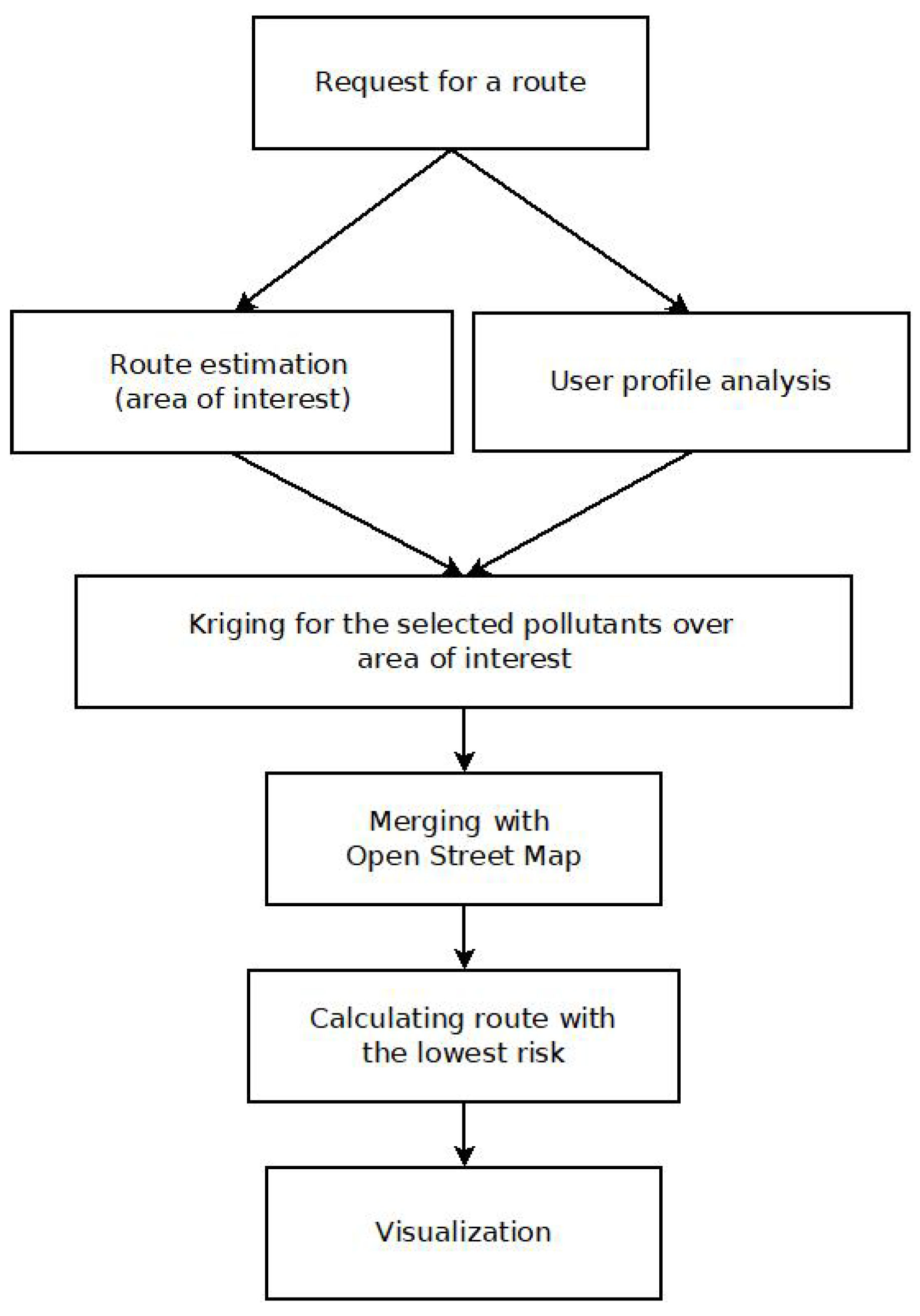
4.4. Healthy Route Planner

With the weighted graph in the area of user mobility with the pollution weights of the edges, we can proceed to find the path that minimizes overall exposure to pollution.

To do this, we identify the node closest to our departure location and the node closest to our arrival location. The widely used Dijkstra algorithm (or shortest path first) utilises the edge lengths as the cost function. Then, using the functions provided by the OSMnx library, we construct the optimal route to reach the destination.

5. Results and Discussion

In this section, we provide and analyse the results of the proposed route planner under different scenarios (different timetables, congestion road traffic, and routes) and different user profiles, with a special interest on citizens with asthma and pregnant women, as both have special needs based on the weights defined in Section 4.1.

In particular, the area under test where we have carried out our experiments is Burjassot city (Valencia, Spain), where we have six official AQ monitoring stations nearby (as shown in Figure 9), within a distance less than 5 km. According to the rules and standards noted in Section 1, it was not necessary to install any extra AQ monitoring node. Specifically, our target for the router planner is given by a minimum threshold of 15% of pollution reduction (PR) with an increase in distance (ID) traveled of less than or equal to 10%.

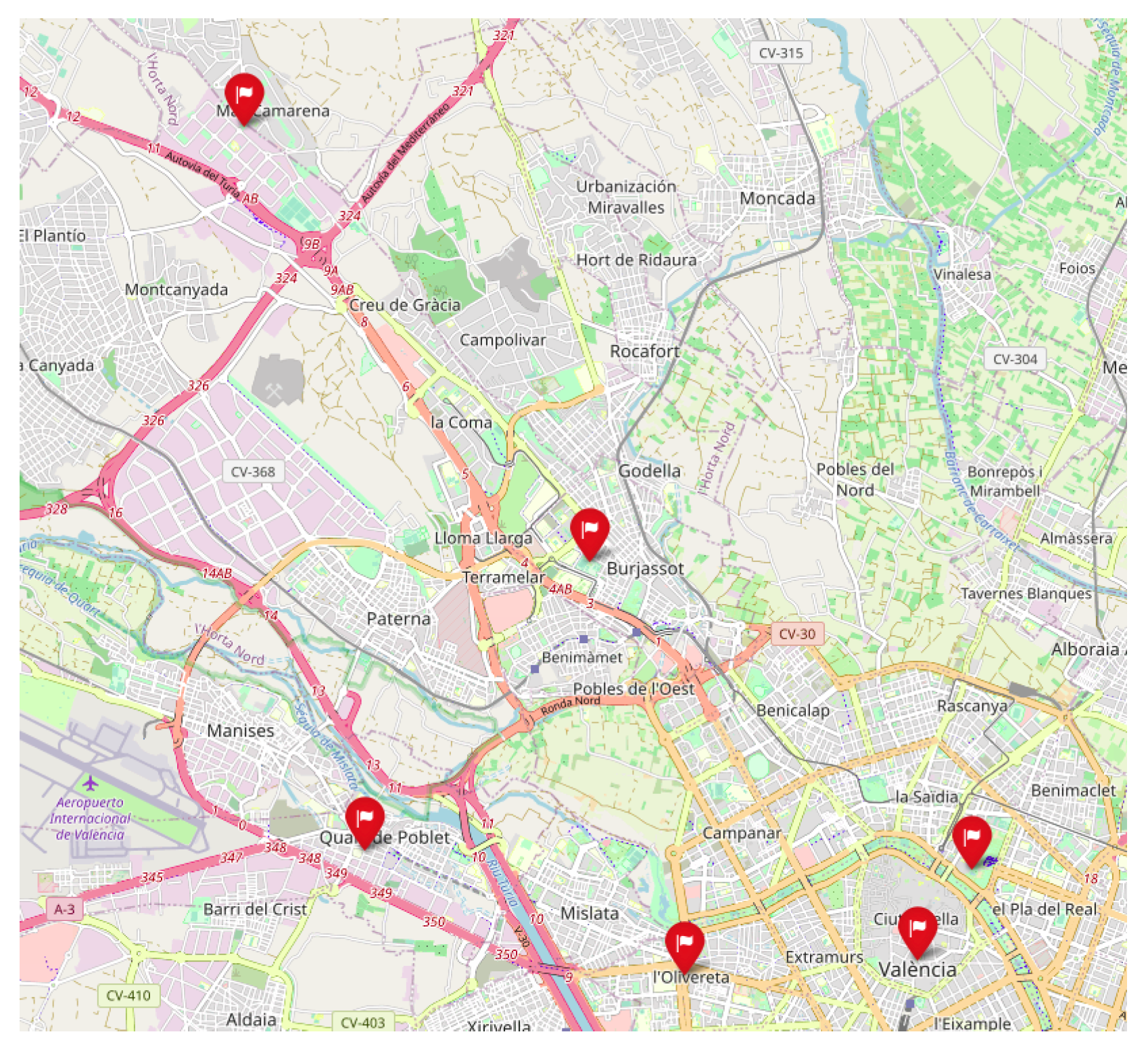
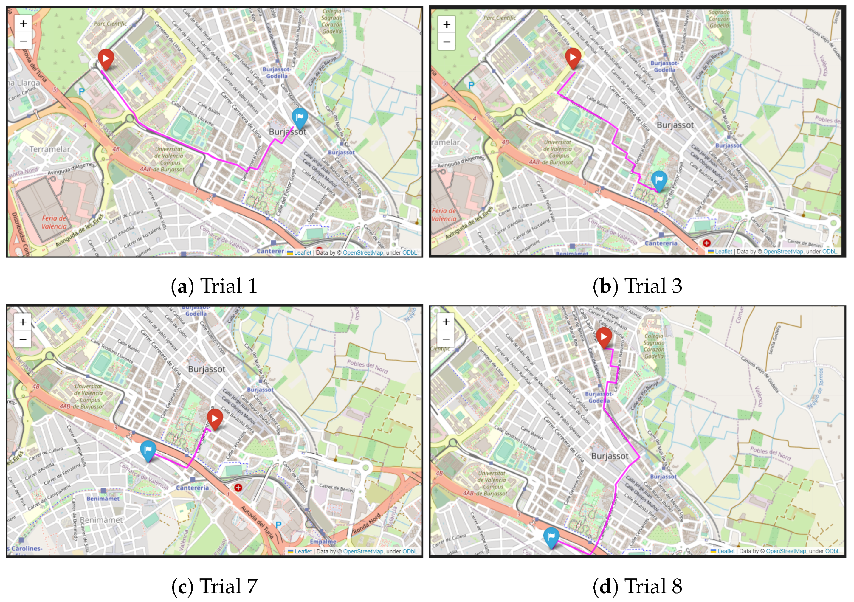
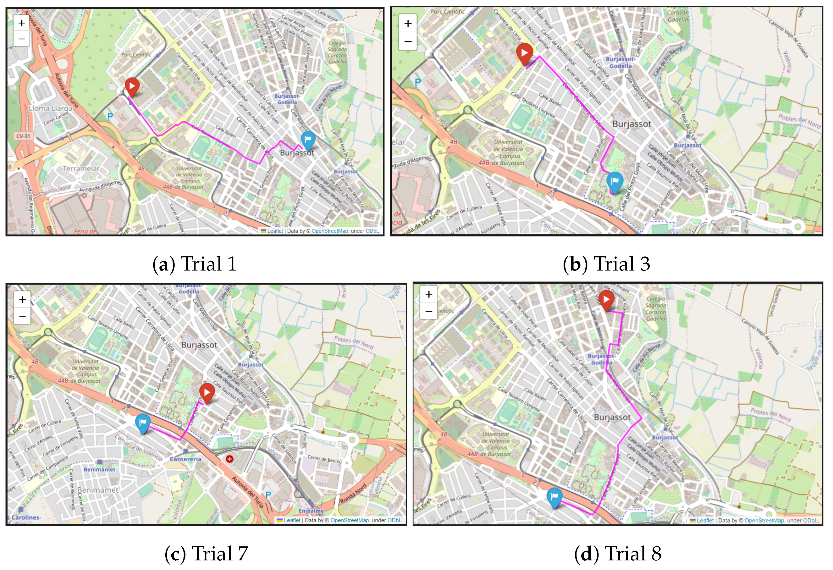
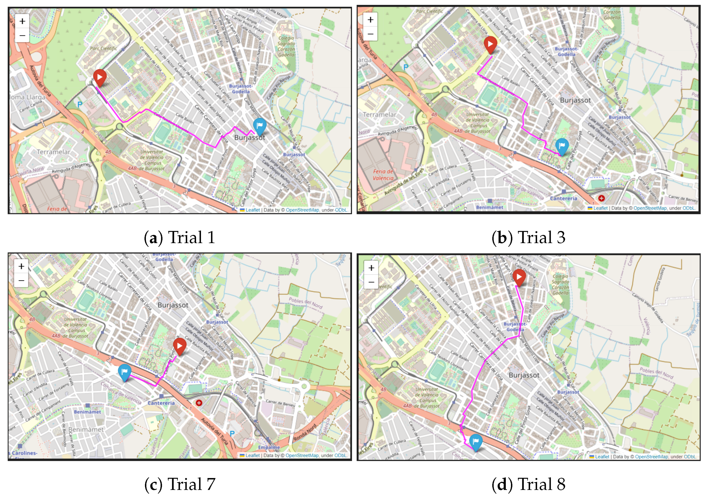
5.1. Analysis of the Healthy Route Planner with Different Scenarios

Figure 10, Figure 11 and Figure 12 show the resulting routes for users with asthma, pregnant women, and shortest path first, respectively.

Table 2. Trials 1–20: detail. In bold are the ones plotted in Figure 10, Figure 11 and Figure 12.

Trial	Src.	Dto.	DD	HH	C. Asthma	D. Asthma	C. Preg.	D. Preg.	C. SPF Asthma	C. SPF Preg.	D. SPF
1	ETSE	Oficina de correos de Burjassot	Friday 16 June 2023	10:13	42,848.7	1728.1	17,927.14	1671.05	43,609.68	17,927.14	1671.05
2	ETSE	Residencia micampus Burjassot	Friday 16 June 2023	12:21	28,349.79	816.02	7679.55	816.02	28,349.79	7679.55	816.02
3	Residencia micampus Burjassot	Parque de la Granja	Friday 16 June 2023	19:32	46,232.2	1295.79	9822.41	1279.08	47,273.17	10,000.21	1278.33
4	C/Vista Alegre 2	Polideportivo de Burjassot	Saturday 17 June 2023	9:21	432.97	850.25	191.17	850.25	492.98	216.3	740.34
5	C/Vista Alegre 2	Hospital IMED	Saturday 17 June 2023	20:47	1290.39	2385.04	322.92	2385.04	1716.59	424.17	2124.88
6	C/Maestro Giner 32	Restaurante Colonial buffet	Sunday 18 June 2023	14:09	954.03	1215.45	323.4	1178.19	1058.74	361.32	1134.74
7	C/Maestro Giner 32	Restaurante Quitin	Sunday 18 June 2023	14:28	413.58	640.03	86.99	640.03	524.55	111.02	627.55
8	C/Vista Alegre 2	Restaurante Quitin	Sunday 18 June 2023	14:31	1161.19	1996.87	249.01	1997.02	1502.93	327.74	1702.75
9	C/Vista Alegre 2	ETSE	Monday 19 June 2023	10:35	415.82	2281.57	893.67	2281.57	778.73	1675.34	1648.43
10	ETSE	Residencia micampus Burjassot	Friday 16 June 2023	12:21	28,349.79	816.02	7679.55	816.02	28,349.79	7679.55	816.02
11	ETSE	C/Maestro Giner 32	Monday 19 June 2023	14:31	546.89	1928.15	156.95	1928.15	624.33	175.94	1928.15
12	C/Vista Alegre 2	Consum 1	Wednesday 21 June 2023	9:32	433.32	850.26	139.79	850.41	493.63	157.11	740.34
13	C/Vista Alegre 2	Consum 2	Wednesday 21 June 2023	9:41	513.38	663.54	159.03	923.98	671.82	159.03	575.77
14	C/Vista Alegre 2	Mercadona	Wednesday 21 June 2023	9:47	341.57	473.96	104.97	494.65	501.38	144.4	470.17
15	C/Lauri Volpi 12	Druni	Wednesday 21 June 2023	11:08	522.42	867.41	154.86	867.41	589.62	168.88	793.06
16	C/Lauri Volpi 15	Mercadona	Wednesday 21 June 2023	12:47	412.1	379.06	110.94	420.58	541.36	134.31	351.59
17	C/Vista Alegre 2	Mercadona	Thursday 22 June 2023	12:32	376.14	473.8	97.69	473.96	570.79	134.76	470.17
18	Parada Burjassot-Godella	Centro de salud	Thursday 22 June 2023	12:48	811.98	1380.04	196.48	1503.31	961.48	233.37	1273.13
19	C/Vista Alegre 2	Parque de la granja	Sunday 25 June 2023	17:19	373.1	528.61	65.95	528.77	551.04	96	502.75
20	C/Maestro Giner 32	Mercado	Monday 26 June 2023	11:46	291.5	666.91	69.12	666.91	381.59	90.15	653.92

depicts the detail for each trial, in bold are the ones plotted in Figure 10, Figure 11 and Figure 12. In this table, each column identifies the trial number, source (src.), destination (dto.), day (DD), hour (HH), total cost with asthma (C. Asthma), total distance with asthma (D. Asthma), total cost for pregnancy (C. Preg.), total distance for pregnancy (D. Preg.), cost with shortest path first (SPF) assuming asthma (C. SPF Asthma), cost with shortest path first assuming pregnancy (C. SPF Preg.), and, finally, distance with SPF (D. SPF).

It is important to highlight that the difference between the optimal healthy route and the shortest route is highly dependent on the selected origin and destination. In some cases, the difference between the shortest route and the optimal healthy route is minimal, for example, in trial number 3 in Table 2. In other cases, there may be a significant difference, for example, in trial number 9 in the same table. Furthermore, the results suggest that there is a trade-off between reduced pollution exposure and journey length.

5.2. Statistical Analysis for the Different Scenarios

We will estimate the average pollution reduction (PR) percentages for each of the trials.

Table 3. Percentage of pollution reduction (PR) and increased distance (ID) for each scenario. In bold are the trials plotted in Figure 10, Figure 11 and Figure 12 and the average.

Trial	% PR with Asthma	% ID with Asthma	% PR with Pregnancy	% ID with Pregnancy
1	1.75%	3.3%	0%	0%
2	0%	0%	0%	0%
3	2.20%	1.35%	1.78%	0.06%
4	12.17%	12.93%	11.62%	12.93%
5	24.83%	10.91%	23.87%	10.91%
6	9.89%	6.64%	10.49%	3.69%
7	21.15%	1.95%	21.65%	1.95%
8	22.74%	14.73%	24.02%	14.74%
9	46.6%	27.75%	46.66%	27.75%
10	12.15%	24.13%	6.39%	24.13%
11	12.4%	15.25%	10.8%	15.25%
12	12.22%	12.93%	11.03%	12.94%
13	23.58%	13.23%	18.6%	37.68%
14	31.84%	0.8%	27.32%	4.95%
15	11.4%	8.57%	8.3%	8.57%
16	23.88%	7.25%	17.4%	16.4%
17	34.1%	0.77%	27.51%	0.8%
18	15.55%	7.75%	15.81%	15.31%
19	32.29%	4.89%	31.31%	4.92%
20	23.61%	1.95%	23.33%	1.95%
Avg.	18.72%	9.27%	16.91%	10.32%

shows % of PR and increased distance (ID) for each scenario, and the average (avg.) is shown in the last row. In bold are the trials plotted in Figure 10, Figure 11 and Figure 12.

Our main goal was to recommend optimal routes that ensure low exposure to air pollution during the journey. First, we have evaluated whether the algorithm recommends routes that have low exposure to air pollution compared to routes that recommend the shortest path (which is the one usually chosen). We are interested in determining whether our proposal excels at providing routes that minimise exposure to these types of pollutants. We have also examined whether routes with low exposure to pollution turn out to be longer compared to shorter routes. We are interested in whether, by prioritising health and reducing pollution exposure, there is a trade-off in terms of distance travelled.

With this evaluation, we validate the effectiveness of our algorithm.

By analysing the trials performed, we can confirm that our algorithm succeeds in reducing exposure to polluted air by 18.72% in cases of asthma, which implies an increase of 9.27% in distance travelled. For pregnant women, our algorithm succeeds in reducing exposure to air pollution by 16.91%, increasing the distance travelled by 10.32%. On average, our approach can lead to an approximately average reduction in pollution exposure in Burjassot (Valencia) of 17.82% while experiencing an approximately average increase in distance travelled of 9.8%. Therefore, it is shown that the route planning system achieves the goal of reducing exposure to high air pollution. These results support the effectiveness of the method in providing healthier navigation options among users, without imposing a significant increase in distance. In addition, there is evidence that the optimal route for health is consistent for both the pregnancy and asthma trials.

6. Conclusions and Future Work

In this paper, we have described a healthy route planner application within the activities carried out in the ECO4RUPA project. The goal of this application is to calculate healthy walking and/or cycling routes according to the particular citizen’s profile and needs, in particular when they require specific care in case of respiratory diseases, trying to reduce the exposure to specific air pollutants based on these profiles. We have shown several profiles as use cases, such as citizens with asthma and pregnant women, where each profile defines a set of weights for the different air pollutants that determine the hazardousness of their exposure.

In order to estimate the distribution of the pollutants over the city map grid, we have used ordinary Kriging. Weighting the different pollutants given by the user’s profile over the map, we define a complex metric that is used as a cost function in order to run the shortest path algorithm. From our results, we have achieved on average a reduction in pollution exposure of 17.82% while experiencing an approximately average increase in distance travelled of 9.8%.

Notice that this healthy route planner application uses data from both official static AQ stations (mainly) and the low-cost ECO4RUPA AQ nodes when it is necessary. These ECO4RUPA nodes are simpler and easier to be deployed, but they are less accurate and their raw measurements must be further processed (including calibration) in order to provide accurate AQ monitoring data. In addition, the lifetime of the sensors equipped on these low-cost nodes is shorter, between 6 and 12 months. However, due to their cost, we can replace them when needed, compared with the official stations that require weekly maintenance.

In future work, along the same lines, although it is not a pollutant gas, we could add pollen to this list. Pollen is of great concern to people with allergic pathologies. However, notice that, unlike the polluting gases, pollen is controlled in a more complex way through health institutions using traditional and even legacy systems that require a posteriori analysis of the collection filters, analyzing the different particles one by one. In addition, it must be noticed that there are other alternative and complementary metrics, such as subjective noise annoyance, which can be part of this route planning algorithm [46].

References

1. Adair-Rohani, H. Air Pollution Responsible for 6.7 Million Deaths Every Year. 2023. Available online: https://www.who.int/teams/environment-climate-change-and-health/air-quality-and-health/health-impacts/types-of-pollutants (accessed on 27 February 2023).
2. Eurostat: Statistics Explained. Respiratory Diseases Statistics. 2022. Available online: https://ec.europa.eu/eurostat/statistics-explained/index.php?title=Respiratory_diseases_statistics#Deaths_from_diseases_of_the_respiratory_system (accessed on 22 May 2023).
3. BBC News. Air Pollution News. 2018. Available online: https://www.bbc.co.uk/news/world-europe-46017339 (accessed on 23 May 2023).
4. Molinari, G.; Colombo, G.C.C. Respiratory allergies: A general overview of remedies, delivery systems, and the need to progress. Int. Sch. Res. Allergy 2014, 1, 1–16. [Google Scholar] [CrossRef] [PubMed] [Green Version]
5. González-Díaz, S.; Arias-Cruz, A.; Macouzet-Sánchez, C.; Partida-Ortega, A. Impact of air pollution in respiratory allergic diseases. Med. Univ. 2016, 18, 212–215. [Google Scholar] [CrossRef]
6. Zimmerman, N.; Presto, A.A.; Kumar, S.P.N.; Gu, J.; Hauryliuk, A.; Robinson, E.S.; Robinson, A.L.; Subramanian, R. A machine learning calibration model using random forests to improve sensor performance for lower-cost air quality monitoring. Atmos. Meas. Tech. 2018, 11, 291–313. [Google Scholar] [CrossRef] [Green Version]
7. Yadav, K.; Arora, V.; Kumar, M.; Tripathi, S.N.; Motghare, V.M.; Rajput, K.A. Few-Shot Calibration of Low-Cost Air Pollution (PM2.5) Sensors Using Meta Learning. IEEE Sens. Lett. 2022, 6, 1–4. [Google Scholar] [CrossRef]
8. ISO 11771:2010; Air Quality -Determination of Time-Averaged Mass Emissions and Emission Factors—General Approach. Technical Report; ISO: Geneva, Switzerland, 2010.
9. ISO 37122:2019; Sustainable Cities and Communities—Indicators for Smart Cities. TC268 Sustainable Cities and Communities. Technical Report; ISO: Geneva, Switzerland, 2019.
10. FAO. Directive 2008/50/EC of the European Parliament and of the Council of the European Parliament and of the Council of 21 May 2008 on Ambient Air Quality and Cleaner Air for Europe. Off. J. Eur. Commun. 2008, L 152, 1–44. [Google Scholar]
11. Conselleria d’Agricultura, Desenvolupament Rural, Emergència Climàtica i Transició Ecològica. Red Valenciana de Vigilancia y Control de la Contaminación Atmosférica. 2023. Available online: https://agroambient.gva.es/va/web/calidad-ambiental/datos-on-line (accessed on 27 May 2023).
12. Ajuntament de Valencia, Minut a Minut. Estaciones Contaminación Atmosféricas. 2023. Available online: https://valencia.opendatasoft.com/explore/dataset/estacions-contaminacio-atmosferiques-estaciones-contaminacion-atmosfericas/table/ (accessed on 21 May 2023).
13. aqicn.org Project. World Air Quality Index Project. 2023. Available online: https://aqicn.org/ (accessed on 27 February 2023).
14. Winsen, Ltd. Air Quality Sensor zphs01b. 2023. Available online: https://www.winsen-sensor.com/d/files/zphs01b-english-version1_1-20200713.pdf (accessed on 20 March 2023).
15. Kunak Tech., Calidad del Aire Urbano: Información Ambiental y Parámetros meteorológicos en Entornos Urbanos. 2023. Available online: https://www.kunak.es/ (accessed on 28 February 2023).
16. Oizom, Ltd. Accurate and Affordable Air Quality Monitoring Solutions. 2023. Available online: https://oizom.com (accessed on 28 February 2023).
17. Nova Fitness Co., Ltd. Air Quality Sensor SDS011. 2023. Available online: https://cdn-reichelt.de/documents/datenblatt/X200/SDS011-DATASHEET.pdf (accessed on 27 April 2023).
18. DecentLab, Ltd. Air Quality Sensor DL-LP8P. 2023. Available online: https://www.catsensors.com/media/Decentlab/Productos/Decentlab-DL-LP8P-datasheet.pdf (accessed on 27 April 2023).
19. SGX, SensorTech. Air Quality Sensor MiCS-6814. 2023. Available online: https://www.sgxsensortech.com/content/uploads/2015/02/1143_Datasheet-MiCS-6814-rev-8.pdf (accessed on 21 May 2023).
20. CEN, CEN/TS 17660-1 Air Quality—Performance Evaluation of air Quality Sensor Systems—Part 1: Gaseous Pollutants in Ambient Air. 2021. Available online: https://www.boutique.afnor.org/engb/standard/din-cen-ts-176601/air-quality-performance-evaluation-of-air-quality-sensor-systemspart-1-gas/eu174644/322334 (accessed on 2 August 2023).
21. García, M.R.; Spinazzé, A.; Branco, P.T.; Borghi, F.; Villena, G.; Cattaneo, A.; Gilio, A.D.; Mihucz, V.G.; Álvarez, E.G.; Lopes, S.I.; et al. Review of low-cost sensors for indoor air quality: Features and applications. Appl. Spectrosc. Rev. 2022, 57, 747–779. [Google Scholar] [CrossRef]
22. Rothkrantz, L. Multi parameter routing in air polluted urban areas. In Proceedings of the 2020 Smart City Symposium Prague (SCSP), Prague, Czech Republic, 25 June 2020; pp. 1–6. [Google Scholar] [CrossRef]
23. Steeneveld, G.; Vreugdenhil, L.; van der Molen, M.; Ligtenberg, A. Towards a Healthy Urban Route Planner for cyclists and pedestrians in Amsterdam. In Proceedings of the Annual Meeting European Meteorological Society, Dublin, Ireland, 4–8 September 2017. EMS2017-305. [Google Scholar]
24. RIVM Institute. Environmental Health Atlas—Explore and Discover Your Living Environment. 2023. Available online: https://www.atlasleefomgeving.nl/en (accessed on 27 May 2023).
25. Alvear, O.; Zamora, W.; Calafate, C.T.; Cano, J.C.; Manzoni, P. EcoSensor: Monitoring environmental pollution using mobile sensors. In Proceedings of the 2016 IEEE 17th International Symposium on A World of Wireless, Mobile and Multimedia Networks (WoWMoM), Coimbra, Portugal, 21–24 June 2016; pp. 1–6. [Google Scholar] [CrossRef]
26. Khedo, K.; Rajiv, P.; Avinash, M. A Wireless Sensor Network Air Pollution Monitoring System. Int. J. Wirel. Mob. Netw. 2010, 2, 31–45. [Google Scholar] [CrossRef]
27. Müller, S.; Voisard, A. Air Quality Adjusted Routing for Cyclists and Pedestrians. In Proceedings of the 1st ACM SIGSPATIAL International Workshop on the Use of GIS in Emergency Management (EM-GIS ’15), Bellevue, WA, USA, 3–6 November 2015; Association for Computing Machinery: New York, NY, USA, 2015. EM-GIS ’15. [Google Scholar] [CrossRef]
28. Vamshi, B.; Prasad, R.V. Dynamic route planning framework for minimal air pollution exposure in urban road transportation systems. In Proceedings of the 2018 IEEE 4th World Forum on Internet of Things (WF-IoT), Singapore, 5–8 February 2018; pp. 540–545. [Google Scholar] [CrossRef]
29. Wang, C.; Li, C.; Qin, C.; Wang, W.; Li, X. Maximizing spatial–temporal coverage in mobile crowd-sensing based on public transports with predictable trajectory. Int. J. Distrib. Sens. Netw. 2018, 14, 1–10. [Google Scholar] [CrossRef]
30. Wu, C.; Liu, Z.; Liu, F.; Yoshinaga, T.; Ji, Y.; Li, J. Collaborative Learning of Communication Routes in Edge-Enabled Multi-Access Vehicular Environment. IEEE Trans. Cogn. Commun. Netw. 2020, 6, 1155–1165. [Google Scholar] [CrossRef]
31. Google. Google Maps. 2023. Available online: https://google.maps/ (accessed on 27 February 2023).
32. AntsRoute. The Solution for Planning Last-Mile Route of Field Workforce. 2023. Available online: https://antsroute.com/en (accessed on 27 February 2023).
33. Here. Our Mission Is to Enable a Digital Representation of Reality to Radically Improve the Way the World Moves, Lives and Interacts. 2023. Available online: https://www.here.com/ (accessed on 27 February 2023).
34. Espressif Systems. ESP32 System-on-Chip. 2023. Available online: https://www.espressif.com/en/products/socs/esp32 (accessed on 28 January 2023).
35. Pycom.io. Fipy, Five Network Development Board for IoT. 2022. Available online: https://pycom.io/product/fipy/ (accessed on 28 December 2022).
36. Kiesewetter, G.; Schoepp, W.; Heyes, C.; Amann, M. Modelling PM2.5 impact indicators in Europe: Health effects and legal compliance. Environ. Model. Softw. 2015, 74, 201–211. [Google Scholar] [CrossRef] [Green Version]
37. Ubilla, C.; Yohannessen, K. Contaminación atmosférica efectos en la salud respiratoria en el niño. Rev. Méd. Clín. Condes 2017, 28, 111–118. [Google Scholar] [CrossRef]
38. Orellano, P.; Quaranta, N.; Reynoso, J.; Balbi, B.; Vasquez, J. Effect of outdoor air pollution on asthma exacerbations in children and adults: Systematic review and multilevel meta-analysis. PLoS ONE 2017, 12, e0174050. [Google Scholar] [CrossRef] [PubMed]
39. Vargas, S.; Onatra, W.; Osorno, L.; Páez, E.; Sáenz, O. Contaminación atmosférica y efectos respiratorios en niños, en mujeres embarazadas y en adultos mayores. Rev. UDCA Actual. Divulg. Científica 2008, 11, 31–45. [Google Scholar]
40. Bienestar, O. La Exposición Al Dióxido de Nitrógeno Durante El Embarazo perjudica La Capacidad de Atención de los Niños. 2017. Available online: https://www.atresmedia.com/objetivo-bienestar/actualidad/exposicion-dioxido-nitrogeno-embarazo-perjudica-capacidad-atencion-ninos_20170803598433970cf2c0f4136d712c.html (accessed on 15 June 2023).
41. ISGlobal. La Exposición a la Contaminación Atmosférica Durante el Embarazo También Perjudica a la Capacidad de Atención en la Infancia. 2017. Available online: http://bit.ly/exposicion-a-contaminacion-atmosferica-durante-embarazo (accessed on 15 June 2023).
42. Isaaks, E.H.; Srivastava, R.M. An Introduction to Applied Geostatistics; Oxford University Press: New York, NY, USA, 1989. [Google Scholar]
43. Cressie, N. Statistics for Spatial Data; John Wiley: New York, NY, USA, 1993. [Google Scholar]
44. OSM Contributors. Open Street Map. 2023. Available online: https://www.openstreetmap.org/ (accessed on 27 May 2023).
45. Boeing, G. OSMnx: New methods for acquiring, constructing, analyzing, and visualizing complex street networks. Comput. Environ. Urban Syst. 2017, 65, 126–139. [Google Scholar] [CrossRef] [Green Version]
46. Segura-Garcia, J.; Calero, J.M.A.; Pastor-Aparicio, A.; Marco-Alaez, R.; Felici-Castell, S.; Wang, Q. 5G IoT System for Real-Time Psycho-Acoustic Soundscape Monitoring in Smart Cities With Dynamic Computational Offloading to the Edge. IEEE Internet Things J. 2021, 8, 12467–12475. [Google Scholar] [CrossRef]
Figure 1. Example of (a): official air quality (AQ) monitoring station in Burjassot (outskirts of Valencia, Spain) [11], (b): ECO4RUPA outdoor AQ IoT node, and (c): ECO4RUPA indoor AQ IoT node.
Information 14 00445 g001
Figure 2. Official air quality (AQ) monitoring network in Valencia city [12] and surroundings; (a) location of the official AQ monitoring stations; (b) AQ colour index based on US-EPA 2016 standard.
Information 14 00445 g002
Figure 3. Map of the air quality for the Valencia community region [13].
Information 14 00445 g003
Figure 4. Generic IoT node for air quality monitoring and communications schema.
Information 14 00445 g004
Figure 5. Example of two ECO4RUPA IoT nodes with ESP32 microcontroller connected to module ZPHS01B with different air quality sensors [14].
Information 14 00445 g005
Figure 6. Communication scheme of the ECO4RUPA AQ IoT node connection and communications protocol.
Information 14 00445 g006
Figure 7. Flowchart of the user application to request healthy routes.
Information 14 00445 g007
Figure 8. A theoretical Gaussian model of variogram for the Kriging technique.
Information 14 00445 g008
Figure 9. Official AQ monitoring stations near Burjassot city (Valencia, Spain).
Information 14 00445 g009
Figure 10. Examples of several trials with asthma. See route details in Table 2.
Information 14 00445 g010
Figure 11. Examples of several trials with pregnant women. See route details in Table 2.
Information 14 00445 g011
Figure 12. Examples of several trials with shortest path first. See route details in Table 2.
Information 14 00445 g012