Leveraging Satisfiability Modulo Theory Solvers for Verification of Neural Networks in Predictive Maintenance Applications

Abstract

Interest in machine learning and neural networks has increased significantly in recent years. However, their applications are limited in safety-critical domains due to the lack of formal guarantees on their reliability and behavior. This paper shows recent advances in satisfiability modulo theory solvers used in the context of the verification of neural networks with piece-wise linear and transcendental activation functions. An experimental analysis is conducted using neural networks trained on a real-world predictive maintenance dataset. This study contributes to the research on enhancing the safety and reliability of neural networks through formal verification, enabling their deployment in safety-critical domains.

1. Introduction

In the last decade, interest in machine learning (ML) and neural networks (NNs) has grown significantly in both research and industry. Neural networks have shown exceptional capabilities for various tasks in different areas of computer science [1,2]. However, their applications are still somewhat limited with regard to safety and security since there are no formal guarantees regarding their reliability and behavior. Despite the considerable research effort that have been made to understand why neural networks behave in a certain way [3,4,5], their inherent complexity makes it difficult to solve this issue.

Providing formal guarantees on the performance of neural networks [6,7,8,9,10,11,12,13,14,15,16,17,18,19,20], known as verification, or making them compliant with such guarantees [21,22,23,24,25,26,27], known as repair, has proven to be similarly challenging, even when using models with limited complexity and size. Additionally, neural networks have recently been found to be prone to reliability issues known as adversarial perturbations [28], where seemingly insignificant variations in their inputs cause unforeseeable and undesirable changes in their behavior.

In this paper, we investigate how satisfiability modulo theory (SMT) technologies can enable the verification of neural networks that exhibit both piece-wise linear and transcendental activation functions. The inherent non-linearity of these functions presents significant scalability challenges, and our goal is to assess the current progress of these technologies for their application in real-world scenarios. To accomplish this, we evaluate the relevant technologies in the context of predictive maintenance (see, e.g., [29] for recent advancements), with a specific focus on AI-based algorithms utilized in the Intelligent Motion Control under Industry 4.E (IMOCO4.E) project [30].

IMOCO4.E is a Key Digital Technologies Joint Undertaking (KDT JU) project that commenced in September 2021. It brings together 46 partners from 13 countries with the goal of enhancing the intelligence and adaptability of mechatronic systems by pushing them to their limits. This objective will be achieved by leveraging novel sensory information, model-based approaches, artificial intelligence (AI), machine learning (ML), and principles of industrial IoT. The IMOCO4.E project aims to provide vertically distributed edge-to-cloud intelligence for machines, robots, and other human-in-the-loop cyber-physical systems that involve actively controlled moving components. By doing so, it will contribute to shaping the transition of European manufacturing towards Industry 4.0, enabling the perception and management of advanced machinery and robotics.

One of the key deliverables of the project is a reference architecture that will be tested and validated in various use cases and pilots across different industrial domains, including packaging, industrial robotics, healthcare, and semiconductors. As part of the project, significant emphasis is placed on researching new methods and techniques for applying neural networks to predictive maintenance. This research aims to revolutionize the operation of product life-cycle management systems. Neural networks have shown promising results in this context as they can analyze data from diverse sources such as sensors, logs, and other equipment monitoring systems, enabling preemptive maintenance that reduces downtime and extends equipment lifespan. However, the usage of neural networks for predictive maintenance, particularly in safety-critical application domains, may be somewhat limited due to the inherent unexplainability of their behavior. To bridge this gap, the incorporation of formal verification techniques could prove essential.

In the paper, we performed an experimental evaluation of various state-of-the-art SMT solvers. We utilized a set of benchmarks consisting of diverse neural network architectures, non-linear activation functions, and properties to be verified using real sensor data from an electric motor. Our objective was to assess the solvers’ capabilities in terms of verifying networks with these activation functions and to achieve realistic accuracy levels.

The results of our evaluation indicate that solvers currently at the cutting edge, which support transcendent functions, can only verify networks with such activation functions to a limited extent.

The rest of the paper is structured as follows. In Section 2, we introduce some basic concepts and definitions we will use in the rest of the paper. In Section 3, we explain our motivations and we present our encoding for the benchmarks we use in the experimental evaluation. In Section 4, we introduce our experimental setup, provide all the information needed to replicate our experiments, and present our results. In Section 5, we report the related work regarding the formal verification of neural networks and focus on the usage of SMT solvers for this task. Finally, in Section 6 we conclude the paper with some final remarks and we outline some of our future research activities.

2. Preliminaries

2.1. Neural Networks

Neural networks are machine-learning models consisting of interconnected computing units, commonly known as neurons. In principle, these neurons can be connected in many different configurations; however, in this work, we are mainly interested in sequential neural networks. These are neural networks arranged in several sequential layers whose neurons are only connected to the neurons of the immediately previous and following layers. The first and the last layer of the network are called, respectively, the input and output layers.

Computationally, the l-th layer of a sequential neural network can be defined as a function $f_l:{\mathcal{I}}_l\to {\mathcal{O}}_l$, where ${\mathcal{I}}_l$ and ${\mathcal{O}}_l$ represent, respectively, the input and output domain of the function. Similarly, a generic sequential neural network can be defined as a function $\nu :{\mathcal{I}}_1\to {\mathcal{O}}_p$, where ${\mathcal{I}}_1$ and ${\mathcal{O}}_p$ are, respectively, the input (output) domain of both the first (last) layer of the network and of the network as a whole. In particular, the neural network function $\nu$ can be expressed as:

$$\nu \left(x\right)=f_p\left(f_{p-1}(\dots f_1\left(x\right)\dots )\right)$$

(1)

In this paper, we focus mainly on layers whose inputs and outputs consist of vectors of real numbers; therefore, we will usually have ${\mathcal{I}}_l\subseteq {\mathbb{R}}^n$ and ${\mathcal{O}}_l\subseteq {\mathbb{R}}^m$.

The structure defined by the various layers of a neural network, their connections, and their hyper-parameters is commonly known as the network architecture. Obviously, the different kinds of layers that can be used in the architecture of a sequential neural network are myriad, and new ones are continuously developed with the advancement of the state-of-the-art. In this work, we focus on the following small subset of layers and architectures.

2.1.1. Fully Connected Layers

Fully connected layers apply an affine transformation to their input: the corresponding function can be written as:

$$f\left(x\right)=Wx+b$$

(2)

where $x\in {\mathbb{R}}^n$ is the input; $W\in {\mathbb{R}}^{m\times n}$ is the weight matrix; $b\in {\mathbb{R}}^m$ is the bias vector; and m is commonly known as the number of hidden neurons of the layer, which controls the size of its output.

2.1.2. Activation Layers

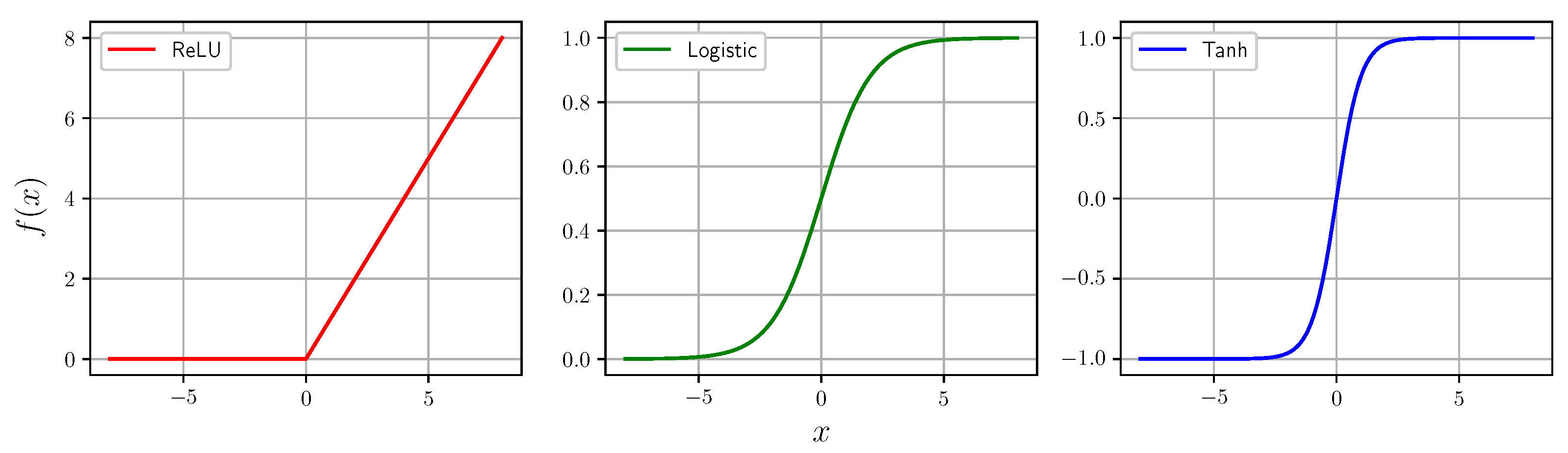
Activation layers apply a particular, usually non-linear, function to each element of the input vector. A general activation function can be represented as $f\left(x\right)=\sigma \left(x\right)$ with $x\in {\mathbb{R}}^n$ and $f\left(x\right)\in {\mathbb{R}}^n$. The neural networks in our experimental evaluation present three different kinds of activation layers: ReLU, Logistic, and Tanh (as shown in Figure 1), whose corresponding activation functions are, respectively,

$$\begin{array}{cc}\hfill f\left(x\right)& =max(0,x)\hfill \end{array}$$

(3)

$$\begin{array}{cc}\hfill f\left(x\right)& =\frac{1}{1+e^{-x}}\hfill \end{array}$$

(4)

$$\begin{array}{cc}\hfill f\left(x\right)& =\frac{e^x-e^{-x}}{e^x+e^{-x}}\hfill \end{array}$$

(5)

Traditionally, the logistic and hyperbolic tangent functions provide the best non-linearity in terms of representativity. However, their computational complexity as transcendent functions is much higher than the one presented by the ReLU, which is piece-wise linear: as a consequence, in state-of-the-art network architectures, ReLU layers are quite common.

It should also be noted that fully connected layers and activation layers are the two most basic components of every neural network: indeed, the first neural networks consisted only of one or more blocks composed of one fully connected layer and one activation layer.

Figure 1. From left to right: the rectified linear unit (ReLU), the logistic, and the hyperbolic tangent activation functions.

Figure 1. From left to right: the rectified linear unit (ReLU), the logistic, and the hyperbolic tangent activation functions.

2.2. Satisfiability Modulo Theory

Satisfiability modulo theories (SMT) is a field of automated reasoning whose aim is to determine the satisfiability of logical formulas by leveraging a combination of decision procedures for various theories. In the early 1980s, researchers recognized that numerous problems in computer science, mathematics, and engineering could be represented as logical formulas containing constraints that belong to different theories such as arithmetic, bit-vectors, arrays, and sets. Traditionally, specialized solvers were used for each theory, but this approach often resulted in inefficient and incomplete solutions. The concept behind SMT was to combine solvers for different theories into a single solver that could handle formulas with mixed theories efficiently and effectively.

SMT solvers are currently widely used in various fields, including software verification, program analysis, optimization, planning, and synthesis. SMT has also played an important role in the development of advanced tools such as theorem provers, model checkers, and symbolic execution engines. In the following, we present the basic syntactic and semantic concepts required to comprehend the rest of the paper.

SMT focuses on the problem of deciding the satisfiability of a first-order formula with respect to some decidable theory $\mathcal{T}$, while an SMT instance is a formula in first-order logic where some function and predicate symbols have additional interpretations. If we consider a first-order formula $\varphi$ in a decidable background theory $\mathcal{T}$, the satisfiability problem consists in deciding whether a model—i.e., an assignment to the free variables in $\varphi$—that satisfies $\varphi$ exists. It should be clear that SMT extends the Boolean satisfiability problem (SAT) by adding background theories such as the theories of real numbers, integers, and data structures. As an example, a formula may contain clauses such as $(x+2\le y)\vee (x>y+z)\vee p\vee q$, where $x,y$, and z are integer variables and p and q are Boolean variables. The predicates involving non-Boolean variables, such as linear inequalities, must be evaluated according to the rules of a corresponding background theory. Some examples of theories of practical interest are the quantifier-free linear integer arithmetic (QF_LIA), where atoms are linear inequalities over integer variables; the quantifier-free non-linear integer arithmetic (QF_NIA), where atoms are polynomial inequalities over integer variables; and the quantifier-free linear real arithmetic (QF_LRA), which is similar to QF_LIA but with real variables.

The satisfiability modulo theories library (SMT-LIB) is a collection of benchmarks and tools designed to support research and development in the area of satisfiability modulo theories. It consists of a set of standardized benchmarks, written in the SMT-LIB language [31], which can be used to evaluate the performance of SMT solvers on various logical formulas with constraints that belong to different theories, such as arithmetic, bit-vectors, arrays, and sets. The SMT-LIB language is a standardized language used for describing logical formulas in the context of satisfiability modulo theories. It is an open and extensible language designed to support a variety of theories and solvers. The language consists of a set of syntactic and semantic rules for specifying logical formulas in various theories.

Current state-of-the-art SMT solvers leverage the integration of an SAT solver and a $\mathcal{T}$-solver, i.e., a decision procedure for the given theory $\mathcal{T}$. To decide the satisfiability of an input formula $\varphi$, the SAT solver enumerates the truth assignments to the Boolean abstraction of $\varphi$, while the $\mathcal{T}$ solver is invoked only when the SAT solver finds a satisfying assignment for the Boolean abstraction to check whether the current Boolean assignment is consistent in the theory. If the assignment is also satisfiable with respect to the theory, then a solution (model) is found for the input formula $\varphi$. Otherwise, the $\mathcal{T}$-solver returns an explanation for the conflict that identifies a reason for the unsatisfiability. Such an explanation is learned by the SAT solver so that it may prune the search tree until either a theory-consistent Boolean assignment is found or no more assignments exist.

For a comprehensive background on SMT, we refer to [32,33].

2.3. Verification

As mentioned in Section 1, the aim of formal verification is to provide formal guarantees about the compliance of a neural network with some specific property of interest. In particular, we focus on input–output specifications: that is, properties defining specific preconditions on the inputs of the neural network and corresponding postconditions that its outputs should respect.

Definition 1.

Given a neural network $\nu :\mathcal{I}\to \mathcal{O}$, a generic input $x\in \mathcal{I}$, and the corresponding output $y\in \mathcal{O}$, we can define an input–output property Φ as a couple $\mathsf{\Phi }=\langle {\varphi }_I\left(x\right),{\varphi }_O\left(y\right)\rangle$, where the precondition ${\varphi }_I\left(x\right)$ and the postcondition ${\varphi }_O\left(y\right)$ are first order logic (FOL) formulas, with x and y occurring as free variables.

Given this definition, the problem of proving that a network $\nu :\mathcal{I}\to \mathcal{O}$ is compliant with a property $\mathsf{\Phi }=\langle {\varphi }_I\left(x\right),{\varphi }_O\left(y\right)\rangle$ consists in proving the validity of the following formula:

$$\forall x.\forall y.({\varphi }_I\left(x\right)\wedge y=\nu \left(x\right))\Rightarrow {\varphi }_O\left(y\right).$$

(6)

If the formula is valid, then the property is verified for all possible x; otherwise, at least a counter-example$\widehat{x}$ exists, for which the formula is violated.

It should be clear that verifying a set of properties $\mathcal{P}$ consists of separately verifying each property $\mathsf{\Phi }\in \mathcal{P}$: if Equation (6) is valid for every property $\mathsf{\Phi }$, then $\nu$ is compliant with the set of property $\mathcal{P}$; otherwise, some property $\mathsf{\Phi }\in \mathcal{P}$ will admit a counter-example, and, as consequence, $\nu$ will not be compliant with $\mathcal{P}$.

3. Materials and Methods

The last work [33] providing a comparison regarding the performances of SMT solvers when applied to the task of verifying neural networks dates back more than 10 years. We believe that the innovations introduced since then justify the need for the new experimental evaluation we propose in this paper. In particular, our aim is to understand how the current state-of-the-art SMT solvers perform when tasked with verifying neural networks presenting non-linear activation functions. Unlike [34,35], we are not interested in using optimized encoding or enhanced $\mathcal{T}$-solvers since we intend to evaluate the performance of the off-the-shelf solvers.

For our experimental evaluation, we focus on verifying the robustness of the network to the local perturbation of its input: that is, small variations applied on the input vector that may cause disproportionate changes in its output. This kind of property is similar to the robustness to adversarial perturbation [28], a well-known reliability issue of classification networks.

The formal definition of our safety property of interest for a given input vector $\widehat{x}$ with corresponding output $\widehat{y}$ is:

$$\forall x.\forall y.(\parallel x-\widehat{x}{\parallel }_{\infty }\le \epsilon \wedge y=\nu \left(x\right))\Rightarrow \parallel y-\widehat{y}{\parallel }_{\infty }<\delta$$

(7)

where $\epsilon$ and $\delta$ are, respectively, the maximum magnitude of the perturbation and the maximum acceptable magnitude of the variance on the corresponding output. $\parallel x\left(y\right)-\widehat{x}\left(\widehat{y}\right){\parallel }_{\infty }$ is the Chebyshev norm of the difference between the original feature vector (output) and the perturbed one. A less formal interpretation of this property is that whichever input vector whose Chebyshev distance from the original one is less than a constant value $\epsilon$ when given to the neural network $\nu$ produces an output whose Chebyshev distance from the original one is bounded by a constant value $\delta$. Due to the universal quantification, proving that Equation (7) holds is unfeasible for most solvers. As consequence, we define the following unsafety property:

$$\begin{array}{c}\hfill \begin{array}{c}\hfill \exists x.\exists y.(\parallel x-\widehat{x}{\parallel }_{\infty }\le \epsilon \wedge y=\nu \left(x\right))\Rightarrow \parallel y-\widehat{y}{\parallel }_{\infty }\ge \delta \end{array}\end{array}$$

(8)

It should be clear that if the unsafety property of Equation (8) is valid then its model is a counter-example for the safety property of Equation (7), which is thus violated. Again, a less formal interpretation of our unsafety property is that at least an input vector exists whose Chebyshev distance from the original one is less than a constant value $\epsilon$ and whose corresponding output presents Chebyshev distance greater than $\delta$ from the correct one.

Because the SMT-LIB format is the recognised standard for the representation of SMT properties, we need to encode both the property of interest and the relevant network in such format. In the following, we present some small examples of our encoding to better clarify it.

In Listing 1, we show our encoding for the ReLU, logistic, and hyperbolic tangent activation functions. As the solvers do not have a native representation for the functions of interest, we need to provide their definitions in terms of if-then-else (for the ReLU) and exponential (for the logistic and hyperbolic tangent).

Listing 1. SMT-LIB code for the definition of the activation functions of interest.

;; --- RELU DEFINITION --- (define-fun max ((x Real) (y Real)) Real (ite (< x y) y x))   ;; --- LOGI DEFINITION --- (define-fun sigmoid ((x Real)) Real (/ 1 (+ (exp (− x)) 1)))   ;; --- TANH DEFINITION --- (define-fun tanh ((x Real)) Real (/ (− (exp x) (exp (− x))) (+ (exp x) (exp (− x)))))

In Listing 2, we show the declarations of the input and output variables of our network: the solvers need these declarations to identify the relevant variables of the query.

Listing 2. SMT-LIB code for the declaration of the classifier input and output variables.

;; --- INPUT VARIABLES --- (declare-fun X_0 () Real) (declare-fun X_1 () Real) … (declare-fun X_8 () Real)   ;; --- OUTPUT VARIABLES --- (declare-fun Y_0 () Real) (declare-fun Y_1 () Real) (declare-fun Y_2 () Real)

Finally, Listing 3 contains the encoding of the pre-conditions and post-conditions of the property of interest: in particular, the example shown presents $\epsilon =0.1$ and $\delta =0.1$. As can be seen, the property encoded is the unsafe one: the post-conditions are such that at least one output variable exceeds the maximum allowed variation. The SMT-LIB encoding of the neural network is not shown because of its size: for each output variable $Y\_i$, the computations carried out in each layer must be encoded in order to express the output variables in terms of the input variables. While such a process is not excessively complex to automate, it would be quite cumbersome to report explicitly. For more details regarding this, we refer to our code.

Listing 3. SMT-LIB code for the definition of the precondition on the input and post-condition on the output.

;; --- INPUT CONSTRAINTS --- (assert (>= X_0 0.01)) (assert (<= X_0 0.21)) … (assert (<= X_8 0.1))   ;; --- OUTPUT CONSTRAINTS --- (assert (or (<= Y_0 0.10) (>= Y_0 0.30) … (<= Y_2 0.40) (>= Y_2 0.70)))

4. Experimental Evaluation

4.1. Setup

For our experimental evaluation, we built a set of benchmarks based on different network architectures and properties of interest to test the performances of four different SMT solvers. The dataset used to train the networks of interest belongs to the same domain of application of the IMOCO4.E elevator case study presented in Section 3. Similarly, the network architectures considered are analogous to the ones that are being evaluated in the scope of the same case studies. Finally, the SMT solvers were chosen both on the basis of the results of the international SMT competition (SMT-COMP 2022) and their ability to support the activation functions of interest.

In the following, we provide more details on our experimental setup regarding both the generation of the benchmarks and the solvers considered. The code needed to generate our benchmarks can be found at https://github.com/darioguidotti/imoco4e-NTA (accessed on 5 July 2023), whereas the SMT solvers are available on the respective websites.

4.1.1. Dataset

We chose the Electric Motor Temperature dataset for our experimental evaluation: this dataset consists of 185 h of sensor recordings from a permanent magnet synchronous motor (PMSM) deployed on a test bench. All of the recordings are sampled at 2 Hz. The dataset consists of multiple measurement sessions, which can be distinguished from each other by feature “profile_id”. A measurement session can be between one and six hours long. The other features of the dataset are the following:

• u_d: Voltage d-component measurement in dq-coordinates, expressed in volts (V);
• u_q: Voltage q-component measurement in dq-coordinates (V);
• i_d: Current d-component measurement in dq-coordinates, expressed in amperes (A);
• i_q: Current q-component measurement in dq-coordinates (A);
• coolant: Coolant temperature, expressed in Celsius (°C);
• ambient: Ambient temperature (°C);
• motor_speed: Motor speed, expressed in rotations per minute (rpms);
• pm: Permanent magnet temperature (°C), measured with thermocouples;
• stator_winding: Stator winding temperature (°C), measured with thermocouples;
• stator_tooth: Stator tooth temperature (°C), measured with thermocouples;
• stator_yoke: Stator yoke temperature (°C), measured with thermocouples;
• torque: Motor torque, expressed in Newton-meter.

In our case study, the task is to determine stator_tooth, stator_yoke, and torque given the remaining features. For more details on the meaning of each feature, we refer to [36,37] and the Kaggle page of the dataset (https://www.kaggle.com/datasets/wkirgsn/electric-motor-temperature (accessed on 5 July 2023)). All data were normalized between 0 and 1 or $-1$ and 1 depending on the activation function used in the network of interest.

4.1.2. Network Architectures

Given the case study of interest, we choose to focus on fully connected neural networks with non-linear activation functions as they have been successfully applied in regression tasks in many different domains. In particular, our architectures consist of one or more blocks composed of a fully connected layer and an activation function layer followed by a fully connected output layer without an activation function. We refer to the layers of the above-mentioned blocks as intermediate layers. All of the fully connected layers do not have biases, and the size of the output layer is always equal to three, which is the number of quantities we wish to predict. The size and the number of the intermediate layers are reported in

Table 1. Relevant data for the verification benchmarks. The column Architecture reports the number of neurons for each intermediate fully connected layer of the network; the column MSE reports the mean square error computed on the test set; the columns Epsilon and Delta report, respectively, the $\epsilon$ and the $\delta$ chosen for the property considered in the benchmark; and the column Benchmark ID represents the identifier assigned to the corresponding benchmark. The subcolumns ReLU, Logi, and Tanh indicate that the reported values are related to the network architecture using the corresponding activation functions.

Architecture	MSE			Epsilon	Delta	Benchmark ID
	ReLU	Logi	Tanh			ReLU	Logi	Tanh
[16]	$2.607\times {10}^{-4}$	$9.930\times {10}^{-4}$	$9.508\times {10}^{-4}$	0.001	0.1	B_000	B_030	B_060
					1	B_001	B_031	B_061
				0.01	0.1	B_002	B_032	B_062
					1	B_003	B_033	B_063
				0.1	0.1	B_004	B_034	B_064
					1	B_005	B_035	B_065
[32]	$2.387\times {10}^{-4}$	$9.124\times {10}^{-4}$	$8.092\times {10}^{-4}$	0.001	0.1	B_006	B_036	B_066
					1	B_007	B_037	B_067
				0.01	0.1	B_008	B_038	B_068
					1	B_009	B_039	B_069
				0.1	0.1	B_010	B_040	B_070
					1	B_011	B_041	B_071
[16-8]	$3.006\times {10}^{-4}$	$3.267\times {10}^{-4}$	$9.514\times {10}^{-4}$	0.001	0.1	B_012	B_042	B_072
					1	B_013	B_043	B_073
				0.01	0.1	B_014	B_044	B_074
					1	B_015	B_045	B_075
				0.1	0.1	B_016	B_046	B_076
					1	B_017	B_047	B_077
[32-16]	$2.340\times {10}^{-4}$	$9.894\times {10}^{-4}$	$7.628\times {10}^{-4}$	0.001	0.1	B_018	B_048	B_078
					1	B_019	B_049	B_079
				0.01	0.1	B_020	B_050	B_080
					1	B_021	B_051	B_081
				0.1	0.1	B_022	B_052	B_082
					1	B_023	B_053	B_083
[64]	$2.071\times {10}^{-4}$	$3.208\times {10}^{-4}$	$8.134\times {10}^{-4}$	0.001	0.1	B_024	B_054	B_084
					1	B_025	B_055	B_085
				0.01	0.1	B_026	B_056	B_086
					1	B_027	B_057	B_087
				0.1	0.1	B_028	B_058	B_088
					1	B_029	B_059	B_089

together with the chosen activation functions, and the mean square error reached on the test set. Given the scope of this work, we do not comment further on this last measurement except to underline that the performances obtained by the networks are reasonable given the task of interest.

4.1.3. Training Parameters

To train the networks, we used pyNeVer [16], a tool for the training, conversion, and verification of neural networks that leverages PyTorch as training backend. In our training process, we use 20% of the dataset as a test set, and of the remaining data 30% is used as a validation set. The loss function is the mean square error, and we train each network for 5 epochs. The batch sizes for the training, validation, and test sets are, respectively, 1024, 512, and 1024. The optimizer used is the Adam optimizer with its default parameters, and the metric used in our testing is again the mean square error. For more details on the learning parameters, we refer again to the PyTorch documentation.

4.1.4. Solvers

As mentioned at the beginning of this Section, we referred to the results of SMT-COMP 2022 to guide the selection of the SMT solvers to consider in our experimental evaluation. Moreover, we favored the solvers that allowed for the use of transcendental functions as activation functions for our networks (i.e., the logistic and hyperbolic tangent functions). Our final choices were CVC5 [38], MathSAT [39], Z3 [40], and Yices2 [41]: the first two support both piece-wise linear and transcendental functions, whereas the others support only piece-wise linear ones. As a consequence, it was possible to only test the benchmarks on all four solvers from B_000 to B_029: the remaining ones were only tested on CVC5 and MathSAT.

All the experiments were executed on a Dell PowerEdge T640 workstation with 256 GB of RAM and a 3.60 GHz (16 Cores) Intel Xeon Gold CPU. The operating system was Ubuntu 22.04.1 LTS. The verification queries were always launched with the default solver’s parameters and were defined using the encoding presented in Section 3.

4.2. Results

In

Table 2. Experimental results obtained by testing our benchmarks on the SMT solvers of interest.

Benchmark ID	Times				Results
	MathSAT	CVC5	Z3	Yices2	MathSAT	CVC5	Z3	Yices2
B_000	0.037	0.156	0.057	0.027	sat	sat	sat	sat
B_001	0.035	0.317	0.077	0.310	unsat	unsat	unsat	unsat
B_002	0.035	0.126	0.042	0.024	sat	sat	sat	sat
B_003	0.027	0.346	0.074	0.201	unsat	unsat	unsat	unsat
B_004	1.277	0.377	0.043	0.024	sat	sat	sat	sat
B_005	4.629	7.589	-	7.648	unsat	unsat	-	unsat
B_006	0.049	0.160	0.057	0.030	sat	sat	sat	sat
B_007	0.045	0.939	0.143	0.264	unsat	unsat	unsat	unsat
B_008	0.105	0.164	0.061	0.033	sat	sat	sat	sat
B_009	0.545	1.286	0.181	0.313	unsat	unsat	unsat	unsat
B_010	25.164	1.014	0.052	0.032	sat	sat	sat	sat
B_011	182.658	254.133	-	-	unsat	unsat	-	-
B_012	0.062	0.732	0.096	0.038	sat	sat	sat	sat
B_013	0.055	0.977	0.159	0.844	unsat	unsat	unsat	unsat
B_014	0.058	0.656	0.068	0.037	sat	sat	sat	sat
B_015	0.058	0.978	0.151	0.194	unsat	unsat	unsat	unsat
B_016	1.700	3.216	0.061	0.028	sat	sat	sat	sat
B_017	5.084	5.307	1.084	4.705	unsat	unsat	unsat	unsat
B_018	0.174	4.190	0.178	0.078	sat	sat	sat	sat
B_019	0.177	12.235	0.549	541.365	unsat	unsat	unsat	unsat
B_020	8.151	5.342	0.175	0.078	sat	sat	sat	sat
B_021	19.972	31.095	1.506	-	unsat	unsat	unsat	-
B_022	52.468	18.573	0.171	0.080	sat	sat	sat	sat
B_023	-	-	-	-	-	-	-	-
B_024	0.078	1.585	0.089	0.043	sat	sat	sat	sat
B_025	0.072	2.431	0.381	0.376	unsat	unsat	unsat	unsat
B_026	0.865	1.412	0.086	0.042	sat	sat	sat	sat
B_027	8.368	9.306	1.319	0.850	unsat	unsat	unsat	unsat
B_028	535.558	2.700	0.090	0.042	sat	sat	sat	sat
B_029	2890.789	2922.805	-	-	unsat	unsat	-	-
B_031	2.351	-	N.S.	N.S.	unsat	-	N.S.	N.S.
B_033	1.948	-	N.S.	N.S.	unsat	-	N.S.	N.S.
B_035	6.128	-	N.S.	N.S.	unsat	-	N.S.	N.S.
B_037	1474.801	-	N.S.	N.S.	unsat	-	N.S.	N.S.
B_043	209.425	-	N.S.	N.S.	unsat	-	N.S.	N.S.
B_045	53.913	-	N.S.	N.S.	unsat	-	N.S.	N.S.
B_047	796.081	-	N.S.	N.S.	unsat	-	N.S.	N.S.

, the results of our experimental evaluation can be seen. Column Benchmark ID identifies the benchmark tested, whereas column Times reports the time needed, in seconds, to solve the benchmarks by the solvers of subcolumns MathSAT, CVC5, Z3, and Yices2. Finally, column Results reports the response of the solvers regarding the query of interest. The symbol “-” means that the time limit of one hour was reached while trying to solve the query, whereas “N.S.” indicates that the solver did not support the activation functions used in the query.

We do not report all the results for the benchmarks from B_030 to B_089 in the tables because Z3 and Yices2 do not support the transcendent activation function and CVC5 was unable to solve any benchmark before the timeout. As a consequence, we only report the results for the benchmark that were solved by at least MathSAT.

From Table 1 and Table 2, it appears clear that the “size” of the input variable space, controlled by $\epsilon$ and $\delta$, is an important discriminating factor for the success of the verification process: indeed, all the queries presenting higher values of $\epsilon$ and $\delta$ were, in general, much harder to verify for all the solvers and in some cases were impossible to verify before the timeout.

As expected, the number of layers and neurons in the network appears to be another important factor. However, it is not clear if one is more important than the other: B_023 (32 + 16 neurons) causes all solvers to timeout, whereas B_029 (64 neurons) is successfully verified by MathSAT and CVC5; conversely, if we consider B_11 (32 neurons) and B_17 (16 + 8 neurons), the first appears harder to verify than the second. In general, while the size of the network architecture is clearly critical for the verification tasks, our experiments did not find a clear indication regarding whether the number of neurons or the number of layers is more relevant.

Lastly, it appears that the complexity introduced by transcendent activation functions is still too high for the capabilities of the majority of existing solvers: indeed, only in the case of the smallest network architectures (a single layer of 16 neurons and two layers of 16 and 8 neurons, respectively), MathSAT is consistently able to solve the query before the timeout.

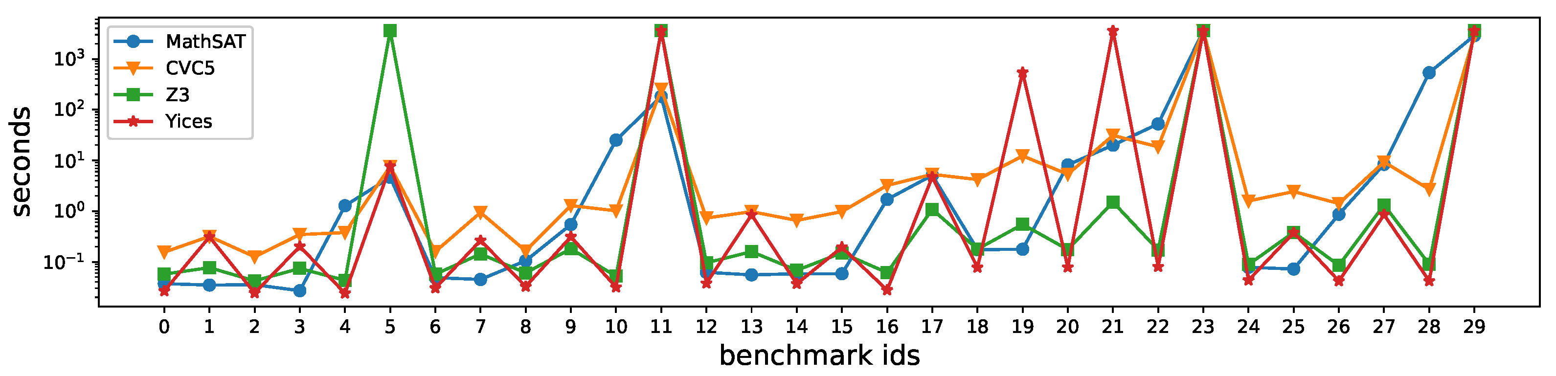
Regarding the performances of the different solvers, MathSAT managed to successfully solve the greatest number of benchmarks, followed by CVC5, Z3, and Yices2. From Figure 2, it is possible to notice that, while MathSAT and CVC5 managed to solve the greatest number of queries, both Z3 and Yices2 often need less time than the other solver to reach the results on the queries they are able to solve before the timeout. Overall, it seems that CVC5 and MathSAT are the best suited for the task of verification of neural networks. While this result is not particularly surprising for the case of CVC5, as the winner of the QF_NRA division in the Single Query Track of SMT-COMP 2022, MathSAT behaved better than expected given its modest positioning in the same competition.

5. Related Works

In the last few years, many different methodologies and tools tackling the verification of neural networks have been developed, as testified to in [9,22,42,43]. For the sake of clarity, first we briefly explain the difference between complete and incomplete verification methodologies; then, we provide a more detailed overview of the existing methodologies following the categorization proposed in [42], in which they are classified based on the kind of guarantee they can provide.

Incomplete verification methodologies [14,15,16,44,45] are typically based on technologies such as abstract interpretation and bound propagation. As a consequence, their answers regarding the validity of a property of interest are usually subject to a certain degree of uncertainty. This problem originates from the use of over-approximations of the original network $\nu$ in the verification methodology, which, as consequence, may be unable to distinguish between the presence of a spurious counter-example, caused by the coarseness of the approximation, and a concrete one. However, it should be noted that the use of over-approximations, while potentially causing the above-mentioned issue, allows for the successful verification of networks of significant complexity. Conversely, complete verification methodologies [10,17,19,46,47] traditionally leverage techniques such as mixed integer linear programming (MILP), branch and bound, and satisfiability modulo theories to provide a conclusive answer regarding the validity of the property of interest, at the price of greatly increased computational complexity.

As mentioned before, another important categorization for verification methodology is the one based on the kind of guarantees they are able to provide: here, we focus on deterministic, one-sided, and converging guarantees. Methodologies providing deterministic guarantees, which state exactly whether a property is valid, typically transform the verification problem into a set of constraints that are then solved by a suitable solver. As an example, the methodologies presented in [10,34,48] leverage SMT solvers, whereas in [17,19,46] mixed integer linear programming (MILP) solvers are used. However, the most recent methodologies often enhance such solvers with other techniques such as branch-and-bound (BnB) and symbolic bound propagation. One-sided guarantees can serve as a sufficient condition for a property to hold by providing either a lower or an upper bound to a variable. Typically, the approaches offering this kind of guarantee present better scalability than the previously presented ones and are more resilient to issues of numerical instability that may arise due to the intrinsic limitation of the accuracy of floating-point arithmetic. Such methodologies leverage technologies such as linear approximation [45,49], convex optimization [50], abstract interpretation [14,15,16], and interval analysis [8]. Lastly, the approaches providing guarantees with converging lower and upper bounds also achieve good scalability by leveraging technologies such as global optimization [51,52], layer-by-layer refinement and analysis [53] and reduction to a two-player turn-based game [54,55]. In

Table 3. Summary of different contributions for verification of neural networks in the scientific literature. The column Guarantees represents the kind of guarantees provided by the verification methodologies. Technology represents the main technology leveraged by the methodologies, whereas Methodology represents the corresponding papers. Finally, Completeness indicates if the related methodology is complete (✓) or incomplete (×).

Guarantees	Technology	Methodology	Completeness
Deterministic	SMT	Katz et al. [10]	✓
		Pulina and Tacchella [48]	×
		Ehlers [34]	✓
	MILP	Henriksen and Lomuscio [17]	✓
		Henriksen and Lomuscio [19]	✓
		Bunel et al. [46]	✓
One sided	Abstract Interpretation	Guidotti et al. [16]	×
		Singh et al. [14]	×
		Tran et al. [15]	×
	Convex Optimization	Wong and Kolter [50]	×
	Interval Analysis	Wang et al. [8]	×
	Linear Approximation	Zhang et al. [45]	×
		Weng et al. [49]	×
Converging	Layer-by-Layer Refinement	Huang et al. [53]	✓
	Two-Player Game	Wu et al. [54]	×
		Wicker et al. [55]	×
	Global Optimization	Ruan et al. [51]	×
		Ruan et al. [52]	×

, we provide a summary of the current approaches; for a more extensive survey, we refer to [42].

While both the categorizations presented are still widely used, many new verification tools combine complete and incomplete algorithms to achieve a better trade-off between computational complexity and accuracy. Furthermore, they often provide various kinds of guarantees. As a consequence, our categorization may present some small inaccuracies: for example, the two methodologies of [15,16], which are classified as incomplete, may be complete under certain conditions and modes of operation. Moreover, while their main technology is abstract interpretation, some of their internal algorithms make use also of linear programming.

Concerning the usage of SMT technologies in the verification of neural networks, the first paper [48] presenting a verification methodology leveraging SMT dates back to 2010: in particular, the tool NeVer used in combination with the HySAT [56] solver and abstract interpretation to verify a small fully connected neural network with a single layer (with three hidden neurons) of sigmoid activation functions. Then, in 2012, the same authors proposed an enhancement of their algorithm and compared its performances with a portfolio of SMT solvers using a set of benchmarks considering various properties and network architectures of interest. After the discovery of adversarial perturbation in 2013 by [28], a novel methodology leveraging both linear programming and SMT technologies was proposed [34] in 2017. This verification algorithm used a particular encoding of the network and property of interest to enhance the performances of the solvers, making it possible to verify multi-layer fully connected NNs with ReLU activation functions. Lastly, still in 2017, a methodology leveraging a novel $\mathcal{T}$-solver, optimized for managing ReLU activation functions, was proposed in [35]. The algorithm was tested successfully on the ACAS XU benchmark, which consists of a set of networks and related properties from the aviation domain.

6. Conclusions

In this paper, we conducted an experimental evaluation of several state-of-the-art SMT solvers. Our evaluation utilized a set of benchmarks consisting of various neural network architectures, non-linear activation functions, and different properties of interest. The neural networks were trained on real sensor data obtained from an electric motor, resulting in realistic accuracy levels. The properties of interest focused on local robustness and included varying maximum magnitudes for perturbations and tolerable output deviations.

Our findings indicate that, currently, even the solvers that support transcendent functions struggle to reliably verify networks with such activation functions. Specifically, among the solvers we evaluated, only MathSAT was able to complete the analysis for a few benchmarks with logistic activation functions before reaching the timeout limit. However, when we considered piece-wise linear ReLU activation functions, the solvers performed better. In the worst-case scenario, at least 26 out of 30 benchmarks were solved correctly, with the best solver successfully solving 29 benchmarks. Based on our evaluation, we conclude that MathSAT and CVC5 are the most suitable solvers for the verification of neural networks.

In our future endeavors, as future work, we intend to extend our experimental evaluation by including additional case studies derived from the IMOCO4.E project. This extension will enable us to investigate a broader spectrum of network architectures and their suitability for various domains. Moreover, we are actively engaged in ongoing research to enhance existing verification methodologies that rely on abstract interpretation.

References

- Giunchiglia, E.; Nemchenko, A.; van der Schaar, M. RNN-SURV: A Deep Recurrent Model for Survival Analysis. In Proceedings of the Artificial Neural Networks and Machine Learning—ICANN 2018—27th International Conference on Artificial Neural Networks, Rhodes, Greece, 4–7 October 2018; Springer: Berlin/Heidelberg, Germany, 2018; Volume 11141, pp. 23–32. [Google Scholar]
- Liu, W.; Wang, Z.; Liu, X.; Zeng, N.; Liu, Y.; Alsaadi, F.E. A survey of deep neural network architectures and their applications. Neurocomputing 2017, 234, 11–26. [Google Scholar] [CrossRef]
- Arrieta, A.B.; Rodríguez, N.D.; Ser, J.D.; Bennetot, A.; Tabik, S.; Barbado, A.; García, S.; Gil-Lopez, S.; Molina, D.; Benjamins, R.; et al. Explainable Artificial Intelligence (XAI): Concepts, taxonomies, opportunities and challenges toward responsible AI. Inf. Fusion 2020, 58, 82–115. [Google Scholar] [CrossRef] [Green Version]
- Zhang, Q.; Zhu, S. Visual interpretability for deep learning: A survey. Frontiers Inf. Technol. Electron. Eng. 2018, 19, 27–39. [Google Scholar] [CrossRef] [Green Version]
- Samek, W.; Montavon, G.; Lapuschkin, S.; Anders, C.J.; Müller, K. Explaining Deep Neural Networks and Beyond: A Review of Methods and Applications. Proc. IEEE 2021, 109, 247–278. [Google Scholar] [CrossRef]
- Ferrari, C.; Müller, M.N.; Jovanovic, N.; Vechev, M.T. Complete Verification via Multi-Neuron Relaxation Guided Branch-and-Bound. In Proceedings of the Tenth International Conference on Learning Representations, ICLR 2022, Virtual Event, 25–29 April 2022. [Google Scholar]
- Demarchi, S.; Guidotti, D.; Pitto, A.; Tacchella, A. Formal Verification Of Neural Networks: A Case Study About Adaptive Cruise Control. In Proceedings of the 36th ECMS International Conference on Modelling and Simulation, ECMS 2022, Ålesund, Norway, 30 May–3 June 2022; pp. 310–316. [Google Scholar]
- Wang, S.; Zhang, H.; Xu, K.; Lin, X.; Jana, S.; Hsieh, C.; Kolter, J.Z. Beta-CROWN: Efficient Bound Propagation with Per-neuron Split Constraints for Neural Network Robustness Verification. In Proceedings of the Advances in Neural Information Processing Systems 34: Annual Conference on Neural Information Processing Systems 2021, NeurIPS 2021, Virtual, 6–14 December 2021; Curran Associates, Inc.: Red Hook, NY, USA, 2021; pp. 29909–29921. [Google Scholar]
- Guidotti, D. Safety Analysis of Deep Neural Networks. In Proceedings of the Thirtieth International Joint Conference on Artificial Intelligence, IJCAI 2021, Montreal, QC, Canada, 19–27 August 2021; pp. 4887–4888. [Google Scholar]
- Katz, G.; Huang, D.A.; Ibeling, D.; Julian, K.; Lazarus, C.; Lim, R.; Shah, P.; Thakoor, S.; Wu, H.; Zeljic, A.; et al. The Marabou Framework for Verification and Analysis of Deep Neural Networks. In Proceedings of the Computer Aided Verification—31st International Conference, CAV 2019, New York, NY, USA, 15–18 July 2019; Volume 11561, pp. 443–452. [Google Scholar]
- Guidotti, D. Enhancing Neural Networks through Formal Verification. In Proceedings of the Discussion and Doctoral Consortium papers of AI*IA 2019—18th International Conference of the Italian Association for Artificial Intelligence, Rende, Italy, 19–22 November 2019; Volume 2495, pp. 107–112. [Google Scholar]
- Bak, S.; Tran, H.; Hobbs, K.; Johnson, T.T. Improved Geometric Path Enumeration for Verifying ReLU Neural Networks. In Proceedings of the Computer Aided Verification—32nd International Conference, CAV 2020, Los Angeles, CA, USA, 21–24 July 2020; Springer: Berlin/Heidelberg, Germany, 2020; Volume 12224, pp. 66–96. [Google Scholar]
- Kouvaros, P.; Kyono, T.; Leofante, F.; Lomuscio, A.; Margineantu, D.D.; Osipychev, D.; Zheng, Y. Formal Analysis of Neural Network-Based Systems in the Aircraft Domain. In Proceedings of the Formal Methods—24th International Symposium, FM 2021, Virtual Event, 20–26 November 2021; Springer: Berlin/Heidelberg, Germany, 2021; Volume 13047, pp. 730–740. [Google Scholar]
- Singh, G.; Gehr, T.; Püschel, M.; Vechev, M.T. An abstract domain for certifying neural networks. Proc. ACM Program. Lang. 2019, 3, 41:1–41:30. [Google Scholar] [CrossRef] [Green Version]
- Tran, H.; Yang, X.; Lopez, D.M.; Musau, P.; Nguyen, L.V.; Xiang, W.; Bak, S.; Johnson, T.T. NNV: The Neural Network Verification Tool for Deep Neural Networks and Learning-Enabled Cyber-Physical Systems. In Proceedings of the Computer Aided Verification—32nd International Conference, CAV 2020, Los Angeles, CA, USA, 21–24 July 2020; Springer: Berlin/Heidelberg, Germany, 2020; Volume 12224, pp. 3–17. [Google Scholar]
- Guidotti, D.; Pulina, L.; Tacchella, A. pyNeVer: A Framework for Learning and Verification of Neural Networks. In Proceedings of the Automated Technology for Verification and Analysis—19th International Symposium, ATVA 2021, Gold Coast, QLD, Australia, 18–22 October 2021; Springer: Berlin/Heidelberg, Germany, 2021; Volume 12971, pp. 357–363. [Google Scholar]
- Henriksen, P.; Lomuscio, A.R. Efficient Neural Network Verification via Adaptive Refinement and Adversarial Search. In Proceedings of the ECAI 2020—24th European Conference on Artificial Intelligence, Including 10th Conference on Prestigious Applications of Artificial Intelligence (PAIS 2020), Santiago de Compostela, Spain, 29 August–8 September 2020; IOS Press: Amsterdam, The Netherlands, 2020; Volume 325, pp. 2513–2520. [Google Scholar]
- Guidotti, D.; Leofante, F.; Pulina, L.; Tacchella, A. Verification and Repair of Neural Networks: A Progress Report on Convolutional Models. In Proceedings of the AI*IA 2019—Advances in Artificial Intelligence—XVIIIth International Conference of the Italian Association for Artificial Intelligence, Rende, Italy, 19–22 November 2019; Springer: Berlin/Heidelberg, Germany, 2019; Volume 11946, pp. 405–417. [Google Scholar]
- Henriksen, P.; Lomuscio, A. DEEPSPLIT: An Efficient Splitting Method for Neural Network Verification via Indirect Effect Analysis. In Proceedings of the Thirtieth International Joint Conference on Artificial Intelligence, IJCAI 2021, Montreal, QC, Canada, 19–27 August 2021; pp. 2549–2555. [Google Scholar]
- Guidotti, D.; Leofante, F.; Pulina, L.; Tacchella, A. Verification of Neural Networks: Enhancing Scalability Through Pruning. In Proceedings of the ECAI 2020—24th European Conference on Artificial Intelligence, Including 10th Conference on Prestigious Applications of Artificial Intelligence (PAIS 2020), Santiago de Compostela, Spain, 29 August– 8 September 2020; IOS Press: Amsterdam, The Netherlands, 2020; Volume 325, pp. 2505–2512. [Google Scholar]
- Henriksen, P.; Leofante, F.; Lomuscio, A. Repairing misclassifications in neural networks using limited data. In Proceedings of the SAC ’22: The 37th ACM/SIGAPP Symposium on Applied Computing, Virtual Event, 25–29 April 2022; ACM: New York, NY, USA, 2022; pp. 1031–1038. [Google Scholar]
- Guidotti, D. Verification and Repair of Neural Networks. In Proceedings of the Thirty-Fifth AAAI Conference on Artificial Intelligence, AAAI 2021, Thirty-Third Conference on Innovative Applications of Artificial Intelligence, IAAI 2021, The Eleventh Symposium on Educational Advances in Artificial Intelligence, EAAI 2021, Virtual Event, 2–9 February 2021; AAAI Press: Washington, DC, USA, 2021; pp. 15714–15715. [Google Scholar]
- Sotoudeh, M.; Thakur, A.V. Provable repair of deep neural networks. In Proceedings of the PLDI ’21: 42nd ACM SIGPLAN International Conference on Programming Language Design and Implementation, Virtual Event, 20–25 June 2021; ACM: New York, NY, USA, 2021; pp. 588–603. [Google Scholar]
- Goldberger, B.; Katz, G.; Adi, Y.; Keshet, J. Minimal Modifications of Deep Neural Networks using Verification. In Proceedings of the LPAR 2020: 23rd International Conference on Logic for Programming, Artificial Intelligence and Reasoning, Alicante, Spain, 22–27 May 2020; Volume 73, pp. 260–278. [Google Scholar]
- Guidotti, D.; Leofante, F.; Tacchella, A.; Castellini, C. Improving Reliability of Myocontrol Using Formal Verification. IEEE Trans. Neural Syst. Rehabil. Eng. 2019, 27, 564–571. [Google Scholar] [CrossRef] [PubMed]
- Guidotti, D.; Leofante, F. Repair of Convolutional Neural Networks using Convex Optimization: Preliminary Experiments. In Proceedings of the Cyber-Physical Systems PhD Workshop 2019, an Event Held within the CPS Summer School “Designing Cyber-Physical Systems—From Concepts to Implementation”, Alghero, Italy, 23 September 2019; Volume 2457, pp. 18–28. [Google Scholar]
- Guidotti, D.; Leofante, F.; Castellini, C.; Tacchella, A. Repairing Learned Controllers with Convex Optimization: A Case Study. In Proceedings of the Integration of Constraint Programming, Artificial Intelligence, and Operations Research—16th International Conference, CPAIOR 2019, Thessaloniki, Greece, 4–7 June 2019; Springer: Berlin/Heidelberg, Germany, 2019; Volume 11494, pp. 364–373. [Google Scholar]
- Szegedy, C.; Zaremba, W.; Sutskever, I.; Bruna, J.; Erhan, D.; Goodfellow, I.J.; Fergus, R. Intriguing properties of neural networks. In Proceedings of the 2nd International Conference on Learning Representations, ICLR 2014, Banff, AB, Canada, 14–16 April 2014. [Google Scholar]
- Psarommatis, F.; May, G.; Azamfirei, V. Envisioning maintenance 5.0: Insights from a systematic literature review of Industry 4.0 and a proposed framework. J. Manuf. Syst. 2023, 68, 376–399. [Google Scholar] [CrossRef]
- Cech, M.; Beltman, A.; Ozols, K. Digital Twins and AI in Smart Motion Control Applications. In Proceedings of the 27th IEEE International Conference on Emerging Technologies and Factory Automation, ETFA 2022, Stuttgart, Germany, 6–9 September 2022; pp. 1–7. [Google Scholar]
- Barrett, C.; Stump, A.; Tinelli, C. The SMT-LIB standard: Version 2.0. In Proceedings of the SMT Workshop 2010, Edinburgh, UK, 14–15 July 2010; Volume 13, p. 14. [Google Scholar]
- de Moura, L.M.; Bjørner, N.S. Satisfiability modulo theories: Introduction and applications. Commun. ACM 2011, 54, 69–77. [Google Scholar] [CrossRef]
- Pulina, L.; Tacchella, A. Challenging SMT solvers to verify neural networks. AI Commun. 2012, 25, 117–135. [Google Scholar] [CrossRef]
- Ehlers, R. Formal Verification of Piece-Wise Linear Feed-Forward Neural Networks. In Proceedings of the Automated Technology for Verification and Analysis—15th International Symposium, ATVA 2017, Pune, India, 3–6 October 2017; Springer: Berlin/Heidelberg, Germany, 2017; Volume 10482, pp. 269–286. [Google Scholar]
- Katz, G.; Barrett, C.W.; Dill, D.L.; Julian, K.; Kochenderfer, M.J. Reluplex: An Efficient SMT Solver for Verifying Deep Neural Networks. In Proceedings of the Computer Aided Verification—29th International Conference, CAV 2017, Heidelberg, Germany, 24–28 July 2017; Springer: Berlin/Heidelberg, Germany, 2017; Volume 10426, pp. 97–117. [Google Scholar]
- Kirchgässner, W.; Wallscheid, O.; Böcker, J. Estimating Electric Motor Temperatures With Deep Residual Machine Learning. IEEE Trans. Power Electron. 2021, 36, 7480–7488. [Google Scholar] [CrossRef]
- Wallscheid, O.; Böcker, J. Global Identification of a Low-Order Lumped-Parameter Thermal Network for Permanent Magnet Synchronous Motors. IEEE Trans. Energy Convers. 2016, 31, 354–365. [Google Scholar] [CrossRef]
- Barbosa, H.; Barrett, C.W.; Brain, M.; Kremer, G.; Lachnitt, H.; Mann, M.; Mohamed, A.; Mohamed, M.; Niemetz, A.; Nötzli, A.; et al. cvc5: A Versatile and Industrial-Strength SMT Solver. In Proceedings of the Tools and Algorithms for the Construction and Analysis of Systems—28th International Conference, TACAS 2022, Held as Part of the European Joint Conferences on Theory and Practice of Software, ETAPS 2022, Munich, Germany, 2–7 April 2022; Springer: Berlin/Heidelberg, Germany, 2022; Volume 13243, pp. 415–442. [Google Scholar]
- Cimatti, A.; Griggio, A.; Schaafsma, B.J.; Sebastiani, R. The MathSAT5 SMT Solver. In Proceedings of the Tools and Algorithms for the Construction and Analysis of Systems—19th International Conference, TACAS 2013, Held as Part of the European Joint Conferences on Theory and Practice of Software, ETAPS 2013, Rome, Italy, 16–24 March 2013; Springer: Berlin/Heidelberg, Germany, 2013; Volume 7795, pp. 93–107. [Google Scholar]
- de Moura, L.M.; Bjørner, N.S. Z3: An Efficient SMT Solver. In Proceedings of the Tools and Algorithms for the Construction and Analysis of Systems, 14th International Conference, TACAS 2008, Held as Part of the Joint European Conferences on Theory and Practice of Software, ETAPS 2008, Budapest, Hungary, 29 March–6 April 2008; Springer: Berlin/Heidelberg, Germany, 2008; Volume 4963, pp. 337–340. [Google Scholar]
- Dutertre, B. Yices 2.2. In Proceedings of the Computer Aided Verification—26th International Conference, CAV 2014, Held as Part of the Vienna Summer of Logic, VSL 2014, Vienna, Austria, 18–22 July 2014; Springer: Berlin/Heidelberg, Germany, 2014; Volume 8559, pp. 737–744. [Google Scholar]
- Huang, X.; Kroening, D.; Ruan, W.; Sharp, J.; Sun, Y.; Thamo, E.; Wu, M.; Yi, X. A survey of safety and trustworthiness of deep neural networks: Verification, testing, adversarial attack and defence, and interpretability. Comput. Sci. Rev. 2020, 37, 100270. [Google Scholar] [CrossRef]
- Leofante, F.; Narodytska, N.; Pulina, L.; Tacchella, A. Automated Verification of Neural Networks: Advances, Challenges and Perspectives. arXiv 2018, arXiv:1805.09938. [Google Scholar]
- Pulina, L.; Tacchella, A. NeVer: A tool for artificial neural networks verification. Ann. Math. Artif. Intell. 2011, 62, 403–425. [Google Scholar] [CrossRef]
- Zhang, H.; Weng, T.; Chen, P.; Hsieh, C.; Daniel, L. Efficient Neural Network Robustness Certification with General Activation Functions. In Proceedings of the Advances in Neural Information Processing Systems 31: Annual Conference on Neural Information Processing Systems 2018, NeurIPS 2018, Montréal, QC, Canada, 3–8 December 2018; pp. 4944–4953. [Google Scholar]
- Bunel, R.; Lu, J.; Turkaslan, I.; Torr, P.H.S.; Kohli, P.; Kumar, M.P. Branch and Bound for Piecewise Linear Neural Network Verification. J. Mach. Learn. Res. 2020, 21, 42:1–42:39. [Google Scholar]
- Palma, A.D.; Bunel, R.; Desmaison, A.; Dvijotham, K.; Kohli, P.; Torr, P.H.S.; Kumar, M.P. Improved Branch and Bound for Neural Network Verification via Lagrangian Decomposition. arXiv 2021, arXiv:2104.06718. [Google Scholar]
- Pulina, L.; Tacchella, A. An Abstraction-Refinement Approach to Verification of Artificial Neural Networks. In Proceedings of the Computer Aided Verification, 22nd International Conference, CAV 2010, Edinburgh, UK, 15–19 July 2010; Springer: Berlin/Heidelberg, Germany, 2010; Volume 6174, pp. 243–257. [Google Scholar]
- Weng, T.; Zhang, H.; Chen, H.; Song, Z.; Hsieh, C.; Daniel, L.; Boning, D.S.; Dhillon, I.S. Towards Fast Computation of Certified Robustness for ReLU Networks. In Proceedings of the 35th International Conference on Machine Learning, ICML 2018, Stockholmsmässan, Stockholm, Sweden, 10–15 July 2018; Volume 80, pp. 5273–5282. [Google Scholar]
- Wong, E.; Kolter, J.Z. Provable Defenses against Adversarial Examples via the Convex Outer Adversarial Polytope. In Proceedings of the 35th International Conference on Machine Learning, ICML 2018, Stockholmsmässan, Stockholm, Sweden, 10–15 July 2018; Volume 80, pp. 5283–5292. [Google Scholar]
- Ruan, W.; Huang, X.; Kwiatkowska, M. Reachability Analysis of Deep Neural Networks with Provable Guarantees. In Proceedings of the Twenty-Seventh International Joint Conference on Artificial Intelligence, IJCAI 2018, Stockholm, Sweden, 13–19 July 2018; pp. 2651–2659. [Google Scholar]
- Ruan, W.; Wu, M.; Sun, Y.; Huang, X.; Kroening, D.; Kwiatkowska, M. Global Robustness Evaluation of Deep Neural Networks with Provable Guarantees for the Hamming Distance. In Proceedings of the Twenty-Eighth International Joint Conference on Artificial Intelligence, IJCAI 2019, Macao, China, 10–16 August 2019; pp. 5944–5952. [Google Scholar]
- Huang, X.; Kwiatkowska, M.; Wang, S.; Wu, M. Safety Verification of Deep Neural Networks. In Proceedings of the Computer Aided Verification—29th International Conference, CAV 2017, Heidelberg, Germany, 24–28 July 2017; Springer: Berlin/Heidelberg, Germany, 2017; Volume 10426, pp. 3–29. [Google Scholar]
- Wu, M.; Wicker, M.; Ruan, W.; Huang, X.; Kwiatkowska, M. A game-based approximate verification of deep neural networks with provable guarantees. Theor. Comput. Sci. 2020, 807, 298–329. [Google Scholar] [CrossRef]
- Wicker, M.; Huang, X.; Kwiatkowska, M. Feature-Guided Black-Box Safety Testing of Deep Neural Networks. In Proceedings of the Tools and Algorithms for the Construction and Analysis of Systems—24th International Conference, TACAS 2018, Held as Part of the European Joint Conferences on Theory and Practice of Software, ETAPS 2018, Thessaloniki, Greece, 14–20 April 2018; Springer: Berlin/Heidelberg, Germany, 2018; Volume 10805, pp. 408–426. [Google Scholar]
- Fränzle, M.; Herde, C. HySAT: An efficient proof engine for bounded model checking of hybrid systems. Form. Methods Syst. Des. 2007, 30, 179–198. [Google Scholar] [CrossRef]
Figure 2.
Logarithmic representation of the times needed to solve the benchmarks (shown on the x-axis) by the solvers.