

Segmentation Method of Magnetoelectric Brain Image Based on the Transformer and the CNN

School of Control and Computer Engineering, North China Electric Power University, Baoding 071003, China
*
Author to whom correspondence should be addressed.
Information 2022, 13(10), 445; https://doi.org/10.3390/info13100445
Submission received: 8 August 2022
/
Revised: 15 September 2022
/
Accepted: 20 September 2022
/
Published: 23 September 2022
(This article belongs to the Special Issue Advances in Medical Image Analysis and Deep Learning)
Abstract
:To address the problem of a low accuracy and blurred boundaries in segmenting multimodal brain tumor images using the TransBTS network, a 3D BCS_T model incorporating a channel space attention mechanism is proposed. Firstly, the TransBTS model hierarchy is increased to obtain more local feature information, and residual basis blocks are added to reduce feature loss. Secondly, downsampling is incorporated into the hybrid attention mechanism to enhance the critical region information extraction. Finally, weighted cross-entropy loss and generalized dice loss are employed to solve the inequality problem in the tumor sample categories. The experimental results show that the whole tumor region WT, the tumor core region TC, and the enhanced tumor region ET are improved by an average of 2.53% in the evaluation metric of the Dice similarity coefficient, compared with the TransBTS network and shortened by an average of 3.14 in the metric of Hausdorff distance 95. Therefore, the 3D BCS_T model can effectively improve the segmentation accuracy and boundary clarity of both the tumor core and the enhanced tumor categories of the small areas.
1. Introduction
Brain tumors are irregular and uncontrollable clusters of cells that grow in the brain. A tumor is usually latent in the brain of patients in various forms, with a high incidence [1]. The accurate segmentation of tumor categories can directly affect the clinical diagnosis results and subsequent treatment plans. Magnetic Resonance Imaging (MRI) is a biomagnetic nuclear spin imaging technology that forms with the development of electronic circuit technology and superconductor technology. It can enable medical experts to detect images in a shorter amount of time [2]. Among them, brain tumor MRI contains the four modalities of T1-weighted imaging (T1), T2-weighted imaging (T2), fluid attenuated inversion recovery (FLAIR), and T1-weighted imaging with a contrast medium (T1ce). The physician manually delineates three parts of the tumor in combination with the degree of highlighting in the MRI and his own experience, namely: (1) the enhanced tumor (ET); (2) the tumor core (TC) is typically the area to be resected, which consists of the ET and the necrotic tumor (NET); (3) the whole tumor (WT) describes the integrity of the disease which comprises the ET, NET, and the edematous area (ED). However, the increasing number of patients is leading to a surge in magneto-optical images, and the manual segmentation relies on personal experience with a low reproducibility. Therefore, designing an automatic segmentation algorithm model with a high accuracy and strong robustness will be of great significance in diagnosing and treating brain tumors.
Currently, the mainstream MRI architecture for brain tumor segmentation includes a convolutional neural network model framework represented by encoder-decoder architecture [3,4,5,6,7] and the integration framework of the transformer model and convolutional neural network represented by the attention mechanism [8,9,10]. Kamnitsas et al. [4] proposed a 3D DeepMedic network to address the poor segmentation of 2D series networks. The literature [5] presented a modified robust fuzzy c-means (MRFCM) algorithm that requires slicing brain tumor images and from which, it is challenging to learn global information. The study [6] put forward a convolutional neural network (CNN) segmentation method based on small image blocks, which enable the model to focus more on the local structural features of the image but fail to fuse the multimodal information well and ignores the information features among the modalities. Henry et al. [7] proposed a 3D Unet model for brain tumor segmentation that can input full-volume images. Still, the pooling and downsampling in the coding process can cause the image loss of fine-grained information. In 2020, the self-attention mechanism in the Transformer model introduced by Dosovitskiy et al. [8] could compensate for the shortcomings of CNNs by focusing on the global information. TransUnet [9] is the first model that integrates the transformer self-attention mechanism and convolutional neural network CNN. Although used for brain tumor segmentation, it is semi-supervised learning because it relies on pre-trained models and requires pre-trained weights from large natural image datasets. TransBTS [10] was an integrated 3D brain tumor segmentation model trained from end to end. However, this model only uses the Softmax loss function. The increase of one label prediction will suppress the prediction probability of other labels, which is difficult for small target segmentation.
Considering the existing network segmentation of multi-modal brain tumor images is not accurate, the boundary is blurred, and the use of the TransBTS single loss function is not ideal for small target segmentation. Therefore, we propose a segmentation network based on the TransBTS model, which is based on a CNN and incorporates the latest transformer auto-attention coding section. A five-channel end-to-end, fully automated unsupervised learning network is constructed by improving the residual basis block, the channel space mixed domain attention mechanism, and the hybrid loss function. This model can effectively improve the segmentation performance of the model, especially the accuracy of small target tumor segmentation. The main contributions of this study are as follows.
- The residual basis block replaces the traditional stepwise convolution operation, effectively performing deep feature extraction on the original features and maximizing the retention of more learnable feature information.
- The 3D BCS channel of the spatially mixed domain attention mechanism module suppresses the tumor irrelevant region information in MRI images, enables more targeted feature extraction, and improves the segmentation limit.
- The encoder operation of Vision Transformer enhances the feature fusion capability to obtain more meaningful information, thus further improving the segmentation accuracy of the algorithm.
- The coupling of two loss functions can enhance the segmentation accuracy of small targets and improve the problem of extreme imbalances in lesion classes.
- The recently released BraTS2021 dataset is used as a benchmark. The advantages of the 3D BCS_T algorithm model are demonstrated through a series of comparison experiments and ablation experiments, which provide more robust diagnostic results.
The rest of the paper is organized as follows. Section 2 explains the original TransBTS model and the structure of our proposed 3D BCS_T model. Section 3 describes the three improved modules, illustrating the dataset and the image processing steps. In Section 4, we have improved the comparative model and conducted several experiments. The proposed model is analyzed qualitatively and quantitatively to verify its validity. Finally, Section 5 concludes the paper and provides the following steps to be taken.
2. Network Model Construction
2.1. TransBTS Network Architecture
The TransBTS network is a four-layer U-shaped structure based on an encoder-decoder. Firstly, the CNN is used to extract spatial features. Then, through the down-sampling operation with a convolution kernel size of 3, a convolution step size of 2, and a feature image filling the width of 1, the image size is reduced to a second of the previous size. The feature image dimension is expanded to twice the original size. The bottom uses the self-attention mechanism in the transformer model for the global feature modeling.
Similarly, after jumping and connecting with the encoder of the corresponding layer, the sampling layer and the deconvolution layer are gradually stacked to produce high-resolution segmentation results. However, these operations in the TransBTS network will, according to some feature information, and coupled with the particularity of multimodal images, result in the unclear boundary of the segmentation results. Therefore, a 3D BCS_T model is proposed by improving the encoder and decoder, respectively.
2.2. 3D BCS_T Network Architecture
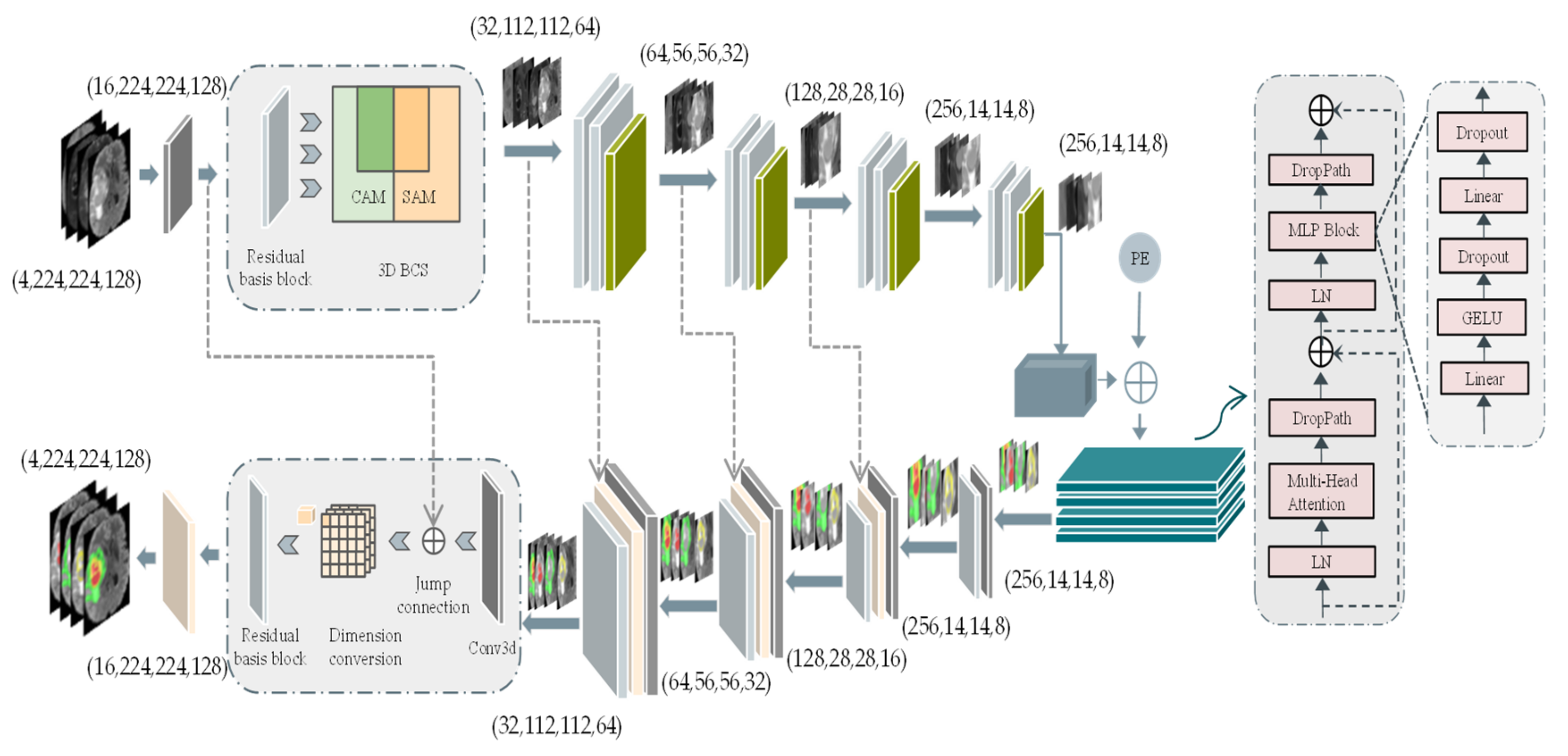
The 3D BCS_T model is subdivided into three parts: the encoder process, the transformer fusion process, and the decoder process. The overall architecture is shown in Figure 1.
As can be seen in Figure 1, the CAM focuses its attention on the meaningful feature channels, and the SAM focuses on the noteworthy spatial features, which collaborate well to form the 3D BCS block. The weights of pixels in the different channels and the pixels in various positions of the same channel are considered comprehensively to obtain a more discriminative feature representation. In addition, the PE is nested after the feature image to form a new one-dimensional feature image as the input to the transformer’s autoencoder. The PE is nested after the feature image to form a new one-dimensional feature image as the input to the transformer’s autoencoder.
The first thing is the encoder process: the input four-modality MRI voxel block (4, 224, 224, 128) cropped by the origin center, where 4 indicates the number of modalities and (224, 224, 128) represents the length, width, and depth of the voxel block, respectively. A feature image with a channel count of 16 is formed after a convolution kernel size of 3 × 3 × 3. Each encoder layer contains a residual basis module and a 3D BCS hybrid domain attention mechanism module. Following each layer, the image size is reduced to one-half of the original size, and the feature image dimension is expanded to twice the original size.
The bottom feature L (256, 14, 14, 8) obtains global information through the transformer algorithm. The 3 × 3 × 3 convolution kernel is used to increase the feature dimension from 256 to 512, and the image size is decomposed into a feature graph G of a one-dimensional sequence (14 × 14 × 8). Then, the linear embedding sequences (512, 14 × 14 × 8) of these image blocks are superimposed with the learned position coding (1, 14 × 14 × 8) as the input of the transformer encoder. The four transformer layers of the transformer encoder consist of the multi-headed attention at the interaction level (MHA) blocks and the feedforward networks.
The upsampling deconvolution operation is performed similarly to the downsampling, with each upsampling decreasing the feature dimension and increasing the image size. The final feature image with a high resolution (16, 224, 224, 128) is obtained by stacking the channels and several deconvolution times. The image size with four labeled channels is accepted as the model’s output through a 1 × 1 × 1 convolution operation and Softmax activation function.
3. Related Work
Table 1 lists the representative articles by researchers in recent years for tumor segmentation, comparing them in terms of data volume size (D.V.S.), data enhancement (D.E.), residual connectivity (R.C.), attention mechanism optimization (A.M.O), and loss function optimization (L.F.O).
We can see that the traditional CNN-based individual network models can no longer meet high-performance requirements. The pooling and downsampling of the network model in paper [7] in the coding process will cause the loss of fine-grained information about the image. The VoxResNet applies the ResNet network idea to the 3D brain MRI segmentation [11], and experiments confirm that the residual module can effectively perform the deep feature extraction on the original features, which helps to identify the feature information better. It can alleviate the information loss caused by the increase of network layers. However, with only 20 patients, the amount of data is too small. Research has the disadvantages of small data sizes and poor network robustness in terms of data volume usage. It is found that only half of the studies [7,10,13,15] used data augmentation techniques to augment the data sample set. The TransBTS integrates the multi-scale information through the vision transformer algorithm, but using a single loss function is not ideal for small target segmentation [10]. The mixed loss function of Dice loss and Jaccard loss is proposed in the literature [13]. However, the Dice loss is suitable for the binary classification but not for the multi-class tumor segmentation. Therefore, the fact that the proposed network adequately considers these four aspects, is noteworthy. The BraTS2021 dataset, on the one hand, has a training set three times larger than the BraTS2020 training set, which facilitates the training of the model fit. A residual base block is designed in the encoder part of the network model to reduce the loss of essential parameters in the propagation process. Furthermore, it is proposed that the 3D BCS mixed attention module can enhance the space feature extraction ability by optimizing the attention mechanism. The bottom layer integrates the multi-scale information through the vision transformer algorithm. Finally, a combination of the multi-category GDL and the weighted cross-entropy loss function is proposed to solve the problem of imbalanced imaging categories. The advantages of the 3D BCS_T algorithm model are demonstrated through a series of comparative experiments and the ablation experiments studied and analyzed to provide more robust diagnostic results.
3.1. Fundamentals of the Improved Algorithm
3.1.1. 3D BCS Hybrid Domain Attention Mechanism
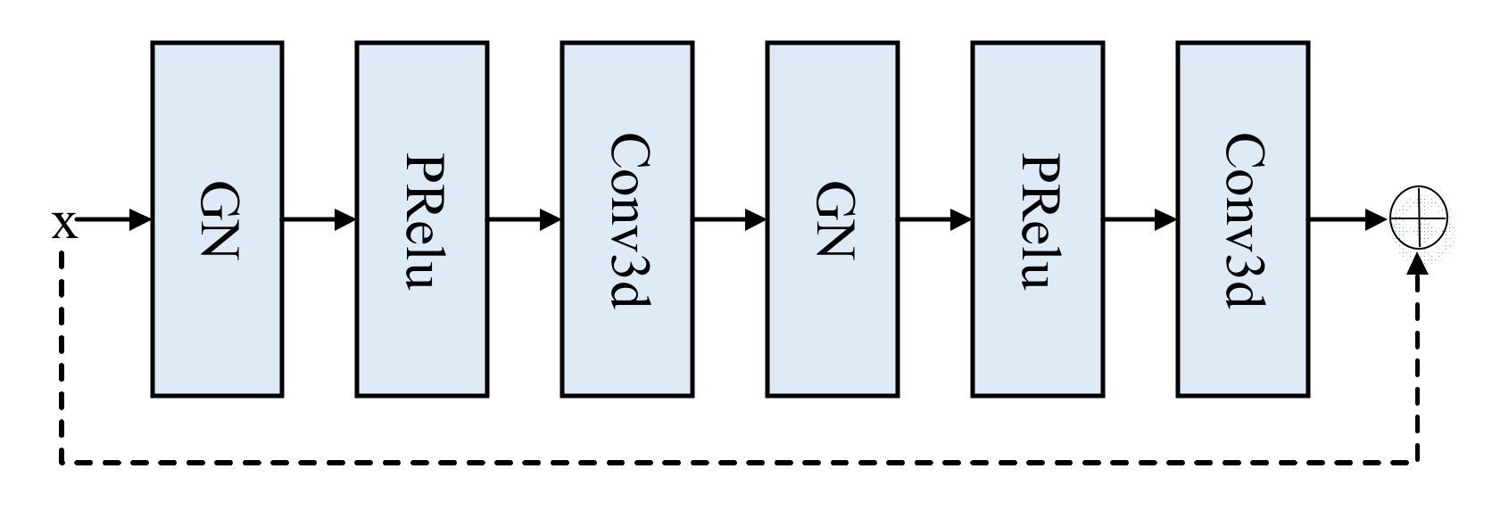
Given that the ordinary convolution loses some characteristic information, a residual basis block method is proposed, consisting of two groups, the normalized group norm and the parametric rectified linear unit (PRelu) [17], and a 3D convolution with a convolution kernel size of 3 and a padding of 1. The structure is displayed in Figure 2.
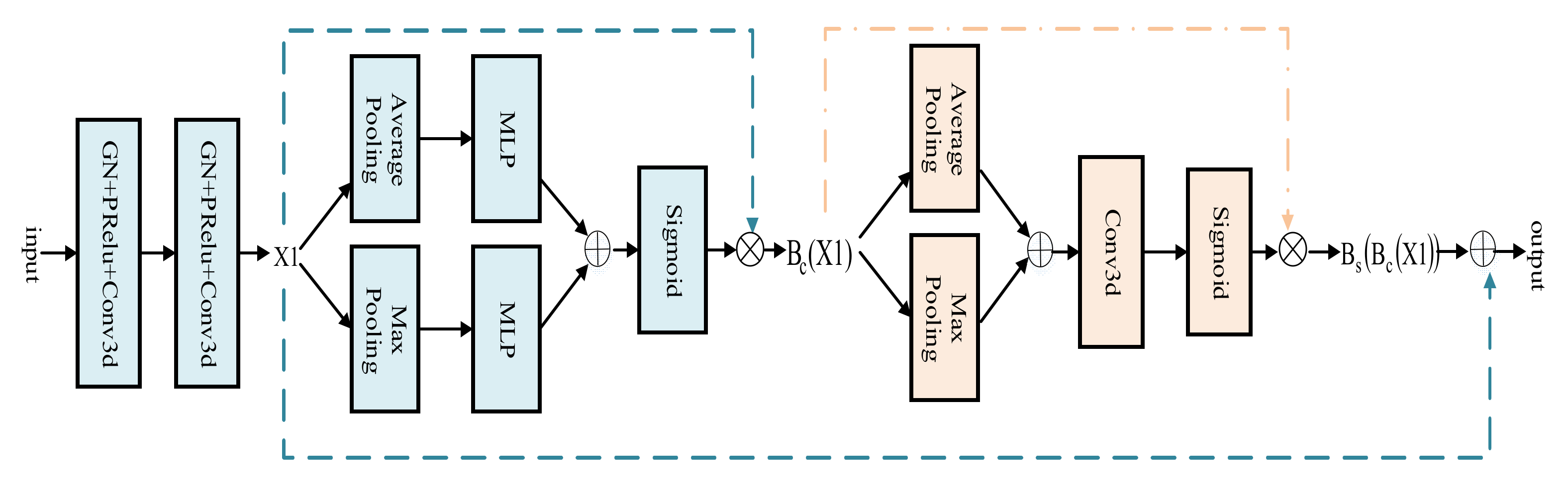
The attention mechanism can selectively assign different weight values to each component, based on the importance of the target region [18]. Therefore, a 3D BCS hybrid domain attention mechanism module is applied to the encoder process. The featured image first enters the CAM and is calculated as shown in Equation (1). Among them, the multilayer perceptron (MLP) is composed of the flatten leveling operation, the linear layer, the reasonable satisfaction linear units (Relu), and the linear layer. Avgpool and MaxPool are abbreviations for the average pooling and maximum pooling, respectively. The joint use of the average and maximum pooling images for more representative spatial information highlights the central information regions.
Following this, it moves on to the SAM, calculated as shown in Equation (2), further compressing the channels to focus on the feature importance of each pixel and extracting the critical information about the image.
The original feature image and the feature image obtained by the hybrid attention mechanism are connected by residuals, as shown in Equation (3), which integrates the weights of the pixels in the different channels and locations of the same track. The 3D downsampling part of the standard U-Net model is extended to maximize the extraction of the original features and to reduce the information loss while increasing the depth of the network.
The architecture of the 3D BCS hybrid domain attention mechanism module is shown in Figure 3.
The input image first goes through the convolution operation with a kernel size of 3, step size of 2, padding of 1, and the image size becomes half of the original. Following the convolution operation, the convolution kernel size is 3, the step is 1, the padding is 1, and the feature graph X1 is obtained. Then, the feature image X1 relates to the residual after the operation of the CAM and the SAM modules to obtain a new feature image for the adaptive optimization.
Compared with the original TransBTS model, the total number of parameters increases from 16.79 MB to 17.99 MB, which can improve the feature extraction capability of the network model without significantly increasing the computation and number of parameters.
3.1.2. Mixed Loss Functions
In brain tumor segmentation, tumor pixel points represent only a tiny fraction of the scanned MRI image. During network training, the predicted values are more likely to favor the background region and ignore the foreground target region, which usually leads to small target segmentation. In previous studies, using a single loss function has not worked well for small target segmentation. Therefore, it is worthwhile to design a hybrid loss function, which is a fusion of the weighted cross-entropy loss (WCE) and the generalized Dice loss (GDL) [19]. The WCE easily achieves the maximum optimization in the backpropagation and focuses on the gradient optimization as Equation (4). Among them, The weight w attributed to the target class can be used to adjust for false positives and false negatives, which can enable an increase in the weight of misclassification and penalizing categories that account for the majority.
The notations are described in Table 2 below.
The GDL considers information on the weights of all classes of brain tumors, focusing on ensuring training stability in the presence of classification imbalances and as Equation (6), using an index as a quantitative indicator of segmentation results.
In practice, the combination of the above two, as shown in Equation (8), enhances the accuracy of the segmentation of small targets and improves the problem of extreme imbalance in the brain tumor category.
3.2. Multimodal Fusion on MRI Data
3.2.1. MRI Datasets
According to the previous description, the BraTS2021 is much larger than the BraTS2020. It is found that it is scientific to adopt the latest BraTS2021 data set, which contains 1251 cases of training data and 219 cases of validation data [20,21,22]. First, we randomly divided the datasets in a ratio of 9:1 to 1126 cases for the model training and 125 points for the model testing and evaluation. The training and test sets are then augmented with data from the training set. This is because we consider that the same sample data may appear in the training and test sets, which will not be scientific enough to characterize the model accurately.
Because the data we used are obtained by MRI scanning, the MRI also obtains information in the clinical environment, but the output size of different devices is different, the pre-training operations such as the normalization and the N4 correction need to be carried out. In addition, the model obtained after training can be used to predict the MRI data without the GT.
As shown in Table 3, the training set underwent four data enhancement methods before being fed into the network model for training. The data images were effectively extended and were sufficiently different from those in the test set. Therefore, it can generalize better than other tumor categories of different patients with some generalization ability.
Each issue contains four modalities, FLAIR, T1, T1ce, and T2, and the image size of each modality is 240 × 240 × 155, representing the length, width, and depth of the voxel block, respectively. Observing the image shows that the effective pixels and tumor area are located in the center of the image. In contrast, the surrounding area is an outside background area. Therefore, the actual area to be processed is the area with the center as the origin and spreading outward. The largest voxel block, 224 × 224 × 128, is used as the model input to maximize the inclusion of the brain contour information. In addition, an N4 bias field correction algorithm has been applied to each modality to compensate for the artifacts in response to problems such as noise interference in the MRI during transmission, resulting in varying intensities of different magnetic field distributions [23].
3.2.2. Data Enhancement
Because the problem of overfitting may occur in the model training for sparse medical images, the issue of insufficient data volume is solved by using the data enhancement method in the training process. There are two kinds of data enhancement, one is the traditional primary image geometric processing method, and the other is the photometric conversion. Considering that the random dropout is used in the training process of the network model, mixing the different modal data of different patients has little significance for the overall training. Therefore, we no longer use the mixed image crossover and randomly erase operations in the photometric transformation, but instead, we use the Gaussian noise operation in the photometric intensity transformation. We mainly use elastic deformation, mirror flip, and the random intensity displacement operations [24].
Specifically, firstly, the image dataset is enhanced by introducing the Gaussian additive noise following the normal distribution on the image to improve the robustness of the network against noise attacks. Secondly, an augmentation method of the elastic deformation is used to simulate the difference of different shapes to solve the irregular and discontinuous boundary problem of tumors in medical images. Since the model image is independent of the position direction, the inverted image is equivalent to the new data of the same category, so the mirror inversion with the probability of turning the axial, the coronal and the sagittal planes of 0.5 is used to increase the data sample. In addition, the random intensity shift operation achieves the effect of the sample expansion by applying an intensity shift in the scale factor range of [−0.1, 0.1] and a scaling in the scale range of [0.9, 1.1]. This way, the scale from 1 to 4 is expanded by four data enhancement methods, increasing the data set’s randomness and giving the model a better generalization ability.
4. Experimental Results and Analysis
4.1. Experimental Environment and Evaluation Indicators
The experimental platform is a Linux operating system; the simulation tools are the Pycharm framework, the Pytorch environment, and the CUDA 10.2 architecture platform. All training and experiments are run on a standard workstation (dual Intel(R) Xeon(R) Gold 5218 CPUs, Tesla V100×4 graphics card, 256 GB RAM).
The image results are evaluated using the classical Dice similarity coefficient (DSC), the Hausdorff 95 (HD95), and sensitivity [23]. The values of the DSC and sensitivity range from 0 to 100%, with higher scores indicating a better segmentation accuracy. HD95 means how close the actual value is to the predicted value and is inversely proportional to the segmentation result, with lower values showing better segmentation results.
4.2. Analysis of the Ablation Experiments
The experiments are conducted using uniform experimental environment parameters to verify the effectiveness of the added modules on the overall model. Considering that the anthropomorphic Newton method (Apollo) can dynamically apply the curvature of the loss function to the optimization [25], the Apollo optimizer is used in the training process of this paper. In the early stage of the experiment, several hyperparameters in the experiment, including the learning rate and batch size, were dynamically adjusted through multiple rounds of cross-validation to obtain the optimal value through the manual experience adjustment and considering the problem of memory capacity. Finally, the batch size was set as four, and the learning rate as 0.0002.
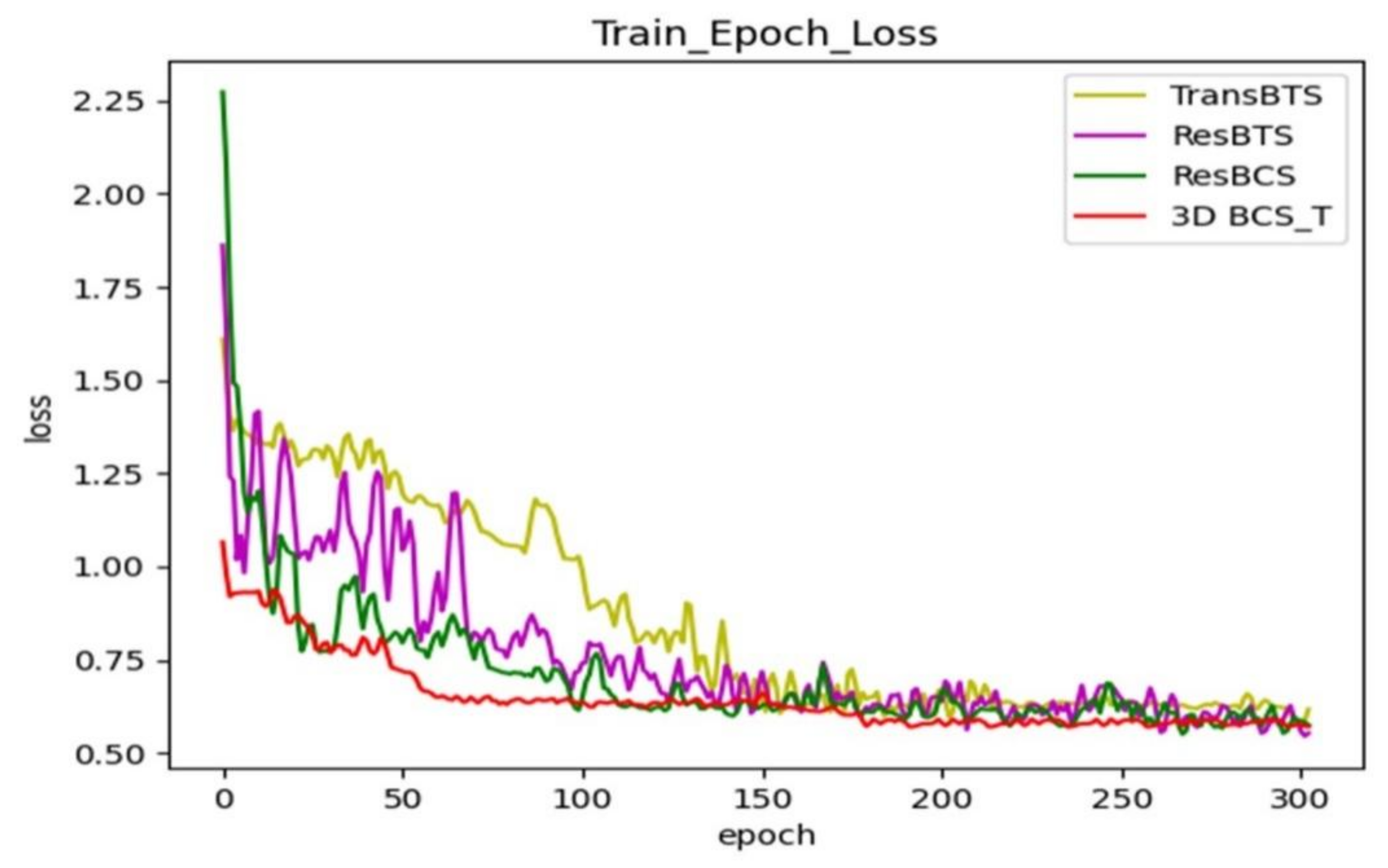
The modules are renamed to facilitate the subsequent viewing of the results. The ResBTS network represents adding a new layer of network depth to the original model and the residual-based block convolution. The ResBTS network consists of a new layer of the network depth added to the original model and the residual-based block convolution. The ResBCS network forms by adding the 3D BCS hybrid attention mechanism module to the ResBTS network. The 3D BCS_T model replaces the single loss function of the ResBCS network using a fused loss function of the WCE and the GDL.
Figure 4 shows the comparison of the loss function during training after adding each module; each curve represents a different network model. Our final model keeps the loss in the training phase at around 0.6 after adding the hybrid loss function, which has a better generalization ability.
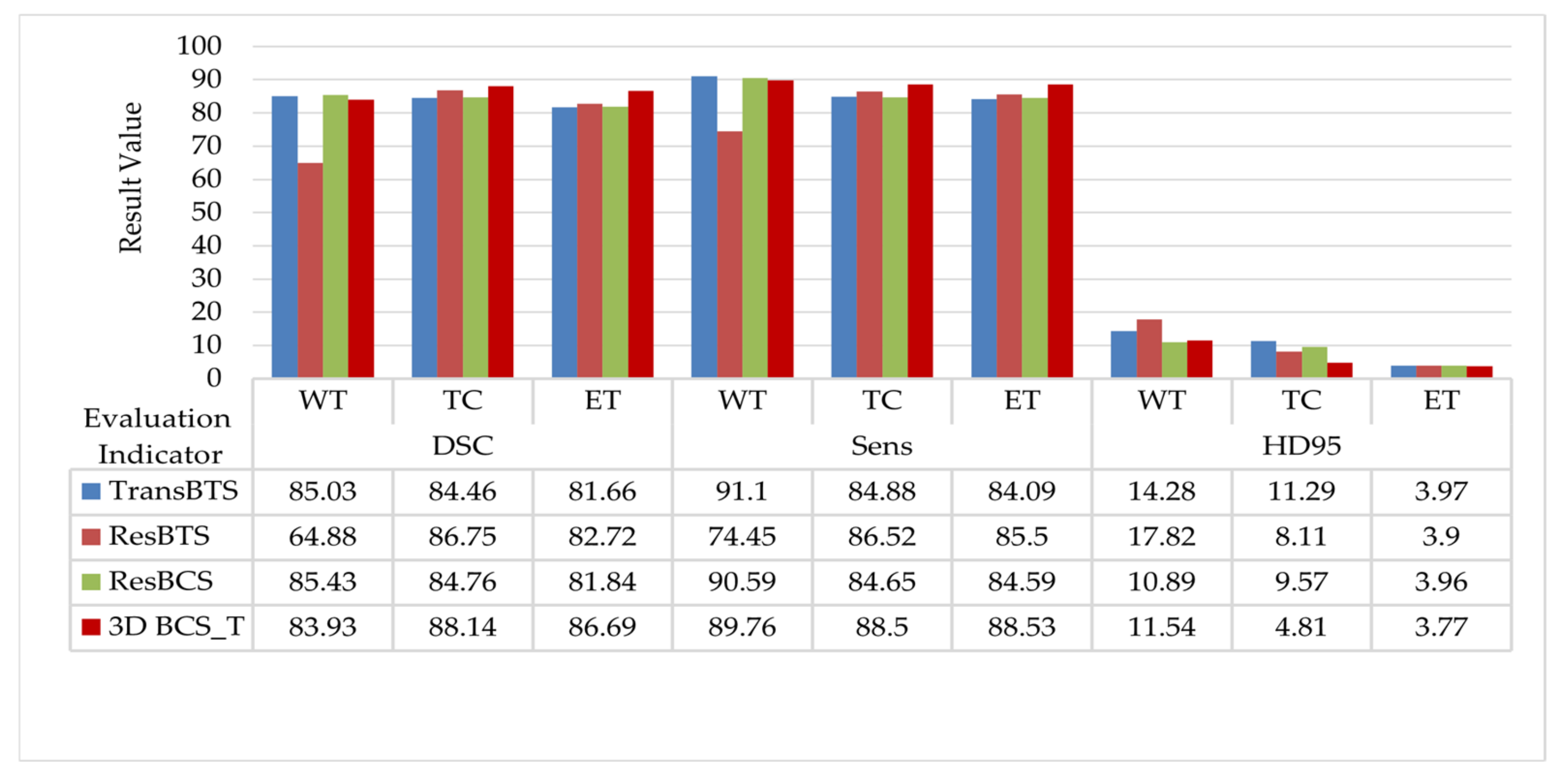
The quantitative data evaluated in the test set are shown in Figure 5. The ResBTS network improved the DSC in the TC and ET regions by 2.29% and 1.06%, respectively, compared to the original model. The ResBCS network, allowing attention to be focused on the target region, improves the Sens metric in correctly segmenting the tumor compared to the original model. Furthermore, the hybrid loss function is used further to improve the DSC of the TC and ET regions. The HD95 distance is further reduced, which is more friendly to small area segmentation.
The model is trained in 300 rounds, each round takes about 21 min to train and the test time is about 1 s. When the model is well trained, it can be used directly for image segmentation without the need to repeat the training. The method used in this paper can achieve image input to segmentation in less than 3 s, with a relatively fast response.
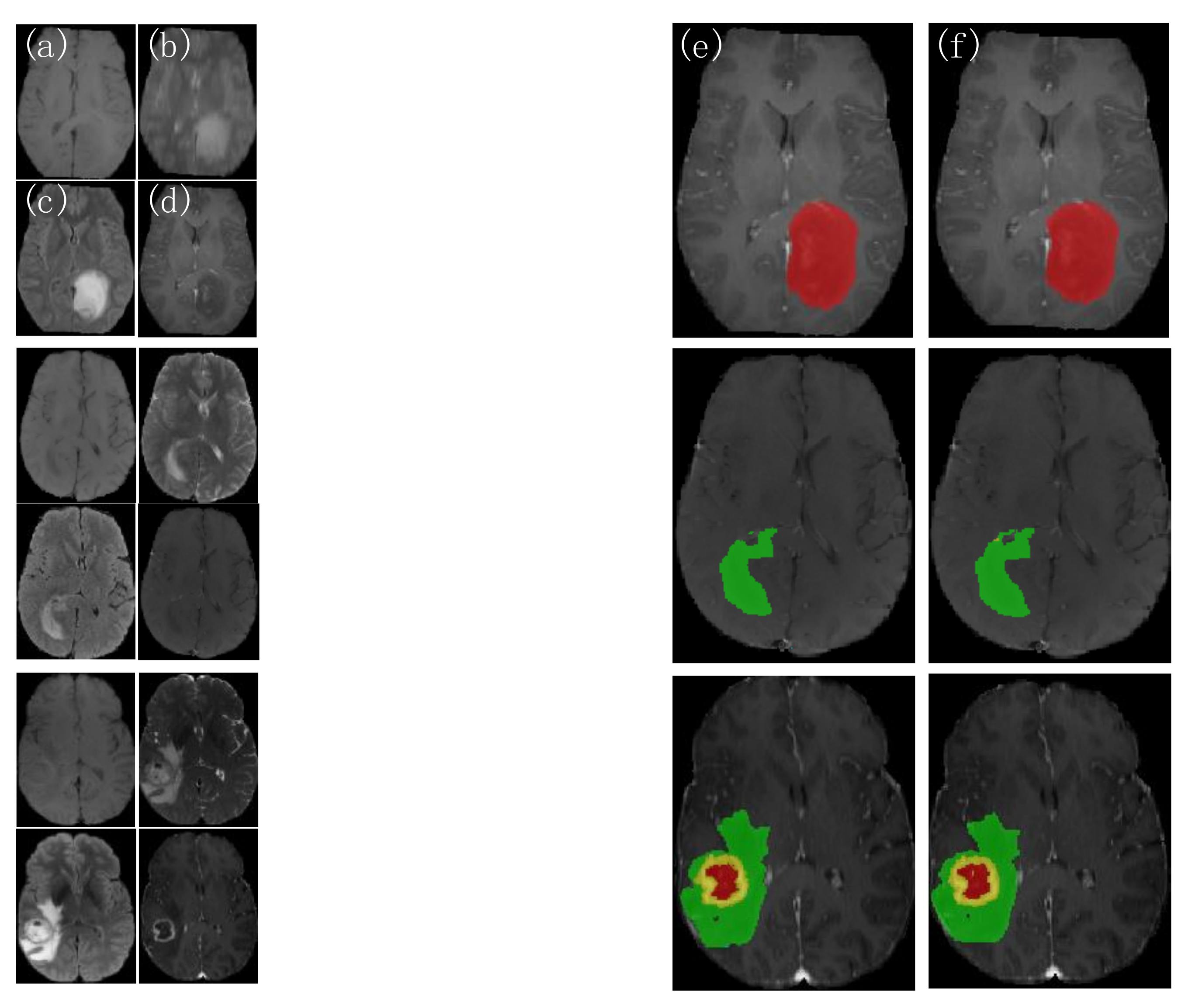
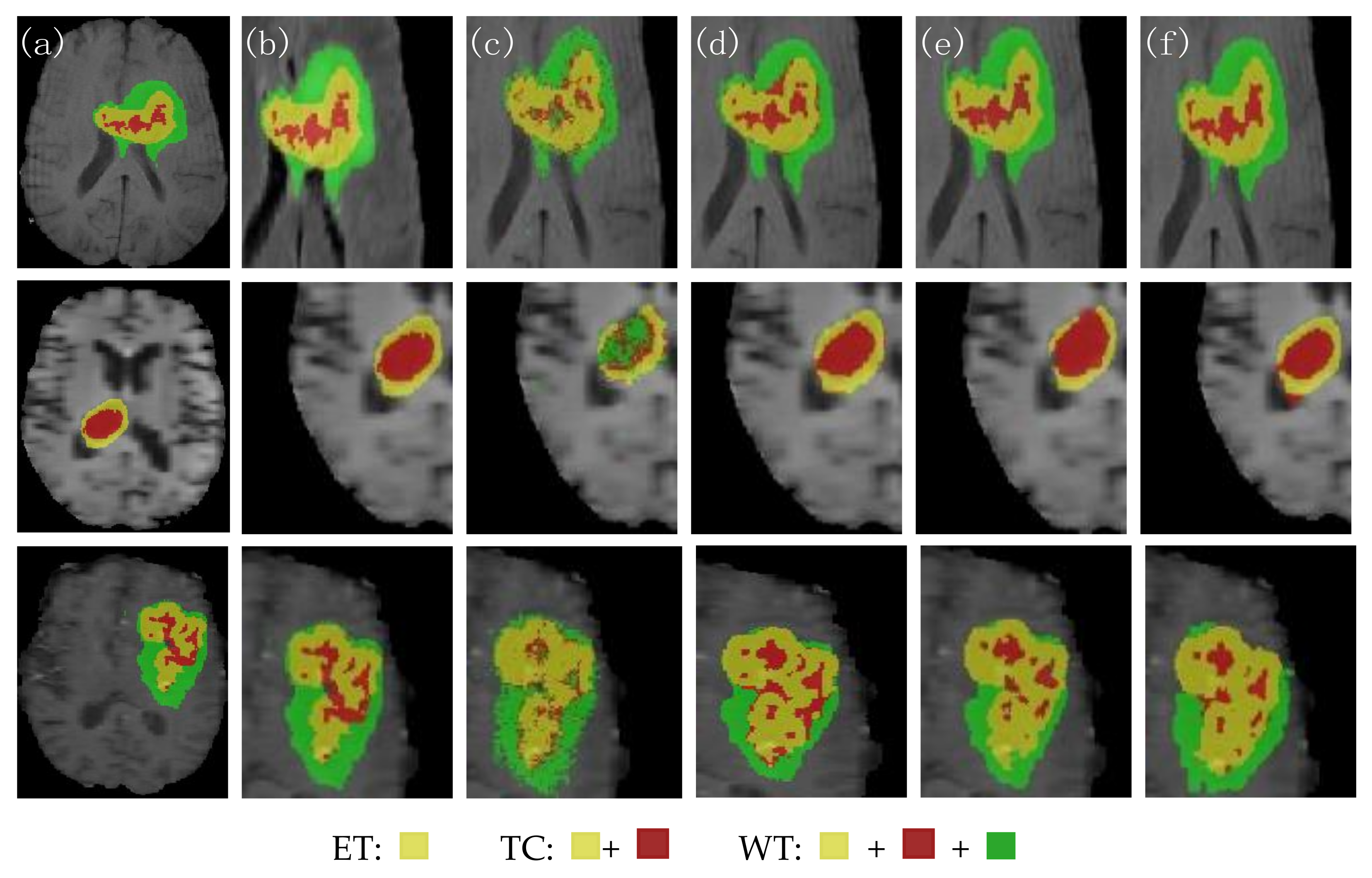
Three groups of patient images are randomly selected from the test set, as shown in Figure 6. The picture on the left shows each of the four modalities of the MRI images, and on the other side represents from left to right, the 3D BCS_T model predicted outcome image and the expert-labeled ground truth(GT). The first two groups of patients have only single-category tumor regions (the first group has only gangrenous NET areas and the second group has only puffy ED regions). In contrast, the last group has three categories of parts: WT, TC, and ET. The different areas have additional individual variability, with shape and size characteristics showing their regional features, making the segmentation task more difficult.
As shown in the results, the 3D BCS_T model can segment the target region more accurately when facing different segmentation region types, effectively overcoming the variability of variable region types and accurately segmenting the contours of the enhanced tumor and tumor core. The model has a strong robustness and adaptability, with the solid network performance.
4.3. Analysis of the Comparative Experiments
The 3D BCS_T network is compared with other convolutional neural networks to verify the effectiveness of the improved method. The 3D Unet and the convolutional block attention module (CBAM) Unet are four-layer encoder-decoder U-shaped structures [7]. Still, given that the maximum pooling used in the original model for the downsampling and the trilinear interpolation used for the upsampling lose some information, the network is further improved and refined. On the one side, the expansion convolution replaces the maximum pooling, which contains a convolution kernel size of 3, a step size of 2, a fill of 2, and a dilation rate of 2. On the other side, the transposed convolution replaces the linear interpolation. Finally, to ensure the stability of the training, the random discard dropout is set to 0.3. The model is trained 300 rounds from scratch, using a five-fold cross-validation. The segmentation results of the validation set are evaluated for 226 cases, and the DSC results are shown in Table 4. The DSC of the network with the attention mechanism added improved by 8.8% over the original network model.
4.3.1. Analysis of the Visualization Results
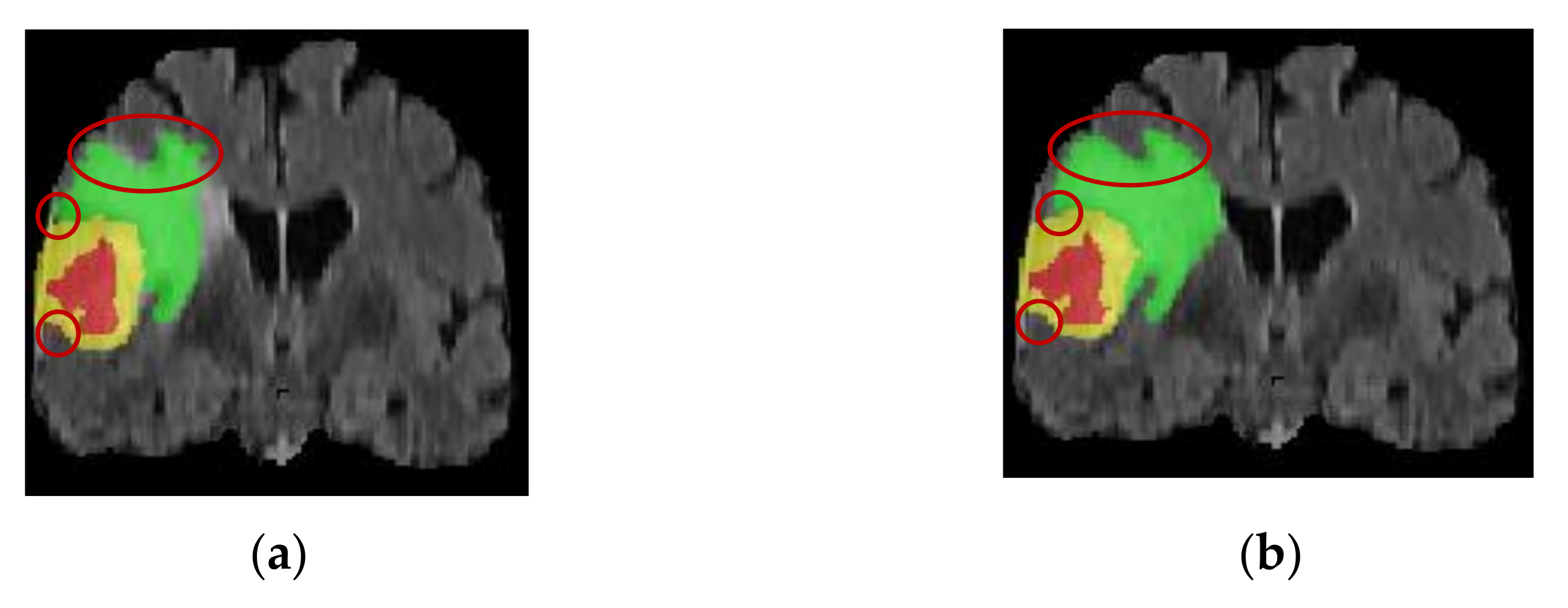
Two patient images are randomly selected to visualize the difference in the segmentation results before and after the improvement of the network model. The patient in Figure 7 had irregularly shaped tumor regions with irregular edges and small lesion regions with a severe class imbalance. The TransBTS model is not fine enough in segmentation for the small target processing and has incorrect prediction labels. In contrast, the improved model has advantages for small target segmentation and obtains accurate edge information. This indicates that the 3D BCS_T model can effectively solve the problems caused by the irregular shape of the tumor region, improve the segmentation effect and edge segmentation accuracy of the smaller lesion regions, and has a strong adaptability.
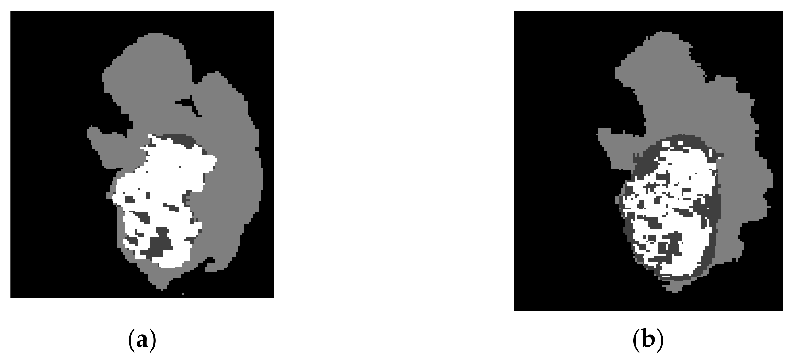
The patient image in Figure 8 has a non-uniform greyscale, a discontinuous distribution of tumor structures, and many outliers and noises. At the same time, the TransBTS model tends to miss or misjudge the discrete tumor pixels. The 3D BCS_T model, however, is more stable and robust by designing a residual join and a jump join operation to linearly combine the residual processed information with the original input information to obtain more local feature information, eliminating irrelevant and noisy features.
4.3.2. Analysis of the Datasets Results
The segmentation results of the test set on different network models are shown in Table 5. Following the triple-fold cross validation, the mean value of the three-class tumor segmentation DSC using the classical 3D Unet network is 73.69. The CBAM Unet network, with the addition of the hybrid attention mechanism, has a tumor segmentation DSC of up to 82.49, which further demonstrates the effectiveness of adding the attention module to the overall network. In addition, the 3D Unet network and the CBAM Unet network have larger values for the HD95 distance due to the random division of the data in the test set of this experiment and the uneven distribution of the tumor target regions, where a very small pixel segmentation results in a larger oscillation distance.
Compared with the original TransBTS network, the DSC of the 3D BCS_T network on the WT, TC, and ET are 83.93, 88.14, and 86.69, respectively. The average values of the TC and ET are increased by 3.68% and 5.03%, respectively, compared with the suboptimal model. It shows that the 3D BCS_T algorithm model performs better in segmenting tumor core areas and enhanced areas and can significantly improve the segmentation performance of small-scale tumors. The model has significant advantages over other models in various performance indicators. Overall, combining our proposed residual basis block, the 3D BCS hybrid domain attention mechanism, and the hybrid loss function can improve the boundary clarity of the DSC and tumor segmentation and reduce the HD95 distance.
At the same time, we can notice that the DSC of the WT area is not ideal, mainly because the prediction number of tag 2 in the swollen area is relatively inaccurate, which leads to the prediction result of the WT category not achieving the best effect. However, compared with other models, this model has apparent advantages in the DSC, Sens, and HD95 distance performance indexes.
Following the 6-fold cross-validation and averaging, the resultant values of the DSC on the WT, TC, and ET category tumors are 83.96, 88.15, and 86.70, respectively, proving that our network remained stable and effective in the tumor segmentation results.
Figure 9 shows the visual segmentation results of the three groups of patients randomly selected. From left to right, they are the expert manually annotated GT, the local expansion image, the 3D Unet segmentation result image, the CBAM Unet segmentation result image, the TransBTS segmentation result image, and the 3D BCS_T segmentation result image. The morphology and size of the MRI in the three groups were different. The edge of the tumor area in the first group was irregular. The lesion area in the second group was small. Moreover, the tumor distribution in the third group was discontinuous, with more outliers and noise. No matter the contrast and noise of the original image, the 3D BCS_T network has the best effect in predicting the enhanced tumors and core tumors. Among them, the DSC of the second group of patients is 91.01, 96.67, and 91.70 in the WT, TC, and ET, respectively. The patient has only enhanced tumors and edema areas, and the prediction results of this model are almost the same as those of the GT.
Combining the statistics in Table 3 and the above discussion, we can conclude that the 3D Unet has significant problems in pixel fine-grained segmentation, and the CBAM Unet misclassifies the background regions as the ET regions in some segmentation results. The 3D Unet has significant issues in pixel fine-grained segmentation, with the CBAM Unet misclassifying the background regions as the ET regions in some segmentation results. The TransBTS is not accurate enough in segmenting region contours, especially the blurred inner edges. Our proposed 3D BCS_T model has the following advantages:
- The 3D BCS hybrid domain attention mechanism module helps to improve the model’s recognition of the important feature information, and the residual connectivity enhances the segmentation ability. The hybrid loss function can further improve the segmentation accuracy of small targets and optimize the network performance.
- Our model has a low average deviation and a low dispersion, which allows for the further segmentation of the detailed contour of the model.
- In terms of the edge determination and accuracy of the ET and TC tumor areas, the model is superior to other SOTA models, which can help doctors accurately determine the precise location of the incision in surgery and protect patients’ healthy tissues from being removed.
5. Conclusions
To further improve the accuracy of tumor segmentation and the clarity of regional contours, an improved 3D BCS_T segmentation network is proposed based on the original TransBTS model, which retains the underlying features of the transformer, and introduces a residual basis block. A 3D BCS hybrid domain attention mechanism to fully use the information features from different levels of the encoder and decoder, and finally, a hybrid loss function is proposed to train the network model adequately. Experimental results on the BraTS2021 dataset show that the improved network achieves the best results in all three evaluation metrics in the ET and TC regions, proving the improved method’s worthiness.
However, this work also has certain limitations. On the one hand, increasing the depth of the network model leads to an increase in the number of parameters and a longer training time. Next, we will consider how to improve the time to reduce the number of parameters and complexity while improving the accuracy. On the other hand, the effectiveness of the proposed method is only demonstrated in the segmentation task of brain tumor MRI images with four modes. In the subsequent work, the network will be adjusted to accept other modality format datasets of the MRI as the model’s input to be widely used in medical image segmentation and reduce some burden for doctors.
Author Contributions
Conceptualization, X.C.; methodology, X.L. and X.C.; software, and validation, X.L.; formal analysis and investigation, X.C.; resources, data curation, and writing—original draft preparation, X.L.; writing—review and editing, X.C. All authors have read and agreed to the published version of the manuscript.
Funding
This research received no external funding.
Institutional Review Board Statement
Not applicable.
Informed Consent Statement
Not applicable.
Data Availability Statement
The dataset supporting the conclusions of this article are available at https://www.synapse.org/#!Synapse:syn27046444/wiki/616571, accessed on 10 July 2022.
Conflicts of Interest
The authors declare no conflict of interest.
Abbreviations
| MRI | Magnetic resonance imaging |
| T1 | T1-weighted imaging |
| T2 | T2-weighted imaging |
| FLAIR | Fluid attenuated inversion Recovery |
| T1ce | T1-weighted imaging with contrast medium |
| CNN | Convolutional neural network |
| MRFCM | Modified robust fuzzy c-means |
| PRelu | Parametric rectified linear unit |
| MLP | Multilayer perceptron |
| Relu | Reasonable satisfaction linear units |
| WCE | Weighted cross-entropy loss |
| GDL | Generalized Dice loss |
| DSC | Dice similarity coefficient |
| HD95 | Hausdorff 95 |
| CBAM | Convolutional block attention module |
| GT | Ground truth |
References
- Louis, D.N.; Perry, A.; Wesseling, P.; Brat, D.J.; Cree, I.A.; Figarella-Branger, D.; Hawkins, C.; Ng, H.K.; Pfister, S.M.; Reifenberger, G.; et al. The 2021 WHO Classification of Tumors of the Central Nervous System: A summary. Neuro Oncol. 2021, 23, 1231–1251. [Google Scholar] [CrossRef] [PubMed]
- Li, H.Z.; Wu, Y.B.; Sun, W.D.; Guo, Z.Y.; Xie, J.J. Design and implement low field magnetic resonance main Magnet based on Halbach structure. J. Instrum. 2022, 43, 46–56. [Google Scholar]
- He, C.E.; Xu, H.J.; Wang, Z.; Ma, L.P. Automatic segmentation of brain tumor images by multimodal magnetic resonance imaging. Acta Opt. Sin. 2020, 40, 66–75. [Google Scholar]
- Kamnitsas, K.; Ledig, C.; Newcombe, V.F.; Simpson, J.P.; Kane, A.D.; Menon, D.K.; Rueckert, D.; Glocker, B. Efficient multi-scale 3D CNN with fully connected CRF for accurate brain lesion segmentation. Med. Image Anal. 2017, 36, 61–78. [Google Scholar] [CrossRef] [PubMed]
- Song, J.H.; Zhang, Z. A Modified Robust FCM Model with Spatial Constraints for Brain MR Image Segmentation. Information 2019, 10, 74. [Google Scholar] [CrossRef]
- Dvořák, P.; Menze, B. Local Structure Prediction with Convolutional Neural Networks for Multimodal Brain Tumor Segmentation. In Proceedings of the International MICCAI Workshop on Medical Computer Vision, Medical Computer Vision: Algorithms for Big Data, Cham, Switzerland, 1 July 2016; pp. 59–71. [Google Scholar]
- Henry, T.; Carré, A.; Lerousseau, M.; Estienne, T.; Robert, C.; Paragios, N.; Deutsch, E. Brain tumor segmentation with self-ensembled, deep-ly-supervised 3D U-net neural networks: A BraTS 2020 challenge solution. arXiv 2020, arXiv:2011.01045. [Google Scholar]
- Dosovitskiy, A.; Beyer, L.; Kolesnikov, A.; Weissenborn, D.; Zhai, X.H.; Unterthiner, T.; Dehghani, M.; Minderer, M.; Heigold, G.; Gelly, S.; et al. An Image is Worth 16x16 Words: Transformers for Image Recognition at Scale. arXiv 2020, arXiv:2010.11929. [Google Scholar]
- Chen, J.N.; Lu, Y.L.; Yu, Q.H.; Luo, X.D.; Adeli, E.; Wang, Y.; Lu, L.; Yuille, A.L.; Zhou, Y.Y. TransUNet: Transformers Make Strong Encoders for Medical Image Segmentation. arXiv 2021, arXiv:2102. 04306. [Google Scholar]
- Wang, W.X.; Chen, C.; Ding, M.; Li, J.Y.; Yu, H.; Zha, S. TransBTS: Multimodal Brain Tumor Segmentation Using Transformer. arXiv 2021, arXiv:2103. 04430. [Google Scholar]
- Chen, H.; Dou, Q.; Yu, L.; Qin, J.; Heng, P.A. VoxResNet: Deep voxelwise residual networks for brain segmentation from 3D MR images. Neuroimage 2018, 170, 446–455. [Google Scholar] [CrossRef]
- Hou, F.Z.; Zou, B.J.; Liu, Z.B.; Zhou, Z.Y. Multi-modal brain MR image tumor segmentation algorithm based on gray distribution matching. Appl. Res. Comput. 2017, 34, 3869–3872. [Google Scholar]
- Chu, J.H.; Li, X.C.; Zhang, J.Q.; Lv, W. Fine segmentation of 3d brain tumor based on cascade convolution network. Laser Optoelectron. Prog. 2019, 56, 75–84. [Google Scholar]
- Ge, T.; Zhan, T.M.; Mou, S.X. Brain tumor segmentation algorithm based on multi-core synergy said classification. J. Nanjing Univ. Sci. Technol. Lancet 2019, 43, 578–585. [Google Scholar]
- Feng, Y.; Li, J.; Zhang, X. Research on Segmentation of Brain Tumor in MRI Image Based on Convolutional Neural Network. BioMed Res. Int. 2022, 2022, 7911801. [Google Scholar] [CrossRef]
- Jia, Q.; Shu, H. BiTr-Unet: A CNN-Transformer Combined Network for MRI Brain Tumor Segmentation. In Brainlesion Glioma, Multiple Sclerosis, Stroke and Traumatic Brain Injuries. BrainLes (Workshop); Springer: Cham, Switzerland, 2021; pp. 3–14. [Google Scholar]
- Hu, G.D.; Qian, F.Y.; Sha, L.G.; Wei, Z.L. Application of Deep Learning Technology in Glioma. J. Healthc Eng. 2022, 2022, 8507773. [Google Scholar] [CrossRef]
- Woo, S.; Park, J.; Lee, J.; Kweon, I.S. CBAM: Convolutional Block Attention Module. arXiv 2018, arXiv:1807.06521. [Google Scholar]
- Sudre, C.H.; Li, W.Q.; Vercauteren, T.; Ourselin, S.; Cardoso, M.J. Generalised Dice overlap as a deep learning loss function for highly unbalanced segmentations. arXiv 2017, arXiv:1707.03237. [Google Scholar]
- Menze, B.H.; Jakab, A.; Bauer, S.; Kalpathy-Cramer, J.; Farahani, K.; Kirby, J. The Multimodal Brain Tumor Image Segmentation Benchmark (BRATS). IEEE Trans. Med. Imaging 2015, 34, 1993–2024. [Google Scholar] [CrossRef]
- Bakas, S.; Akbari, H.; Sotiras, A.; Bilello, M.; Rozycki, M.; Kirby, J.S.; Freymann, J.B.; Farahani, K.; Davatzikos, C. Advancing the Cancer Genome Atlas glioma MRI collections with expert segmentation labels and radiomic features. Nat. Sci. Data 2017, 4, 170117. [Google Scholar] [CrossRef]
- Baid, U.; Chodasara, S.; Mohan, S.; Bilello, M.; Calabrese, E.; Colak, E.; Farahani, K. The RSNA-ASNR-MICCAI BraTS 2021 Benchmark on Brain Tumor Segmentation and Radiogenomic Classification. arXiv 2021, arXiv:2107.02314. [Google Scholar]
- Kaur, G.; Rana, P.S.; Arora, V. State-of-the-art techniques using pre-operative brain MRI scans for survival prediction of glioblastoma multiforme patients and future research directions. Clin. Transl. Imaging 2022, 3, 355–389. [Google Scholar] [CrossRef]
- Adaloglou, M.N. Deep Learning in Medical Image Analysis: A Comparative Analysis of Multi-Modal Brain-MRI Segmentation with 3D Deep Neural Networks. Master’s Thesis, University of Patras, Patra, Greece, 2019. [Google Scholar]
- Ma, X.Z. Apollo: An Adaptive Parameter-wise Diagonal Quasi-Newton Method for Nonconvex Stochastic Optimization. arXiv 2020, arXiv:2009.13586. [Google Scholar]
Figure 1.
3D BCS_T network model structure. The left side represents the encoder and decoder parts of the U-network, while the right side represents the self-encoder part of the Vision Transformer. Abbreviations: the channel attention module (CAM), the spatial attention module (SAM), positional encoding (PE). Furthermore, Conv3d represents a convolution operation with a convolution kernel size of 2 and a step size of 2.

Figure 2.
Residual base block structure.

Figure 3.
3D BCS Hybrid Domain Attention Mechanism Module.

Figure 4.
Comparison of the training loss functions with the different modules added to the TransBTS network.
Figure 4.
Comparison of the training loss functions with the different modules added to the TransBTS network.

Figure 5.
Comparison of the evaluation results with the different modules added to the TransBTS network.
Figure 5.
Comparison of the evaluation results with the different modules added to the TransBTS network.

Figure 6.
Comparison of the actual segmentation of the 3D BCS_T model tumors in different patients. (a) T1 images; (b) T2 images; (c) FLAIR images; (d) T1ce images; (e) 3D BCS_T images; (f) GT images.
Figure 6.
Comparison of the actual segmentation of the 3D BCS_T model tumors in different patients. (a) T1 images; (b) T2 images; (c) FLAIR images; (d) T1ce images; (e) 3D BCS_T images; (f) GT images.

Figure 7.
Comparison of the sagittal bit image segmentation results. (a) Pre-improvement segmentation; (b) Post-improvement segmentation.
Figure 7.
Comparison of the sagittal bit image segmentation results. (a) Pre-improvement segmentation; (b) Post-improvement segmentation.

Figure 8.
Comparison of the greyscale image segmentation results. (a) Pre-improvement segmentation; (b) Post-improvement segmentation.
Figure 8.
Comparison of the greyscale image segmentation results. (a) Pre-improvement segmentation; (b) Post-improvement segmentation.

Figure 9.
Comparison of the segmentation effects of the different network models. (a) GT; (b) local expansion; (c) 3D Unet; (d) CBAM Unet; (e) TransBTS; (f) 3D BCS_T; From the perspective of the segmented category area, there were three types of tumors in the first and third groups, namely ET, TC and WT. The second group only had ET and TC tumors.


Table 1.
Review of the techniques and databases used for the brain tumor image segmentation from 2016 to 2022.
Table 1.
Review of the techniques and databases used for the brain tumor image segmentation from 2016 to 2022.
| Paper | Year | Technology | D.V.S | D.E. | R.C | A.M.O | L.F.O |
|---|---|---|---|---|---|---|---|
| [11] | 2016 | VoxResNet | 20 | × | √ | × | × |
| [12] | 2017 | Grayscale indexing match | 50 | × | × | × | × |
| [13] | 2018 | Vnet | 285 | √ | × | × | √ |
| [14] | 2019 | Cooperative representation | 65 | × | × | × | × |
| [7] | 2020 | 3D Unet | 369 | √ | × | √ | × |
| [10] | 2021 | TransBTS | 369 | √ | × | × | × |
| [15] | 2021 | CNN Transformer | 1251 | √ | × | × | × |
| [16] | 2022 | CNN | 65 | × | × | × | × |
| Ours | 2022 | CNN Transformer | 1251 | √ | √ | √ | √ |
Table 2.
Definition of the symbols.
| Symbol | Implication |
|---|---|
| m | Number of categories |
| w | Weighting |
| n | Number of pixel points |
| The actual value of the segmented label graph given by the data | |
| A predicted probability value of a pixel belonging to category j | |
| The actual value of category j at pixel i | |
| A predicted probability value of category j at pixel i |
Table 3.
Experimental data is randomly divided according to the proportion.
| Type | Percentage | Number | Scramble Order | Data Enhancement | Total Number |
|---|---|---|---|---|---|
| Training set | 90 | 1126 | √ | √ | 4504 |
| Test set | 10 | 125 | √ | × | 125 |
Table 4.
Results of the DSC evaluation of the classical networks on the validation set. AVG is the abbreviation for average.
Table 4.
Results of the DSC evaluation of the classical networks on the validation set. AVG is the abbreviation for average.
| Network | DSC (%) | |||
|---|---|---|---|---|
| ET | TC | WT | AVG | |
| 3D Unet | 72.41 | 73.67 | 74.99 | 73.69 |
| CBAM Unet | 80.81 | 82.89 | 83.77 | 82.49 |
Table 5.
Comparison of the evaluation results of the different network models. The underlined data indicate that the network model has the best evaluation result compared with other models under the same evaluation index and category.
Table 5.
Comparison of the evaluation results of the different network models. The underlined data indicate that the network model has the best evaluation result compared with other models under the same evaluation index and category.
| Network | DSC (%) | Sens (%) | HD95 | ||||||
|---|---|---|---|---|---|---|---|---|---|
| WT | TC | ET | WT | TC | ET | WT | TC | ET | |
| 3D Unet | 75.60 | 72.70 | 70.19 | 88.55 | 81.62 | 84.16 | 75.6 | 72.7 | 70.19 |
| CBAM Unet | 85.18 | 81.85 | 78.03 | 90.75 | 86.24 | 85.71 | 25.49 | 8.92 | 8.52 |
| TransBTS | 85.03 | 84.46 | 81.66 | 91.10 | 84.88 | 84.09 | 14.28 | 11.29 | 3.97 |
| 3D BCS_T | 83.93 | 88.14 | 86.69 | 89.76 | 88.50 | 88.53 | 11.54 | 4.81 | 3.77 |
Publisher’s Note: MDPI stays neutral with regard to jurisdictional claims in published maps and institutional affiliations. |
© 2022 by the authors. Licensee MDPI, Basel, Switzerland. This article is an open access article distributed under the terms and conditions of the Creative Commons Attribution (CC BY) license (https://creativecommons.org/licenses/by/4.0/).
Share and Cite
MDPI and ACS Style
Liu, X.; Cheng, X. Segmentation Method of Magnetoelectric Brain Image Based on the Transformer and the CNN. Information 2022, 13, 445. https://doi.org/10.3390/info13100445
AMA Style
Liu X, Cheng X. Segmentation Method of Magnetoelectric Brain Image Based on the Transformer and the CNN. Information. 2022; 13(10):445. https://doi.org/10.3390/info13100445
Chicago/Turabian StyleLiu, Xiaoli, and Xiaorong Cheng. 2022. "Segmentation Method of Magnetoelectric Brain Image Based on the Transformer and the CNN" Information 13, no. 10: 445. https://doi.org/10.3390/info13100445
Note that from the first issue of 2016, this journal uses article numbers instead of page numbers. See further details here.