
Prediction of Enterprise Free Cash Flow Based on a Backpropagation Neural Network Model of the Improved Genetic Algorithm


1
Supervising and Auditing Office, Northeastern University, Qinhuangdao 066004, China
2
School of Computer and Communication Engineering, Northeastern University, Qinhuangdao 066004, China
*
Author to whom correspondence should be addressed.
Information 2022, 13(4), 172; https://doi.org/10.3390/info13040172
Submission received: 17 February 2022
/
Revised: 22 March 2022
/
Accepted: 28 March 2022
/
Published: 29 March 2022
Abstract
:Enterprises with good long-term free cash flow data often have better prospects than enterprises with good net profit but unstable free cash flow for a long time, and free cash flow prediction is an important part of evaluating the enterprise value of an enterprise. By determining the fitness function, algorithm formula, population, and Backpropagation (BP) neural network design, a BP neural network model based on the improved genetic algorithm is proposed to predict the free cash flow of enterprises. Taking the free cash flow data of G Company from 1 January 2019 to 30 June 2019 as an example, after evaluating the most neurons and the best population, analyzing the relative errors and comparing the average relative errors of different prediction models, the results show that the model has better prediction accuracy. Cash flow forecasting can effectively improve decision making on productions and operations and the investment financing of enterprises, and has important practical significance for studying enterprise fund management.
1. Introduction
As an important indicator to measure the future sustainable management ability of enterprises, enterprise value can provide important decision-making information for stakeholders and help to identify enterprises with good prospects [1,2,3,4,5,6,7]. At present, enterprise valuation methods mainly include the income method, cost method, and market method, among which the free cash flow discount method is the most widely used [8]. Free cash flow is the remaining cash flow after meeting the needs of business activities and reinvestment, and is the discretionary cash obtained by enterprises [9,10,11,12]. The discounted free cash flow method is used to evaluate enterprise value, which includes three steps: predicting the performance and free cash flow, estimating the discount rate, and estimating the continuous value. When forecasting free cash flow, choosing a scientific and reasonable method is an important prerequisite for accurately evaluating enterprise value [13,14,15,16,17,18,19,20].
In past research, the time series forecasting method has been the main method used to forecast free cash flow, including the grey model [21], Markov model [22], neural network [23], BP neural network [24], and so on, but each method has its own applicable conditions and limitations. Luo et al. [21] used the improved grey prediction method as an absolute valuation model to estimate cash flow. Yao et al. [22] provided a general model to investigate stochastic cash flows in both wealth and liability dynamic processes using Markov chain. Rowland et al. [23] presented a methodology based on neural networks that takes into consideration seasonal fluctuations when equalizing time series, using the Czech crown and Chinese yuan as examples. Li et al. [24] proposed a method for predicting using a BP neural network. In addition, there are several other models [25,26,27,28,29,30]. Jennergren [25] focused on continuing value with the discounted cash flow model. Décamps et al. [26] developed a dynamic model of a firm facing agency costs of free cash flow. Tabei et al. [27] proposed a new method for forecasting projected cash flow under a fuzzy environment. Weytjens et al. [28] predicted accounts receivable cash flows by employing methods applicable to companies with many customers and transactions. Hsu [29] attempted to innovate by deploying a model of time series prediction for e-commerce cash flow service customers. Wang and Ning [30] proposed a hybrid learning algorithm based on the adaptive population activity particle swarm optimization algorithm combined with the least squares method to optimize the adaptive network-based fuzzy inference system model parameters.
In terms of the prediction effect, because a BP neural network is a multilayer feedforward neural network trained according to the error backpropagation algorithm, it can effectively overcome the shortcomings of a Markov model with few parameters and few prediction levels. Compared with the trend extrapolation method, a BP neural network has a wider application range, and better data prediction and fitting ability, especially in complex conditions such as nonstationary data and a nonlinear environment. However, the shortcomings are a long learning time, long convergence time, and it being easier to find a local optimal solution rather than a global optimal solution. The genetic algorithm can optimize the weights and thresholds of a neural network through computer simulation, reduce the convergence time of a neural network, and obtain better optimization results quickly.
Based on this, this paper puts forward a BP neural network prediction model based on the improved genetic algorithm, and takes the actual data of G Company from 1 January 2019 to 30 June 2019 as an example to test the effect of the model in predicting free cash flow, compare the relative error between the predicted value and the actual value, and compare the average relative error of different prediction models.
The research problem in this paper is to propose a prediction model for the free cash flow of enterprises. On this basis, we evaluate whether the proposed model is applicable to predict the free cash flow of enterprises, and whether it is superior after comparing it with the grey model, Markov model, and BP neural network model. The research objective of this paper is to propose a prediction model that has good applicability and superiority in predicting enterprise free cash flow. The prediction of enterprise free cash flow based on our proposed model has good guiding significance for enterprise value evaluation, and can provide a reference basis for enterprise stakeholders in enterprise value management and investment management.
2. Model
BP neural network has better data prediction and fitting ability in prediction, and has better training and learning ability in a nonlinear environment, but its learning time is longer, the convergence time is longer, and it is easier to find local optimal solution instead of a global optimal solution. The genetic algorithm can optimize the weights and thresholds of neural networks and reduce the convergence time of neural networks. Therefore, this paper puts forward a neural network prediction model based on the improved genetic algorithm to predict the cash flow of high-tech listed companies.
2.1. Fitness Function
In the process of obtaining the optimal initial weights of neural network by the genetic algorithm, the fitness value of the selected individuals should be larger and larger, so that the global optimization ability of the genetic algorithm is enhanced and the optimization speed will be accelerated. At the same time, it is necessary to ensure that the fitness value of individuals increases when the learning error of fitness function decreases. The formula for calculating the learning error of each individual is Equation (1), and each Ei is shown in Equation (2):
In Equation (2), and are the predicted output value and actual output value of the s output obtained by training the i-th sample, n is the total number of samples, m is the number of output neurons of the whole neural network, and the square should ensure that the denominator of fitness function should not be 0, so as not to fall into a local optimal solution when optimizing weights by the genetic algorithm. The fitness function is shown in Equation (3):
This can ensure that, the smaller the training error, the larger the fitness function calculated, which is more in line with the actual situation.
The improvement of the crossover and mutation probability formula of the genetic algorithm is as follows:
Before the global optimization of the genetic algorithm, the model should ensure the diversity of the initial population. With the increase in genetic iteration times, the crossover probability of population should change along the decreasing direction, while the mutation probability should change along the increasing direction, which not only ensures the diversity of the population, but can also lead quickly to optimization.
If the population crossover probability is large, individuals with high fitness will be destroyed by crossover operations. If the probability of population variation is too small, the probability of new individuals will decrease. However, the crossover probability should not be too small, and the mutation probability should not be too large. Therefore, it is necessary to use the difference between the highest fitness value and the average fitness value of each generation. When the difference is too small, it shows that the diversity within the population is very small, the fitness is similar, and it is easy to cause local convergence, so it is necessary to improve the population variation probability and reduce the crossover probability. When the difference is too large, it shows that there is great diversity in the population, so it is necessary to reduce the probability of population variation and improve the probability of crossover.
The model needs to design an adaptive crossover probability formula and an adaptive mutation probability formula, which are shown in Equations (4) and (5):
In Equations (4) and (5), k1 and k2 are positive numbers, indicating the rate of crossover operation and mutation operation. Initial k1 = 1, initial k2 = 1, ε = 1, = 1, represents the difference between the highest fitness value and the average fitness value of each generation, which can be used to control the change speed of cross-mutation probability.
By adjusting the adaptive function and the adaptive crossover and mutation probability formula in Equation (6), the global optimization ability of genetic algorithm can be more effective.
2.2. Design of BP Neural Network
A BP neural network mainly includes three layers: the input layer, middle layer, and output layer. In this paper, the previous 5/10/15/20/25 groups of historical cash flow data are used as the input of the model, and the current data are used as the output of the model. Therefore, the number of input layers of BP neural network is 5/10/15/20/25, and the number of output layers is 1 for training. During training, the previous 5/10/15/20/25 consecutive vectors are selected as input vectors, and the next one is the target output vector.
The number of neurons in the middle layer of neural network has a great influence on the prediction results of the model. If the number of hidden layers is too large, the model will become complex, the training time will become longer, and the number of hidden layers is too small, which is easy to fit and has no good prediction effect.
The population in the genetic algorithm also has a great influence on the final optimization results. If the population is too small, the whole model will easily fall into the local optimal solution, while if the population is too large, the learning and training time of the model will be too long, and the convergence speed will slow down.
2.3. Implementation Steps of the Model
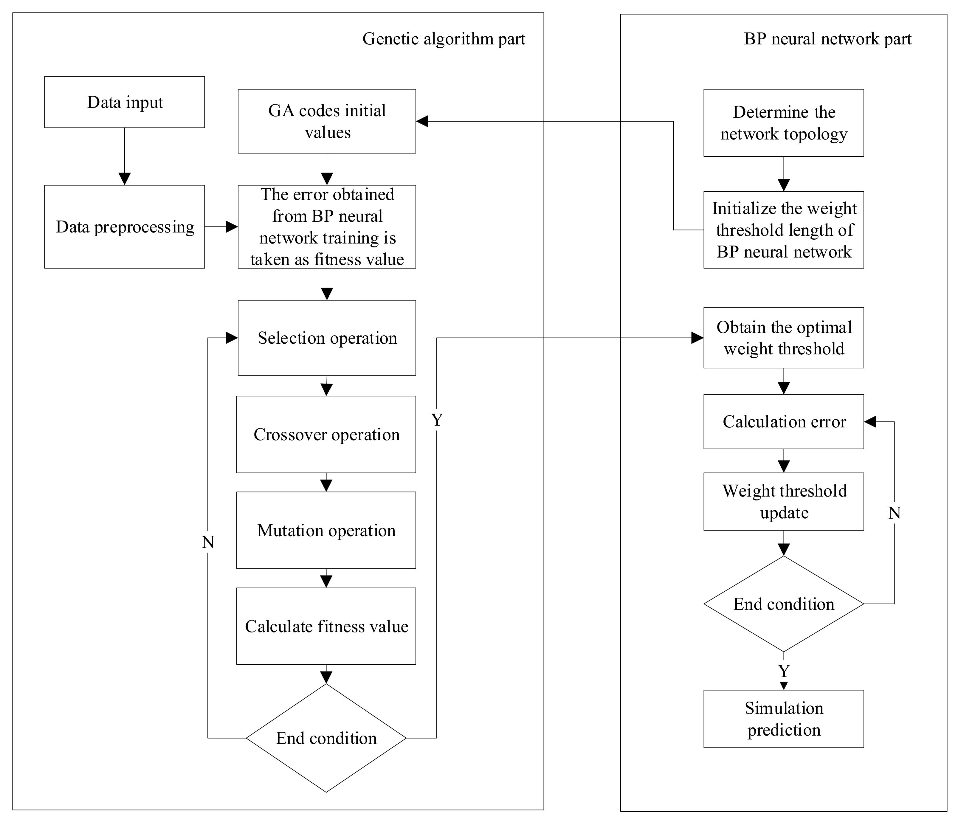
The implementation steps of the neural network prediction model based on genetic algorithm are mainly divided into two modules, the genetic algorithm part and the BP neural network part. The specific process is shown in Figure 1, and the specific implementation steps are as follows.
Step 1: Using the binary coding method, the initial weights and the threshold values of hidden layer and output layer of neural network are coded. Because the optimal number of cells in the hidden layer of neural network can be obtained experimentally, the code includes the weights and thresholds of the network and the binary serial code of the number of cells in the hidden layer of neural network.
Step 2: After the encoding mode and the composition of the binary code are determined, the system randomly generates the initial population, and the initial population number can use the best population obtained from the experiment.
Step 3: According to the definition of fitness function, first calculate the fitness value according to Equation (3). Judge whether the fitness value meets the end condition of genetic algorithm. If so, go to Step 5; if not satisfied, continue the steps in order.
Step 4: Carry out a round of selection operation and cross-mutation operation according to the rules of roulette. The probability of each round is calculated according to the cross-mutation formula. Go back to Step 3.
Step 5: At this time, the optimal initial weights of the BP neural network are obtained, and the forward propagation learning mechanism and error back propagation mechanism of BP neural network are started. The cash flow dataset is divided into three parts: a training set, a verification set, and a test set. The training set and the verification set are used to update the weights and thresholds of the cells in the network until the end condition of updating is met.
Step 6: The best model for prediction is obtained at this time. The test set is used to calculate the prediction error of the model and evaluate the prediction ability of the model.
Step 7: Choose the adaptive function and the adaptive crossover mutation formula, and repeat the above steps. The experimental prediction errors are compared, and the performance of the adaptive genetic algorithm neural network model is observed.
3. Experiments
3.1. Experimental Setup
Supervised machine learning models generally divide the data into three sets when training learning data: a training set, a verification set, and a test set.
Training set: As the data of initial training and learning of the model, the training set needs to set specific initial parameters to establish the model and train the model.
Verification set: Use the model trained by training set to predict the verification set, select the best model weight parameters, adjust the weight parameters and threshold parameters of genetic algorithm neural network, and get the best model.
Test suite: The test suite does not participate in the establishment and selection of models. After validating the optimal model, the test set is used to evaluate the performance of the model and test the generalization ability of the model.
The choice of experimental data has a great influence on the prediction accuracy of the whole prediction model, so the cash flow of a high-tech listed company from 1 January 2019 to 30 June 2019 is used as the test data.
We used the historical cash flow data of the previous 5/10/15/20/25 days as the input of the neural network for training and learning. The previous 5/10/15/20/25 groups of cash flow data were selected as the input, and the current cash flow data were used as the expected value of the model output, so as to build a neural network model based on genetic algorithm. After the training, we input the historical cash flow data of the previous 5/10/15/20/25 days, and compared the simulated cash flow data of the 6/11/16/21/26 days with the real data.
The fitness function selected the objective function of the Matlab package and improved fitness function, and the iteration time was set to 150. The selection operation used roulette, and the crossover probability and mutation probability were as shown in Table 1.
The BP neural network in this paper used the method of momentum gradient descent as the training network. The training function was the Traindm function in Matlab. The activation function, learning rate, training target error, and training times were as shown in Table 2. The input layer of the neural network was 5 neurons, the output layer was 1 neuron, and the hidden layer was 15 neurons. The initial weights and thresholds were the system defaults.
3.2. Experimental Results
In this subsection, we perform three groups of experiments, which are evaluations of optimal neuron number and optimal population, relative error evaluations, and comparative evaluations.
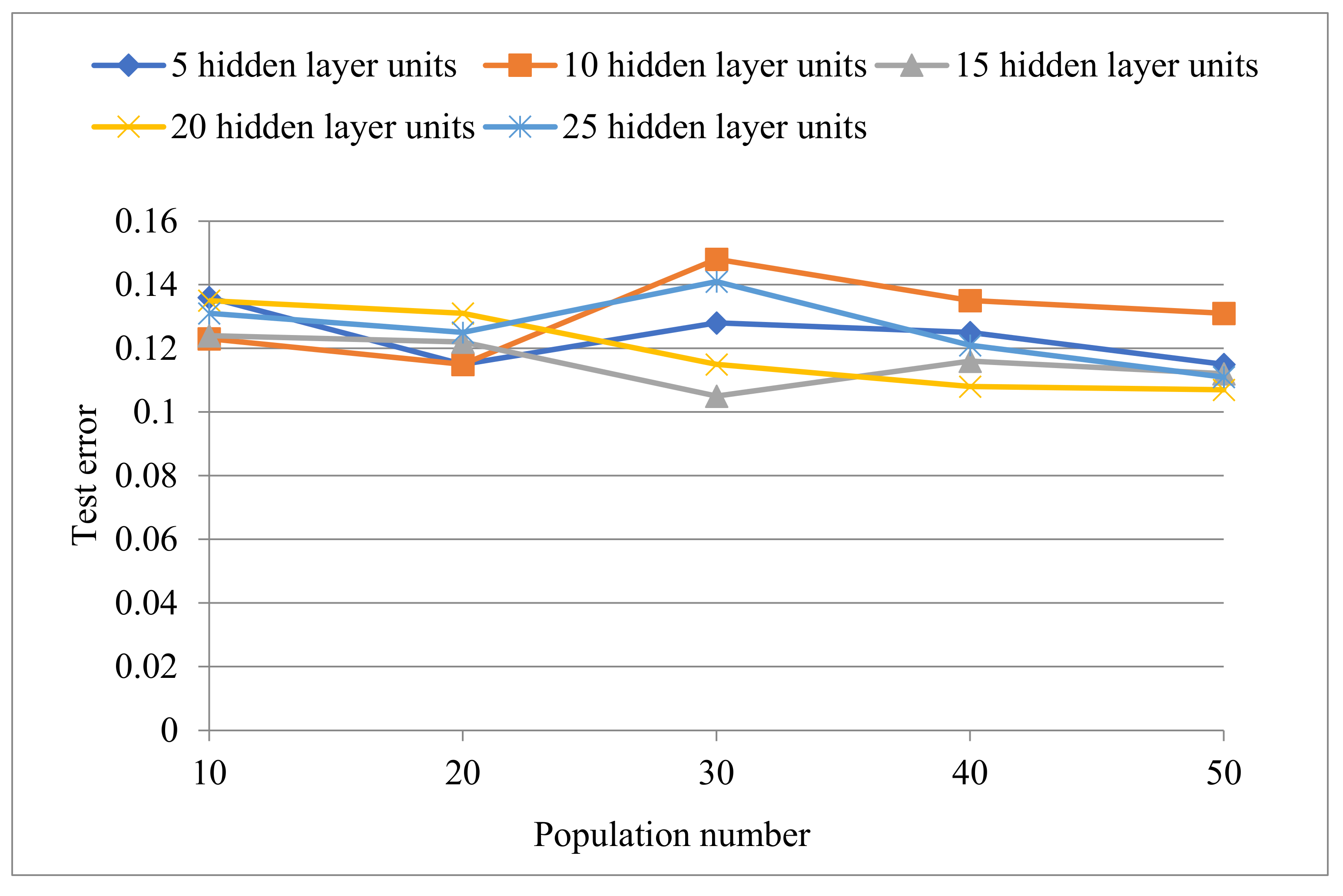
In the first groups of experiments, we performed evaluations of optimal neuron number and optimal population. For the neural network model based on the improved genetic algorithm, it is necessary to determine some fixed parameters to forecast the cash flow data. For the genetic algorithm, we needed to determine the initial population, and for the neural network, we needed to determine the number of hidden layer units. In order to study the influence of the number of neurons and the n chromosome population in the hidden layer of neural network with the best cash flow data on the model optimization results, the number of neurons in the hidden layer of neural network and the number of chromosome population, respectively, were as shown in Table 3 to predict the historical data of cash flow.
As shown in Figure 2, the historical cash flow data of the previous 5/10/15/20/25 days were selected as the training test data, and the figure shows the error diagram of the test results. In the neural network model based on the genetic algorithm, the number of hidden layer units and population of the neural network were changed, and the difference between the actual output and the expected output of the test set was observed. The difference between each combination is not large, which shows that the genetic algorithm has a strong global optimization ability and good performance.
As a result, for the historical cash flow data of the previous 5/10/15/20/25 days, when the population is 30 and the number of hidden neurons is 15, the error of the model is the smallest and the prediction ability of the model is the best.
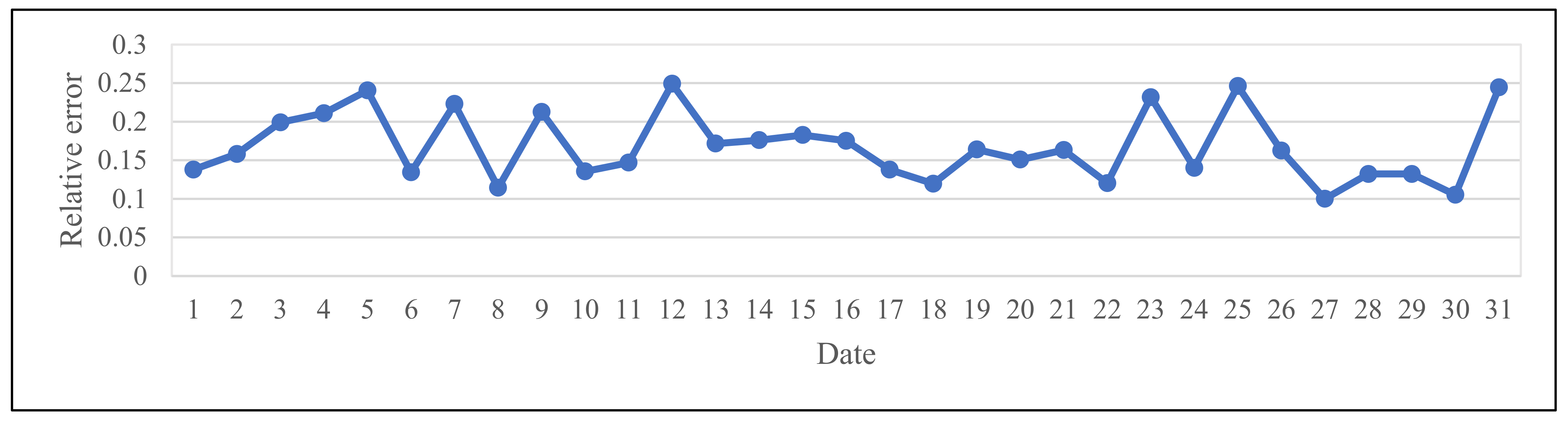
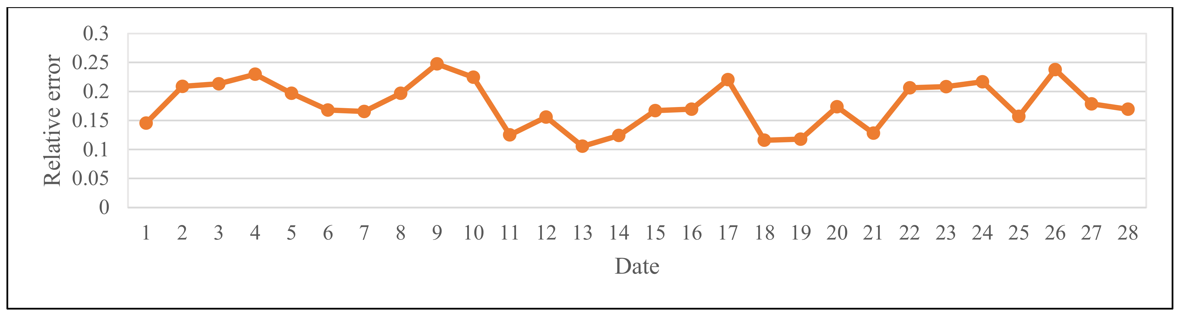
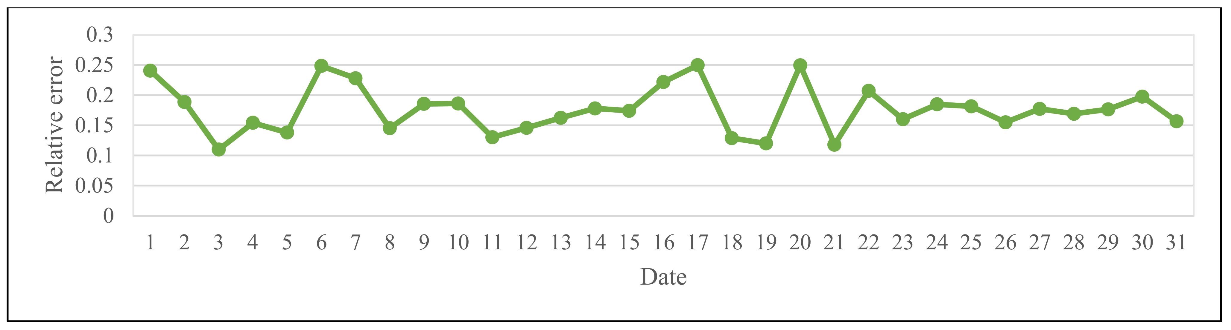
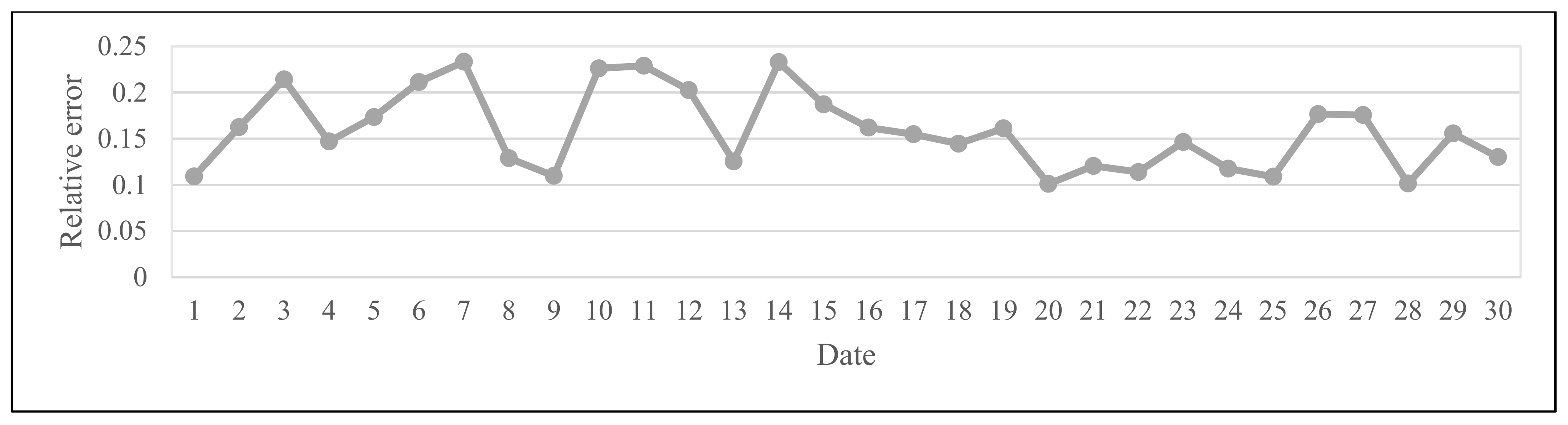
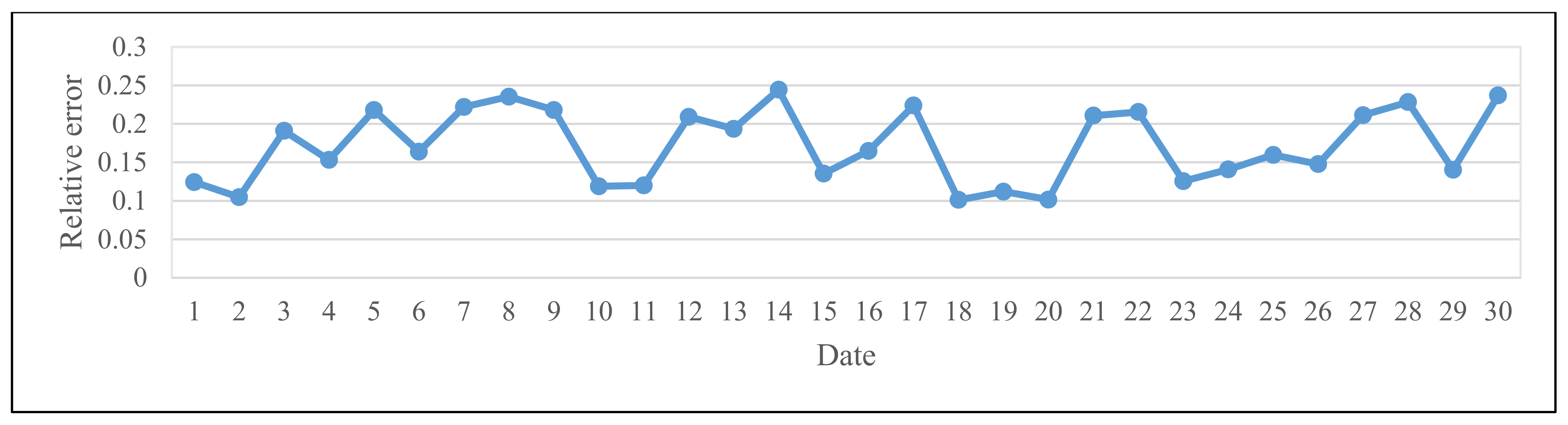
In the second group of experiments, we performed relative error evaluations. Taking the free cash flow data of G Company from 1 January 2019 to 30 June 2019 as the test data, the relative error was evaluated by using the proposed prediction model, as shown in Table 4 and Figure 3, Figure 4, Figure 5, Figure 6, Figure 7 and Figure 8. Among them, relative error refers to the ratio of the absolute value of the difference between the predicted value and the actual value of the day to the actual value of the day.
As obtained from Figure 3, Figure 4, Figure 5, Figure 6, Figure 7 and Figure 8, the minimum value of relative error data is 0.1002, the maximum value is 0.2495, and the average value is 0.1697. From the experimental results, the relative error is small, the predicted value is close to the real value, and the prediction model proposed in this paper can better predict the free cash flow of enterprises.
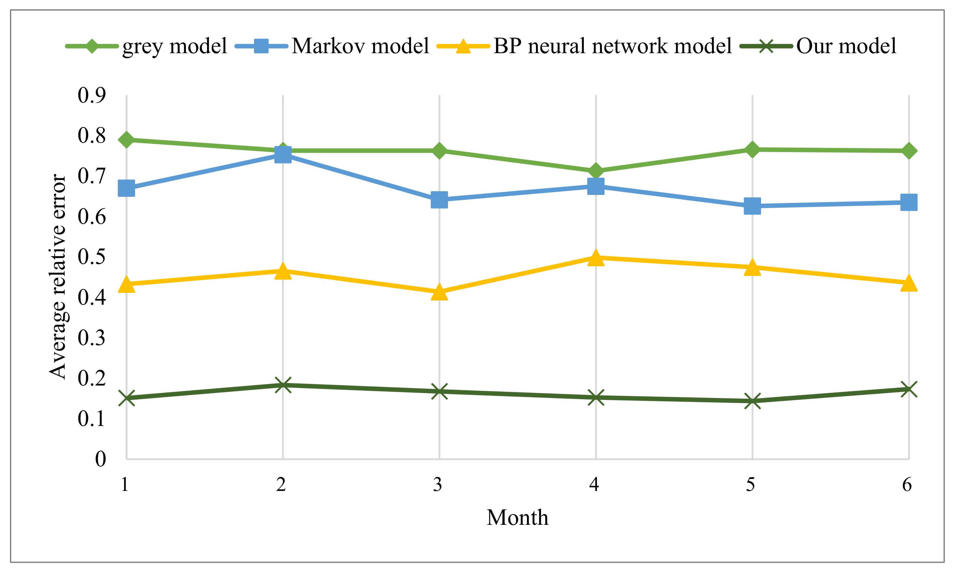
In the third groups of experiments, we performed comparative evaluations. This group of experiments will compare the relevant free cash flow prediction models, and evaluate the average relative error of free cash flow data of G Company from 1 January 2019 to 30 June 2019. It can be seen from Figure 9 that the average relative error of the forecasting model proposed in this paper is smaller than that of other free cash flow forecasting models from January 2019 to June 2019, so the forecasting model proposed in this paper has a better forecasting ability.
4. Conclusions
In this paper, a BP neural network model based on the improved genetic algorithm is proposed to predict the free cash flow of enterprises. Taking the data of G Company as an example, the optimal number of neurons and population and the relative error are evaluated by data preprocessing, the genetic algorithm, and neural network parameter selection. The experimental results show that when the population is 30 and the number of hidden layer neurons is 15, the error of the model is the smallest and the prediction ability of the model is the best. By calculating the relative error, we found that the model has high precision in forecasting free cash flow. Comparing the average relative error of relevant forecasting models shows that the forecasting model proposed in this paper has a better forecasting ability and effect.
The prediction model proposed in this paper provides a new idea for companies to predict free cash flow. On the one hand, it can predict the value of free cash flow more scientifically and objectively, which has better guiding significance for enterprise evaluation. On the other hand, it can provide a reference for company stakeholders of to carry out enterprise value management and investment management.
Author Contributions
Conceptualization, L.Z. and L.B.; Methodology, L.Z., M.Y. and L.B.; Validation, L.Z. and M.Y.; Investigation: L.Z., M.Y. and L.B.; Writing—original draft, L.Z., M.Y. and L.B.; Writing—review and editing, L.Z. and L.B.; Supervision, L.B.; Project administration, L.B. All authors have read and agreed to the published version of the manuscript.
Funding
This work was supported by the National Natural Science Foundation of China (61402087), the Natural Science Foundation of Hebei Province (F2019501030), the Natural Science Foundation of Liaoning Province (2019-MS-130), the Key Project of Scientific Research Funds in Colleges and Universities of Hebei Education Department (ZD2020402), the Fundamental Research Funds for the Central Universities (N2023019), and (in part by) the Program for 333 Talents in Hebei Province (A202001066).
Acknowledgments
The authors would also like to express their gratitude to the anonymous reviewers for providing very helpful suggestions.
Conflicts of Interest
The authors declare no conflict of interest.
References
- Fomina, O.; Moshkovska, O.; Luchyk, S.; Manachynska, Y.; Kuzub, M. Managing the Agricultural Enterprises’ Valuation: Actuarial Approach. Probl. Perspect. Manag. 2020, 18, 289–301. [Google Scholar] [CrossRef] [Green Version]
- Miciula, I.; Kadlubek, M.; Stępień, P. Modern Methods of Business Valuation—Case Study and New Concepts. Sustainability 2020, 12, 2699. [Google Scholar] [CrossRef] [Green Version]
- Huang, W.; Liu, J.; Bai, H.; Zhang, P. Value Assessment of Companies by Using an Enterprise Value Assessment System Based on Their Public Transfer Specification. Inf. Processing Manag. 2020, 57, 102254. [Google Scholar] [CrossRef]
- Gráf, P.; Rowland, Z. Potential of the Small Enterprise Value Assessment Using the Discounted FCFF Method. In Economic Systems in the New Era: Stable Systems in an Unstable World; Ashmarina, S.I., Horák, J., Vrbka, J., Šuleř, P., Eds.; IES 2020 Lecture Notes in Networks and Systems; Springer: Cham, Switzerland, 2021; Volume 160, pp. 846–855. [Google Scholar] [CrossRef]
- Liu, Y.C.; Yeh, I.C. Building Valuation Model of Enterprise Values for Construction Enterprise with Quantile Neural Networks. J. Constr. Eng. Manag. 2016, 142, 04015075. [Google Scholar] [CrossRef]
- Vochozka, M.; Rowland, Z.; Suler, P.; Marousek, J. The Influence of the International Price of Oil on the Value of the EUR/USD Exchange Rate. J. Compet. 2020, 12, 167–190. [Google Scholar] [CrossRef]
- Vochozka, M.; Horák, J.; Krulický, T.; Pardal, P. Predicting Future Brent Oil Price on Global Markets. Acta Montan. Slovaca 2020, 25, 375–392. [Google Scholar] [CrossRef]
- Luca, P.D. Enterprise Valuation. In Analytical Corporate Valuation; Springer: Cham, Switzerland, 2018; pp. 367–397. [Google Scholar] [CrossRef]
- Nekhili, M.; Amar, I.F.B.; Chtioui, T.; Lakhal, F. Free Cash Flow and Earnings Management: The Moderating Role of Governance and Ownership. J. Appl. Bus. Res. 2016, 32, 255–268. [Google Scholar] [CrossRef]
- Dewi, I.A.M.C.; Sari, M.M.R.; Budiasih, I.G.A.N.; Suprasto, H.B. Free Cash Flow Effect towards Firm Value. Int. Res. J. Manag. IT Soc. Sci. 2019, 6, 108–116. [Google Scholar] [CrossRef]
- Abdoh, H.A.A.; Varela, O. Product Market Competition, Cash Flow and Corporate Investments. Manag. Financ. 2018, 44, 207–221. [Google Scholar] [CrossRef]
- Buus, T. A General Free Cash Flow Theory of Capital Structure. J. Bus. Econ. Manag. 2015, 16, 675–695. [Google Scholar] [CrossRef] [Green Version]
- Agustia, D. Pengaruh Faktor Good Corporate Governance, Free Cash Flow, dan Leverage Terhadap Manajemen Laba. J. Akunt. Dan Keuang. 2013, 15, 27–42. [Google Scholar] [CrossRef] [Green Version]
- Park, K.; Jang, S.C. Capital Structure, Free Cash Flow, Diversification and Firm Performance: A Holistic Analysis. Int. J. Hosp. Manag. 2013, 33, 51–63. [Google Scholar] [CrossRef]
- Bukit, R.B.; Nasution, F.N. Employee Diff, Free Cash Flow, Corporate Governance and Earnings Management. Procedia Soc. Behav. Sci. 2015, 211, 585–594. [Google Scholar] [CrossRef] [Green Version]
- Chen, X.; Sun, Y.; Xu, X. Free Cash Flow, Over-Investment and Corporate Governance in China. Pac. Basin Financ. J. 2016, 37, 81–103. [Google Scholar] [CrossRef]
- Kadioglu, E.; Kilic, S.; Yilmaz, E.A. Testing the Relationship between Free Cash Flow and Company Performance in Borsa Istanbul. Int. Bus. Res. 2017, 10, 148–158. [Google Scholar] [CrossRef] [Green Version]
- Guizani, M.; Abdalkrim, G. Board Gender Diversity, Financial Decisions and Free Cash Flow: Empirical Evidence from Malaysia. Manag. Res. Rev. 2022, 45, 198–216. [Google Scholar] [CrossRef]
- Nobakht, M.; Hassanzadeh, R.B. Impact of Free Cash Flow on Real and Artificial Earnings Management. Account. Audit. Rev. 2017, 24, 421–440. [Google Scholar] [CrossRef]
- Vochozka, M.; Vrbka, J.; Suler, P. Bankruptcy or Success? The Effective Prediction of a Company’s Financial Development Using LSTM. Sustainability 2020, 12, 7529. [Google Scholar] [CrossRef]
- Luo, N.; Chen, J.; Kong, L.; Zhu, Y. Enterprise Valuation Analysis Based on Grey Prediction Model and Index Selection—A Case Study of Huayi Brothers Media Group. Int. J. Econ. Financ. 2016, 8, 11–22. [Google Scholar] [CrossRef] [Green Version]
- Yao, H.; Li, X.; Hao, Z.; Li, Y. Dynamic Asset–Liability Management in A Markov Market with Stochastic Cash Flows. Quant. Financ. 2016, 16, 1575–1597. [Google Scholar] [CrossRef]
- Rowland, Z.; Lazaroiu, G.; Podhorská, I. Use of Neural Networks to Accommodate Seasonal Fluctuations When Equalizing Time Series for the CZK/RMB Exchange Rate. Risks 2021, 9, 1. [Google Scholar] [CrossRef]
- Li, J.; Hu, H.; Li, X.; Jin, Q.; Huang, T. Economic Benefit of Shale Gas Exploitation Based on Back Propagation Neural Network. J. Intell. Fuzzy Syst. 2020, 39, 8823–8830. [Google Scholar] [CrossRef]
- Jennergren, L.P. Continuing Value in Firm Valuation by The Discounted Cash Flow Model. Eur. J. Oper. Res. 2008, 185, 1548–1563. [Google Scholar] [CrossRef]
- Décamps, J.P.; Mariotti, T.; Rochet, J.C.; Villeneuve, S. Free Cash Flow, Issuance Costs, and Stock Prices. J. Financ. 2011, 66, 1501–1544. [Google Scholar] [CrossRef]
- Tabei, S.M.A.; Bagherpour, M.; Mahmoudi, A. Application of Fuzzy Modelling to Predict Construction Projects Cash Flow. Period. Polytech. Civ. Eng. 2019, 63, 647–659. [Google Scholar] [CrossRef]
- Weytjens, H.; Lohmann, E.; Kleinsteuber, M. Cash Flow Prediction: MLP and LSTM Compared to ARIMA and Prophet. Electron. Commer. Res. 2021, 21, 371–391. [Google Scholar] [CrossRef]
- Hsu, S.C. Fuzzy Time Series Customers Prediction: Case Study of an E-Commerce Cash Flow Service Provider. Int. J. Comput. Intell. Appl. 2016, 15, 1650024. [Google Scholar] [CrossRef]
- Wang, J.S.; Ning, C.X. ANFIS Based Time Series Prediction Method of Bank Cash Flow Optimized by Adaptive Population Activity PSO Algorithm. Information 2015, 6, 300–313. [Google Scholar] [CrossRef] [Green Version]
Figure 1.
Neural network prediction flowchart based on the improved genetic algorithm.

Figure 2.
Test error of different populations.

Figure 3.
Relative error of cash flow forecast of G company in January 2019.

Figure 4.
Relative error of cash flow forecast of G company in February 2019.

Figure 5.
Relative error of cash flow forecast of G company in March 2019.

Figure 6.
Relative error of cash flow forecast of G company in April 2019.

Figure 7.
Relative error of cash flow forecast of G company in May 2019.

Figure 8.
Relative error of cash flow forecast of G company in June 2019.

Figure 9.
Average relative errors of different prediction models.


Table 1.
Parameters of genetic algorithm.
| Initial Parameters of Genetic Algorithm | Value |
|---|---|
| Population size | 30 |
| Number of iterations | 150 |
| Crossing probability | 0.9 |
| Crossing probability | 0.1 |
| Select operation | Roulette |
| Fitness function | Matlab’s own function |
Table 2.
Parameters of neural network.
| Initial Parameters of Neural Network | Value |
|---|---|
| Number of input layers | 5 |
| Number of hidden layers | 15 |
| Number of output layers | 1 |
| Target error | 1 × 10⁻⁶ |
| Training times | 10,000 |
| Learning rate | 0.01 |
| Training function | Traindm function |
| Training method | Momentum gradient descent |
| Activation function | Sigmoid function |
| Network weights and thresholds | Optimal weights obtained by genetic algorithm |
Table 3.
The errors of selecting different parameters.
| Number of Hidden Layer Units | Population | Test Error |
|---|---|---|
| 5 | 10 | 0.136 |
| 5 | 20 | 0.115 |
| 5 | 30 | 0.128 |
| 5 | 40 | 0.125 |
| 5 | 50 | 0.115 |
| 10 | 10 | 0.123 |
| 10 | 20 | 0.115 |
| 10 | 30 | 0.148 |
| 10 | 40 | 0.135 |
| 10 | 50 | 0.131 |
| 15 | 10 | 0.124 |
| 15 | 20 | 0.122 |
| 15 | 30 | 0.105 |
| 15 | 40 | 0.116 |
| 15 | 50 | 0.112 |
| 20 | 10 | 0.135 |
| 20 | 20 | 0.131 |
| 20 | 30 | 0.115 |
| 20 | 40 | 0.108 |
| 20 | 50 | 0.107 |
| 25 | 10 | 0.131 |
| 25 | 20 | 0.125 |
| 25 | 30 | 0.141 |
| 25 | 40 | 0.121 |
| 25 | 50 | 0.111 |
Table 4.
Relative errors (RE) of cash flow forecast of G company from 1 January 2019 to 30 June 2019.
Table 4.
Relative errors (RE) of cash flow forecast of G company from 1 January 2019 to 30 June 2019.
| Date | January 1 | January 2 | January 3 | January 4 | January 5 | January 6 | January 7 | January 8 | January 9 |
| RE | 0.1379 | 0.1582 | 0.1992 | 0.2110 | 0.2405 | 0.1343 | 0.2230 | 0.1143 | 0.2127 |
| Date | January 10 | January 11 | January 12 | January 13 | January 14 | January 15 | January 16 | January 17 | January 18 |
| RE | 0.1356 | 0.1470 | 0.2492 | 0.1716 | 0.1761 | 0.1828 | 0.1752 | 0.1378 | 0.1197 |
| Date | January 19 | January 20 | January 21 | January 22 | January 23 | January 24 | January 25 | January 26 | January 27 |
| RE | 0.1640 | 0.1509 | 0.1633 | 0.1204 | 0.2318 | 0.1401 | 0.2462 | 0.1625 | 0.1002 |
| Date | January 28 | January 29 | January 30 | January 31 | February 1 | February 2 | February 3 | February 4 | February 5 |
| RE | 0.1323 | 0.1323 | 0.1052 | 0.2446 | 0.1454 | 0.2088 | 0.2132 | 0.2296 | 0.1967 |
| Date | February 6 | February 7 | February 8 | February 9 | February 10 | February 11 | February 12 | February 13 | February 14 |
| RE | 0.1679 | 0.1655 | 0.1967 | 0.2476 | 0.2245 | 0.1251 | 0.1558 | 0.1056 | 0.1241 |
| Date | February 15 | February 16 | February 17 | February 18 | February 19 | February 20 | February 21 | February 22 | February 23 |
| RE | 0.1669 | 0.1694 | 0.2203 | 0.1159 | 0.1177 | 0.1735 | 0.1280 | 0.2063 | 0.2082 |
| Date | February 24 | February 25 | February 26 | February 27 | February 28 | March 1 | March 2 | March 3 | March 4 |
| RE | 0.2167 | 0.1570 | 0.2375 | 0.1786 | 0.1693 | 0.2404 | 0.1885 | 0.1098 | 0.1540 |
| Date | March 5 | March 6 | March 7 | March 8 | March 9 | March 10 | March 11 | March 12 | March 13 |
| RE | 0.1379 | 0.2483 | 0.2279 | 0.1451 | 0.1854 | 0.1861 | 0.1302 | 0.1458 | 0.1623 |
| Date | March 14 | March 15 | March 16 | March 17 | March 18 | March 19 | March 20 | March 21 | March 22 |
| RE | 0.1779 | 0.1740 | 0.2217 | 0.2495 | 0.1287 | 0.1199 | 0.2494 | 0.1178 | 0.2070 |
| Date | March 23 | March 24 | March 25 | March 26 | March 27 | March 28 | March 29 | March 30 | March 31 |
| RE | 0.1601 | 0.1847 | 0.1814 | 0.1549 | 0.1772 | 0.1690 | 0.1764 | 0.1974 | 0.1565 |
| Date | April 1 | April 2 | April 3 | April 4 | April 5 | April 6 | April 7 | April 8 | April 9 |
| RE | 0.1091 | 0.1625 | 0.2142 | 0.1470 | 0.1734 | 0.2114 | 0.2333 | 0.1289 | 0.1097 |
| Date | April 10 | April 11 | April 12 | April 13 | April 14 | April 15 | April 16 | April 17 | April 18 |
| RE | 0.2262 | 0.2290 | 0.2027 | 0.1254 | 0.2329 | 0.1872 | 0.1620 | 0.1548 | 0.1446 |
| Date | April 19 | April 20 | April 21 | April 22 | April 23 | April 24 | April 25 | April 26 | April 27 |
| RE | 0.1612 | 0.1011 | 0.1205 | 0.1139 | 0.1464 | 0.1176 | 0.1088 | 0.1767 | 0.1756 |
| Date | April 28 | April 29 | April 30 | May 1 | May 2 | May 3 | May 4 | May 5 | May 6 |
| RE | 0.1014 | 0.1556 | 0.1301 | 0.1778 | 0.2072 | 0.2248 | 0.1470 | 0.1235 | 0.1862 |
| Date | May 7 | May 8 | May 9 | May 10 | May 11 | May 12 | May 13 | May 14 | May 15 |
| RE | 0.1692 | 0.2379 | 0.2152 | 0.1855 | 0.1012 | 0.2121 | 0.1032 | 0.1896 | 0.1529 |
| Date | May 16 | May 17 | May 18 | May 19 | May 20 | May 21 | May 22 | May 23 | May 24 |
| RE | 0.1371 | 0.2294 | 0.1563 | 0.1272 | 0.1616 | 0.1369 | 0.1943 | 0.1391 | 0.2316 |
| Date | May 25 | May 26 | May 27 | May 28 | May 29 | May 30 | May 31 | June 1 | June 2 |
| RE | 0.1248 | 0.1354 | 0.1238 | 0.2109 | 0.1152 | 0.1405 | 0.1278 | 0.1243 | 0.1047 |
| Date | June 3 | June 4 | June 5 | June 6 | June 7 | June 8 | June 9 | June 10 | June 11 |
| RE | 0.1910 | 0.1531 | 0.2179 | 0.1639 | 0.2220 | 0.2353 | 0.2180 | 0.1189 | 0.1200 |
| Date | June 12 | June 13 | June 14 | June 15 | June 16 | June 17 | June 18 | June 19 | June 20 |
| RE | 0.2091 | 0.1935 | 0.2445 | 0.1353 | 0.1649 | 0.2239 | 0.1012 | 0.1120 | 0.1016 |
| Date | June 21 | June 22 | June 23 | June 24 | June 25 | June 26 | June 27 | June 28 | June 29 |
| RE | 0.2108 | 0.2154 | 0.1255 | 0.1407 | 0.1597 | 0.1477 | 0.2113 | 0.2283 | 0.1403 |
| Date | June 30 | ||||||||
| RE | 0.2369 |
Publisher’s Note: MDPI stays neutral with regard to jurisdictional claims in published maps and institutional affiliations. |
© 2022 by the authors. Licensee MDPI, Basel, Switzerland. This article is an open access article distributed under the terms and conditions of the Creative Commons Attribution (CC BY) license (https://creativecommons.org/licenses/by/4.0/).
Share and Cite
MDPI and ACS Style
Zhu, L.; Yan, M.; Bai, L. Prediction of Enterprise Free Cash Flow Based on a Backpropagation Neural Network Model of the Improved Genetic Algorithm. Information 2022, 13, 172. https://doi.org/10.3390/info13040172
AMA Style
Zhu L, Yan M, Bai L. Prediction of Enterprise Free Cash Flow Based on a Backpropagation Neural Network Model of the Improved Genetic Algorithm. Information. 2022; 13(4):172. https://doi.org/10.3390/info13040172
Chicago/Turabian StyleZhu, Lin, Mingzhu Yan, and Luyi Bai. 2022. "Prediction of Enterprise Free Cash Flow Based on a Backpropagation Neural Network Model of the Improved Genetic Algorithm" Information 13, no. 4: 172. https://doi.org/10.3390/info13040172
Note that from the first issue of 2016, this journal uses article numbers instead of page numbers. See further details here.