
Selected Methods of Predicting Financial Health of Companies: Neural Networks Versus Discriminant Analysis


Department of Finance, Accounting and Mathematical Methods, Faculty of Management and Business, University of Prešov, Konštantínova 16, 080 01 Prešov, Slovakia
*
Author to whom correspondence should be addressed.
Information 2021, 12(12), 505; https://doi.org/10.3390/info12120505
Submission received: 24 October 2021
/
Revised: 25 November 2021
/
Accepted: 2 December 2021
/
Published: 6 December 2021
(This article belongs to the Special Issue Evaluating Methods and Decision Making)
Abstract
:This paper focuses on the financial health prediction of businesses. The issue of predicting the financial health of companies is very important in terms of their sustainability. The aim of this paper is to determine the financial health of the analyzed sample of companies and to distinguish financially healthy companies from companies which are not financially healthy. The analyzed sample, in the field of heat supply in Slovakia, consisted of 444 companies. To fulfil the aim, appropriate financial indicators were used. These indicators were selected using related empirical studies, a univariate logit model and a correlation matrix. In the paper, two main models were applied—multivariate discriminant analysis (MDA) and feed-forward neural network (NN). The classification accuracy of the constructed models was compared using the confusion matrix, error type 1 and error type 2. The performance of the models was compared applying Brier score and Somers’ D. The main conclusion of the paper is that the NN is a suitable alternative in assessing financial health. We confirmed that high indebtedness is a predictor of financial distress. The benefit and originality of the paper is the construction of an early warning model for the Slovak heating industry. From our point of view, the heating industry works in the similar way in other countries, especially in transition economies; therefore, the model is applicable in these countries as well.
1. Introduction
It is the interest of every business owner to evaluate the financial health of their company as quickly and as easily as possible. From this point of view, it is important to find out, in particular, whether the company is able to increase its value and thus provide a guarantee that the investment in the company will receive a return. The question remains how to measure and predict the financial health of a company. The most important measure is the monitoring of the financial performance of the company. There are a number of approaches to measure a company’s financial health and predict its financial distress and bankruptcy, but their use depends on the current market situation, as there is a shift in the development of these measures applied for financial health prediction [1].
When choosing the method of measuring the financial health of the company, we took into account the study by Coats and Fant [2], who focused on the creation of a NN in order to predict the future financial health of companies. They created a framework of financial indicators that can distinguish healthy companies from companies which are in financial distress. At the same time, these authors pointed to the restrictive assumptions of the MDA, which do not have to be met when using a NN. It is also possible to follow the study of Anandarajan et al. [3], who created the distress prediction model using an ANN. Other authors who applied NNs in predicting financial distress are Etheridge and Sriram [4], Abid and Zouari [5].
In accordance with the abovementioned research studies, we have set the following aim of the paper: to determine the financial health of the analyzed sample of companies and to distinguish financially healthy companies from companies which are not financially healthy; and to identify financial indicators that are predictors of financial distress. The purpose is to detect early warning signals for unfavorable financial conditions in currently viable companies. To fulfill this goal, we applied both the MDA model and the NN model and compared the classification ability of these models. The vast majority of authors apply these methods in the field of corporate bankruptcy prediction. In our research, we applied them to predict financial distress. For this study, we selected the heating industry, because we have been dealing with the assessment of financial health of businesses from this industry for a longer period of time.
The heating industry is crucial for every economy. It is a specific sector, which is important from both an economic and social point of view and plays an important role in daily lives of society and consumers. Companies operating in the Slovak heating industry are local central heat supply systems. Some of them have a monopoly position in a given geographical area. Another specific feature of this industry is that heat cannot be traded between countries and, due to significant heat losses in transmission and distribution, it cannot be traded between networks existing in individual locations [6]. Due to the mentioned specifics, it is not appropriate to predict the financial health of companies operating in the Slovak heating industry by applying commonly used models. In the paper we fill this gap and propose a model for the heating industry, which can be applied not only for Slovak businesses but also for businesses operating under similar conditions, for example in transition economies. In this model, we applied indicators, which are slightly different from other studies. Our aim was to contribute to the confirmation of the importance of NNs in predicting financial distress on a sample of Slovak companies.
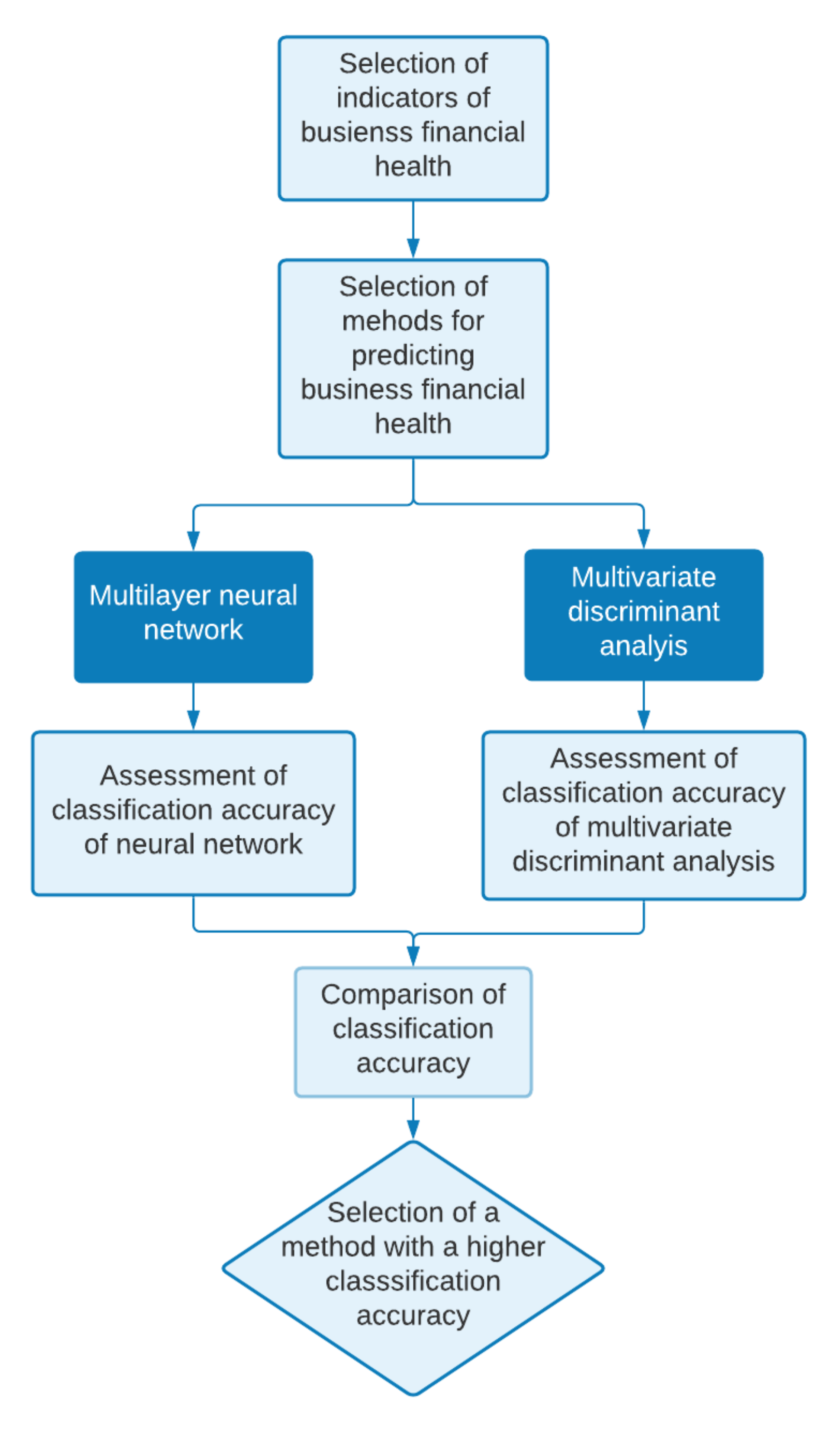
The remainder of the paper is structured as follows. Section 1 outlines the most important research and studies in which NNs have been applied in predicting corporate financial health. Section 2 is divided: into Section 2.1.: Definitions of financial distress as a prerequisite for bankruptcy; and Section 2.2.: Review of the studies dealing with financial distress and bankruptcy applying MDA and NN. Section 3 describes the analyzed sample of companies and characterizes in more detail the methods applied in predicting the financial health as well as the possible financial failure of companies. The Results section lists the results of the analyzed models and the results of their ability to predict financial distress. The Discussion section presents conclusions and findings, which includes a confirmation of the high classification ability of our NN. This section contains also limitations and future research. The process of the research is illustrated in Figure 1.
2. Literature Review
A financially healthy company is a company that meets two basic conditions: namely liquidity, i.e., it is able to repay its liabilities on time; and at the same time is profitable, i.e., it achieves a return on the capital invested in the business. If the company does not meet these two conditions, it is in financial distress. In general, the term financial distress usually brings about negative connotations as it describes the financial health of a company—especially a lack of liquidity and inability to repay liabilities [7].
2.1. Definitions of Financial Distress as a Prerequisite for Bankruptcy
In this part of the study, we focused on defining the financial distress of companies, which may be a prerequisite for their bankruptcy. It is necessary to point out that financial distress is not the same as bankruptcy, but it can be a sign of it. Such a situation does not have to end in bankruptcy if the necessary measures are implemented.
Although in this study we deal with financial distress, we wish to define the concept of business bankruptcy. We agree with opinion of Klieštik et al. [7] who considers bankruptcy a formal termination of the company’s existence due to the valid legislation of the respective country.
According to Dimitras et al. [8], bankruptcy can be defined as a situation where a company is unable to repay liabilities to its creditors, pay preference shares to shareholders, pay its suppliers or has overdrawn its accounts or the company has gone bankrupt under the relevant law. The authors Ding et al. [9] state that bankruptcy is a situation where the company is unable to pay its liabilities, priority dividends and has overdrawn its accounts. In the vast majority of sources dealing with the issue, the authors define bankruptcy as the inability of the company to repay its liabilities, thus triggers bankruptcy processes [10]. Financial distress is one of the most important indications of bankruptcy; therefore we deal with it in the following text.
Altman and Hotchkiss [11] defined the concept of financial distress and pointed out that bankruptcy represents the legal end of financial distress. Hendel [12] uses the probabilistic approach and defines financial distress as the probability of bankruptcy, which depends on the level of liquid assets as well as the availability of credit.
Platt and Platt’s [13] (p. 155) hypothesis is that “financial distress is something that happens to companies as a consequence of operating decisions or external forces while bankruptcy is something that companies choose to do to protect their assets from creditors”.
Financial distress is different from bankruptcy; it occurs when the firm may not be able to meet its financial obligations because of a decrease in the firm’s business operations, illiquid assets and high fixed costs. By contrast, bankruptcy is a final state in which firms stop doing business because of that financial distress. In some cases, financial distress can be detected before the company falls into insolvency. Therefore, financial distress does not always progress to bankruptcy [14].
The following Table 1 sets out the different views on the definition of financial distress as a negative state of financial health of companies, which can be an indication of their possible bankruptcy.
2.2. Rerview of the Studies Dealing with Financial Distress and Bankruptcy Applying MDA and NN
In the recent past, more than 30 different methods have emerged that predominantly use programming and artificial intelligence to predict the financial situation of companies. Messier and Hansen [30] In [31] were among the first to apply an expert system in bankruptcy prediction.
The first experiments with artificial models that mimicked the biological nervous system date back to the 1920s. However, it took another 20 years to lay the foundations for a scientific discipline dealing with artificial neural networks. The first theoretical work dealing with the issue is the work of McCulloch and Pitts [32]. In this work, they pointed out the possibility of the existence of an artificial neural network that could work with arithmetic or logical formulas. This work influenced other scientists who began to deal with neural networks from a practical point of view [33]. At the turn of the 1940s and 1950s, the laws of learning a neural network with layered feedforward topology were described [34] In [33]. In the 1950s and 1960s, the first experiments with a simple single-layer neural network for a real numerical range of parameters took place. This network was created by a single neuron, and this simple type of network was called the “perceptron” [35]. It was the simplest neural network constructed in 1958 by Rosenblatt. This model consisted of several company inputs and one output. These experiments were terminated because it was found that the linear neural network algorithm was not suitable for solving tasks that are more complex. This limitation could be removed by constructing a multilayer network [33]. The turning point in the development came at the turn of the 1970s and 1980s, when an algorithm for the backpropagation of errors for the training of multilayer neural networks was discovered [33]. Although backpropagation is not a general algorithm for learning neural networks, it can solve a large number of problems that single-layer perceptrons cannot solve. It should be noted that the backpropagation algorithm is currently the most widely used neural network method [36].
The neural network method has several variations. The most common is the multilayer perceptron (MLP). The multilayer perceptron is an important component of artificial neural networks (ANNs), developed to mimic the ability of humans to learn and generalize, which sought to model the functions of biological neural networks [37]. Multilayer feedforward neural networks (MLPs) trained by the backpropagation algorithm provide a non-statistical and nonlinear approach to bankruptcy prediction. MLP-based models are more reliable in predicting bankruptcy than logistic regression and multiple discriminant analysis (MDA) [38,39,40]. However, MLPs are affected by a number of constraints (e.g., local minima and over-adaptation) and their predictive power depends on a number of parameters (e.g., typology, learning) [41].
Other versions of neural networks are, for example, the CASCOR network, probabilistic neural networks, self-organizing maps (the main representative of a self-organizing neural network with learning without a teacher is the Kohonen network or Kohonen map, which was introduced by Kohonen in 1982 [42]), learning vectors (Support Vector Machine—SVM) and many more. A study by Odom and Sharda [43], which was mentioned in the introduction, developed a neural network model to predict bankruptcy. The model uses financial data from various companies. The same set of data was also analyzed using a more traditional method of predicting bankruptcy, namely multivariate discriminant analysis. The results of both methods were be compared and the higher predictive power of the neural network was confirmed. The study by Huang and Zhang [44] describes the use of artificial neural networks in the field of production. According to these authors, a self—organizing map (SOM) is very often used in predicting bankruptcy. It is a suitable tool for predicting possible bankruptcy. The authors used this map to analyze and visualize the financial situation of companies over several years through a two-step clustering process [45].
A study by Wilson and Sharda [38] confirms the estimation accuracy of neural networks and classical multidimensional discriminant analysis in predicting business bankruptcy. The estimation accuracy of these two techniques is presented in a comprehensive, statistically reliable framework that indicates the value added to the problem of forecasting the bankruptcy using each technique. The study suggests that neural networks perform significantly better than discriminant analysis in predicting corporate bankruptcies.
Lee and Choi [46] also confirmed the predictive ability of neural networks. According to these authors, accurate prediction of business bankruptcy is a challenging issue. This paper presents a multi-industry investigation into the bankruptcy of Korean companies using back-propagation neural network. Sectors that were analyzed include construction, retail and manufacturing. The aim of the study was to propose a specific model for predicting bankruptcy in selected industries, which was based on the selection of appropriate independent variables. In the study, the estimation accuracy of a back-propagation neural network was compared with the accuracy of multidimensional discriminant analysis. The results show that the prediction using the selected industries sample exceeds the prediction using the whole sample, by 6–12%. The estimation accuracy of bankruptcy prediction using the back-propagation neural network is greater than the accuracy of multiple discriminant analysis. The study proposes knowledge about a practical industry model of bankruptcy prediction.
Raghupathi et al. [47] discuss the application of the error back-propagation network in making bankruptcy prediction decisions. In their study, they present the results of simulations with one and two hidden layers with different nodes. The configuration with two hidden layers was be found to have excellent classification accuracy compared to the single hidden layer configuration. Based on their initial results, it seems that neural network algorithms can been further explored as potential models for predicting bankruptcy.
Shah et al. [48] have also confirmed the importance of neural networks in the field of bankruptcy prediction. According to them, the neural network-based model works as well, if not better, than some existing studies (In 1968, Altman developed a model of multidimensional discriminant analysis (MDA), known as the Z-score. Since Altman’s study [49], the number as well as the complexity of these models have increased dramatically. It was used, among others, by Blum [50]; Deakin [51]; Elam [52]; Norton and Smith [53]; Wilcox [54]; Taffler [55]. Logistic regression was firstly used by Martin [56] to predict bankruptcy of banks and by Ohlson [57] to predict bankruptcy of companies. Simak [58] was the first who thought of using the DEA method.) However, it must be acknowledged that these results are limited by the software solution and the choice of financial ratios.
Hongkyu et al. [59] also point out the prediction of bankruptcy as a significant problem in the classification of companies. In their study, they applied three different techniques: multidimensional discriminant analysis, case-based forecasting and a neural network. They used these methods to predict bankrupt and non-bankrupt Korean companies. The average hit ratios of these three methods ranged from 81.5% to 83.8%. However, the neural network worked better than the other two methods.
The Gherghina study [60] was very useful. His empirical study looked at an approach based on the application of artificial intelligence (AI) to detect bankruptcy in companies. He pointed out that AI is mostly employed in expert systems (ES). He also pointed out the application of the EC prototype to assess the risk of company failure and used indebtedness and solvency indicators to do so.
Other authors who made use of neural networks in their works on bankruptcy prediction include Atiya [40], Altman et al. [61], Abid and Zouari [62], Du Jardin [63], Zouari [64] and Vochozka and Rowland [65].
In 2010, Du Jardin [63] investigated the prediction accuracy of various prediction models. He found out that the neural network, which is based on a set of selected financial indicators, achieves better predictive results compared to other models.
3. Data and Methodology
The MDA forecasts the financial situation of a company using various characteristics, i.e., using a certain set of indicators, which are usually assigned different weights. In the discriminant analysis models, various financial indicators and variables are applied, which form one aggregate number—the multidimensional discriminant scores. The main benefit of this method is the inclusion of companies in groups based on discriminant scores. Most studies that deal with this method are based on the assumption that a low value of the discriminant score signals poor financial health of the company [66].
If all independent variables are taken into account when creating a discriminant function, can use canonical discriminant analysis. Its most important task is to find a way to differentiate between prosperous and non-prosperous enterprises, as well as to minimize intra-group variability and maximize inter-group variability. In order to best distinguish the two groups of enterprises, a model of multidimensional discriminant analysis is constructed which consists of a linear combination of variables and aims at identifying among those enterprises that are likely to fail and those that are unlikely to fail.
For the enterprise i, the discriminant function is expressed by the formula (1):
where
—value of variable xj for the enterprise i,
—coefficients of canonical variable for j = 1, ..... , p,
—constant.
The constant “w” is calculated according to the relation (2):
where
—is the average of all determined values of the quantity, for j = 1, ... , p.
To divide enterprises into prosperous and non-prosperous, a vector of average values of discriminants in groups of enterprises, i.e., centroids for prosperous and non-prosperous enterprises () should be calculated. The formula (3) is as follows:
The impact of individual explanatory variables can be expressed using the standardized canonical discriminant function coefficients as well as the correlations coefficients between discriminating variables and the standardized canonical discriminant function. Standardized coefficients are used to determine which explanatory variables have the best discriminatory ability.
The quality of the discriminant model can be assessed using the statistical significance of the discriminant function. If the created canonical discriminant function distinguishes between prosperous and non-prosperous enterprises, the model is statistically significant. The distinction between these groups of enterprises is because the differences in the mean values of the variables that are included in the model are statistically significant. The statistical significance of each discriminator is tested by analysis of variance. Wilk’s Lambda can be applied as a test statistic [67].
The classification ability of the discriminant model is assessed based on the confusion matrix. This matrix contains the absolute and relative numbers of enterprises classified into individual groups correctly and incorrectly. To confirm the classification ability of the model, the samples are divided into training (80%) and testing (20%). If the sample is not large enough, it is not divided, but cross validation is used instead. The most commonly used method is the one-leave-out classification, which is implemented by dividing a set of enterprises into K equal or approximately equal parts. The model is considered suitable if a 25% higher classification accuracy is achieved than in the case of random classification of enterprises into individual groups. In the case of two groups of enterprises, namely prosperous and non-prosperous enterprises, the model could be considered suitable if its classification accuracy is at least 75% of correctly classified enterprises [7].
However, the use of multidimensional discriminant analysis requires that the following assumptions are met [66]:
- quantitative or binary characters;
- none of the characters may be a linear combination of another character or characters;
- it is not appropriate to use two or more strongly correlated characters at the same time;
- the covariance matrices for each group must be approximately identical;
- the characteristics describing each group should meet the requirement of a multidimensional normal distribution.
At the same time, it is preferable that the number of discriminatory variables is lower than the number of subjects in the analyzed sample [68]. The condition of normal distribution of variables over time has not been observed for a long time, because it is very difficult to comply with this condition in terms of financial indicators. In addition, based on the research results of Klieštik et al. [7], a part of the companies is always incorrectly classified and penetrations occur because the homogeneity of the failing companies is not guaranteed due to the different causes of their financial problems. However, the aim is to keep the number of misclassified companies as low as possible.
The non-parametric NN method does not require the fulfillment of the prerequisites required by the MDA, in particular the normal distribution and conformity of covariance matrices. This is why we used this method.
At present, the development of new types of ANN continues. However, implementation of ANNs is limited. In practice, MLP is the most widespread network because perceptrons could solve only linearly separable problems. However, most real problems are non-linear. Rumelhat et al. [69] introduced the error backpropagation method for feed-forward ANN with hidden layers in 1986. This multilayer feed-forward neural network, which follows this rule, is also able to solve nonlinear problems.
The feed-forward neural network is a feed-forward connection (i is a neuron of m-layer and j is a neuron of (m-1)-layer) between neurons, with each neuron of one layer transmitting signals to each neuron of the next layer. A neuron works with two types of inputs, namely, inputs from other neurons and inputs from the environment. Input from the external environment is a threshold value—bias (θ). The outputs of each neurons are while i is a number of neurons (i = 1, 2 … n) in m-layer. The total number of layers is M, while the input layer is marked 0. The activation values of a neuron are marked as , where (m = 1, 2 … M). The activation values of the input neurons are . The total outputs of the network are , where and M is the last layer of the network. NN methodology processed according to authors [70,71]. The general formula for calculating the activation value of any neuron and any layer is calculated according to the relation (4):
where
—represents the total input to the i-neuron of m-layer, which is calculated as the sum of the product of the weight going from j-neuron to i-neuron and the activation value of the neuron from which the signal originates
N—is the number of neurons in the input layer,
θ—is the value of the neuron threshold,
F—is an activating function, usually a unipolar sigmoidal function is used—, or other functions (hyperbolic tangent, function with fixed boundary signum).
If the signal is propagated up to the output layer, an error signal can be calculated. This signal should be calculated differently for the output and differently for the hidden layers. For the output layer, the error signal (δ) is calculated as follows (5):
where,
—total output of the i-neuron of M-layer,
—derivation of the activation function in
—required output of the i-neuron,
—difference between expected and obtained network output.
When propagating an error through other layers, it is possible to calculate the error signal according to the formula (6):
where
—is the multiple of the weight coming from the j-neuron to i-neuron of m-layer and the error of the neuron of the layer into which the signal enters.
After propagating the error across the network, the weights are modified so that the size of the error is as small as possible. This modification takes place according to the relationship (7):
where
—is a new, modified scale,
—is the old value of the scale,
—is the weight gain,
—error signal of j-neuron on m-layer,
η—network learning speed.
Subsequently, it is necessary to assess whether the network also complies with the data outside the training set. If the error for the training set is comparable to the error for the testing set, the model is acceptable. If the model is not valid then it is necessary to:
- test other initial values for the instrument;
- modify the MLP scheme (change the number of vertices, layers);
- try another ANN method;
- reject ANN as a suitable method.
The empirical study deals with the issue of MLP with two hidden layers. MLP was applied to the data of heat management companies in Slovakia. In total, there are around 590 companies operating in the selected sector, employing approximately 17,430 employees. The share of the sector in the sales of Slovak industry is on average around 12.4% and the average value of production is at the level of 10.64 billion EUR. In 2021, a significant increase in production and sales was recorded in the given sector, namely by 1.64% compared to 2020. This increase in share is the most significant increase since 2013.
A sample used in this empirical study consisted of 458 heat supply companies. From this sample, we excluded 14 companies, which achieved extreme values and degenerated mean values. Therefore, we performed the analysis on a sample of 444 companies. Of the total number of registered enterprises of the given branch of business in Slovakia, the sample of 444 companies represented 75%. The financial statements of companies for 2016, for which the forecast of financial failure of companies was made, were provided by the Slovak analytical agency CRIF—Slovak Credit Bureau, s.r.o. [70]. Companies were divided into prosperous and non-prosperous based on the indicator indebtedness. The number of prosperous companies was 366, the number of non-prosperous was 78.
The sample of the companies was divided into a training and testing group. The training group consisted of 298 companies, which represents 67% of the validation group of companies, and the test group was formed of 146 companies (33%). The selection of indicators for forecasting the financial failure of companies is in Table 2. We started the analysis with 19 indicators from all areas of financial health assessment and, using a correlation matrix and a one-dimensional logit model, we reduced this number to 11 indicators. Correlation matrix is stated in Appendix A (Table A1). Based on its results, we can say that there is strong statistically significant relationship between the indicators TL, CL and QR, indicators CPP, CTC and ROS and indicators EFAR and ELFAR. From these groups of indicators we used only one indicator. In order to eliminate multicollinearity, we did not use indicator TDTA, which was applied as a financial distress criterion.
4. Results
At the beginning of the analysis and prediction of the financial health of enterprises and their possible bankruptcy, means, medians and standard deviations were calculated for selected financial indicators, especially for the group of enterprises that were prosperous and non-prosperous (Table 3).
Based on the results of a Mann–Whitney U test (Table 4) for these two groups of enterprises, it could be stated that enterprises that face financial distress show deficiencies in the values of indicators CL, ACP, TATR, ICR, EDR. EFAR, CR. The values of these indicators show that these enterprises should focus on improving these areas of assessing their financial health so that they are not at risk of bankruptcy.
4.1. Results of Discriminant Analysis
When creating the discriminant function all independent variables were taken into account. To test the normality of financial ratios, we used Shapiro–Wilk test. The results show that financial ratios do not have the properties of normal distribution (see Appendix B and Appendix C, Table A2 and Table A3).
In order to find whether covariance matrices were equal, we used Box’s M test, Based on its results (Table 5) we state that the covariance matrices cannot be considered equal.
Despite the fact that financial ratios do not have the properties of normal distribution and covariance matrices are not equal, we constructed a discriminant analysis model. When using financial indicators, it is difficult to meet the conditions required by discriminant analysis.
From the results of the discriminant analysis (Table 6), it is clear that the following indicators had the highest impact on discriminatory scores: equity to debt ratio—positive impact; cost ratio—negative impact; and equity to fixed assets ratio—positive impact. Other significant discriminators in the order include: return on costs; total assets turnover ratio; and average collection period. Based on the above, it can be stated that these indicators are significant discriminators in the classification of enterprises as facing bankruptcy and not facing bankruptcy.
The influence of the explanatory variables on the discriminatory ability of the model was also confirmed by the correlation coefficients calculation (the discriminant function and the individual explanatory variables).
The calculation confirmed the influence of the above indicators on the value of the discriminant score.
The created discriminant function-D, which is used to calculate the discriminant score, has the following form:
Results were confirmed by the stepwise model; after the exclusion of each indicator, the results were approximately the same. The statistical significance of mean differences was tested by analysis of variance using Wilks’ Lambda. The results are shown in Table 7. Since the vectors of the mean values of the variables included in this function were statistically significant, canonical discriminant function well separates between the groups of prosperous enterprises and non-prosperous enterprises. It was also noticed that 84% of variance in discriminant scores was not explained by group differences.
Centroids were calculated using the model. The centroids showed how individual groups of enterprises differed from each other given the canonical variable. Centroid for enterprises belonging to the group of prosperous enterprises reached the value of 0.203. On the other hand, the centroid for non-prosperous enterprises reached the value of −0.951.
The classification ability of the created model was assessed using a Confusion matrix (Table 8). The overall classification ability of the model is 84%. Classification ability for prosperous businesses is 98.9%, for non-prosperous businesses it is 15.4%. Model for original sample achieved Error type 1 at the level of 84.6% and error type 2 at the level of 1.1%. Due to the fact that the sample was not large enough to be divided into training and testing, cross validation was performed with 83.33% of cross-validated grouped cases correctly classified.
Based on the results of the confusion matrix we can conclude that the MDA model achieved a very good overall classification ability and excellent classification ability for prosperous businesses. On the other hand, its classification ability for non-prosperous businesses was low. Results achieved in this study can be compared with the results of other studies. Khemais et al. [71] achieved 76.3% classification ability for healthy businesses and 76.5% classification ability for failing businesses. Mihalovič: [72], in his study, achieved 45.61% classification ability for bankrupt businesses and 81.97% classification ability for non-bankrupt businesses.
4.2. Results of Neural Networks
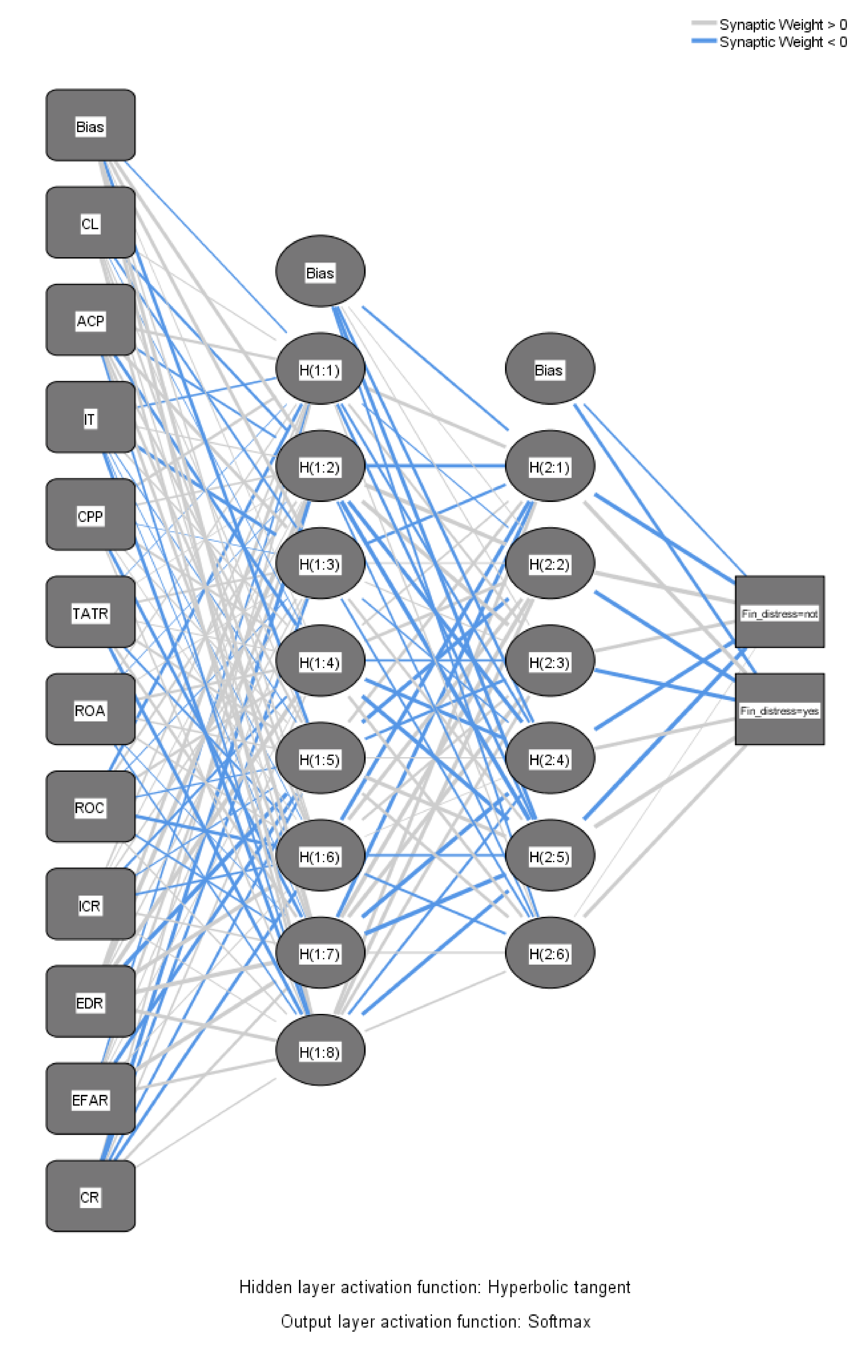
We applied a four-layer MLP. which consisted of one input layer, two hidden layers and one output layer. The model worked with 11 financial indicators at the input layer. These represented all areas of the enterprise’s financial health. The list of indicators and the method of their calculation is given in the Table 1. To these input indicators was added the unit bias, which acted as a constant in the regression analysis (b). The first hidden layer was formed by 8 units and unit b and the second hidden layer by 6 units and unit b. The output layer represents one dependent variable—bankruptcy—while the total number of units was equal to 2. The network parameters can be seen in the Table 9.
Figure 2 shows the MLP, which was constructed to predict a group of enterprises facing bankruptcy and those which are not.
The resulting values of the model significance are given in the Table 10 for the training sample and the testing sample. Since the given values are approximately the same, it can be stated that the model is acceptable and has a good predictive power.
The results in the Table 11 show that both the training and testing samples achieved excellent results in classification accuracy when predicting corporate bankruptcy. Overall classification ability of the model for the training sample was 98.3%; classification ability for prosperous businesses was 99.2%, for non-prosperous 93.8%. The model for the training sample achieved error type 1 at the level of 6.2% and error type 2 at the level of 0.8%. Results of the model for the testing sample were similar, with overall classification ability being 95.9%; classification ability for prosperous businesses was 98.3%, for non-prosperous 86.7%. The model for the testing sample achieved error type 1 at the level of 13.3% and error type 2 at the level of 1.7%. Based on the results of confusion matrix we can conclude that the NN model achieved very good results for prosperous as well as non-prosperous businesses.
Quality of constructed models was evaluated with the use of Brier score and Somers’ D, also called Gini coefficient (Table 12). Brier score takes values from 0 to 1. The ideal case is 0. Somers’ D takes values from −1 to 1. Ideal case is 1. We can conclude that MLP achieved excellent results, while MDA achieved worse results.
5. Discussion
The study confirmed that the neural network is an important and precise tool for predicting corporate bankruptcy. The classification accuracy of the neural network, for prosperous and non-prosperous businesses, is high. The network, however, has a disadvantage: it is not possible to use it to determine significant discriminators for predicting corporate bankruptcy. The method should be supplemented with the results of the method, which provides this information.
The classification ability of MDA was excellent in the case of prosperous businesses, but for non-prosperous businesses it was low. This might have been caused by the fact that conditions of normal distribution and equality of covariance matrices were violated in this study. When using financial indicators as independent variables, it is very difficult to meet them. Therefore, it was necessary to supplement MDA with NN.
The initial analysis of the financial condition of enterprises showed that companies facing bankruptcy show problems in the indicators of solvency, capital structure, stability and costs, namely CL, ACP, TATR, ICR, EDR. EFAR, CR. These indicators were determined by the Mann–Whitney U test. The discriminant analysis confirmed that of these indicators, the most significant discriminators for confirming the bankruptcy are CR, EFAR, and EDR, followed by the indicators TATR, ROC and ACP. This confirmed the assumption according to the Mann–Whitney test regarding the significance of the difference between the above indicators with regard to enterprises facing and not facing bankruptcy was correct. The biggest financial problem of this sample of enterprises active in the heat management sector is the high indebtedness (up to 84%). It can be stated that the indebtedness of the enterprise is a significant predictor of bankruptcy, as indicators EDR and EFAR achieved the highest coefficient in MDA.
Research needs to be continued and developed further. The aim is to focus on an even more detailed and refined selection of inputs to the neural network. For this purpose, genetic algorithms [73] and the LASSO method [74] could be used in the future. These methods allow for the selection of indicators, which proved to be important predictors of bankruptcy. The sample of companies studied in the future research should be larger in order to make acceptable generalizations in the field. Since our research focuses on the application of the DEA method in predicting the bankruptcy of enterprises, it would be beneficial to compare the results of DEA models with the results of neural networks in future research. It is already clear that the DEA has its advantages compared to the neural network in setting the target values of input and output variables.
The limiting factors of this research were a smaller sample of companies and extreme values of indicators. However, research in bankruptcy prediction of an analyzed sample of businesses is becoming more and more relevant. Recently, there has been a significant increase in energy prices in Slovakia, which has had a negative impact on the financial health of companies.
In the case of discriminant analysis, the problem is regarding the normal distribution, because it is very difficult to meet this condition for financial indicators. It must therefore be borne in mind that, in this case, some enterprises were misclassified. Despite this fact, the results of DA were presented.
Each of the applied methods has its strengths as well as weaknesses. In practice, however, several methods should be used and their results should be compared. There is specialized software for all prediction methods. However, the personal contribution of managers and their experience and knowledge in the field, as well as in the selection of input indicators, is very important.
Author Contributions
J.H., M.M. and I.P. contributed to all aspects of this work. All authors have read and agreed to the published version of the manuscript.
Funding
This research received no external funding.
Institutional Review Board Statement
Not applicable.
Informed Consent Statement
Not applicable.
Data Availability Statement
Financial statements in the form of balance sheets and profit and loss statements were obtained from the agency CRIF—Slovak Credit Bureau, s.r.o., which deals with the collection and processing of financial statements of Slovak companies according to individual SK NACE. Information was provided by a third party, which is focused on data collection and cooperation with academic institutions and supports them in obtaining the necessary data for their research activities. These financial statements have been prepared by the company by mutual agreement and according to the requirements of the author.
Acknowledgments
This paper was prepared within the grant scheme VEGA No. 1/0741/20 (the application of variant methods in detecting symptoms of possible bankruptcy of Slovak businesses in order to ensure their sustainable development).
Conflicts of Interest
The authors declare no conflict of interest.
Appendix A

Table A1.
Correlation matrix.
| Variable | Marked Correlations Are Significant at p < 0.05000 | ||||||||||||||||||
|---|---|---|---|---|---|---|---|---|---|---|---|---|---|---|---|---|---|---|---|
| TL | CL | QR | ACP | IT | CPP | CTC | TATR | ROA | ROE | ROS | ROC | TDTA | ER | ICR | EDR | EFAR | ELFAR | CR | |
| TL | 1.0000 | 0.9998 | 0.9187 | 0.0058 | −0.0046 | −0.0099 | 0.0128 | −0.0795 | 0.0125 | −0.0108 | 0.0126 | 0.0249 | −0.0142 | 0.0142 | −0.0122 | 0.0374 | 0.0061 | 0.0073 | −0.0144 |
| p = −−− | p = 0.00 | p = 0.00 | p = 0.901 | p = 0.921 | p = 0.832 | p = 0.785 | p = 0.089 | p = 0.790 | p = 0.817 | p = 0.787 | p = 0.595 | p = 0.762 | p = 0.762 | p = 0.794 | p = 0.424 | p = 0.896 | p = 0.877 | p = 0.758 | |
| CL | 0.9998 | 1.0000 | 0.9163 | 0.0057 | −0.0055 | −0.0100 | 0.0128 | −0.0798 | 0.0125 | −0.0107 | 0.0126 | 0.0265 | −0.0139 | 0.0139 | −0.0119 | 0.0379 | 0.0065 | 0.0077 | −0.0142 |
| p = 0.00 | p = −−− | p = 0.00 | p = 0.903 | p = 0.906 | p = 0.831 | p = 0.784 | p = 0.088 | p = 0.789 | p = 0.819 | p = 0.787 | p = 0.572 | p = 0.766 | p = 0.766 | p = 0.799 | p = 0.418 | p = 0.890 | p = 0.870 | p = 0.762 | |
| QR | 0.9187 | 0.9163 | 1.0000 | 0.0056 | −0.0054 | −0.0084 | 0.0110 | −0.0858 | 0.0082 | −0.0095 | 0.0108 | 0.0220 | −0.0120 | 0.0120 | −0.0145 | 0.0426 | 0.0119 | 0.0132 | −0.0127 |
| p = 0.00 | p = 0.00 | p = −−− | p = 0.906 | p = 0.907 | p = 0.857 | p = 0.814 | p = 0.066 | p = 0.861 | p = 0.840 | p = 0.817 | p = 0.639 | p = 0.798 | p = 0.798 | p = 0.757 | p = 0.363 | p = 0.799 | p = 0.777 | p = 0.786 | |
| ACP | 0.0058 | 0.0057 | 0.0056 | 1.0000 | 0.0186 | 0.5913 | −0.4051 | 0.0051 | 0.0015 | −0.0003 | −0.3983 | −0.0159 | 0.0009 | −0.0010 | 0.0014 | 0.0076 | 0.0013 | 0.0012 | 0.0010 |
| p = 0.901 | p = 0.903 | p = 0.906 | p = −−− | p = 0.691 | p = 0.00 | p = 0.00 | p = 0.913 | p = 0.974 | p = 0.995 | p = 0.000 | p = 0.735 | p = 0.985 | p = 0.982 | p = 0.976 | p = 0.872 | p = 0.978 | p = 0.980 | p = 0.983 | |
| IT | −0.0046 | −0.0055 | −0.0054 | 0.0186 | 1.0000 | 0.0564 | −0.0578 | 0.0437 | 0.0001 | −0.0167 | −0.0166 | −0.0218 | −0.0037 | 0.0036 | −0.0043 | −0.0161 | −0.0038 | −0.0043 | −0.0036 |
| p = 0.921 | p = 0.906 | p = 0.907 | p = 0.691 | p = −−− | p = 0.228 | p = 0.217 | p = 0.350 | p = 0.998 | p = 0.721 | p = 0.722 | p = 0.641 | p = 0.937 | p = 0.938 | p = 0.927 | p = 0.731 | p = 0.935 | p = 0.926 | p = 0.939 | |
| CPP | −0.0099 | −0.0100 | −0.0084 | 0.5913 | 0.0564 | 1.0000 | −0.9769 | −0.0154 | −0.0012 | 0.0031 | −0.9740 | −0.0304 | −0.0017 | 0.0017 | −0.0020 | −0.0006 | −0.0018 | −0.0021 | −0.0016 |
| p = 0.832 | p = 0.831 | p = 0.857 | p = 0.00 | p = 0.228 | p = −−− | p = 0.00 | p = 0.742 | p = 0.979 | p = 0.947 | p = 0.00 | p = 0.517 | p = 0.971 | p = 0.972 | p = 0.967 | p = 0.991 | p = 0.969 | p = 0.965 | p = 0.973 | |
| CTC | 0.0128 | 0.0128 | 0.0110 | −0.4051 | −0.0578 | −0.9769 | 1.0000 | 0.0189 | 0.0018 | −0.0036 | 0.9987 | 0.0302 | 0.0022 | −0.0022 | 0.0026 | 0.0026 | 0.0024 | 0.0026 | 0.0021 |
| p = 0.785 | p = 0.784 | p = 0.814 | p = 0.00 | p = 0.217 | p = 0.00 | p = −−− | p = 0.686 | p = 0.969 | p = 0.938 | p = 0.00 | p = 0.519 | p = 0.963 | p = 0.963 | p = 0.956 | p = 0.955 | p = 0.959 | p = 0.955 | p = 0.965 | |
| TATR | −0.0795 | −0.0798 | −0.0858 | 0.0051 | 0.0437 | −0.0154 | 0.0189 | 1.0000 | 0.0124 | 0.0254 | 0.0221 | 0.0244 | −0.0239 | 0.0239 | 0.0486 | −0.0075 | −0.0031 | −0.0053 | −0.0273 |
| p = 0.089 | p = 0.088 | p = 0.066 | p = 0.913 | p = 0.350 | p = 0.742 | p = 0.686 | p = −−− | p = 0.792 | p = 0.588 | p = 0.637 | p = 0.602 | p = 0.610 | p = 0.610 | p = 0.298 | p = 0.873 | p = 0.947 | p = 0.909 | p = 0.559 | |
| ROA | 0.0125 | 0.0125 | 0.0082 | 0.0015 | 0.0001 | −0.0012 | 0.0018 | 0.0124 | 1.0000 | 0.0601 | 0.0026 | 0.1063 | −0.0084 | 0.0085 | 0.0089 | 0.0226 | 0.0153 | 0.0156 | −0.0044 |
| p = 0.790 | p = 0.789 | p = 0.861 | p = 0.974 | p = 0.998 | p = 0.979 | p = 0.969 | p = 0.792 | p = −−− | p = 0.199 | p = 0.956 | p = 0.023 | p = 0.857 | p = 0.857 | p = 0.849 | p = 0.629 | p = 0.744 | p = 0.738 | p = 0.925 | |
| ROE | −0.0108 | −0.0107 | −0.0095 | −0.0003 | −0.0167 | 0.0031 | −0.0036 | 0.0254 | 0.0601 | 1.0000 | −0.0025 | 0.0452 | −0.0040 | 0.0040 | 0.0075 | −0.0179 | 0.0061 | 0.0079 | −0.0098 |
| p = 0.817 | p = 0.819 | p = 0.840 | p = 0.995 | p = 0.721 | p = 0.947 | p = 0.938 | p = 0.588 | p = 0.199 | p = −−− | p = 0.957 | p = 0.333 | p = 0.932 | p = 0.932 | p = 0.873 | p = 0.702 | p = 0.896 | p = 0.867 | p = 0.835 | |
| ROS | 0.0126 | 0.0126 | 0.0108 | −0.3983 | −0.0166 | −0.9740 | 0.9987 | 0.0221 | 0.0026 | −0.0025 | 1.0000 | 0.0303 | 0.0021 | −0.0021 | 0.0025 | 0.0023 | 0.0024 | 0.0026 | 0.0022 |
| p = 0.787 | p = 0.787 | p = 0.817 | p = 0.000 | p = 0.722 | p = 0.00 | p = 0.00 | p = 0.637 | p = 0.956 | p = 0.957 | p = −−− | p = 0.518 | p = 0.964 | p = 0.964 | p = 0.957 | p = 0.961 | p = 0.959 | p = 0.955 | p = 0.962 | |
| ROC | 0.0249 | 0.0265 | 0.0220 | −0.0159 | −0.0218 | −0.0304 | 0.0302 | 0.0244 | 0.1063 | 0.0452 | 0.0303 | 1.0000 | 0.0017 | −0.0017 | 0.0057 | 0.0201 | 0.0060 | 0.0077 | −0.0058 |
| p = 0.595 | p = 0.572 | p = 0.639 | p = 0.735 | p = 0.641 | p = 0.517 | p = 0.519 | p = 0.602 | p = 0.023 | p = 0.333 | p = 0.518 | p = −−− | p = 0.972 | p = 0.972 | p = 0.903 | p = 0.668 | p = 0.899 | p = 0.870 | p = 0.902 | |
| TDTA | −0.0142 | −0.0139 | −0.0120 | 0.0009 | −0.0037 | −0.0017 | 0.0022 | −0.0239 | −0.0084 | −0.0040 | 0.0021 | 0.0017 | 1.0000 | −1.0000 | −0.0024 | −0.0210 | −0.0028 | −0.0033 | −0.0005 |
| p = 0.762 | p = 0.766 | p = 0.798 | p = 0.985 | p = 0.937 | p = 0.971 | p = 0.963 | p = 0.610 | p = 0.857 | p = 0.932 | p = 0.964 | p = 0.972 | p = −−− | p = 0.00 | p = 0.958 | p = 0.654 | p = 0.952 | p = 0.944 | p = 0.991 | |
| ER | 0.0142 | 0.0139 | 0.0120 | −0.0010 | 0.0036 | 0.0017 | −0.0022 | 0.0239 | 0.0085 | 0.0040 | −0.0021 | −0.0017 | −1.0000 | 1.0000 | 0.0024 | 0.0210 | 0.0028 | 0.0033 | 0.0005 |
| p = 0.762 | p = 0.766 | p = 0.798 | p = 0.982 | p = 0.938 | p = 0.972 | p = 0.963 | p = 0.610 | p = 0.857 | p = 0.932 | p = 0.964 | p = 0.972 | p = 0.00 | p = −−− | p = 0.958 | p = 0.653 | p = 0.952 | p = 0.944 | p = 0.992 | |
| ICR | −0.0122 | −0.0119 | −0.0145 | 0.0014 | −0.0043 | −0.0020 | 0.0026 | 0.0486 | 0.0089 | 0.0075 | 0.0025 | 0.0057 | −0.0024 | 0.0024 | 1.0000 | 0.0036 | −0.0007 | −0.0015 | −0.0028 |
| p = 0.794 | p = 0.799 | p = 0.757 | p = 0.976 | p = 0.927 | p = 0.967 | p = 0.956 | p = 0.298 | p = 0.849 | p = 0.873 | p = 0.957 | p = 0.903 | p = 0.958 | p = 0.958 | p = −−− | p = 0.939 | p = 0.988 | p = 0.974 | p = 0.953 | |
| EDR | 0.0374 | 0.0379 | 0.0426 | 0.0076 | −0.0161 | −0.0006 | 0.0026 | −0.0075 | 0.0226 | −0.0179 | 0.0023 | 0.0201 | −0.0210 | 0.0210 | 0.0036 | 1.0000 | 0.0294 | 0.0236 | −0.0176 |
| p = 0.424 | p = 0.418 | p = 0.363 | p = 0.872 | p = 0.731 | p = 0.991 | p = 0.955 | p = 0.873 | p = 0.629 | p = 0.702 | p = 0.961 | p = 0.668 | p = 0.654 | p = 0.653 | p = 0.939 | p = −−− | p = 0.530 | p = 0.614 | p = 0.707 | |
| EFAR | 0.0061 | 0.0065 | 0.0119 | 0.0013 | −0.0038 | −0.0018 | 0.0024 | −0.0031 | 0.0153 | 0.0061 | 0.0024 | 0.0060 | −0.0028 | 0.0028 | −0.0007 | 0.0294 | 1.0000 | 0.9979 | −0.0035 |
| p = 0.896 | p = 0.890 | p = 0.799 | p = 0.978 | p = 0.935 | p = 0.969 | p = 0.959 | p = 0.947 | p = 0.744 | p = 0.896 | p = 0.959 | p = 0.899 | p = 0.952 | p = 0.952 | p = 0.988 | p = 0.530 | p = −−− | p = 0.00 | p = 0.940 | |
| ELFAR | 0.0073 | 0.0077 | 0.0132 | 0.0012 | −0.0043 | −0.0021 | 0.0026 | −0.0053 | 0.0156 | 0.0079 | 0.0026 | 0.0077 | −0.0033 | 0.0033 | −0.0015 | 0.0236 | 0.9979 | 1.0000 | −0.0039 |
| p = 0.877 | p = 0.870 | p = 0.777 | p = 0.980 | p = 0.926 | p = 0.965 | p = 0.955 | p = 0.909 | p = 0.738 | p = 0.867 | p = 0.955 | p = 0.870 | p = 0.944 | p = 0.944 | p = 0.974 | p = 0.614 | p = 0.00 | p = −−− | p = 0.934 | |
| CR | −0.0144 | −0.0142 | −0.0127 | 0.0010 | −0.0036 | −0.0016 | 0.0021 | −0.0273 | −0.0044 | −0.0098 | 0.0022 | −0.0058 | −0.0005 | 0.0005 | −0.0028 | −0.0176 | −0.0035 | −0.0039 | 1.0000 |
| p = 0.758 | p = 0.762 | p = 0.786 | p = 0.983 | p = 0.939 | p = 0.973 | p = 0.965 | p = 0.559 | p = 0.925 | p = 0.835 | p = 0.962 | p = 0.902 | p = 0.991 | p = 0.992 | p = 0.953 | p = 0.707 | p = 0.940 | p = 0.934 | p = −−− | |
Legend: TL—Total liquidity, CL—Current ratio, QR—Quick ratio, ACP—Average collection period, IT—Inventory turnover, CPP—Creditors payment period, CTC—Cash−to−cash, TATR—Total assets turnover ratio, ROA—Return on assets, ROE—Return on equity, ROS—Return on sales, ROC—Return on costs, TDTA—Total debt to total assets, ER—Equity ratio, ICR—Interest coverago ratio, EDR—Equity to debt ratio, EFAR—Equity to fixed assets ratio, ELFAR—Equity and long−term liabilities to fixed assets ratio, CR—Costs ratio.
Appendix B
Table A2.
Results of Shapiro–Wilk test—prosperous businesses.
| Variable | Obs | W | V | z | Prob > z |
|---|---|---|---|---|---|
| CL | 366 | 0.29307 | 179.757 | 12.302 | 0.00000 |
| ACP | 366 | 0.25657 | 189.037 | 12.421 | 0.00000 |
| IT | 366 | 0.19004 | 205.956 | 12.625 | 0.00000 |
| CPP | 366 | 0.25360 | 189.793 | 12.431 | 0.00000 |
| TATR | 366 | 0.55332 | 113.581 | 11.214 | 0.00000 |
| ROA | 366 | 0.35685 | 163.540 | 12.078 | 0.00000 |
| ROC | 366 | 0.39979 | 152.621 | 11.914 | 0.00000 |
| ICR | 366 | 0.11195 | 225.811 | 12.843 | 0.00000 |
| EDR | 366 | 0.24298 | 192.493 | 12.464 | 0.00000 |
| EFAR | 366 | 0.21987 | 198.371 | 12.536 | 0.00000 |
| CR | 366 | 0.22825 | 196.239 | 12.510 | 0.00000 |
Source: authors.
Appendix C
Table A3.
Results of Shapiro–Wilk test—non−prosperous businesses.
| Variable | Obs | W | V | z | Prob > z |
|---|---|---|---|---|---|
| CL | 78 | 0.28634 | 47.979 | 8.469 | 0.00000 |
| ACP | 78 | 0.54110 | 30.852 | 7.503 | 0.00000 |
| IT | 78 | 0.32882 | 45.124 | 8.335 | 0.00000 |
| CPP | 78 | 0.33201 | 44.909 | 8.324 | 0.00000 |
| TATR | 78 | 0.41853 | 39.092 | 8.021 | 0.00000 |
| ROA | 78 | 0.21245 | 52.947 | 8.685 | 0.00000 |
| ROC | 78 | 0.22597 | 52.038 | 8.647 | 0.00000 |
| ICR | 78 | 0.17952 | 55.161 | 8.774 | 0.00000 |
| EDR | 78 | 0.87917 | 8.124 | 4.583 | 0.00000 |
| EFAR | 78 | 0.30125 | 46.977 | 8.423 | 0.00000 |
| CR | 78 | 0.67947 | 21.549 | 6.718 | 0.00000 |
Source: authors.
References
- Mokrišová, M.; Horváthová, J. Bankruptcy Prediction Applying Multivariate Techniques. J. Manag. Bus. Res. Pract. 2020, 12, 52–69. Available online: http://www.journalmb.eu/archiv/JMB−2−2020.pdf#page=52 (accessed on 1 June 2021).
- Coats, P.K.; Fant, F.L. Recognizing financial distress patterns using a neural network tool. Financ. Manag. 1993, 22, 142–155. [Google Scholar] [CrossRef]
- Anandarajan, M.; Lee, P.; Anandarajan, A. Bankruptcy prediction of financially stressed firms: An examination of the predictive accuracy of artificial neural networks. Int. J. Intell. Syst. Account. Financ. Manag. 2001, 10, 69–81. [Google Scholar] [CrossRef]
- Etheridge, H.L.; Sriram, R.S. A comparison of the relative costs of financial distress models: Artificial neural networks, logit and multivariate discriminant analysis. Intell. Syst. Account. Financ. Manag. 1997, 6, 235–248. [Google Scholar] [CrossRef]
- Abid, F.; Zouari, A. Financial Distress Prediction Using Neural Networks. In Proceedings of the MS’ 2000 International Conference on Modeling and Simulation, Las Palmas de Gran Canaria, Spain, 25–27 September 2000; pp. 399–406. [Google Scholar] [CrossRef]
- Antimonopoly Office of the Slovak Republic. Functioning and Problems in the Heat Management Sector in the Slovak Republic with a Focus on Local Central Heat Supply Systems from the Perspective of the Antimonopoly Office of the Slovak Republic. 2013. Available online: http://www.antimon.gov.sk/data/att/365.pdf (accessed on 21 June 2021).
- Klieštik, T.; Válášková, K.; Klieštiková, J.; Kováčová, M.; Švábová, L. Predikcia Finančného Zdravia Podnikov Tranzitívnych Ekonomík; EDIS: Žilina, Slovakia, 2019. [Google Scholar]
- Dimitras, A.I.; Zanakis, S.H.; Zopounidis, C. A survey of business failures with an emphasis on prediction methods and industrial applications. Eur. J. Oper. Res. 1996, 90, 487–513. [Google Scholar] [CrossRef]
- Ding, Y.S.; Song, X.P.; Zen, Y.M. Forecasting Financial Condition of Chinese Listed Companies Based on Support Vector Machine. Expert Syst. Appl. 2008, 34, 3081–3089. [Google Scholar] [CrossRef]
- Pervan, I.; Pervan, M.; Vukoja, B. Prediction of company bankruptcy using statistical techniques. Croat. Oper. Res. Rev. 2011, 11, 158–166. Available online: https://hrcak.srce.hr/96660 (accessed on 11 February 2021).
- Altman, E.I.; Hotchkiss, E. Corporate Financial Distress and Bankruptcy: Predict and Avoid Bankruptcy, Analyze and Invest in Distressed Debt; John Wiley & Sons: Hoboken, NJ, USA, 2006. [Google Scholar]
- Hendel, I. Competition under financial Distress. J. Ind. Econ. 1996, 54, 309–324. [Google Scholar] [CrossRef]
- Platt, H.D.; Platt, M. Comparing Financial Distress and Bankruptcy. Rev. Appl. Econ. 2006, 2, 1–27. Available online: https://ssrn.com/abstract=876470 (accessed on 18 November 2021).
- Pham, B.; Do, T.; Vo, D. Financial distress and bankruptcy prediction: An appropriate model for listed firms in Vietnam. Econ. Syst. 2018, 42, 616–624. [Google Scholar] [CrossRef]
- Foster, G. Financial Statement Analysis, 2nd ed.; Prentice−Hall: Englewood Cliffs, NJ, USA, 1986; pp. 31–53. [Google Scholar]
- Wruck, K.H. Financial Distress, Reorganization, and Organizational Efficiency. J. Financ. Econ. 1990, 27, 419–444. [Google Scholar] [CrossRef]
- Opler, T.; Titman, S. Financial Distress and Corporate Performance. J. Financ. 1994, 49, 1015–1040. [Google Scholar] [CrossRef]
- Andrade, G.; Kaplan, S.N. How Costly is Financial (Not Economic) Distress? Evidence from Highly Leveraged Transactions that Became Distressed. J. Financ. 1998, 53, 1443–1493. [Google Scholar] [CrossRef] [Green Version]
- Gestel, T.V.; Baesens, B.; Suykens, J.A.K.; Den Poel, D.V.; Baestaens, D.E.; Willekens, M. Bayesian Kernel Based Classification for Financial Distress Detection. Eur. J. Oper. Res. 2006, 172, 979–1003. [Google Scholar] [CrossRef]
- Purnanandam, A. Financial Distress and Corporate Risk Management: Theory and Evidence. J. Financ. Econ. 2008, 87, 706–739. [Google Scholar] [CrossRef]
- Gibson, C.H. Financial Reporting & Analyses: Using Financial Accounting Information, 11th ed.; South Western Cengage Learning: Mason, OH, USA, 2010. [Google Scholar]
- Hofer, C.W. Turnaround Strategies. J. Bus. Strategy 1980, 1, 19–31. [Google Scholar] [CrossRef]
- Asquith, P.; Gertner, R.; Scharfstein, D. Anatomy of Financial Distress: An Examination of Junk−Bond Issuers; Working paper no. 3942; Cambridge: Cambridge, UK, 1991. [Google Scholar]
- Asquith, P.; Gertner, R.; Scharfstein, D. Anatomy of Financial Distress: An Examination of Junk−bond Issuers. Q. J. Econ. 1994, 109, 625–658. [Google Scholar] [CrossRef]
- Jensen, M.C. Is Leverage an Invitation to Bankruptcy? Wall Str. J. 1989. [Google Scholar] [CrossRef]
- Whitaker, R. The early stages of financial distress. J. Econ. Financ. 1999, 23, 123–132. Available online: http://hdl.handle.net/10.1007/BF02745946 (accessed on 22 April 2021). [CrossRef]
- Gordon, M.J. Towards a Theory of Financial Distress. J. Financ. 1971, 26, 347–356. [Google Scholar] [CrossRef]
- Gilbert, L.R.; Menon, K.; Schwartz, K.B. Predicting Bankruptcy for Firms in Financial Distress. J. Bus. Financ. Account. 1990, 17, 161–171. [Google Scholar] [CrossRef]
- John, K.; Lang, L.H.P.; Netter, J. The Voluntary Restructuring of Large Firms in Response to Performance Decline. J. Financ. 1992, 47, 891–917. [Google Scholar] [CrossRef]
- Messier, V.F.; Hansen, J.V. Including rules for expert system development: An example using default and bankruptcy data. Manag. Sci. 1988, 34, 1403–1415. [Google Scholar] [CrossRef]
- Vlachos, D.; Tolias, Y.A. Neuro−fuzzy modelling in bankruptcy prediction. Yugosl. J. Oper. Res. 2003, 13, 165–174. [Google Scholar] [CrossRef]
- McCulloch, W.S.; Pitts, W. A logical calculus of ideas immanent in nervous activity. Bull. Math. Biophys. 1943, 5, 115–133. [Google Scholar] [CrossRef]
- Vochozka, M.; Jelínek, J.; Váchal, J.; Straková, J.; Stehel, V. Využití Neurónových Sítí PŘI komplexním Hodnocení Podniku, 1st ed.; C.H. Beck: Praha, Czech Republic, 2017. [Google Scholar]
- Tučková, J. Úvod do Teorie a Aplikací Neuronových Sítí; Vydavatelství ČVUT: Praha, Czech Republic, 2003. [Google Scholar]
- Šíma, J.; Neruda, R. Teoretické otázky Neurónových Sítí; Matfyzpress: Praha, Czech Republic, 1996. [Google Scholar]
- Volná, E. Neuronové Síťe. Ostravská Univerzita v Ostravě: Ostrava. 2008. Available online: http://www1.osu.cz/~volna/Neuronove_site_skripta.pdf (accessed on 15 April 2021).
- Koklu, M.; Tutuncu, K. Qualitative Bankruptcy Prediction Rules Using Artificial Intelligence Techniques. In Proceedings of the International Conference on challenges in IT, Engineering and Technology (ICCIET’2014), Phuket, Thailand, 17–18 July 2014. [Google Scholar] [CrossRef]
- Wilson, R.; Sharda, R. Bankruptcy prediction using neural networks. Decis. Support Syst. 1994, 11, 545–557. [Google Scholar] [CrossRef]
- Zhang, G.; Patuwo, B.E.; Hu, M.Y. Forecasting with artificial neural networks: The state of the art. Int. J. Forecast. 1998, 14, 35–62. [Google Scholar] [CrossRef]
- Atiya, A.F. Bankruptcy prediction for credit risk using neural networks: A survey and new results. IEEE Trans. Neural Netw. 2001, 12, 929–935. [Google Scholar] [CrossRef] [PubMed] [Green Version]
- Argyrou, A. Predicting Financial Distress Using Neural Network: Another Episode to the Serial? Master’s Thesis, Swedish School of Economics and Business Administration, Helsinky, Finland, 2006. Available online: http://citeseerx.ist.psu.edu/viewdoc/download?doi=10.1.1.112.8950&rep=rep1&type=pdf (accessed on 15 May 2021).
- Kohonen, T. Self−organized formation of topologically correct feature maps. Biol. Cybern. 1982, 43, 59–69. [Google Scholar] [CrossRef]
- Odom, M.D.; Sharda, R. A neural network model for bankruptcy prediction. In Proceedings of the IJCNN International Joint Conference on Neural Networks, San Diego, CA, USA, 17–21 June 1990; Volume 2, pp. 163–168. [Google Scholar] [CrossRef]
- Huang, S.; Zhang, H.−C. Artificial neural networks in manufacturing: Concepts, applications, and perspectives. IEEE Trans. Compon. Packag. Manuf. Technol. Part A 1994, 17, 212–228. [Google Scholar] [CrossRef]
- Chen, N.; Ribeiro, B.; Vieira, A.; Chen, A. Clustering and visualization of bankruptcy trajectory using self−organizing map. Expert Syst. Appl. 2013, 40, 385–393. [Google Scholar] [CrossRef]
- Lee, S.; Choi, W.S. A multi−industry bankruptcy prediction model using back−propagation neural network and multivariate discriminant analysis. Expert Syst. Appl. 2012, 40, 2941–2946. [Google Scholar] [CrossRef]
- Raghupathi, W.; Schkade, L.; Raju, B.S. A neural network application for bankruptcy prediction. In Proceedings of the Twenty−Fourth Annual Hawaii International Conference on System Sciences, Kauai, HI, USA, 8–11 January 1991; IEEE Computer Society Press: Los Alamitos, CA, USA, 1991; Volume 4, pp. 147–155. [Google Scholar] [CrossRef]
- Shah, J.R.; Murtaza, M.B. A neural network based clustering procedure for bankruptcy prediction. Am. Bus. Rev. 2000, 18, 80–86. Available online: https://www.proquest.com/docview/216292621/fulltextPDF/90819152D23D4FAEPQ/1?accountid=14716 (accessed on 8 March 2021).
- Altman, E.I. Financial Ratios, Discriminant Analysis and the Prediction of Corporate Bancruptcy. J. Financ. 1968, 23, 589–609. [Google Scholar] [CrossRef]
- Blum, M. Failing company discriminant analysis. J. Account. Res. 1974, 12, 1–25. [Google Scholar] [CrossRef]
- Deakin, E.B. A Discriminant Analysis of Predictors of Business Failure. J. Account. Res. 1972, 10, 167–179. [Google Scholar] [CrossRef]
- Elam, R. The effect of lease data on the predictive ability of financial ratios. Account. Rev. 1975, 5, 25–43. Available online: https://www.jstor.org/stable/244661 (accessed on 22 February 2021).
- Norton, C.L.; Smith, R.E. A comparison of general price level and historical cost financial statements in the prediction of bankruptcy. Account. Rev. 1979, 54, 72–87. Available online: https://www.jstor.org/stable/246235 (accessed on 13 April 2021).
- Wilcox, J.W. A prediction of business failure using accounting data. J. Account. Res. Sel. Stud. 1973, 11, 163–179. [Google Scholar] [CrossRef]
- Taffler, R.J. The assessment of company solvency and performance using a statistical model. Account. Bus. Res. 1983, 13, 295–308. [Google Scholar] [CrossRef]
- Martin, A.; Aswathy, V.; Balaji, S.; Miranda Lakshmi, T.; Prasanna Venkatesan, V. An Analysis on Qualitative Bankruptcy Prediction Using Fuzzy ID3 and Ant Colony Optimization Algorithm. Proceeding of the International Conference on Pattern Recognition, Informatics and Medical Engineering (PRIME 2012), Periyar University, Salem, Tamilnadu, India, 21–23 March 2012. [Google Scholar] [CrossRef]
- Ohlson, J.A. Financial Ratios and the Probabilistic Prediction of Bankruptcy. J. Account. Res. 1980, 18, 109–131. [Google Scholar] [CrossRef] [Green Version]
- Simak, P.C. DEA Based Analysis of Coporate Failure. Master’s Thesis, Faculty of Applied Sciences and Engineering, University of Toronto, Toronto, ON, Canada, 1997. [Google Scholar]
- Hongkyu, J.; Ingoo, H.; Hoonyoung, L. Bankruptcy prediction using case−based reasoning, neural networks, and discriminant analysis. Expert Syst. Appl. 1997, 13, 97–108. [Google Scholar] [CrossRef]
- Gherghina, S.C. An Artificial Intelligence Approach towards Investigating Corporate Bankruptcy. Rev. Eur. Stud. 2015, 7, 5–22. [Google Scholar] [CrossRef] [Green Version]
- Altman, E.I.; Marco, G.; Varetto, F. Corporate distress diagnosis: Comparisons using linear discriminant analysis and neural networks (the Italian experience). J. Bank. Financ. 1994, 18, 505–529. [Google Scholar] [CrossRef]
- Abid, F.; Zouari, A. Predicting corporate financial distress: A neural networks approach. Financ. India 2002, 16, 601–612. Available online: https://ssrn.com/abstract=1300290 (accessed on 20 April 2021).
- Du Jardin, P. Predicting bankruptcy using neural networks and other classification methods: The influence of variable selection techniques on model accuracy. Neurocomputing 2010, 73, 2047–2060. [Google Scholar] [CrossRef] [Green Version]
- Zouari, A. Discriminating Firm Financial Health Using Self−Organizing Maps: The Case of Saudi Arabia; Department of Finance and Investment, College of Economics and Administrative Sciences, Imam Muhammad Bin Saud Islamic University: Riyadh, Saudi Arabia, 2012. [Google Scholar]
- Vochozka, M.; Rowland, Z. The Evaluation and Prediction of the Viability of Construction Enterprises. Littera Scr. 2015, 8, 60–75. Available online: https://www.infona.pl/resource/bwmeta1.element.desklight-e31ba48c-db5f-44d4-ae7c-86f0be534bfb (accessed on 15 April 2021).
- Csikosova, A.; Janoskova, M.; Culkova, K. Application of Discriminant Analysis for Avoiding the Risk of Quarry Operation Failure. J. Risk Financ. Manag. 2020, 13, 231. [Google Scholar] [CrossRef]
- Kočišová, K.; Mišanková, M. Discriminant analysis as a tool for forecasting company‘s financial health. Procedia—Soc. Behav. Sci. 2014, 110, 1148–1157. [Google Scholar] [CrossRef] [Green Version]
- Stankovičová, I.; Vojtková, M. Viacrozmerné Štatistické Metódy s Aplikáciami; Iura Edition: Bratislava, Slovakia, 2007. [Google Scholar]
- Rumelhart, D.; Hinton, G.; Williams, R. Learning representations by back−propagating errors. Nature 1986, 323, 533–536. [Google Scholar] [CrossRef]
- CRIF. Financial Statements of Businesses; Slovak Credit Bureau, s.r.o.: Bratislava, Slovakia, 2016. [Google Scholar]
- Khemais, Z.; Nesrine, D.; Mohamed, M. Credit Scoring and Deafult Risk Prediction: A Comparative Study between Disriminant Analysis & Logistic Regression. Int. J. Econ. Financ. 2016, 18, 39–53. [Google Scholar] [CrossRef]
- Mihalovič, M. 2016. Performance Comparison of Multiple Discriminant Analysis and Logit Models in Bankruptcy Prediction. Econ. Sociol. 2016, 9, 101–118. [Google Scholar] [CrossRef] [PubMed]
- Mihalovič, M. Využitie skóringových modelov pri predikcii úpadku ekonomických subjektov v Slovenskej republike. Politická Ekon. 2018, 66, 689–708. [Google Scholar] [CrossRef] [Green Version]
- Sun, K.; Huang, S.−H.; Wong, D.S.−H.; Jang, S.S. Design and Application of a Variable Selection Method for Multilayer Perceptron Neural Network with LASSO. IEEE Trans. Neural Netw. Learn. Syst. 2017, 28, 1386–1396. [Google Scholar] [CrossRef]
Figure 1.
Flowchart of the research. Source: authors.

Figure 2.
MLP. Source: authors.

Table 1.
Financial distress definitions.
| Author/Authors | Definition |
|---|---|
| Studies that Equate Distress to Inability to Pay Liabilities, Interest Loans or Dividends | |
| Foster [15] | Defines financial distress as a “serious liquidity problem which is impossible to be resolved without the large-scale restructuring of the operation or structure of economic entities” |
| Wruck [16] | Defines financial distress “as where net cash-flows are not adequate to pay off current liabilities for example interest cost or accruals” |
| Opler, Titman [17] | Define financial distress as non-sporadic situation when companies can no longer meet their liabilities when they become due and their break their commitments with or face them with severe difficulties |
| Andrade and Kaplan [18] | Financial distress is a circumstance in which a firm is unable to meet its debt obligations to creditors, which in turn leads to either restructuring or bankruptcy |
| Gestel [19] | Characterizes financial distress and financial failure because of chronic losses that cause a disproportionate increase in liabilities accompanied by a loss of asset value |
| Purnanandam [20] | Defines financial distress as the loss of solvency. He also considers financial distress to be a transitional stage between solvency and insolvency. The company is in distress when it fails to pay interest or violates debt agreements |
| Gibson [21] | Believes that distress is a company’s inability to pay its dividend preference shares, short-term liabilities and interest on loans |
| Studies that link financial distress with low profitability | |
| Hofer [22] | Links financial distress to negative net income before special items |
| Asquith et al. [23] | Firm is classified as financially distressed if in any 2 years after issuing junk bonds, its EBITDA is less than its interest expense, or if in any one year EB1TDA is less than 80% of its interest expense |
| Asquith et al. [24] Andrade and Kaplan [18] | Firm is in financial distress when its EBITDA is smaller than its financial expenses |
| Platt and Platt [13] | Adopt a multidimensional approach to financial distress. They consider a company to be financially distressed when it meets three criteria: negative EBIT, negative EBITDA and negative net income before special items |
| Ding, Song and Zen [9] | Confirmed the relationship between financial distress and low profitability |
| Studies that link financial distress with low business performance and efficiency | |
| Jensen [25] | Argues that financial distress forces management to implement efficiency measures that improve the company’s performance |
| Whitaker [26] | Agrees with Jensen and argues that a state of financial distress is actually beneficial for a company at an early stage, as it forces it to introduce measures to improve efficiency and thus performance |
| Studies that combine more above-mentioned approaches | |
| Gordon [27] | Emphasizes that financial distress is only a state of a long-evolving process, followed by failure and restructuring. This process should be defined in terms of optimizing the financial structure and financial security measures. The company experiences this situation when its ability to generate profit weakens and the amount of debt exceeds the value of the company’s total assets |
| Gilbert et al. [28] | Financial distress is characterized by negative cumulative income for at least several consecutive years, loss and poor performance. A company in financial distress may restructure its debt and achieve an adequate level of solvency, or merge, thereby ceasing to exist as an independent business entity, or to file for bankruptcy as a strategic response by management or owners to financial problems |
| John, Lang and Netter [29] | Link financial distress to change in equity price and negative EBIT |
Source: authors.
Table 2.
Input neurons.
| Input Neurons | Indicator | Indicators’ Description | Method of Calculation |
|---|---|---|---|
| x1 | CL | Current ratio | |
| x2 | ACP | Average collection period | |
| x3 | IT | Inventory turnover | |
| x4 | CPP | Creditors payment period | |
| x5 | TATR | Total assets turnover ratio | |
| x6 | ROA | Return on assets | |
| X7 | ROC | Return on costs | |
| X8 | ICR | Interest coverage ratio | |
| X9 | EDR | Equity to debt ratio | |
| x10 | EFAR | Equity to fixed assets ratio | |
| x11 | CR | Cost ratio |
Source: authors.
Table 3.
Means, medians and standard deviations of prosperous and non-prosperous businesses.
| Prosperous Businesses (n = 366) | Non-Prosperous Businesses (n = 78) | |||||
|---|---|---|---|---|---|---|
| Indicator | Mean | Median | Standard Deviation | Mean | Median | Standard Deviation |
| Current Ratio | 3.89 | 1.01 | 12.13 | 2.92 | 0.64 | 9.87 |
| Average collection period | 0.5 | 0.16 | 1.59 | 0.24 | 0.11 | 0.39 |
| Inventory turnover | 0.05 | 0.00 | 0.31 | 0.05 | 0.00 | 0.2 |
| Creditors payment period | 2.12 | 0.48 | 7.47 | 1.47 | 0.52 | 3.87 |
| Total assets turnover ratio | 1.01 | 0.37 | 1.66 | 0.7 | 0.24 | 1.54 |
| Return on assets | 0.03 | 0.04 | 0.31 | −0.04 | 0.07 | 0.9 |
| Return on costs | −0.03 | 0.02 | 1.05 | −0.32 | 0.04 | 2.7 |
| Interest coverage ratio | 61.68 | 2.02 | 567.17 | 28.19 | 0.00 | 615.18 |
| Equity to debt ratio | 1.06 | 0.28 | 3.56 | −0.28 | −0.22 | 0.24 |
| Equity to fixed assets ratio | 1.63 | 0.3 | 6.52 | −4.26 | −0.4 | 14.64 |
| Cost ratio | 0.97 | 0.94 | 0.78 | 1.6 | 1.16 | 1.12 |
Source: authors.
Table 4.
Results of Mann–Whitney test.
| CL | ACP | IT | CPP | TATR | ROA | ROC | ICR | EDR | EFAR | CR | |
|---|---|---|---|---|---|---|---|---|---|---|---|
| Mann–Whitney U | 10,297.0 | 11,958.0 | 13,842.0 | 14,255.0 | 10,386.0 | 12,165.0 | 13,037.0 | 6559.0 | 114.0 | 124.0 | 4592.0 |
| Wilcoxon W | 13,378.0 | 15,039.0 | 16,923.0 | 17,336.0 | 13,467.0 | 79,326.0 | 80,198.0 | 9640.0 | 3195.0 | 3205.0 | 71,753.0 |
| Z | −3.865 | −2.251 | −0.444 | −0.018 | −3.779 | −2.050 | −1.202 | −7.518 | −13.762 | −13.753 | −9.410 |
| Asymp. Sig. (2-tailed) | 0.000 | 0.024 | 0.657 | 0.985 | 0.000 | 0.040 | 0.229 | 0.000 | 0.000 | 0.000 | 0.000 |
Source: authors.
Table 5.
Results of Box‘s M test.
| Box‘s M | 1246.287 | |
|---|---|---|
| F | Approx. | 17.896 |
| df1 | 66 | |
| df2 | 62,925.997 | |
| Sig. | 0.000 |
Source: authors.
Table 6.
Standardized canonical discriminant function coefficients.
| Indicators | Coeficients |
|---|---|
| Current Ratio | 0.037 |
| Average collection period | −0.121 |
| Inventory turnover | 0.017 |
| Creditors payment period | 0.065 |
| Total assets turnover ratio | 0.155 |
| Return on assets | 0.103 |
| Return on costs | 0.191 |
| Interest coverage ratio | −0.074 |
| Equity to debt ratio | 0.386 |
| Equity to fixed assets ratio | 0.567 |
| Cost ratio | −0.659 |
Source: authors.
Table 7.
Wilk’s Lambda analysis results.
| Test of Function(s) | Wilks’ Lambda | Chi-Square | df | Sig. |
|---|---|---|---|---|
| 1 | 0.838 | 77.302 | 11 | 0.000 |
Source: authors.
Table 8.
Classification ability of MDA.
| Classification Results | |||||
|---|---|---|---|---|---|
| Membership | Total | ||||
| 1 | 2 | ||||
| Original | Count | 1 | 362 | 4 | 366 |
| 2 | 66 | 12 | 78 | ||
| % | 1 | 98.9 | 1.1 | 100.0 | |
| 2 | 84.6 | 15.4 | 100.0 | ||
| Cross-validated | Count | 1 | 360 | 6 | 366 |
| 2 | 68 | 10 | 78 | ||
| % | 1 | 98.4 | 1.6 | 100.0 | |
| 2 | 87.2 | 12.8 | 100.0 | ||
Source: authors.
Table 9.
Network information.
| Input Layer | Covariates | 1 | Current Ratio |
| 2 | Average collection period | ||
| 3 | Inventory turnover | ||
| 4 | Creditors payment period | ||
| 5 | Total assets turnover ratio | ||
| 6 | Return on assets | ||
| 7 | Return on costs | ||
| 8 | Interest coverage ratio | ||
| 9 | Equity to debt ratio | ||
| 10 | Equity to fixed assets ratio | ||
| 11 | Cost ratio | ||
| Number of Units | 11 | ||
| Rescaling Method for Covariates | Standardized | ||
| Hidden Layer(s) | Number of Hidden Layers | 2 | |
| Number of Units in Hidden Layer 1 a | 8 | ||
| Number of Units in Hidden Layer 2 a | 6 | ||
| Activation Function | Hyperbolic tangent | ||
| Output Layer | Dependent Variables | 1 | Financial distress |
| Number of Units | 2 | ||
| Activation Function | Identity | ||
| Error Function | Sum of Squares | ||
a Excluding the bias unit. Source: authors.
Table 10.
The model significance.
| Training sample | Sum of Squares Error | 5.292 |
| Percent Incorrect Predictions | 1.9% | |
| Testing sample | Sum of Squares Error | 6.226 |
| Percent Incorrect Predictions | 5.9% |
Source: authors.
Table 11.
Classification ability of NN.
| Sample | Predicted | |||
|---|---|---|---|---|
| 1 | 2 | Percent Correct | ||
| Training | 1 | 248 | 2 | 99.2% |
| 2 | 3 | 45 | 93.8% | |
| Overall Percent | 84.2% | 15.8% | 98.3% | |
| Testing | 1 | 114 | 2 | 98.3% |
| 2 | 4 | 26 | 86.7% | |
| Overall Percent | 80.8% | 19.2% | 95.9% | |
Source: authors.
Table 12.
Evaluation of models‘ performance.
| MLP | MDA | |
|---|---|---|
| Brier score | 0.0338 | 0.1577 |
| Somers’ D | 0.8278 | 0.1429 |
Source: authors.
Publisher’s Note: MDPI stays neutral with regard to jurisdictional claims in published maps and institutional affiliations. |
© 2021 by the authors. Licensee MDPI, Basel, Switzerland. This article is an open access article distributed under the terms and conditions of the Creative Commons Attribution (CC BY) license (https://creativecommons.org/licenses/by/4.0/).
Share and Cite
MDPI and ACS Style
Horváthová, J.; Mokrišová, M.; Petruška, I. Selected Methods of Predicting Financial Health of Companies: Neural Networks Versus Discriminant Analysis. Information 2021, 12, 505. https://doi.org/10.3390/info12120505
AMA Style
Horváthová J, Mokrišová M, Petruška I. Selected Methods of Predicting Financial Health of Companies: Neural Networks Versus Discriminant Analysis. Information. 2021; 12(12):505. https://doi.org/10.3390/info12120505
Chicago/Turabian StyleHorváthová, Jarmila, Martina Mokrišová, and Igor Petruška. 2021. "Selected Methods of Predicting Financial Health of Companies: Neural Networks Versus Discriminant Analysis" Information 12, no. 12: 505. https://doi.org/10.3390/info12120505
Note that from the first issue of 2016, this journal uses article numbers instead of page numbers. See further details here.