
Temporal Paths in Real-World Sensor Networks

1
Databases and Theoretical Computer Science Group, Data Science Institute (DSI), Hasselt University and Transnational University Limburg, 3500 Hasselt, Belgium
2
Flemish Institute for Technological Research (VITO), 2400 Mol, Belgium
3
Instituto Tecnológico de Buenos Aires, Buenos Aires C1437, Argentina
*
Author to whom correspondence should be addressed.
ISPRS Int. J. Geo-Inf. 2024, 13(2), 36; https://doi.org/10.3390/ijgi13020036
Submission received: 10 November 2023
/
Revised: 9 January 2024
/
Accepted: 18 January 2024
/
Published: 24 January 2024
Abstract
:Sensor networks are used in an increasing number and variety of application areas, like traffic control or river monitoring. Sensors in these networks measure parameters of interest defined by domain experts and send these measurements to a central location for storage, viewing and analysis. Temporal graph data models, whose nodes contain time-series data reported by the sensors, have been proposed to model and analyze these networks in order to take informed and timely decisions on their operation. Temporal paths are first-class citizens in this model and some classes of them have been identified in the literature. Queries aimed at finding these paths are denoted as (temporal) path queries. In spite of these efforts, many interesting problems remain open and, in this work, we aim at answering some of them. More concretely, we characterize the classes of temporal paths that can be defined in a sensor network in terms of the well-known Allen’s temporal algebra. We also show that, out of the 8192 possible interval relations in this algebra, only 11 satisfy two desirable properties that we define: transitivity and robustness. We show how these properties and the paths that satisfy them are relevant in practice by means of a real-world use case consisting of an analysis of salinity that appears close to the Scheldt river in Flanders, Belgium, during high tides occurring in the North Sea.
1. Introduction
The availability of cost-effective sensor networks, increasing data processing capabilities and the Internet of Things (IoT), among other reasons, are increasingly triggering the interest in applications that make intensive use of the enormous amount of data being produced and ingested by those tools to take informed decisions related to the operation of such systems. Examples of such applications are intelligent transportation systems (ITSs) [1] and the analysis of water pollution. The latter demands continuous monitoring, aimed at detecting discharges of heavy metals, nutrients (e.g., nitrogen) and pathogen elements [2,3], to ensure the safety and integrity of water sources. It is nowadays crucial to be able to build systems that can make appropriate use of the data provided by sensors dipped in river and/or sea waters, which collect various parameters such as pH, dissolved oxygen, turbidity, conductivity and temperature, to name a few.
The situation described above requires data models that can efficiently and effectively represent the problem and facilitate data storage and processing. A first step to solving this problem is to be able to represent the interaction between the sensors and the transportation networks where they operate, leading to the concept of a sensor network. In general, a sensor network [4] is defined as a collection of sensors that send data to a central location for storage, viewing and analysis. However, we will use this term in the context of transportation networks equipped with sensors. A precise definition of these concepts is given in Section 3.
The work in [5] proposes representing and storing transportation networks using temporal graph databases and querying them with high-level temporal graph query languages. The underlying idea is incrementally built as explained next. First, we can naturally abstract a transportation network as a property graph (a graph whose nodes and edges are annotated with properties [6]). Then, if the network is ‘equipped’ with sensors that produce time-series data, we attach time series to the nodes in the graph [7]. Furthermore, the network can evolve in time. For example, sensors can be added, removed and stop functioning, new branches in a road network can be added or, as we will see later, the flow of a river may reverse its direction (due to tidal events). Therefore, a static graph does not suffice to represent such a situation; therefore, we need a temporal graph. As a solution to this problem, the model in [5] was defined. In the temporal property graph data model used in that paper, nodes and edges are labeled with validity intervals that indicate the period when a node, an edge or a property existed in the graph, thus satisfying the requirements mentioned above.
The complexity of current data science projects, like, for example, the analysis of transportation networks, requires that computer science specialists work together with domain experts. Thus, we need to provide the latter a high-level query language where queries can be easily expressed. To satisfy this requirement, the temporal property graph model that we use in this paper comes with an associated SQL-like high-level temporal query language called T-GQL. Queries in T-GQL are translated into the underlying graph database language. Since we use the Neo4j graph database (http://neo4j.com, accessed on 1 March 2020), the target language is Cypher. We will explain the main ideas of the model and query language in Section 6. Details on the system implementation can be found in [8].
Contributions
The temporal graph model that we use to represent sensor networks considers different notions of temporal paths that account for different situations that may occur in such a network. These paths have been studied in [5,8,9] and are denoted as continuous, pairwise continuous, consecutive and flow paths. As an example, a continuous path (CP) is a path in the network graph that is continuously valid during a certain time interval such that the water temperature was continuously over ten degrees Celsius between 10 June 2023 and 12 June 2023; that is, these paths are defined in terms of the network topology and certain conditions over the time-series data.
Although the model and language proposed in the works cited above support some kinds of path queries based on the four kinds of paths mentioned above, these queries do not suffice to satisfy a domain expert’s needs. We would like to know the extent of the universe of temporal paths and the desirable properties that these paths should satisfy. Thus, we want to answer the following research questions: (a) “What are the possible temporal paths that we can define?”; (b) from the paths in the answer to (a), “how many of them can represent useful and interesting real-world situations?”; (c) “What are the properties that we would like those paths to satisfy, and how could we check this?”; (d) “Can we implement the useful paths in (b) into a query language, in particular, T-GQL?”. We answer these questions in this paper. For question (a), we first give a precise definition of the meaning of a temporal path in a sensor network. Then, based on the famous paper by James F. Allen [10], we give concrete relations on temporal intervals that help us to characterize the possible temporal paths in a network. Regarding question (b), we find that there are 8192 possible kinds of temporal paths based on Allen’s relations. Many of them characterize common and useful real-world situations, but only eleven satisfy two desirable properties that we explain in the paper: transitivity and temporal and spatial robustness (question (c)). Finally, to answer question (d), we extended T-GQL with a general function that can find all of Allen’s-relations-based temporal paths. We also present a real-world use case, taking a portion of the Scheldt river in Flanders, and show how we can help a hydrologist to investigate, using the machinery explain in this paper, the influence of salty sea water that comes into the river due to the change in direction of the river flow during high-tide periods.
Paper Organization
The remainder of the paper is organized as follows. In Section 2, we review related work. Section 3 provides the preliminary definitions and the background on transportation networks to make the paper self-contained. Section 4 covers the kinds of temporal paths that can be found in a sensor network temporal graph. Section 5 provides the theoretical framework that covers all possible paths that could be defined following Allen’s temporal interval theory. Section 6 reviews the temporal graph model and provides the link between the path theory and its implementation. A real-world use case is presented in Section 7 using information on the Flanders’ river system. Section 8 concludes the paper.
2. Related Work
In this section, we review some basic concepts on property graphs and, in particular, existing proposals for extending such a graph to account for the temporal dimension. We also briefly review works that study how sensor data can help in the tasks of monitoring and analyzing water quality.
Property graphs [6] extend the well-known mathematical notion of a graph with the capability of annotating the graph’s nodes and edges with attributes, called properties. Over this model, most graph databases [11] are built and their graph query languages are defined [12]. Many commercial and open-source graph databases are offered in the market. In this paper, we use Neo4j, whose accompanying high-level query language is Cypher [13,14].
Temporal graphs extend the property graph data model to account for their evolution across time. Briefly, temporal property graphs typically label the graph’s edges with the validity interval of the relationship represented by them. Also, nodes are labeled with a time interval that indicates the period(s) during which they existed. Different data models for temporal graphs have been proposed in the literature. The temporal graph model used in the present paper is based on the work by Debrouvier et al. [8]. In this model, nodes and relationships contain attributes (properties) timestamped with their validity interval. Graphs in this model can be heterogeneous; that is, relationships may be of different kinds. The model is equipped with a high-level graph query language, called T-GQL. The work also introduces the notion of a temporal path. Different semantics for these paths are studied, raising the notion of continuous, pairwise continuous and consecutive paths. Kuijpers et al. [9] extended this model, allowing time series to be defined as node properties. The values in these time series are used to redefine the paths mentioned above. Further, in [15], the authors introduce methods for indexing temporal graph databases. Since this model is used in the case study presented in Section 7, we give a comprehensive overview in Section 6.
There are many scenarios that could be modeled using the tools mentioned above. This paper addresses the study of river systems. Water quality in a river system is affected by different situations like industry waste or salinity due to closeness to the sea shore [16]. Keeping water quality under control is a task often performed by government agencies, where hydrologist analyze different parameters that are measured in different ways. Placing sensors in the river flow is one of these methods [17]. In this context, the “Internet of Water” (IoW) is a project carried out by various agencies and institutes in Flanders, Belgium (https://www.internetofwater.be/partners/, accessed on 1 March 2021), aimed at deploying 2500 sensors along the Flemish river system. These sensors produce a huge amount of data that can be analyzed for the tasks mentioned above. A first approach to using graph databases for analyzing the Flanders river system was introduced in [18]. Since each sensor produces sequences of measurements for many different parameters, we can consider each sequence as a time series associated with each sensor. Further, even the sensor network may change across time; for example, the water direction may change due to the proximity to the sea, and sensors may be added, deleted or stop working during a time interval. This situation can be modeled as a temporal graph with time series attached to the graph nodes. A first model for this was proposed in [7], and its follow-up work was presented in [5]. Both works consider time series of categorical data values; therefore, measurements are categorized before being loaded into the database. The work in [5] applies the model to a real-world case, namely a portion of the Yser river in the Flanders’ river system in Belgium. The underlying idea is that temporal paths capture interesting situations in the river flow, allowing experts to detect situations of interest. Replacing continuous variables with categorical ones when possible became a common practice due to the increasing data volumes that must be handled in data analysis tasks [19,20].
3. Definitions and Preliminaries
In this section, we define the notion of a transportation network and propose a model for representing transportation networks equipped with sensors.
Transportation networks are physical networks through which objects can move. In our setting, we assume that the sensors in the transportation network gather information on these moving objects and the environment in which the network is located.
3.1. Transportation Networks and Their Representations
We mentioned that transportation networks are physical networks through which objects or substances can move. Examples include
- River networks (through which water and other substances can move);
- Road networks (through which cars, bicycles and pedestrians can move);
- Computer networks (through which information can move); and
- Electricity grids (through which electricity can move).
We can think of many more examples, but in this paper, we use river systems and road networks as our primary examples.
Physical networks like the ones above are typically embedded in a geographical space. Intuitively, we may assume that physical transportation networks occur in a two-dimensional space (as is exemplified by river and road systems) or a three-dimensional space (like in computer and electricity networks). Sometimes, the dimension of the ambient space is not very clear. For example, in road networks, bridges and tunnels may occur, and they could be described as -dimensional. For our purposes, the exact spatial extent of the network is not of primary interest, but we rather focus on the connectivity in such networks.
As a more detailed example of a physical transportation network, Figure 1 shows a fragment of a river system together with its collection of directed segments. This river system contains a river that splits at a certain point and merges further downstream, thus creating an ‘island’. On the right-hand side of Figure 1, some river segments are modeled as the edges of a graph, which connect certain geographical locations. This graph has directed edges, whose direction indicates the direction of the flow of the water in the river.
We can further abstract this graph, as shown on the left side of Figure 2, where geographical locations are represented as (unnamed) nodes and numbered edges are used to model the flow between these spatial locations. We remark that this is an abstract graph (as opposed to the graph of Figure 1) and that, in practice, such a graph can be augmented, for example, with other geographical attributes (such as an explicit geometric description or the coordinates of their start and end points), as well as domain-specific attributes (such as the size or width of river segments or a speed limit for a road segment). The graph model shown on the left-hand side of Figure 2 is usually referred to as the topological data model, which basically reflects the connectivity of the physical transportation network [21].
We remark that transportation networks may have alternative graph representations. An obvious alternative would be to model the river segments as nodes in the graph, where graph edges express how water flows from one segment to the next (again, in a directed way). In [18], this representation model is referred to as the Flow model. The right part of Figure 2 shows the river system of Figure 1 represented using the model. Here, the node labels correspond to the numbers that we have given in the topological model representation on the left side of Figure 2. In this graph, we have thirteen nodes corresponding to the thirteen river segments that are shown in Figure 1 (on the right). The red directed edges in this graph indicate how water can flow from a river segment to the next one.
Which of these two graph models is used is immaterial to our discussion and we leave the choice to the user, who may prefer one over the other, for example, for ease of implementation. In what follows, we will be using the model to continue along the lines of [18].
We are now ready to give the formal definition of a transportation network as an abstract (directed) graph model of a physical transport network.
Definition 1.
A transportation network is a directed graph , where N is a finite set of nodes and is a set of directed edges (representing the flow of objects from one node in the transportation network to another).
As a notational convention, we use the expressions n, for variables that range over the set of nodes and we use sans-serif letters , to refer to constant nodes in a transportation network. For the edge relation, we use the binary predicate to express that there is an edge from to (that is, ). Since we assume the relation to be present, we will not require variables and constants for edges. We call the transitive closure of the -relation the -relation.
3.2. Transportation Networks Equipped with Sensors
In this section, we give the definition of a sensor-equipped transportation network. We assume that, at certain locations in the transportation network, there are sensors that measure some physical quantity or quantities at that location. Furthermore, we assume that these measurements are accompanied by a timestamp. Examples of sensor measurements are the height, the temperature and the salinity of the water in a river system, and the density and velocity of cars on a road network. Sensor measurements of these types are often taken at regular moments in time and the frequency may vary from once per minute to once per hour to once per day. We can view the output of a sensor as a sequence of timestamped values (or time–value pairs), which in turn can be viewed as a time series. In the definition of transportation networks equipped with sensors, we need a set of (possible) time moments and a set of (possible) measurement values. We assume that both and are ordered sets and, for most applications, we can work with and being the set of the real or rational numbers.
Definition 2.
A sensor-equipped transportation network (or sensor network, for short) is a four-tuple such that
- is a transportation network;
- is a set of sensor-equipped nodes (or sensors, for short); and
- is a (time-series) function that maps sensors to finite functions from to .
We denote as the powerset of the set of couples to . We remark that we require the result of to be a function from to , which means that, with some time moment from , at most one value from corresponds. Furthermore, this function is finite (and therefore possibly partial) since measurements are taken at a finite number of time moments.
As notational convention, we use t, for variables that range over the time set and we use sans-serif letters , to refer to constant time moments. Similarly, v, are used for variables that range the value set and we use sans-serif letters , to indicate constant measurement or sensor values. Further, later on, we use S as a predicate on the set N that returns as true on nodes that are sensors.
Figure 3 shows a sensor network (based on the river fragment of Figure 2), where the sets of sensor nodes are and their times series, measuring water temperature (in degrees Celsius) at regular moments, are
- ;
- ; and
- .
Remark 1.
In practical applications, we will usually have and , but the sets and can also be finite. For the set , we assume that it is embedded in the real line; that is, . On the other hand, can be as well as, for example, a finite set of categories.
We assume that these sets are at least equipped with a (total) order relation (denoted ≤), but they may also be equipped with functions (such as + and ×). We remark that the order on the set induces a natural order on the time series.
Remark 2.
Since is a time series, it is assumed to be a function that maps sensors to a finite function from to . Sensors have readings (or measurements) at only a finite number of moments in time. Thus, there are different ways to fill the gaps between measurements. Between two time moments where we have a measurement, we may use linear interpolation to estimate the values at moments in between the former. However, in this paper, we assume that a measurement is valid until the next measurement is recorded. We remark that other methods for completion can be used, but the particular choice is not crucial to our discussion. We denote this completion of the function with . So, , when applied to a sensor node , determines a step function on the interval , where is the moment of the first measurement and is the (moving) current time instant. For sensor node , in the example of Figure 3, with , this step function is shown in Figure 4. This implies that measurements given by are valid in (unions of) closed–open time intervals.
4. Temporal Paths in Sensor Networks
In this section, we first define the notion of paths in sensor networks. Next, we define conditions on sensor nodes in such paths and, based on these condition, we arrive at temporal paths in sensor networks.
4.1. Paths in Sensor Networks
Let be a sensor network with underlying transportation network , with sensor node set S and the function , as given in Definition 2.
Definition 3.
A path in is a directed path (in the ordinary sense) in the graph .
We use Greek letters to denote paths and we represent paths by the sequences of their nodes: . This sequence obviously has no repetition of nodes (by definition of a path in a graph). The path is said to be of length (that is, the number of edges connecting the nodes in the path). For example, is an example of a path of length 5 in the sensor network of Figure 3.
In a path , some of the nodes may be sensor nodes. The subsequence of consisting of the sensor nodes is defined next. To emphasize that a node is a sensor node, we use the character rather than .
Definition 4.
The subsequence of a path γ in a sensor network consisting of all its sensor nodes is called the full sensor sequence of γ. It is denoted by . If , we call and consecutive sensors on (for ).
For example, in the sensor network of Figure 3, for , we have .
4.2. Conditions on Sensor Measurements
We use conditions on sensor measurements in a sensor network to define temporal sets that later on are used in the definition of temporal paths. These conditions are defined on measured values and they define, for each sensor, a temporal set during which the condition holds. Examples are high water and low salinity on a river system and high-density traffic on a road network (all defined in terms of some threshold, for example). We next define conditions on sensor measurements.
Definition 5.
Let be a sensor node in a sensor network , with time series . A condition is a predicate on the set of measurements . The set is defined to consist of all time moments t for which is a value that satisfies the predicate . We call this temporal set the validity (time) set for condition at sensor node .
As an example, we return to the sensor network of Figure 3 and sensor node therein. When the predicate expresses that the value (which corresponds to “high water temperature”), then equals the temporal set for sensor node .
Figure 5 depicts , and for the sensor network of Figure 3. We remark that the vertical axis in this figure represents the direction of the network or the path on which the sensors are located. The names and in this figure are for later use.
We next consider various types of temporal intervals that belong to , defined next.
Definition 6.
Let be a sensor node in a sensor network with time series and let be a condition. We call a temporal interval I
- A -interval for , when ; and
- A maximal -interval for when I is a -interval that is maximal (in the sense that, for any -interval , we have that implies ).
For the sensor network of Figure 3, the interval is a -interval for and the interval is a maximal -interval for both and (where the predicate expresses high water temperature).
4.3. Temporal Paths in Sensor Networks
Given a sensor network and a condition on sensor values, we can define the notion of a temporal path in the sensor network based on a relation between the temporal intervals associated with consecutive sensors. To denote an arbitrary binary relation between temporal intervals, we use the Greek characters (but not , which have a reserved meaning, as explained further on).
Our first definition concerns temporal paths based on maximal -intervals for sensors.
Definition 7.
Let be a sensor network and let be a condition on sensor values. Let α be a binary relation on temporal intervals.
A temporal α-path in subject to condition is a structure
where
- γ is a path in ;
- ;
- is a maximal -interval for , for ; and
- holds for .
A more relaxed definition is obtained when we consider temporal paths based on an arbitrary -interval for sensors.
Definition 8.
Let be a sensor network and let be a condition on sensor values. Let α be a binary relation on temporal intervals.
A temporal sub-α-path in subject to condition is a structure
where
- γ is a path in ;
- ;
- is a -interval for , for ; and
- holds for .
Furthermore, we call a sub-α-path maximal whenever when (), is also a sub-α-path, we have for .
We postpone examples of temporal -paths, sub--paths and maximal sub--paths to Section 5, where we have actual relations at our disposal.
5. Temporal Paths in Sensor Networks Based on Allen’s Interval Algebra
In this section, we give concrete relations on temporal intervals that can be used in combination with the temporal paths given in Definitions 7 and 8. These relations come from the famous paper by James F. Allen from 1983 [10], in which he describes the possible relationships between two intervals on the real line (the time line) .
We start this section with some preliminaries on Allen’s interval algebra and then discuss how it applies to temporal paths. We conclude by stating a collection of desirable properties on qualitative relations of Allen’s interval algebra and how they can be combined. We use these properties to reduce the number of relationships that can be used in real-world scenarios.
5.1. Preliminaries on Allen’s Interval Algebra
In 1983, James F. Allen described the possible relationships between two intervals on the real line (the temporal line) . For our purposes, we consider closed–open intervals. Let A and B be such intervals. We denote their start and end points by and , respectively. So, we have and . The 13 possible arrangements of A and B, as given by Allen, are depicted in Figure 6 and we give them the names , as shown in the figure. We write , for , whenever the intervals A and B are in the relationships as depicted. We call the base relations of the Allen interval algebra.
Table 1 gives the traditional names (details can be found in [10]) of these relations and their translation to .
We remark that our names are ordered in a particular way: when the interval is seen as the two-letter word over , these words appear in increasing lexicographical order (with increasing index i in ), assuming that the first time interval A remains fixed.
Based on these thirteen base relations , Allen defined an algebra with the operations inverse (denoted .−1); intersection (denoted ∩); and composition (denoted ⚬), which are defined, for two relations and , as follows: for any intervals A and B, we have
- Inverse: if and only if ;
- Intersection: if and only if and ; and
- Composition: if and only if there exists an interval C such that and .
We denote the Allen interval algebra by and we remark that the thirteen base relations are exhaustive and pairwise disjoint. This means that, for any two given intervals, exactly one of the thirteen relations holds. This also means that the complement (or negation) of one of the corresponds to the union (or disjunction) of the twelve remaining ().
We note that the inverse relation, in our notation, verifies that
for .
The compositions of the base relations are given as unions of other base relations (see, for example, the table in [22] and the overview [23]). In fact, any element of the Allen algebra can be written as a union of its base relations (since compositions and negations can be written as unions and intersections, they can be expressed using negation and union). Given that there are the thirteen base relations , unions are possible and this is in fact the cardinality of the Allen algebra .
To denote a union , for example, we use an abbreviation with arrows like or with commas like .
5.2. Examples of Temporal Paths Based on the Qualitative Relations of Allen’s Interval Algebra
Using the relations of Allen’s interval algebra, we can now give examples of the various temporal paths in Definitions 7 and 8, namely -paths, sub--paths and maximal sub--paths.
The following examples are based on the sensor network of Figure 3 and the intervals given in Figure 5 for , and . The path in these examples is always and the condition corresponds to high water temperature (as before).
Example 1.
We observe that is an -path, since we have and . Therefore, it is also an -path.
Example 2.
If we set , we see that is a sub--path and even a maximal sub--path, but it is not an -path.
Example 3.
If we set , we see that, for any strict subinterval I of C, we have that is a sub--path that is not maximal. By picking the appropriate intervals , and within C, we can make, for any , a sub-α-path .
The last example shows that as soon as the validity sets , and have a non-empty intersection, any type of sub--path can be found. Therefore, sub--paths are not of primary interest and thus, in the sequel, we focus on -paths and maximal sub--paths.
5.3. Desirable Properties on Qualitative Relations of Allen’s Interval Algebra
In principle, we could use all of the 8192 possible combinations of the base relations to define temporal paths, as given by Definitions 7 and 8. However, not all of these cases are interesting in the context of sensor-equipped transportation networks, as we will argue further on. In this section, we list some desirable properties on elements of the Allen algebra and we discuss how these conditions restrict the number of applicable and relevant combinations.
The conditions that we discuss are the following:
- Backward, co-temporal and forward relations;
- Closure under sensor deletion; and
- Temporal and spatial robustness.
The following subsections deal with each of these properties and combinations of them. These properties can be used as guidelines to choose the appropriate combinations for a particular application.
5.3.1. Backward, Co-Temporal and Forward Relations
The basic Allen relations can be divided into three groups, based on when the second interval in the relation starts, with respect to the first interval. These groups are depicted in Figure 7. We denote these groups:
- , containing the relations and ;
- - , containing the relations and ;
- , containing the relations and .
When is a sensor with interval and is the consecutive sensor with interval , then means that the phenomenon that we are focusing on in the measurements (via the condition ) moves backward in the transportation network, that is, against the natural direction of movement in the network (as expressed by the edge relation). Examples are pollution caused by a boat that travels upstream in a river network and a traffic jam on a road network. Indeed, when a traffic jam is caused by, for example, a road accident, then it starts before that accident and, as time progresses, it grows against the direction of the natural movement of objects in the network. We group these basic relations in the set .
In the cases of , both intervals start co-temporally, independent of the flow of the network and without any delay that is typical for movement through the network. Examples include causes that are external to the network, like rainfall, which starts at the same time at several locations in the network. We group these basic relations in the set - .
When , the interval starts after has started, which is typical for cases where some phenomenon is propagated through the network, following its natural flow. Examples are external spills of pollutants in a river system and the density of traffic on a road network. We group these basic relations in the set .
Depending on the application, it might be desirable not to mix basic Allen relations coming from different groups. However, sometimes it is in the nature of a phenomenon that it can be both backward and forward. For example, when a boat spills oil and travels upstream, then this oil spill will move both forward and backward when the river is observed.
5.3.2. Closure under Sensor Deletion
Our second useful condition concerns the closure of classes of temporal paths under sensor deletion. We have two reasons to impose this requirement.
Firstly, we want the temporal path classes to reflect some physical phenomenon that occurs in the world and that is monitored by a set of sensors on a transportation network. When the data of a sensor are discarded or a sensor has stopped functioning, the physical reality does not change and the temporal path without this sensor should still belong to the same class of temporal paths.
Another reason to require this is related to big data. When the number of sensors in a network is high and therefore the number of their individual measurements is huge, it might be unfeasible to perform analysis on the complete dataset. We might want to look for temporal paths belonging to a certain class on a sample of the sensors (for example, 10% of the sensors). If a class of temporal paths is closed under sensor deletion, whenever we know that a temporal path belongs to that class, if we remove a sensor, the path will still belong to that class. Also, when a path of a certain type is not found on a subset of sensors, it is useless to look for it on the complete set of sensors (provided that this path type is closed under sensor deletion).
Obviously, this does not work the other way around: when temporal paths of some class are found on a sample set of sensors, this may no longer occur when more sensors are added. This is natural since the sample does not reflect the physical situation in that case.
For the thirteen basic Allen relations and relations that can be formed as disjunctions of these relations, we now discuss how closure can be detected. Technically, closure under sensor deletion means the following. Suppose that we have a temporal (sub)--path , where is some union of basic Allen relations. When we remove one of the sensor nodes from the path, the question is whether or not is still a (sub)--path. Since all the classes are defined in terms of relationships between validity intervals of successive sensors, it suffices to look at any three successive sensors and their validity intervals , and .
The problem then adds up to answering the following question: If and , satisfy the relation , does also belong to the relation ? In other words: the relation α is closed under sensor deletion if and only if α is a transitive relation (in the traditional sense).
We remark that all classes are closed under removing the first or last sensor from a temporal path . We only need to look at the deletion of sensors , with . We also remark that it only makes sense to talk about sensor deletion when there are at least three sensors.
Table 2 specifies which basic Allen relations are closed under sensor deletion. We can see, for example, that is not closed because, when we have and , a gap between A and C is created. Thus, we are in the class. In fact, as we will observe later on, the union is closed under sensor deletion (as well as ).
Now, we discuss some basic properties of the closure under sensor deletion property. It is easily verified that if relations and are closed under sensor deletion, then also their intersection is closed under sensor deletion. A similar property does not hold for the union and complement. However, we can give a necessary and sufficient condition for a union of basic Allen relations to be closed under sensor deletion (or transitive).
First, we define what it means for a set of basic Allen relations to be closed under composition (of relations).
Definition 9.
Let be a set of basic Allen relations. We call S closed under composition when, for any , their composition is a union of elements of S.
The following theorem allows us to easily recognize disjunctions of basic Allen relations that are closed under sensor deletion. The proof of this theorem is presented in Appendix A.
Theorem 1.
Let be a set of basic Allen relations. The set S is closed under composition if and only if the union is closed under sensor deletion (or transitive).
In the context of the above theorem, a useful property concerning the composition of finite unions (that can be derived directly from the definitions of union and composition) is:
where the and belong to .
A systematic verification shows that 96 of the elements of the Allen interval algebra are closed under sensor deletion. They are shown in Figure 8. For each row, the green rectangles indicate the ’s whose union is closed under sensor deletion. For example, in row 10, we can see that is closed under sensor deletion.
This figure gives a way to determine (or compute) the transitive closure of an arbitrary union of basic Allen relations, as given by the following corollary.
Corollary 1.
Let be a finite union of basic Allen relations. The transitive closure is the smallest extension of this union that appears in the tables of Figure 8.
We remark that the extension mentioned in the above corollary is unique. For example, the transitive closure of the relation is .
5.3.3. Temporal and Spatial Robustness
A third useful condition concerns robustness with respect to the temporal granularity of the measurements and the spatial location of sensors. We explain these temporal and spatial properties next, with the following example, illustrated in Figure 9.
First, we address the temporal motivation. Consider the relation and suppose that we have a (sub)--path . In part (a) of Figure 9, we see the -intervals and of the first two sensors for measurements that are made every hour. Clearly, we have . Suppose that we double the measurements and take them every half hour. Then, it is possible that, at sensor , the condition is satisfied half an hour earlier (at 2h30) whereas, at , it remains unchanged. This case is shown in Figure 9b and we have . An alternative possibility is that the condition is not satisfied at 2h30 at sensor while it is satisfied at at that time. This case is shown in Figure 9c and we have . These examples show that can change into or when we increase the measurements in a temporal sense.
We can use this condition when we want to discover temporal paths of some kind at a lower temporal granularity of measurement. By working with a robust version of a relation (in this example, instead of just ), the path would be detected at the coarser granularity level of hourly measurements, when we would decide to perform an analysis at the level of hours instead of half hours.
There is also a spatial motivation for the same problem. When we have and this reflects a forward moving phenomenon in the transportation network, then is “caused” by and it can be seen as a delayed version of , taking into account the delay needed to travel along the network from sensor to sensor . Therefore, if sensor were placed closer to sensor , there still might be an overlap between the intervals and and we would have . Also, if sensor were placed further down the network compared to sensor , there might no longer be an overlap between the intervals and and we would have . To take these issues concerning the exact location of sensors into account, it would be wise to include whenever we have .
The reader may be wondering how the concept of spatial robustness could be used. Suppose that we are analyzing industrial discharges in a river in a dense industrial zone. We are studying where we should locate sensors with the goal of reducing the probability of losing a discharge from any plant. Consider the intervals and above. We place sensor at a location where a certain pollutant is detected at interval , and the next sensor , downstream, where the pollutant is detected at interval ; then, we have an -path. Further, we assume that both sensors take measurements at the same regular intervals of time. We also assume that the river flow remains constant. Under this situation, if and were located at a larger distance from each other, and there is a plant in between both locations, the discharge of such a plant could remain undetected, since we would be in an situation. If the network designer suspects that this may happen, they would think of placing the sensors closer to each other. On the other hand, if we know that the intermediate plant’s discharge cannot be detected only when the river flow is much slower than the average value, then we can place the sensors farther from each other, and use robustness to keep the paths.
The examples above motivate the following robustification algorithm, which is based on the principle that when we have a relation that involves matching start or end points of intervals, we also include the that corresponds to starting (or ending) a bit before or after that matching point. The expansion of an Allen algebra relation under this robustification principle is given in Table 3 in the case where we go to a finer granularity. The rules in this table need to be applied until a fixed point is reached.
From the example of Figure 9b,c, we could also reason conversely and consider lowering the frequency of measurement. In that case, we can go from or to . Indeed, by starting from Figure 9b,c and discarding the half-hour measurements, we would arrive at situation (a). Table 4 shows the robustification rules for this case.
5.4. Combinations of Properties
We now study how the properties above can lead us to reduce the initial 8192 elements of the Allen interval algebra in order to obtain a manageable number of cases that could be recognized as real-world situations. For example, we would like to identify how many elements we have that are simultaneously closed under sensor deletion and robust. We study this next.
Combining Closure under Sensor Deletion and Robustness
There are eleven elements of the Allen interval algebra that are both robust and closed under sensor deletion. They are shown in Table 5. The last combination in the table represents the union of all basic elements of the Allen interval algebra and it is not interesting since all paths are of this type. Thus, we discuss the others. In each case, we assume that we have an -path .
- The class of -paths
Clearly, -paths are forward paths and, in , we have , where < means “strictly after”. We could also rephrase this as for . These paths reflect a phenomenon that moves with the flow of the network and only starts at the next sensor when it has already ended at the previous sensor.
This is the class that characterizes the so-called “consecutive paths” that were introduced in [8].
- The class of -paths
As we showed in Section 5.1, -paths are the backward versions of -paths. They can be used in a similar way for a phenomenon that moves against the natural flow of the network.
- The class of -paths
For an -path , we have , where the inclusions are strict. These are forward paths and reflect a phenomenon that moves forward through the transportation network and diminishes in strength. We will see in the use case of Section 7 that this is the case where some parameter in a river (e.g., salinity) gets dissolved as it moves in along the river. For example, at , we detect high salinity values during an interval . Then, at , this parameter is also detected, but during a shorter interval . This phenomenon continues downstream until the parameter vanishes completely.
- The class of -paths
For an -path , we have , where the inclusions are strict. These paths are the backward version of -paths.
- The class of -paths
The relations and are exactly those among the basic Allen relations for which we have for in a path .
- The class of -paths
The relations and are exactly those among the basic Allen relations for which we have for in a path .
- The class of -paths
This class characterizes the paths that have been introduced in [5] and are called “flow paths” (more on this in Section 6). Flow paths are characterized by for . They reflect a phenomenon that moves forward through the transportation network, is detected at a given sensor and starts to be detected at the next consecutive one with a delay that usually corresponds to a network-related delay. This case is illustrated in Figure 10.
- The class of -paths
This class of paths characterizes the backward version of flow paths. Paths in this class capture the case where a phenomenon propagates against the natural flow of the transportation network. Examples include a flock of salmon swimming upstream in a river system and a traffic jam that propagates backward on a road network. When a traffic jam is caused, for example, by a road accident, it starts before the accident location and then propagates backward against the direction of the traffic. This case is illustrated in Figure 11.
- The class of -paths
The relations and are exactly those among the basic Allen relations for which we have for in a path .
- The class of -paths
The relations and are exactly those among the basic Allen relations for which we have for in a path .
6. Temporal Graphs for Transportation Networks
In Section 1, we briefly explained that, in this paper, we represent sensor networks as a temporal graph whose nodes contain time-series data using the temporal graph data model introduced in [8] and later extended in [5] to support time series. This model is called TNGraph, standing for Temporal Graph for Transportation Networks. We also commented that this approach addresses both the sensor network (possibly changing) topology and the time-series analysis. In this section, we review the temporal graph model and explain how temporal paths fit into the former. We briefly describe the model and its accompanying query language, T-GQL, that was modified to support the paths discussed in Section 4 and Section 5. Details can be found in the bibliography.
Briefly, in our temporal graph model, nodes, relationships and properties are timestamped with a validity interval, that is, the intervals during which such nodes, relationships and properties exist(ed). Note that since the structure of the sensor network may change (like when the direction of the flow in a river changes or a road network is extended), we need a temporal graph model to appropriately represent these changes. Of course, in the case presented here, node properties are naturally temporal since they contain time-series data. We remark that the model supports heterogeneous graphs, meaning that relationships may be of different kinds.
A TNGraph is a structure where G is the name of the graph, E a set of edges and , and are sets of nodes, denoted segment, attribute and value nodes, respectively. Segment nodes represent segments in the network (e.g., river segments, like the ones on the right-hand side of Figure 2). Nodes are associated with a tuple (, ) but, in segment nodes, this tuple exists only if the segment contains (or ever contained) a sensor. In this case, = Sensor, and represents the periods when a sensor worked. They may also have properties that do not change over time (called static properties). Each attribute node represents a variable measured by the sensors, its property is the name of such variable and is its lifespan. A value node is associated with an attribute node, and its property contains the (categorical) values registered by the sensors (in the river example, High, Medium or Low) and represents the period(s) when the measure was valid, that is, a temporally ordered sequence of intervals. The property of the edges between segment nodes represents the flow between two segments and is the validity period of the edge. All nodes have a static identifier denoted .
In addition to the above, nodes and edges in a TNGraph satisfy a collection of temporal constraints. For example, the nodes with the same value associated with the same property (attribute) node must be coalesced into one, which is the reason why the interval is actually a temporal element (that is, a set of intervals as explained above) that includes all periods where the node has such a value. The same applies to edges: all edges with the same name (that is, representing the same relationship type) between the same pair of nodes must be coalesced into a single one (note, however, that in the case of the networks studied in this paper, there is only one type, namely ). Nodes must be connected as follows: (a) a segment node whose property is not Sensor can only be connected with another segment node (no matter the content of ); (b) a segment or sensor node can only be connected to an attribute node or to another segment or sensor node; (c) attribute nodes can only be connected to sensor or value nodes; and (d) value nodes can only be connected to attribute nodes. The cardinalities of these connections are such that attribute nodes must be connected by only one edge to an object node, and value nodes must only be connected to one attribute node with one edge. Finally, intervals must satisfy the following consistency properties, which we omit here for the sake of space.
Figure 12 shows a portion of a river network represented using the TNGraph model using data between 1 April 2022 and 9 April 2022 (data acquisition is detailed in Section 7). There, sensor nodes are represented as blue circles, with = Sensor. There are two kinds of attribute nodes, and . Attached to attribute nodes, we can see the value nodes, one for each possible attribute value, High and Low in this case (variable categorization will be explained in Section 7.3). Finally, attached to each value node, we can see series of time intervals corresponding to the times where the parameters registered measures in these ranges. In this picture, for clarity, the intervals contain just the day numbers. For example, the interval [1–19] should be read as [1 April 2022–19 April 2022]. Later, in Section 7, we will see how this model is applied to our case study.
Over this model, different notions of temporal paths were defined in [8,9], namely continuous, pairwise continuous, consecutive and flow paths (backward and forward). These paths have been proposed based on the fact that they represent real-world situations in different kinds of networks, not just transportation networks. As an example, ref. [8] studies the use of continuous and pairwise continuous paths in social networks, and the use of consecutive paths in scheduling networks. These classes of temporal paths are generalized and characterized in the present paper in terms of Allen’s interval algebra. Further, in Section 5, we showed that consecutive and flow paths are transitive and robust (they are characterized as - and -paths, respectively. However, pairwise continuous paths are actually -paths and are neither robust nor transitive, although they capture situations where every pair of consecutive intervals has non-empty intersection, which can arise in real-world situations, as [8] showed. Further, continuous paths are maximal sub--paths and also capture interesting situations in transportation networks in which a particular event occurs simultaneously along a path of sensors (e.g., a continuous path in a river is a sequence of segments and a time interval during which all sensors along the path register values in the same category).
The model described above comes with a high-level query language denoted T-GQL. The language has a slight SQL flavor, although it is also based on Cypher. T-GQL extends Cypher with a collection of functions that allow for handling different kinds of temporal paths. For example, the function , which computes the -paths in a transportation network (see the example below), is included in this library, and immediately available to be used in a Cypher query. T-GQL queries are translated into Cypher, hiding all the underlying structures that allow for handling a temporal graph. Details of this implementation can be found in [8].
As an example, consider the query “Alpha Paths where temperature was High, between ‘2022-04-04’ and ‘2022-04-20’, starting from the sensor located at Segment 120 (Station name in Figure 12). The number of sensors in the returned path must be between 3 and 5”. The T-GQL expression for this query can be found in Listing 1:
| Listing 1. T-GQL query example. |
| SELECT paths MATCH (s1:Sensor), (s2:Sensor), paths = alphaPath((s1)-[:Flow∗3..5]-> (s2), ‘2022-04-04’, ‘2022-04-20’, ‘Temperature’,’=’, ‘High’) WHERE s1.id = 120; |
As mentioned, the T-GQL syntax is built as a combination of SQL and Cypher. In what follows, we assume that GIS readers are familiar with SQL. For the Cypher part, intuitively, the statement defines a pattern that the engine looks for in the graph. Thus, a Cypher query is also a graph, and the answer to the query is composed of all the subgraphs that Cypher finds in the graph database that match the pattern. In the query above, we define two variables and representing the initial and final sensors in a path. To evaluate the query, the language instantiates these variables to look for the patterns. The ‘=’ expression in the query tells that is a path variable. The expression represents the pattern to be matched. It indicates all the paths between two nodes with a length between three and five sensors along the relationship . Also, in the query above, the function computes all the temporal paths indicated by the pattern, within the time closed–open window [‘2022-03-10’, ‘2022-03-10’), such that the value for the is High starting at node 3 (). The function parameters ‘’ and indicate, respectively, the variable and the value for the variable to use in the definition of the alpha paths. The parameter ‘’ in the function indicates that we require the equality as the condition of the path. This query will return three lists: the sensor nodes in the found path, the intervals intersecting the query time window and the alpha relations between every pair of consecutive intervals. The answer in this case is an -path that contains stations , and , with intervals [4–8][7–12][10–19].
7. A Real-World Use Case
In this section, we show, by means of a proof of concept implementation, how the theoretical machinery explained in previous sections can be used on a real-world situation. We first introduce the use case. Then, the data of this case are mapped into our temporal graph model, TNGraph. We show that temporal graphs and, in particular, temporal paths, allow for finding hidden patterns in the data. These patterns are characterized by the -paths studied above. We use T-GQL as a high-level query language to discover the -paths and the closure under sensor deletion and robustness properties of Section 5.3 to facilitate the work of the analysts.
We remark, again, that this section is aimed at showing how touse our approach in a real-world setting and that we do not address performance or optimization issues.
7.1. Problem and Data Description
The river Scheldt (Figure 13) in northern Belgium crosses the city of Antwerp. It goes on to flow through the Netherlands, ending in the North Sea. The river is influenced by the tidal streams occurring at the North Sea. This tidal impact causes the water in the river to rise and fall twice a day following the tidal rhythm. Therefore, during high tides, close to the shore, the water flows in the opposite direction with respect to the natural downstream flow of the Scheldt river. As a consequence, salty sea water merges with the river’s fresh water, influencing its salinity. This interplay between the two kinds of waters has a big impact on the water quality, the flora and the fauna of the region. For this reason, the environmental control agency monitors the river in real time using in situ sensors. Although many different parameters are measured, we will focus on the conductivity of the water that can be used to detect the presence of salt in the water since an increase in the content of salt is related to an increase in the electrical conductivity of the water.
Jane is a hydrologist who is investigating the problem described above. She is willing to understand how far the salty waters coming from the sea due to high tides go into the river flow before dissolving into fresh water. She also wants to know for how long this phenomenon affects different areas along the river. Further, she of course knows that many parameters of interest are registered by sensors located in stations along the course of the river. However, she needs a tool that not only accounts for spatial and network data but also for time. Further, she is not a computer expert but she knows SQL quite well. After she describes the problem, we suggest her to use our approach since we note that she is basically looking for temporal paths along the network of sensors along the river. In particular, these paths that she is looking for are such that the salty water starts to be detected when it arrives at the station closest to the sea. As we move farther from the sea, salinity arrives at the next station, where it is first detected, and this repeats until it cannot be detected any longer, since it dissolves at a certain point. However, it may still be detected at the first sensor at the same time when it vanishes completely at some point in the river. It follows from this description that every interval is smaller than the previous one (i.e., at the previous sensor). We explained to her that, in our model, this pattern can be characterized as an -path. We also explained to her that, if an -path is not found, finding a path, that is, one in which every interval starts after the previous one, will at least show the spread of salinity and will let her know how far it goes.
Since the river level increases and decreases twice a day (following the tides), we would like to capture these situations to relate them to, for example, the level of salinity in the water. Therefore, we proposed to use the data provided by sensors and the river network in order to model the network as a temporal property graph whose nodes contain properties (attributes) that are time series provided by each sensor. Jane can then use the model’s high-level query language, denoted TGQL, to find those paths (and probably some more ones).
The dataset used in this study comprises temporal sensor data collected from monitoring stations along the Scheldt river within the Flanders river system described above. The dataset is sourced from Waterinfo (https://waterinfo.be, accessed on 1 October 2022), a repository managed by the Flemish environmental agency (VMM), where sensor data of “Flanders Hydraulics” (Waterbouwkundig Laboratorium, HIC) are available. The dataset encompasses measurements of electrical conductivity (EC) and water temperature, recorded from 1 April 2022 to 9 April 2022 at the stations shown in Figure 13, with a ten-minute resolution. Other parameters are also measured at the stations, although we do not consider them. Each data entry includes information regarding station identification, the timestamp and the value of the parameter. For the electrical conductivity (EC) attribute (representing the salinity levels), values are given in microsiemens per centimeter (µS/cm). For temperature, values are provided in Celsius degrees.
In more detail, we consider the nine stations shown in Figure 13, namely: zes01a-SF-1066, zes07g-SF-B-1066, zes07g-SF-O-1066, zes09x-SF-1066, zes19a-SF-B-1066, zes24a-SF-1066, zes28a-SF-1066, zes39c-SF-1066 and rup02e-SF-1066. We note that the “B” and “O” versions of station zes07g-SF-..-1066 represent two sensors on the same location in the river, such that the “O” sensor is placed deeper in the water than the “B” sensor.
The time-series records described above exhibit temporal dependencies and variability in salinity levels along the river course. Therefore, preprocessing tasks, which involve handling missing values and outlier detection methods, are needed to identify and mitigate potential measurement errors, ensuring the integrity of the dataset for subsequent analysis. We next comment on these issues and give further details in Section 7.2.
Sensor measurements are validated by an automated process, based on which a quality code is attached to each data point. In our dataset (and, in general), for almost all measurements, the quality code indicates that all values are considered as good data, except for a few cases, flagged as low quality. The number of these cases is irrelevant compared to the total number of measurements. Further, sensor data are provided by the agencies as they were measured by the sensor network, normally every five or ten minutes. If a measurement is missing, it is not added to the dataset. We remark that, since we do not use the data values as they are, but we categorize them (see Section 7.3), missing values are not very relevant and our algorithm would just take the reading immediately before or after the missing one.
Finally, we remark that EC data in the dataset must be normalized to account for the change in water temperature. To carry out this task, we retrieved (as mentioned above) the water temperature value corresponding to the same period and, at the same time, the stations used for the electrical conductivity. All EC values were normalized to values corresponding to water at 25 degrees Celsius. This normalized electrical conductivity is called EC25.
7.2. Data Exploration
Once the dataset was downloaded, we carried out data exploration tasks in order to get acquainted with the data. This exploration was performed in two parts: we first analyzed the data globally and then we computed the statistical parameters locally for each station.
We started computing the values of the classic statistical functions for the whole dataset. The results are shown in Table 6. The total number of readings is 23,040, with a minimum value of 0 µS/cm and a maximum value of 20,927 µS/cm. The mean is 7546.45 µS/cm and the median (quartile 0.5) 6687.50 µS/cm. Other interesting values for future use are the quartiles 0.25 and 0.75, which are 1241.99 µS/cm and 13,398.63 µS/cm, respectively.
A boxplot for the EC25 parameter is shown in Figure 14a and the data distribution over time is depicted in Figure 14b. In the latter figure, we can note a daily pattern: two peaks are produced each day, and the height of these peaks increases from days 1 through 7, and decreases from day 8 onward.
We also computed the statistics locally at each station, and the results are shown in Table 7. In this table, stations are ordered from bottom to top according to their closeness to the sea, the bottom ones being closer to the sea than the top ones. As expected, we can see that the values for the station closer to the sea (the bottom ones) are higher than the other ones. Also, note that the medians of the four stations starting from the bottom are higher than the global median shown in Table 6. This is consistent with the tidal influence over the salinity as we move away from the sea. Figure 15 shows the boxplots for each station, where the medians are plotted in orange. In the figure, we can also see the global 25% and 75% quartiles in red dashed and dotted lines, respectively. We can also note that the local outliers (depicted by the circles outside the boxes) have not been removed because they are not global outliers. Note that we do not see outliers when we look at the global boxplot in Figure 14a. The notions of global and local outliers in data exploration are explained in [24].
7.3. Categorization of the Parameters
We explained in previous sections that our approach to temporal graphs and temporal paths is based on categorical values for the variables. The process of transforming a continuous variable into a categorical or discrete one is called discretization, and it is very usual in the field of data analytics [24]. Therefore, in our problem, we must transform the values registered by the sensors into categorical values that, in turn, will be associated with the validity intervals. To create these categories, the user must define the category based on the application requirements. To explain how this process is carried out, consider that the table below is produced by sensor that measures a variable X.
| Time | 10:00 | 10:15 | 10:30 | 10:45 | 11:00 | 11:15 | 11:30 | 11:45 | 12:00 | 12:15 |
| Value | 6 | 8 | 12 | 15 | 20 | 11 | 8 | 4 | 5 | 6 |
In this example, the user wants to define three categories, High, Medium and Low. Thus, they define two thresholds, 8 and 14, which implies that every measurement above or equal to 14 will fall into the High category, below 8 will belong to the Low category and otherwise will be classified as Medium. This procedure will result in the following (category, intervals) pairs:
- (Low, [[10:00–10:15),[11:45–12:30)]);
- (Medium, [[10:15–10:45),[11:15–11:45)]);
- (High, [[10:45–11:15)]).
In the previous example, the time granularity was set to 15 min (i.e., the value is reported every 15 min). If the granularity were set to 60 min, the resulting intervals would be:
- (Low, [[10:00–11:00),[12:00–13:00)]);
- (High, [[11:00–12:00)]).
We can see that, in this case, no value would fall into the validity intervals for the Medium category.
There are different ways to obtain the categories based on how the thresholds are chosen and how the interval limits are defined. An elaborated discussion on this problem can be found in the study by Bollen et al. [5]. Further, the user may choose a unique threshold for all the sensors or an individual one for each of them. Following the usual terminology [24], we denote these thresholds as global and local, respectively.
To build an appropriate temporal graph representing the sensor network, a key issue is how to choose the right thresholds to be used to compute the temporal paths. This choice impacts not only the storage space but also the computation time of the paths and the usefulness in the results that are obtained. Thus, the user’s involvement in this definition is crucial. We next discuss different thresholds choices based on the results obtained from the analysis of the data. We will perform two different categorizations: based on global and local thresholds.
7.3.1. Categorization with Global Thresholds
To define the global thresholds, we will use the quartiles 0.25 and 0.75 ( and 13,398.63, respectively) shown in Table 6 and depicted in the red dashed and dotted lines of Figure 15. Using those quartiles as thresholds, we will categorize the data as Low, Medium or High. This decision is based on the following analysis, which uses the mentioned quartiles.
For each station, we plot the variable EC25 over time, and we show the results in Figure 16. Again, the stations are ordered from bottom to top according to their closeness to the sea. Stations zes07g-SF-B-1066 and zes07g-SF-O-1066 are physically located at exactly the same location (same latitude and longitude), but the latter is located deeper in the water than the former. This means that changes in salinity values are first detected at zes07g-SF-O-1066, and thus we plot it at the bottom in the figure. As usual in visual analysis, the EC25 variable values have been normalized between 0 and 1. We also indicate the global quartiles 0.25 and 0.75 in dashed and dotted lines, respectively. When all of the values at a station are below the global quartile 0.25, we do not draw the dashed line. This can be seen, for example, in station zes39-SF-1066 (the second from the top), where no quartile line is drawn.
It is clear that the four stations at the top were never associated with High category values, but only with Medium and Low ones. This is reasonable, since they are farther from the sea than the other ones.
Station zes19a-SF-B-1066 (fifth from the top) only presents a short High category period on 9 April. It is also important to notice, regarding the definition of the graph intervals that we will explain later, that, for station zes09x-SF-1066 (sixth from top), the quartile 0.75 threshold, which determines the categories High and Medium, would be problematic during 10 April. We can see that, during this day, measurements oscillate most of the time around the 0.75 quartile, and the value of the peaks are very similar to each other. Using this value as the threshold would produce many small intervals for the High category. Regardless, for the rest of the days, the values present a clear peak. Thus, depending on the study case, the experts can determine whether or not this threshold can be useful. Since, in our use case, we are aimed at finding paths of High value, we will focus on the data for the first eight days of April.
7.3.2. Categorization with Local Thresholds
We now study what would happen if, instead of using the same thresholds to categorize the whole dataset, we define a threshold for each station. The quartiles 0.25 and 0.75 for each station shown in Table 7 were used. The decision of using local thresholds would be appropriate in scenarios where the range of values varies significantly between stations due to the influence of the salty water, which quickly decreases in the upstream direction. Also, it may happen that, due to the particularities of the setting, a high conductivity at one location may not be necessarily high at another one. For our case, we chose the upper and lower limits of the rectangles depicted in Figure 15 as thresholds. We remark that all the values that were measured by the sensors were considered since no global outliers were detected (as can be seen in Figure 14a); therefore, all values are valid. This means that, if a value appears as a local outlier (considering the boxplot for a station), it is not discarded and instead categorized according to the local quartiles.
7.4. Building the Sensor Temporal Graph
We are now almost ready to build the sensor network graph. However, we still need to define the intervals (Definition 6) that will determine the periods when the conductivity measured in the water was associated to a certain category, namely High, Medium or Low. For this, we must define the granularity that we will consider to define the limits of the intervals. In the dataset, readings are provided every 10 min, and thus this will be the granularity of the graph intervals, although a larger granularity could be chosen; again, this must be defined with the expert user.
We know that Jane is interested in determining the extent of the salinity spread upstream the river flow. To achieve this goal, using global thresholds to create the graph intervals would be a better choice since it allows one to detect the salinity influence and its dissolution along the way. Further, using a granularity of 60 min will produce fewer intervals and result in a simpler graph. Thus, for our study, we will initially use a temporal sensor graph with global thresholds and a 60 min granularity. We denote this graph as G60. We will also define graphs with other granularities, and also local thresholds, to compare against this choice. More concretely, we carried out experiments with four different graphs, which are labeled as follows:
- G10: Global thresholds, granularity 10 min.
- G60: Global thresholds, granularity 60 min.
- L10: Local thresholds, Granularity 10 min.
- L60: Local thresholds, granularity 60 min.
We are ready now to build the temporal sensor graphs defined above. The structure of these graphs is very similar: there is a “base” graph that contains one node for every river segment, obtained from the Flemish Hydrological Atlas (https://www.vlaanderen.be/datavindplaats/catalogus/vlaamse-hydrografische-atlas-waterlopen-6-juni-2023, accessed on 6 June 2023). The segments that contain sensors are labeled as sensor nodes. In the segment nodes, a property identifies the river segment (this is called in the source dataset). This identifier is used to associate the stations with their location in the river. When more than one station is associated with the same segment, they will have the same value. However, the temporal graph model that we use (denoted TNGraph) requires every node (segment or sensor) to contain a property that uniquely identifies the node, and it is denoted as . We explain the construction of the graph next.
We explained in Section 6 that, in the TNGraph model, there is an attribute node for each temporal property. Thus, in this use case, for every station that measures the variable (representing the EC25 parameter), we create an attribute node and connect it to its corresponding sensor node. Further, for every category associated with that station (in this case 0,1,2 stand for low, medium and high, respectively), there is a value node connected to the attribute node. The difference between the four graphs (G10, G60, L10, L60) lies in the intervals of their value nodes, i.e., the intervals where the condition over is valid, where corresponds to ec. Each value node labeled 0, 1 and 2 will thus contain a sequence of time intervals indicating when the parameter falls in the category.
Figure 17 shows a portion of the resulting G60 graph for some of the stations in Figure 13. The graphs are physically created using the Neo4j graph database. Blue nodes are sensor nodes. Yellow nodes are attribute nodes and red nodes are value nodes. The number printed on the value nodes corresponds to their category. We do not show the intervals in Figure 17 because the lists are usually very long. A flattened representation of the intervals for the G60 graph can be seen in Figure 18a. Here, we can see the intervals for categories High, Medium and Low that are mapped to values 2, 1 and 0, respectively (as mentioned, the intervals are contained in the graph’s value nodes). Colors express categories: red for High, yellow for Medium and green for Low. We can see that, the farther the stations from the sea, the fewer red intervals that appear, which is consistent with the decrease in salt concentration as we move into the land. We also notice that the daily pattern observed in Figure 16 is repeated after the categorization. Figure 18b shows the intervals for G10 and we observe that, due to the finer granularity, there are more intervals for each station than in G60.
Finally, the resulting base graph contains 74 segment nodes, 18 attribute nodes, 26 value nodes and 122 edges, where 78 are labeled as . The size of the Neo4j database is approximately 300 KB.
7.5. Experiments
Now that we have the sensor network implemented as graphs (built with a variety of parameters), Jane can query them and look for the paths that provide the information she needs, for instance, to know how far salinity goes before being dissolved in fresh water. We start with G60 and look for an -path, which would show the dissolution effect along the stations; if we do not find such a path, we look for a path, which would show how salinity spreads along the river. However, since some stations such as zes07g-SF-O-1066 and zes07g-SF-B-1066 are placed in the same location, we should look for a - path (Section 5.3.1), that is, an -path. Since we know that water rises and falls twice a day, to capture one of these situations, we must select a time window of about twelve hours and try to find an -path there. Further, if the path is found in G60 during that period, we will verify that the path is also present in a finer granularity graph, namely G10, making use of the properties defined in Section 5.3.2 and Section 5.3.3. Finally, we will check if it is possible to find the path in L60, a graph with the same granularity but where the intervals were created particularly for each station.
7.5.1. Finding Paths in G60
We know that Jane, our hydrologist, is looking for an -path in one of the rise and fall events produced by the tidal movement. We chose a time window that goes between 1 April 22 at 22:00 and 2 April 2022 at 11:00. At this point, we remark that we could have chosen any other twelve-hour time window on any other day in the dataset, but we postpone this discussion to Section 7.6. Then, we computed the -paths for = 2 in the globally classified 60-minute granularity graph G60.
The procedure of finding a path requires a simple algorithm that takes advantage of the fact that -paths are closed under sensor deletion (row 7 of Figure 8). This algorithm works as follows: we first pick two stations. If the relation between the intervals is not , we know that an -path will not be found. Otherwise, we keep on adding stations and repeating this procedure until we find a relation different from or until there are no more stations with = 2. In our example, we start querying the G60 graph, just considering, for example, stations zes07g-SF-O-1066 and zes09x-SF-1066. We have told Jane that she could use a simple query expressed in an SQL-like query language (T-GQL) to help her in the task of computing the paths. T-GQL Listing 2 is used to find the -paths if they exist:
| Listing 2. T-GQL query to obtain α-paths of length 2. |
| SELECT paths MATCH (s1:Sensor), (s2:Sensor), paths = alphaPath((s1)<-[:flowsTo∗2]- (s2), ‘2022-04-01 02:00’, ‘2022-04-02 11:00’, ‘ec’,’=’, ‘2’) WHERE s1.Name = ’zes07g-SF-O-1066’; |
In this case, we obtain the following -path, expressed in the format of the output of the query:
- {
- "path": [{
- "name": "zes07g-SF-O-1066",
- "value": "2",
- "attribute": "ec"},
- {
- "name": "zes09x-SF-1066",
- "value": "2",
- "attribute": "ec"}
- ],
- "intervals": [
- "2022-04-02 02:00 - 2022-04-02 08:00",
- "2022-04-02 03:00 - 2022-04-02 07:00"
- ],
- "alphas": ["alpha9"]
- }
This -path is illustrated in Figure 19. We must now keep on adding stations. We add station zes07g-SF-B-1066 and query the graph again, obtaining the path:
- {
- "path": [{
- "name": "zes07g-SF-O-1066",
- "value": "2",
- "attribute": "ec"},
- {
- "name": "zes07g-SF-B-1066",
- "value": "2",
- "attribute": "ec"},
- {
- "name": "zes09x-SF-1066",
- "value": "2",
- "attribute": "ec"}
- ],
- "intervals": [
- "2022-04-02 02:00 - 2022-04-02 08:00",
- "2022-04-02 02:00 - 2022-04-02 08:00",
- "2022-04-02 03:00 - 2022-04-02 07:00"
- ],
- "alphas": ["alpha7", "alpha9"]
- }
We can see that, when we include the three stations, we obtain an -path, so we can stop looking for an -path here. We can also see that the physical locations of the stations that produced the relation are the same (see Figure 13); therefore, it was very likely that the High value of salinity was measured during the same interval. The result of this iteration is illustrated in Figure 20.
Although, in the second iteration, we did not find an -path, we must continue querying the graph with the rest of the stations to find all possible paths, in particular, a path (which is of interest for the analyst). The following path is obtained:
- {
- "path": [{
- "name": "zes01a-SF-1066",
- "value": "2",
- "attribute": "ec"},
- {
- "name": "zes07g-SF-O-1066",
- "value": "2",
- "attribute": "ec"},
- {
- "name": "zes07g-SF-B-1066",
- "value": "2",
- "attribute": "ec"},
- {
- "name": "zes09x-SF-1066",
- "value": "2",
- "attribute": "ec"}
- ],
- "intervals": [
- "2022-04-01 23:00 - 2022-04-02 10:00",
- "2022-04-02 02:00 - 2022-04-02 08:00",
- "2022-04-02 02:00 - 2022-04-02 08:00",
- "2022-04-02 03:00 - 2022-04-02 07:00"
- ],
- "alphas": ["alpha9", "alpha7", "alpha9"]
- }
The search stops here because there is no other station such that = 2. We conclude that the path is an -path containing stations zes01a-SF-1066, zes07g-SF-O-1066, zes07g-SF-B-1066 and zes09x-SF-1066, which is clearly seen in Figure 21.
We remark that we did not find an -path due to the existence of , a - relation (Section 5.3.1), between stations zes07g-SF-O-1066 and zes07g-SF-B-1066. Although this is actually a - path, we can still say that salinity is reaching station zes09x-SF-1066 and is being dissolved along the way. This information is relevant for our hydrologist.
7.5.2. Finding Paths in G10
In the previous section, we have found an -path in G60. We now want to study the paths that would have been obtained with a graph of finer granularity. In this case, we define ten-minute intervals (i.e., a G10 graph).
We query the graph as in Section 7.5.1. However, since we have already computed the paths using a coarser granularity graph, we may compute the relations that could exist in the same time window by applying the temporal robustification from coarser to finer granularity algorithm (Section 5.3.3) to the set , i.e., the one obtained with G60. We explain this procedure next. We start by looking for in the left column of Table 3 to obtain its robust version. We can see that there are two rows for ; thus, we add the relationships on the right column, , to the set , obtaining . We now consider , but we can see that this relation is not in the left column of the table, so nothing is added. Now, we start a new iteration with the set obtained in the previous one. We continue adding the robustified version of these ’s until converging to the fixed point: robustifying yields and and, for , we obtain and . We continue in this way, and the result of the temporal robustification of is the relation , which turns out to be a pairwise continuous path.
Our goal for this experiment was to find an -path that is included in the result set but, in theory, any of the ’s in the union can exist in G10. To check the actual path, we run the same query as in Section 7.5.1 on G10 to find the -paths between 1 April 2022 at 22:00 and 2 April 2022 at 11:00. We obtain:
- {
- "path": [{
- "name": "zes01a-SF-1066",
- "value": "2",
- "attribute": "ec"},
- {
- "name": "zes07g-SF-O-1066",
- "value": "2",
- "attribute": "ec"},
- {
- "name": "zes07g-SF-B-1066",
- "value": "2",
- "attribute": "ec"},
- {
- "name": "zes09x-SF-1066",
- "value": "2",
- "attribute": "ec"}
- ],
- "intervals": [
- "2022-04-01 23:00 - 2022-04-02 09:20",
- "2022-04-02 01:30 - 2022-04-02 07:30",
- "2022-04-02 01:40 - 2022-04-02 07:20",
- "2022-04-02 03:00 - 2022-04-02 06:30"
- ],
- "alphas": ["alpha9", "alpha9", "alpha9"]
- }
Figure 22 shows the intervals for G10 for this result. Now, we can see that an -path is returned, which is a path and allows us to see the salinity dissolution like in G60. We can therefore conclude that the use of any of these graphs will produce the desired result. We can also clearly see the closure under deletion property holding here: once we discover an -path, deleting any of the sensors in Figure 22, we would still obtain an -path.
7.5.3. Finding Paths in L60
In the previous experiments, we have found useful paths in graphs where the intervals were defined using global thresholds. Now, we want to find out the kind of paths that appear when we query graphs in which the intervals are created locally for each station. We thus compute the -paths of = 2 between 1 April 2022 at 22:00 and 2 April 2022 at 11:00 for L60. Since the intervals of this graph were created with thresholds relative to the values of each station, we suspect that we will not find an -path in this case. Nevertheless, as explained before, a path might be useful for Jane. We ran the same query as in Section 7.5.1 over the TNGraph L60 and we obtained the following paths:
- {
- "path": [{
- "name": "zes01a-SF-1066",
- "value": "2",
- "attribute": "ec"},
- {
- "name": "zes07g-SF-O-1066",
- "value": "2",
- "attribute": "ec"},
- {
- "name": "zes07g-SF-B-1066",
- "value": "2",
- "attribute": "ec"},
- {
- "name": "zes09x-SF-1066",
- "value": "2",
- "attribute": "ec"},
- {
- "name": "zes19a-SF-B-1066",
- "value": "2",
- "attribute": "ec"},
- {
- "name": "zes24a-SF-106",
- "value": "2",
- "attribute": "ec"},
- {
- "name": "zes28a-SF-1066",
- "value": "2",
- "attribute": "ec"},
- {
- "name": "zes39c-SF-1066",
- "value": "2",
- "attribute": "ec"}
- ],
- "intervals": [
- "2022-04-02 03:00 - 2022-04-02 04:00",
- "2022-04-02 03:00 - 2022-04-02 06:00",
- "2022-04-02 03:00 - 2022-04-02 05:00",
- "2022-04-02 03:00 - 2022-04-02 06:00",
- "2022-04-02 04:00 - 2022-04-02 07:00",
- "2022-04-02 04:00 - 2022-04-02 07:00",
- "2022-04-02 04:00 - 2022-04-02 07:00",
- "2022-04-02 04:00 - 2022-04-02 07:00"
- ],
- "alphas": ["alpha8","alpha6","alpha8","alpha11","alpha7","alpha7","alpha7"]
- }
- {
- "path": [{
- "name": "zes01a-SF-1066",
- "value": "2",
- "attribute": "ec"},
- {
- "name": "zez07g-SF-O-1066",
- "value": "2",
- "attribute": "ec"},
- {
- "name": "zes07g-SF-B-1066",
- "value": "2",
- "attribute": "ec"},
- {
- "name": "zes09x-SF-1066",
- "value": "2",
- "attribute": "ec"},
- {
- "name": "zes19a-SF-B-1066",
- "value": "2",
- "attribute": "ec"},
- {
- "name": "zes24a-SF-106",
- "value": "2",
- "attribute": "ec"},
- {
- "name": "zes28a-SF-1066",
- "value": "2",
- "attribute": "ec"},
- {
- "name": "rup02e-SF-1066",
- "value": "2",
- "attribute": "ec"}
- ],
- "intervals": [
- "2022-04-02 03:00 - 2022-04-02 04:00",
- "2022-04-02 03:00 - 2022-04-02 06:00",
- "2022-04-02 03:00 - 2022-04-02 05:00",
- "2022-04-02 03:00 - 2022-04-02 06:00",
- "2022-04-02 04:00 - 2022-04-02 07:00",
- "2022-04-02 04:00 - 2022-04-02 07:00",
- "2022-04-02 04:00 - 2022-04-02 07:00",
- "2022-04-02 04:00 - 2022-04-02 08:00"
- ],
- "alphas": ["alpha8", "alpha6", "alpha8", "alpha11", "alpha7", "alpha7", "alpha8"]
- }
We can see that the T-GQL query returned two paths because stations zes39c-SF-1066 and rup02e-SF-1066 are located at different branches of the river. Both paths are -paths. These are and - relations, and the intervals’ lengths are between one and four hours. This is shown in Figure 23. These results express the conductivity levels relative to each particular station. However, these paths do not capture the salinity dissolution that the previous results, obtained using global thresholds, did.
7.5.4. Finding Paths in L10
The change in time granularity has already been illustrated in the context of the global threshold setting, and we skip details for the local threshold setting to avoid repetition of concepts.
7.6. Discussion of the Results
The experiments above aimed at showing that, leveraging time-series data from sensors, Jane may determine the extent in space and time of the salinity resulting from high tides in the Scheldt river. This is achieved through the analysis of specific paths discussed in detail within this paper.
When using global measures and one-hour granularity, i.e., a G60 graph (Section 7.5.1), a high salinity level could be first detected at the station closest to the sea (zez01a-SF-1066), where it remained for approximately eleven hours before being dissolved in fresh water. Four hours later than when it was first detected, this high salinity level could be measured at the fourth station (zez09x-SF-1066) for four hours. From that time on, this high content of salt was no longer detected upstream in the river. The setting above did not allow us to find an -path but an -path instead, which we consider a proper outcome because the relation was produced between the second and third stations (zez07g-SF-O-1066 and zez07g-SF-B-1066), which happen to be located at the same physical place; therefore, the start and duration of salinity is expected to be very similar.
We then performed the same experiment with a ten-minute granularity and global thresholds, i.e., we built a G10 graph. The results confirm our hypothesis: in the period under study, any of the graphs created with global thresholds would allow us to find the desired path due to the robustness property. Thus, once the analyst knows this, they would not need to process measurements every 10 min, since one-hour intervals should suffice, reducing the data size by a factor of six.
On the other hand, local thresholds proved to be useful, although not to the extent of the ones obtained with global thresholds. Experiments did not show the relation between the height of the tide and the salinity level, nor the salinity dissolution. This can be explained by comparing Figure 21 and Figure 23. We can see that the duration of a (local) High value (that is, in L60) at the first station is shorter than the duration of a (global) High value (that is, in G60) at the same station. It is clear that, due to its geographical location, that the impact of high values has a limited impact with respect to the usual values of the parameter at this station. We can see that, after one hour, compared against the usual salinity values at the first station, measures are at the Medium level, which means that the dissolution effect would not be captured. Opposite to the above, for G60, the thresholds used to decide which values are High are related to the whole dataset, which means that a High value will normally last longer, allowing one to perceive the dissolution effect. We can also see that the duration of High salinity values for the first station in L60 is shorter than the duration for the second station, which makes it difficult to see the salinity dissolution in this graph. This is also explained by Figure 15, where we can see a strong decay of the salinity thresholds after the fourth station, which correlates with the duration of High values of these stations in Figure 23, where, after the fifth station, a forward movement (that is, to the right) of the High salinity values can be noted. In summary, if the impact of a phenomenon is strongly local, global thresholds will most likely perform better when we want to capture the development of this phenomenon.
Another result of the experiments refer to the relevance of the data exploration tasks. As an example of this, we remark that the thresholds used in the reported experiments are not appropriate for the whole dates in the dataset, but rather, in this case, for the first eight days of the period under study. In Figure 16, we can see that the measurements for the last two days are oscillating within a very small range around the threshold. This causes the measurements to cross the threshold several times in a short period due the noise in the data. As a result, using the same thresholds for the ten days under study and combining them with a fine granularity such as 10 min would result in many very small intervals for days 9 and 10. Thus, a lower threshold would be a better choice.
To illustrate the above, Figure 24 shows the intervals for 10 April, using G10. We can see that the High category is valid during four short intervals for the fourth station (zes09x-SF-1066). If we try to compute paths during this day, we would obtain many of them (produced by all the possible combinations of intervals), which would make it difficult to compare against the paths produced in an equivalent graph created with coarser granularity.
8. Conclusions and Future Work
In previous work, we proposed a model based on temporal graphs to represent sensor networks and identified certain kinds of paths, which we denoted as temporal paths, that capture the behavioral pattern of certain events of interest in such networks. The paths above were defined as a combination of the relationships between their intervals when certain conditions hold. For example, we identified a consecutive path as one where each pair of consecutive intervals is such that the second one starts strictly after the first ends.
In the present work, we have generalized and characterized the notion of a temporal path using the well-known Allen’s algebra, which defines thirteen possible relationships between any pair of given intervals, whose combination yields 8192 possible relationships. Fortunately, it turns out that not all of them are interesting in the transportation network domain. We showed in this work that only ten combinations satisfy two desirable properties, namely closure under sensor deletion (or transitivity) and robustness. Some of the paths identified in previous work (specifically, consecutive and flow paths) are among these ten combinations. Other ones, like continuous and pairwise continuous paths, are still interesting in certain settings although they do not come with the former ‘warranties’. We implemented the proposal above, extending the libraries implemented for TNGraph, our previously defined temporal graph model. In this way, we can easily check, using an SQL-like temporal graph query language, the temporal paths that exist in a transportation network. We applied our proposal to a real-world use case to study the effect of salinity caused by tidal changes along a river of the Flanders river system. Our experiments showed that, applying the transitivity property for temporal paths presented in this work, we can reduce the data size (by a factor of six, in our case) and obtain the same result, which is a relevant achievement considering the size of the datasets.
Future work includes the development of user-oriented applications, based on the findings of this work, that would help to automate and simplify the work or the data scientists and domain experts. The application of our theory to other kinds of networks is also an open research field.
Author Contributions
Methodology, Bart Kuijpers, Valeria Soliani and Alejandro Vaisman; Software, Erik Bollen and Valeria Soliani; Formal analysis, Erik Bollen, Bart Kuijpers and Valeria Soliani; Investigation, Alejandro Vaisman; Data curation, Erik Bollen and Valeria Soliani; Writing—original draft, Alejandro Vaisman; Writing—review & editing, Bart Kuijpers; Supervision, Bart Kuijpers and Alejandro Vaisman. All authors have read and agreed to the published version of the manuscript.
Funding
The research of Erik Bollen was supported by the Bijzonder Onderzoeksfonds (BOF) from UHasselt with reference BOF20OWB27 and by VITO with project reference 2010478. The research of Valeria Soliani is partially supported by the Bijzonder Onderzoeksfonds (BOF) from UHasselt with reference BOF22BL02 and by Project PICT 2017-1054 from the Argentinian Scientific Agency. Alejandro Vaisman was partially supported by Project PICT 2017-1054 from the Argentinian Scientific Agency.
Institutional Review Board Statement
Not applicable.
Informed Consent Statement
Not applicable.
Data Availability Statement
The data for the experiments in Section 7 were downloaded from Waterinfo (https://waterinfo.be, accessed on 1 October 2022). This is a website of the Flemish environmental agency (VMM) where sensor data of “Flanders Hydraulics” (Waterbouwkundig Laboratorium, HIC) are available; they are the owner of the data.
Conflicts of Interest
The authors declare no conflicts of interest.
Appendix A. Proof of Theorem A1
In this appendix, we present the proof of Theorem A1.
Theorem A1.
Let be a set of basic Allen relations. The set S is closed under composition if and only if the union is closed under sensor deletion (or transitive).
Proof.
First, we prove the only-if-direction. Let be closed under composition and let be the union of all the elements of S. We need to show that when and hold, also holds. From and , it follows that there exist (unique) such that and are true. But, then holds. Since S is closed under composition, is a union of some elements of S. Thus, we have that holds and this implies that is certainly true. This completes the proof of the only-if-direction.
For the if-direction, we assume that the union of the elements of S, (as above), is closed under sensor deletion (or transitive). We need to show that S is closed under composition. For , we need to show that is a union of elements of S. From the composition table of the Allen relations (see, for example, the tables in [22] and in [23]), we know that for some subset of . This means that, for reach , there are intervals and such that , and . From , , it follows that , and thus, by the assumption that the union of the elements of S is closed under sensor deletion, we obtain . Since the thirteen basic Allen relations are mutually exclusive, must belong to S. Since this is true for any , and , we see that is a union of elements of S. This completes the proof of the second implication and the proof of the theorem. □
References
- Laña, I.; Medina, J.J.S.; Vlahogianni, E.I.; Ser, J.D. From Data to Actions in Intelligent Transportation Systems: A Prescription of Functional Requirements for Model Actionability. Sensors 2021, 21, 1121. [Google Scholar] [CrossRef] [PubMed]
- Lal, K.; Jaywant, S.A.; Arif, K.M. Electrochemical and Optical Sensors for Real-Time Detection of Nitrate in Water. Sensors 2023, 23, 7099. [Google Scholar] [CrossRef] [PubMed]
- Chowdury, M.S.U.; Emran, T.B.; Ghosh, S.; Pathak, A.; Alam, M.M.; Absar, N.; Andersson, K.; Hossain, M.S. IoT Based Real-time River Water Quality Monitoring System. Procedia Comput. Sci. 2019, 155, 161–168. [Google Scholar] [CrossRef]
- Akyildiz, I.; Su, W.; Sankarasubramaniam, Y.; Cayirci, E. A survey on sensor networks. IEEE Commun. Mag. 2002, 40, 102–114. [Google Scholar] [CrossRef]
- Bollen, E.; Hendrix, R.; Kuijpers, B.; Soliani, V.; Vaisman, A.A. Analysing River Systems with Time Series Data Using Path Queries in Graph Databases. ISPRS Int. J. Geo Inf. 2023, 12, 94. [Google Scholar] [CrossRef]
- Angles, R. The Property Graph Database Model. In Proceedings of the AMW, Cali, Colombia, 21–25 May 2018; Volume 2100. [Google Scholar]
- Bollen, E.; Hendrix, R.; Kuijpers, B.; Vaisman, A.A. Time-Series-Based Queries on Stable Transportation Networks Equipped with Sensors. ISPRS Int. J. Geo Inf. 2021, 10, 531. [Google Scholar] [CrossRef]
- Debrouvier, A.; Parodi, E.; Perazzo, M.; Soliani, V.; Vaisman, A.A. A model and query language for temporal graph databases. VLDB J. 2021, 30, 825–858. [Google Scholar] [CrossRef]
- Kuijpers, B.; Soliani, V.; Vaisman, A.A. Modeling and Querying Sensor Networks Using Temporal Graph Databases. In Proceedings of the New Trends in Database and Information Systems—ADBIS 2022 Short Papers, Doctoral Consortium and Workshops: DOING, K-GALS, MADEISD, MegaData, SWODCH, Turin, Italy, 5–8 September 2022; Springer: Berlin/Heidelberg, Germany, 2022; Volume 1652, pp. 222–231. [Google Scholar] [CrossRef]
- Allen, J.F. Maintaining Knowledge about Temporal Intervals. Commun. ACM 1983, 26, 832–843. [Google Scholar] [CrossRef]
- Angles, R. A Comparison of Current Graph Database Models. In Proceedings of the 2012 IEEE 28th International Conference on Data Engineering Workshops, Arlington, VA, USA, 1–5 April 2012; pp. 171–177. [Google Scholar] [CrossRef]
- Angles, R.; Arenas, M.; Barceló, P.; Hogan, A.; Reutter, J.; Vrgoč, D. Foundations of Modern Query Languages for Graph Databases. ACM Comput. Surv. 2017, 50, 68. [Google Scholar] [CrossRef]
- Francis, N.; Green, A.; Guagliardo, P.; Libkin, L.; Lindaaker, T.; Marsault, V.; Plantikow, S.; Rydberg, M.; Selmer, P.; Taylor, A. Cypher: An Evolving Query Language for Property Graphs. In Proceedings of the SIGMOD, Houston, TX, USA, 10–15 June 2018; pp. 1433–1445. [Google Scholar] [CrossRef]
- Green, A.; Guagliardo, P.; Libkin, L.; Lindaaker, T.; Marsault, V.; Plantikow, S.; Schuster, M.; Selmer, P.; Voigt, H. Updating Graph Databases with Cypher. Proc. VLDB Endow. 2019, 12, 2242–2253. [Google Scholar] [CrossRef]
- Kuijpers, B.; Ribas, I.; Soliani, V.; Vaisman, A.A. Indexing Continuous Paths in Temporal Graphs. New Trends in Database and Information Systems—ADBIS 2022 Short Papers, Doctoral Consortium and Workshops: DOING, K-GALS, MADEISD, MegaData, SWODCH, Turin, Italy, 5–8 September 2022; Springer: Berlin/Heidelberg, Germany, 2022; Volume 1652, pp. 232–242. [Google Scholar] [CrossRef]
- Brouwers, J.; Peeters, B.; Van Steertegem, M.; Van Lipzig, N.; Wouters, H.; Beullens, J.; Demuzere, M.; Willems, P.; De Ridder, K.; Maiheu, B.; et al. MIRA Climate Report 2015; Technical Report; VMM: Aalst, Belgium, 2015. [Google Scholar]
- Havlik, D.; Schade, S.; Sabeur, Z.A.; Mazzetti, P.; Watson, K.; Berre, A.J.; Mon, J.L. From Sensor to Observation Web with Environmental Enablers in the Future Internet. Sensors 2011, 11, 3874–3907. [Google Scholar] [CrossRef] [PubMed]
- Bollen, E.; Hendrix, R.; Kuijpers, B.; Vaisman, A. Towards the Internet of Water: Using graph databases for hydrological analysis on the Flemish river system. Trans. GIS 2021, 25, 2907–2938. [Google Scholar] [CrossRef]
- Weiss, C.H. Categorical Time Series Analysis. In Wiley StatsRef: Statistics Reference Online; John Wiley & Sons, Ltd.: Hoboken, NJ, USA, 2018; pp. 1–8. [Google Scholar] [CrossRef]
- Weiss, C.H. Analyzing categorical time series in the presence of missing observations. Stat. Med. 2021, 40, 4675–4690. [Google Scholar] [CrossRef] [PubMed]
- Paredaens, J.; Kuijpers, B. Data Models and Query Languages for Spatial Databases. Data Knowl. Eng. 1998, 25, 29–53. [Google Scholar] [CrossRef]
- Krokhin, A.A.; Jeavons, P.; Jonsson, P. Reasoning about temporal relations: The tractable subalgebras of Allen’s interval algebra. J. ACM 2003, 50, 591–640. [Google Scholar] [CrossRef]
- Alspaugh, T.A. Allen’s Interval Algebra. 2023. Available online: https://www.ics.uci.edu/~alspaugh/cls/shr/allen.html (accessed on 12 June 2023).
- Andrienko, N.; Andrienko, G.; Fuchs, G.; Slingsby, A.; Turkay, C.; Wrobel, S. Visual Analytics for Data Scientists; Springer: Berlin/Heidelberg, Germany, 2020. [Google Scholar]
Figure 1.
A fragment of a river system is shown on the left (with arrows that indicate the direction of the flow of the water at the ends). On the right, a collection of directed segments is superimposed on this river system.
Figure 1.
A fragment of a river system is shown on the left (with arrows that indicate the direction of the flow of the water at the ends). On the right, a collection of directed segments is superimposed on this river system.

Figure 2.
The representation of the fragment of the river system of Figure 1 in the topological model (on the left) and in the Flow model (on the right).
Figure 2.
The representation of the fragment of the river system of Figure 1 in the topological model (on the left) and in the Flow model (on the right).

Figure 3.
An example of a sensor network with the time series attached to the sensor nodes 4 and 11 indicated in blue.
Figure 3.
An example of a sensor network with the time series attached to the sensor nodes 4 and 11 indicated in blue.

Figure 4.
The graph of the step function for of Figure 3.
Figure 4.
The graph of the step function for of Figure 3.

Figure 5.
The sets (in blue), (in green) and (in red) for the sensor network of Figure 3, with and .
Figure 5.
The sets (in blue), (in green) and (in red) for the sensor network of Figure 3, with and .

Figure 6.
The 13 possible relations between two intervals A and B in the Allen’s interval algebra.

Figure 7.
The classes , - and of basic Allen relations.

Figure 8.
The 96 elements of the Allen interval algebra that are closed under sensor deletion.

Figure 9.
The original situation in (a) and two situations after doubling the number of measurements in (b,c).
Figure 9.
The original situation in (a) and two situations after doubling the number of measurements in (b,c).

Figure 10.
The flow path relation between the validity intervals of consecutive sensors for flow paths.
Figure 10.
The flow path relation between the validity intervals of consecutive sensors for flow paths.

Figure 11.
The relation between the validity intervals of consecutive sensors for backward flow paths.
Figure 11.
The relation between the validity intervals of consecutive sensors for backward flow paths.

Figure 12.
An example of a sensor network represented as a temporal graph.

Figure 13.
Overview of the river, Scheldt, containing the sensors, indicated in green circles. The figure was obtained from waterinfo.be (accessed on 1 March 2021).
Figure 13.
Overview of the river, Scheldt, containing the sensors, indicated in green circles. The figure was obtained from waterinfo.be (accessed on 1 March 2021).

Figure 14.
EC25 data distribution.

Figure 15.
EC25 data distribution for each station (outliers have not been removed).

Figure 16.
EC25 data distribution for each station over time.

Figure 17.
Neo4j G60 Graph.

Figure 18.
EC25 data categorized as 0, 1 and 2 using q25 and q75.

Figure 19.
Intervals for EC = 2 on 2 April 2022 on G60: two stations included.

Figure 20.
Intervals for EC = 2 on 2 April 2022 on G60: three stations included.

Figure 21.
Intervals for EC = 2 on 2 April 2022 on G60: four stations included.

Figure 22.
Intervals for G10 (10 min granularity) on 2 April 2022.

Figure 23.
Intervals for EC = 2 on 2 April 2022 in L60.

Figure 24.
Intervals for EC = 2 for G10 (10 min granularity) on 10 April 2022 from 03:00 to 16:00.


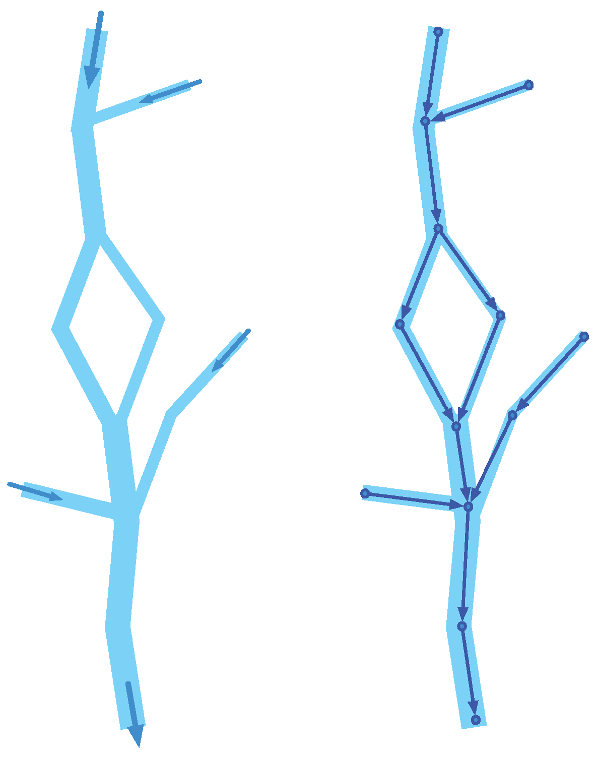
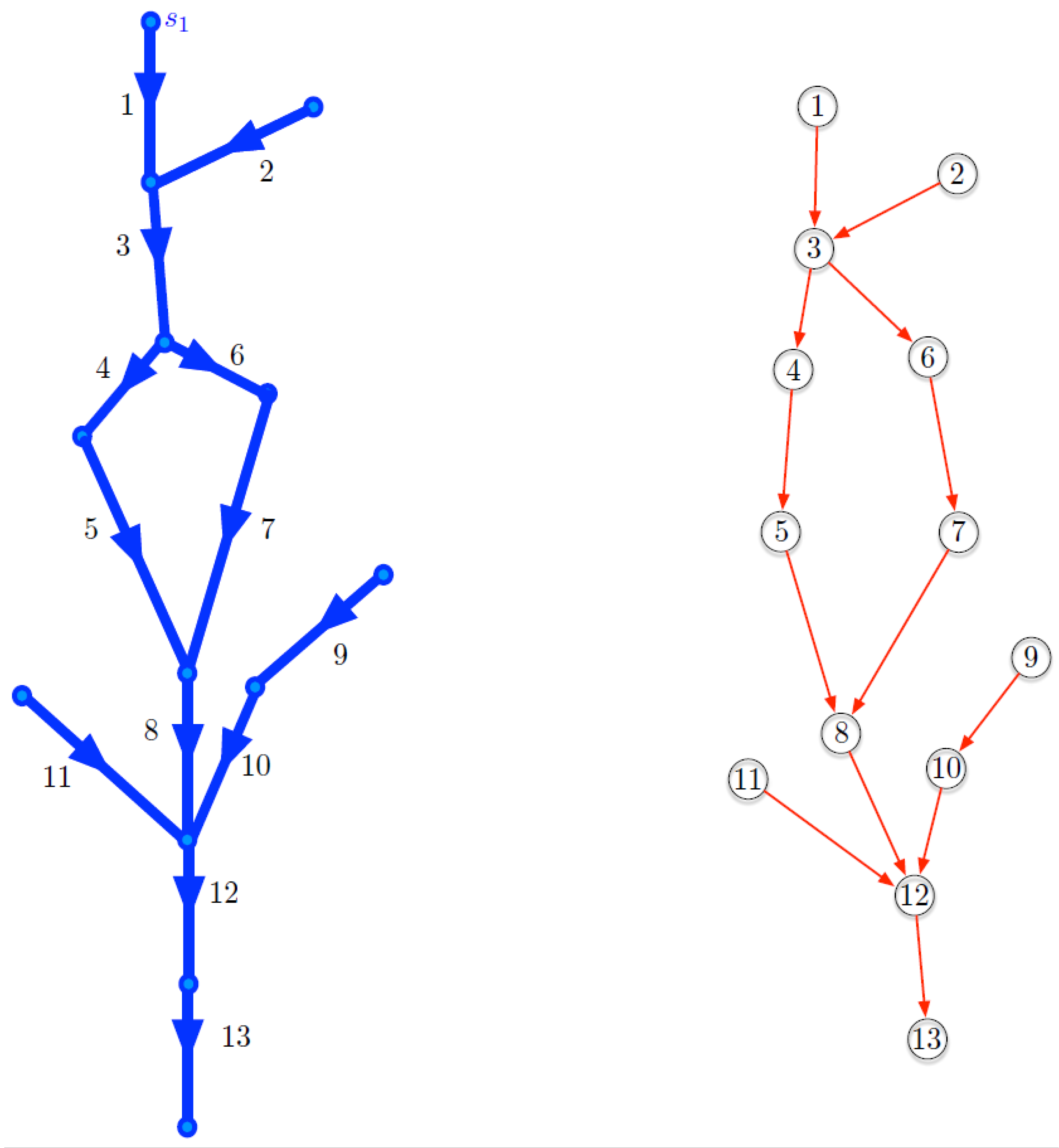
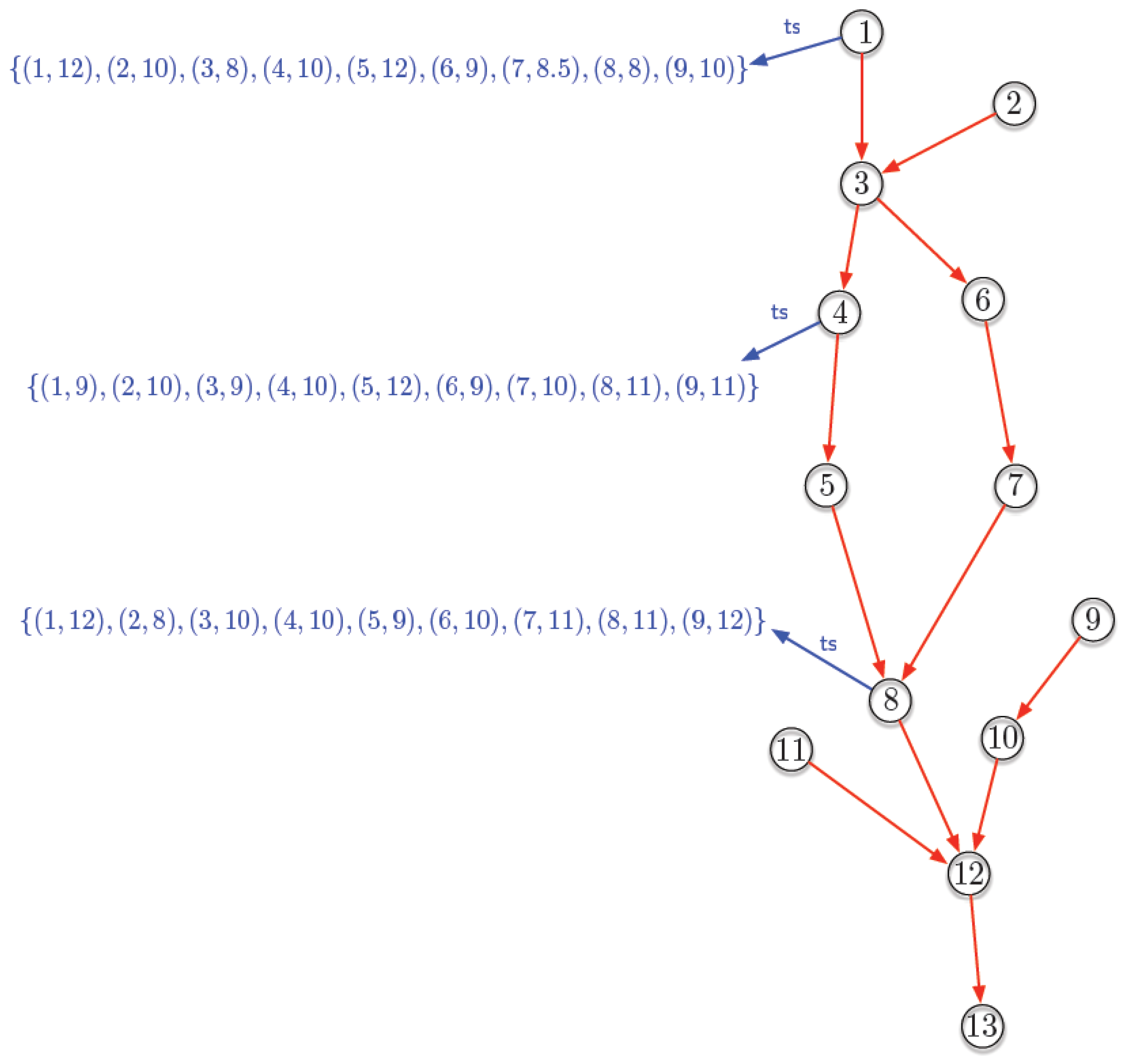
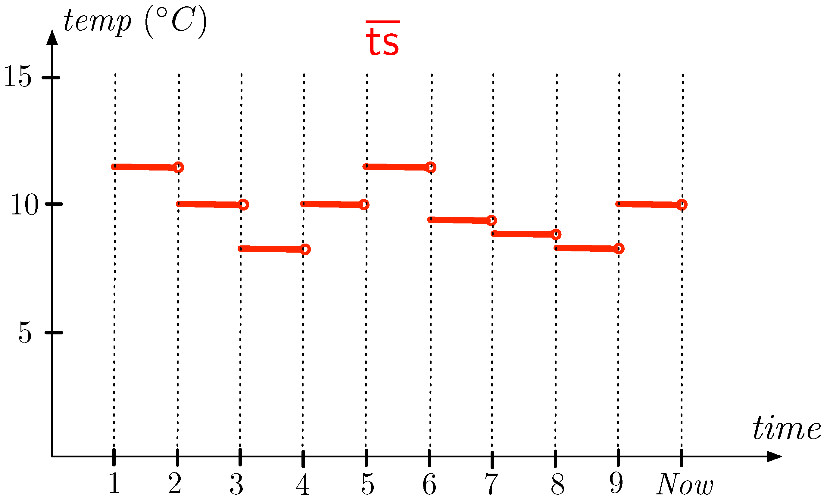
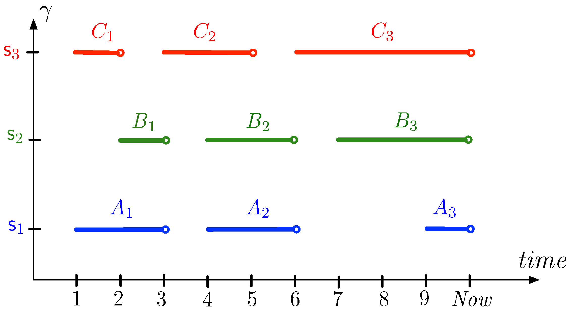
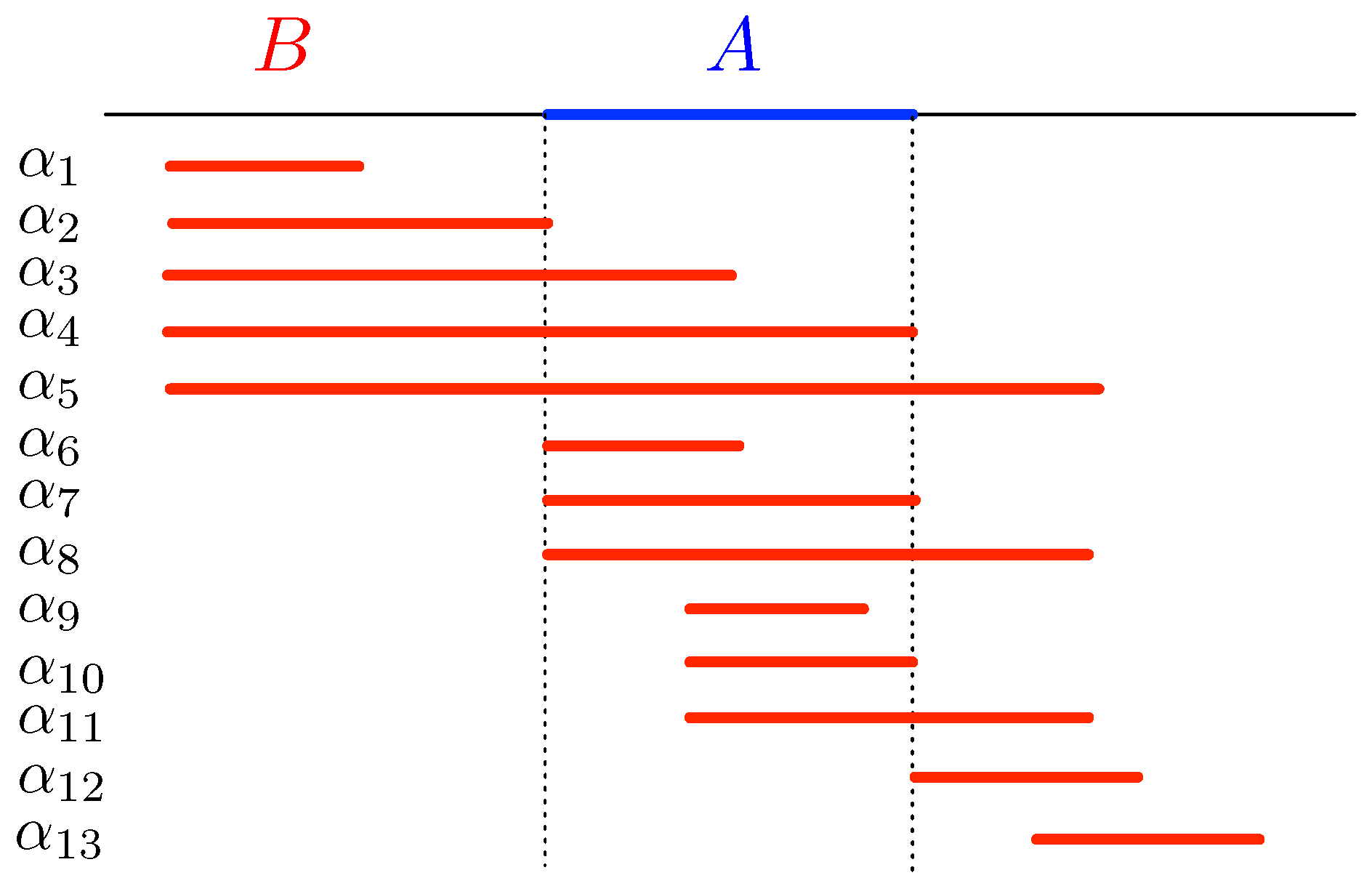
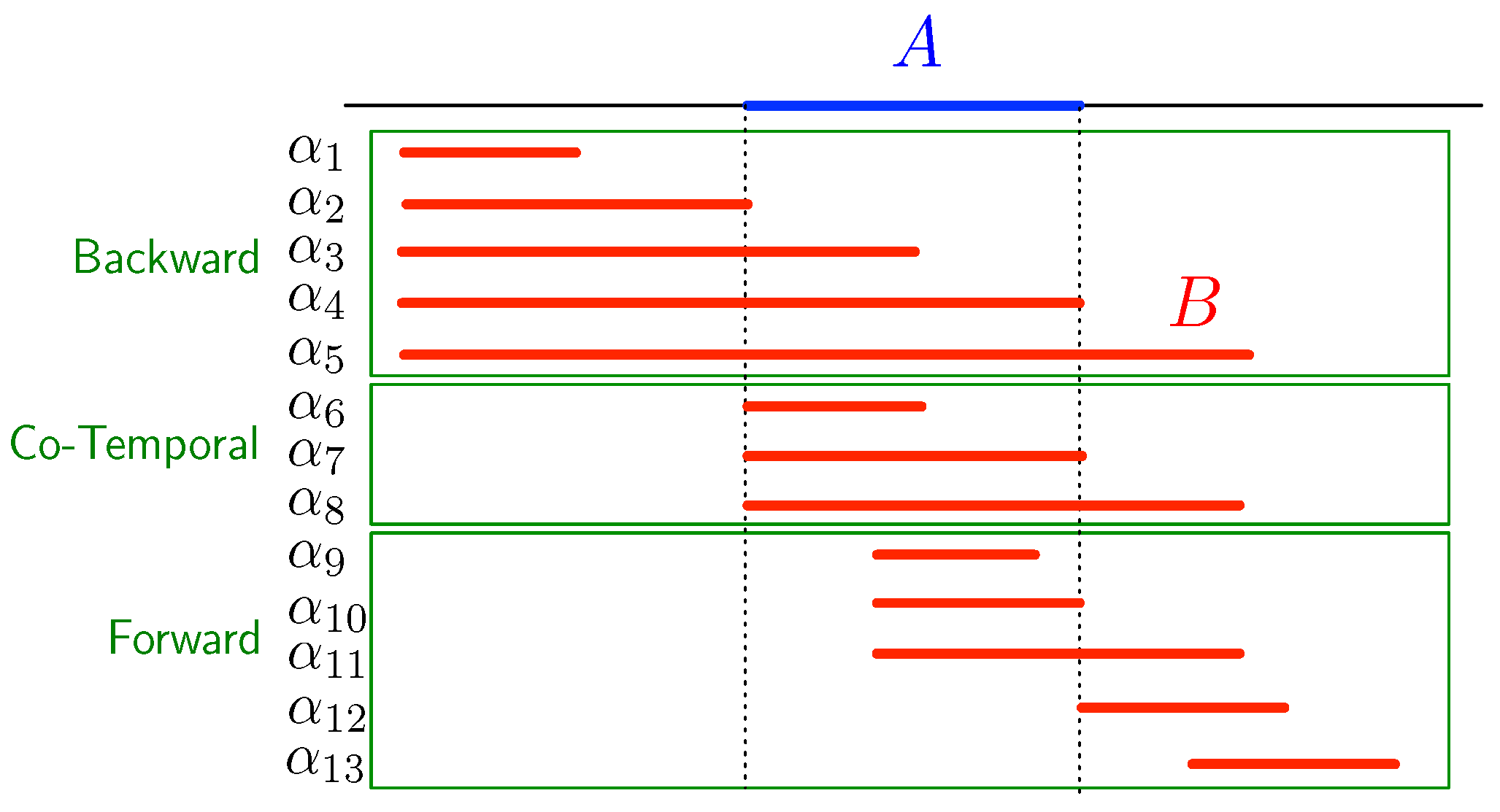
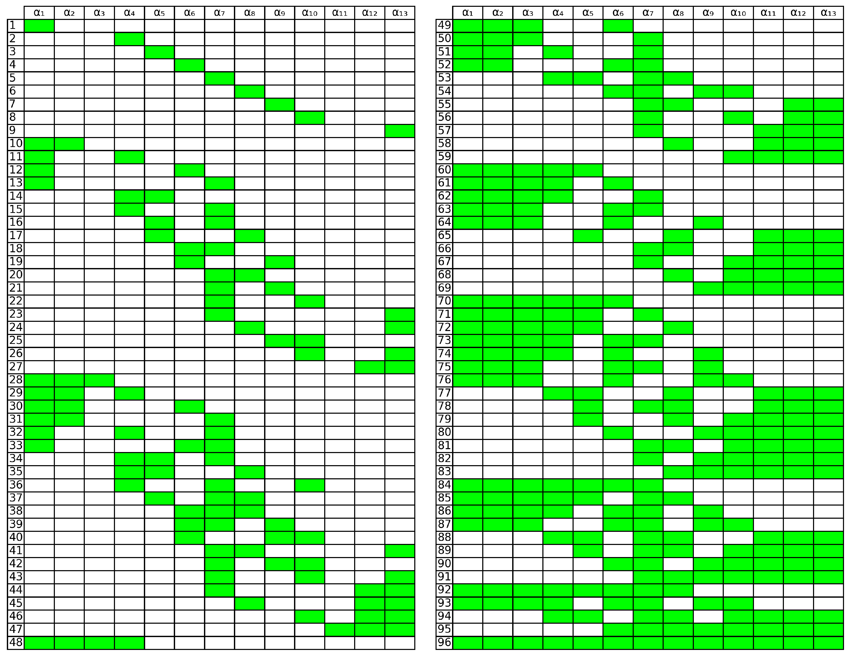
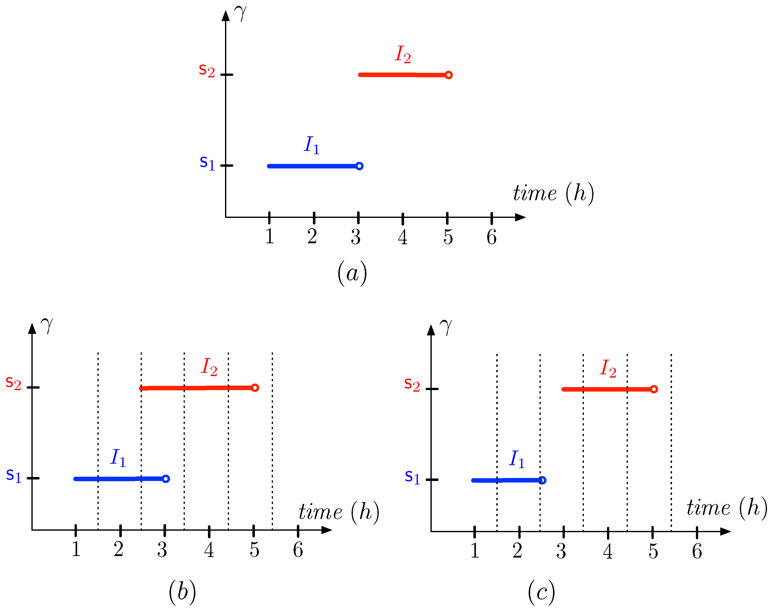
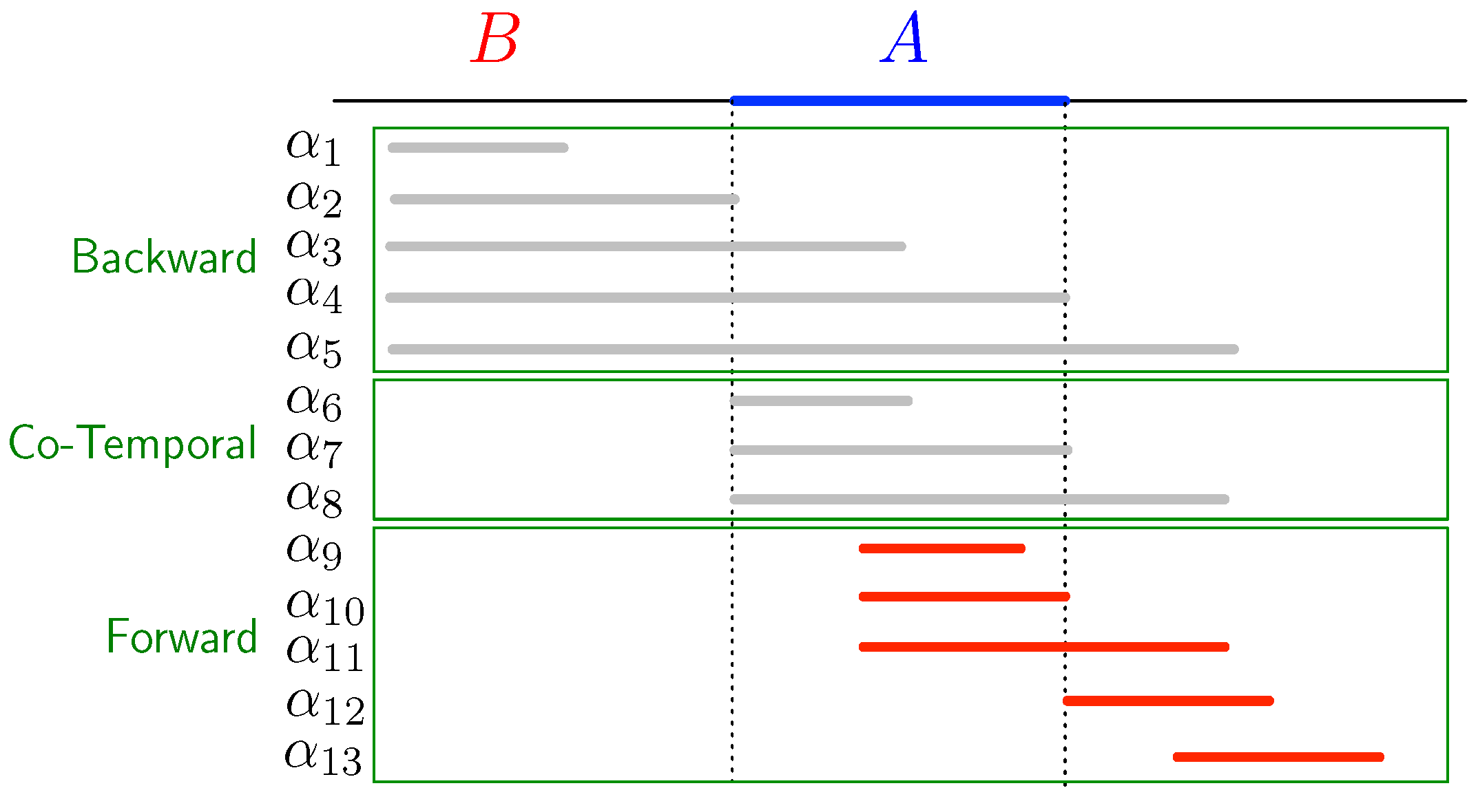
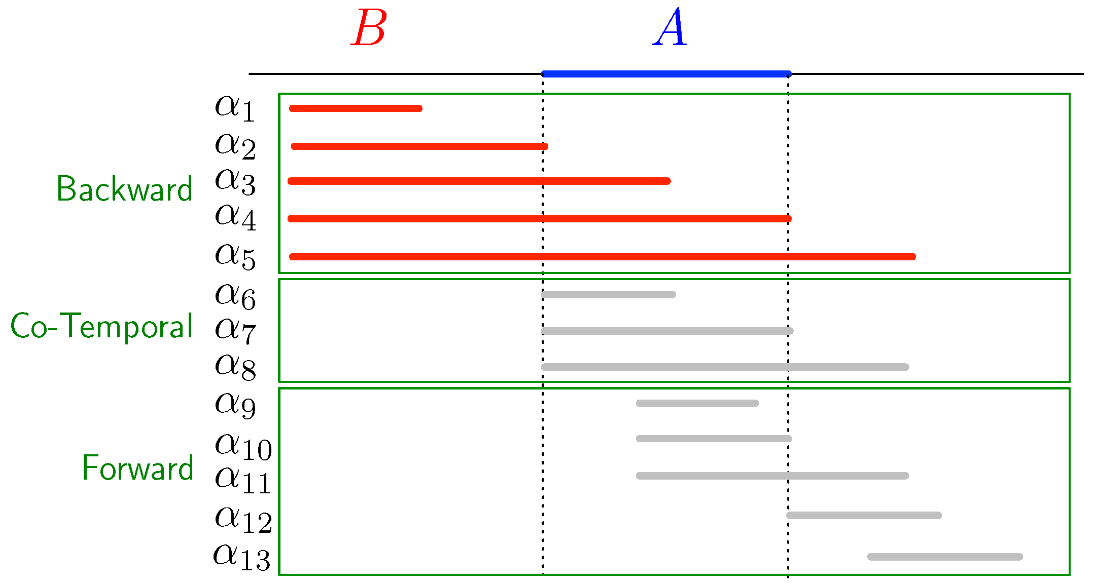
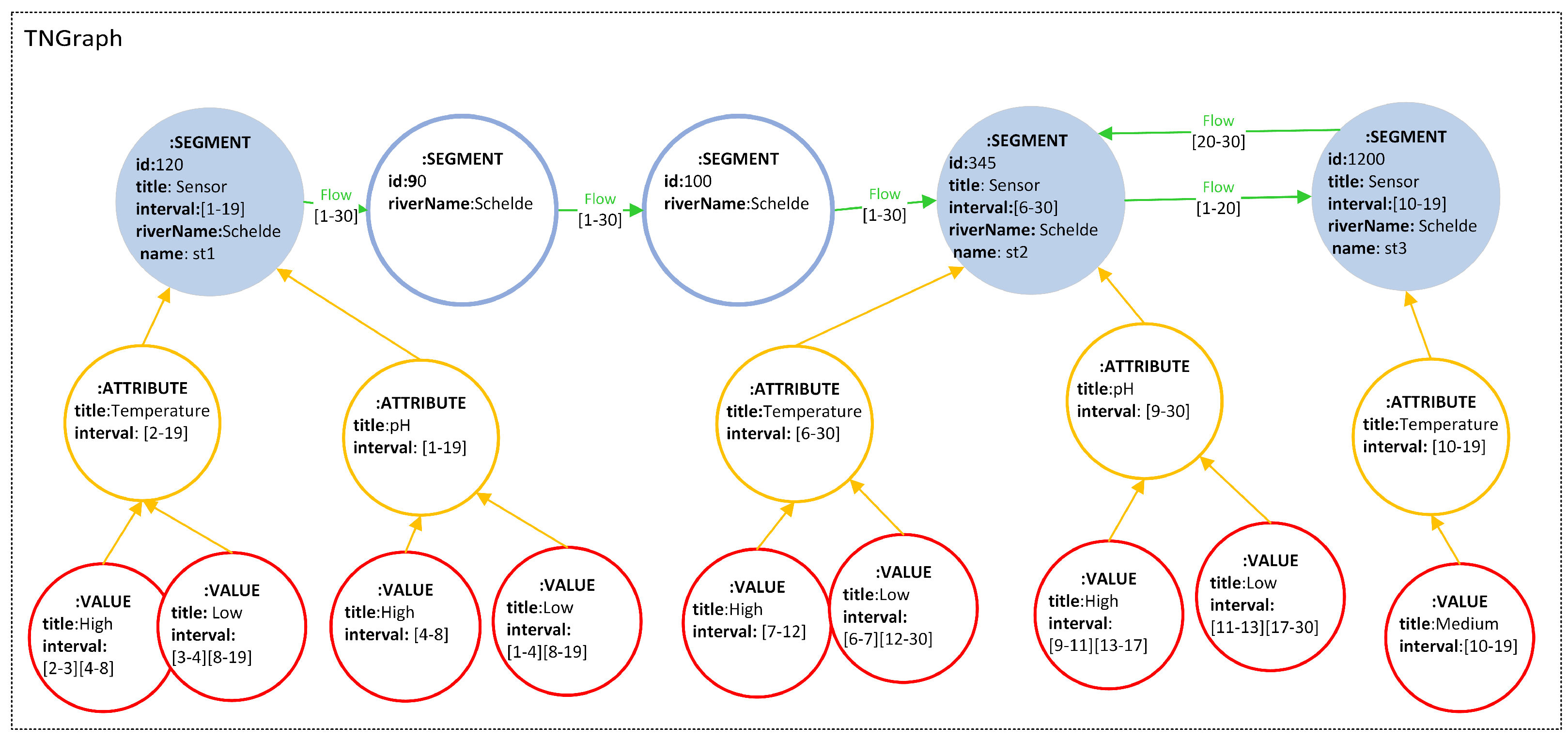
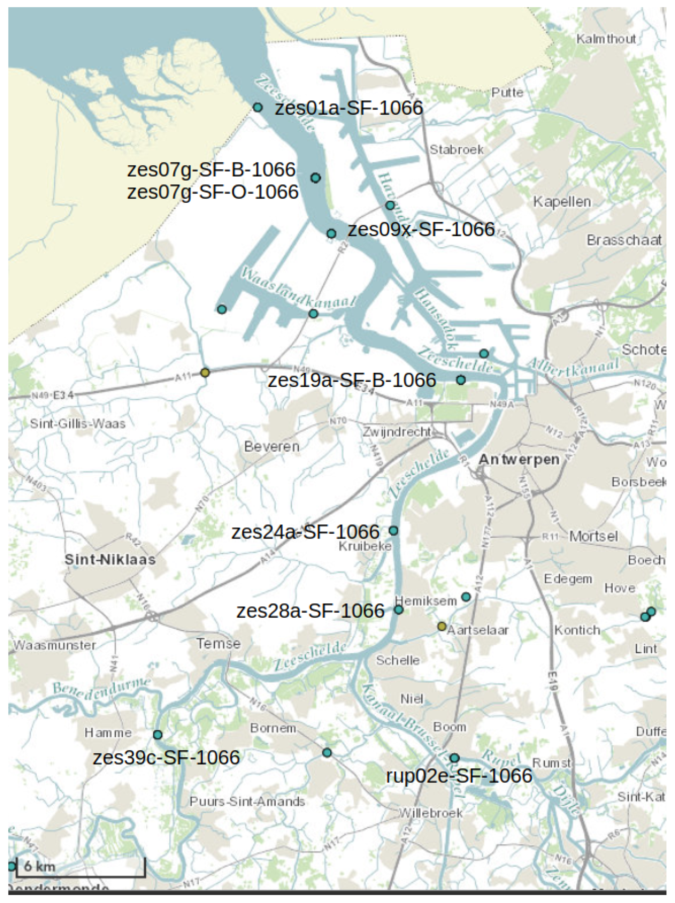
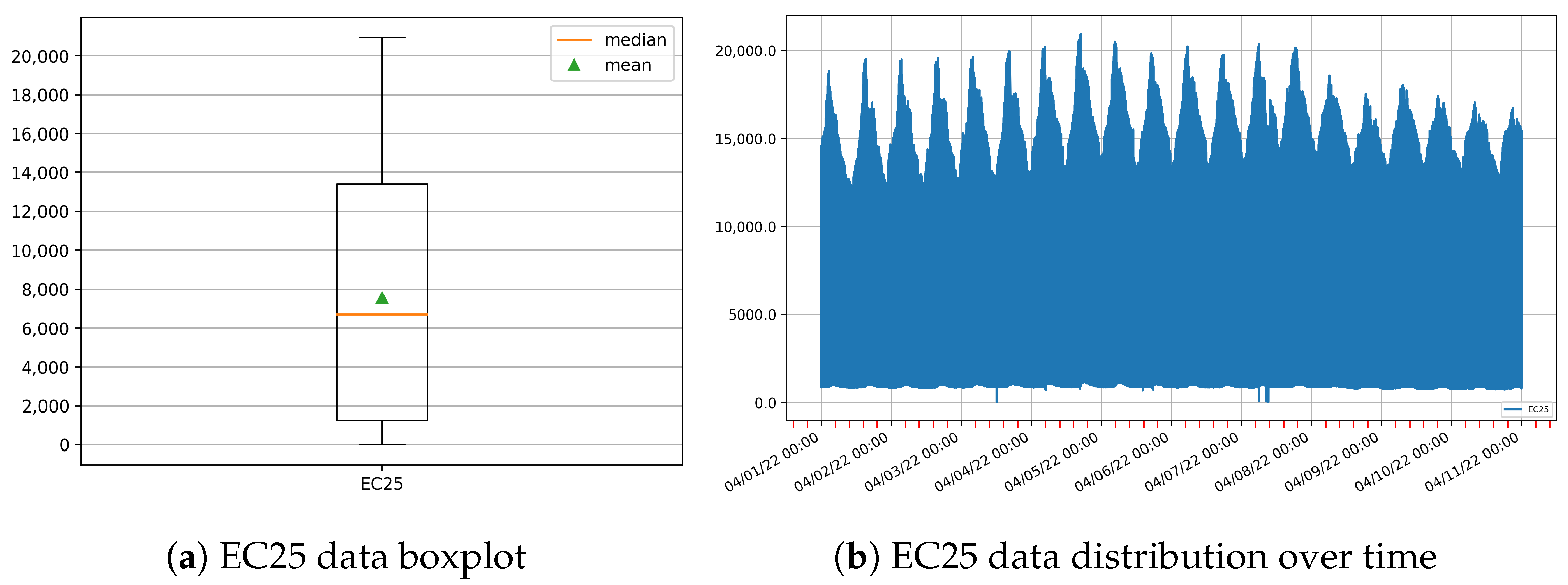
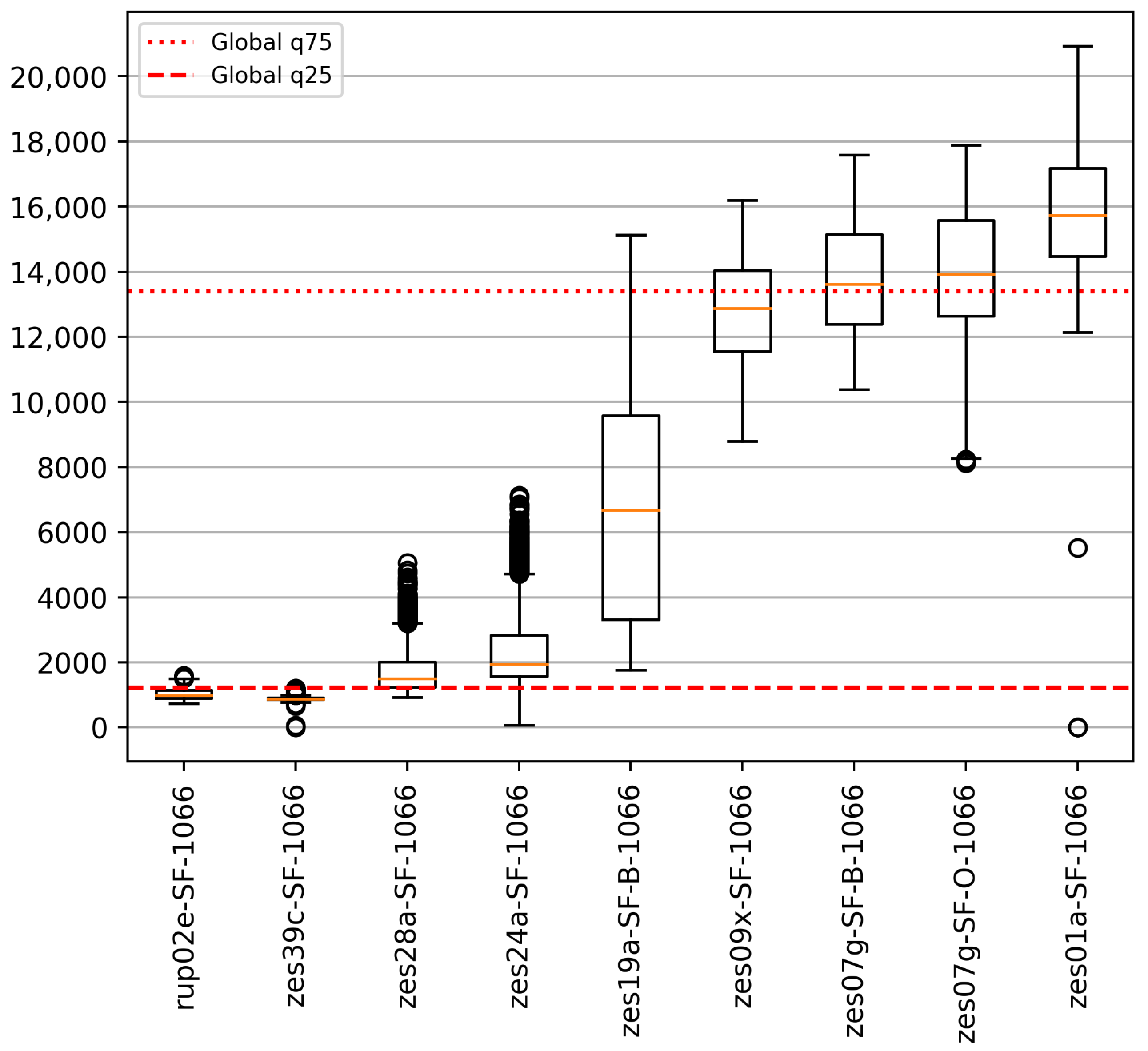
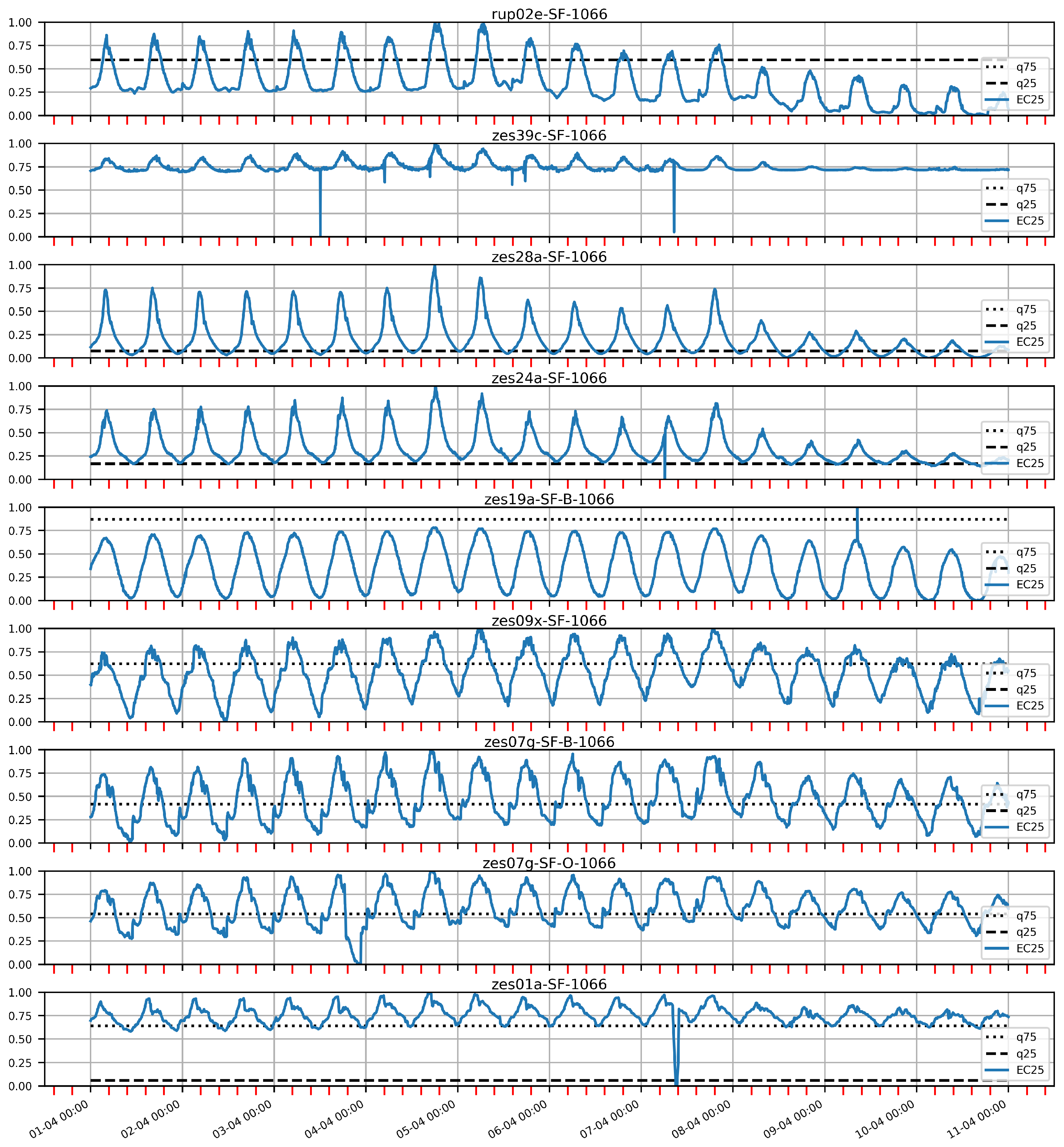
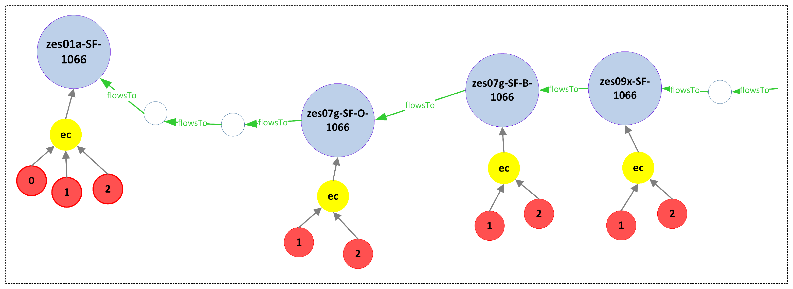
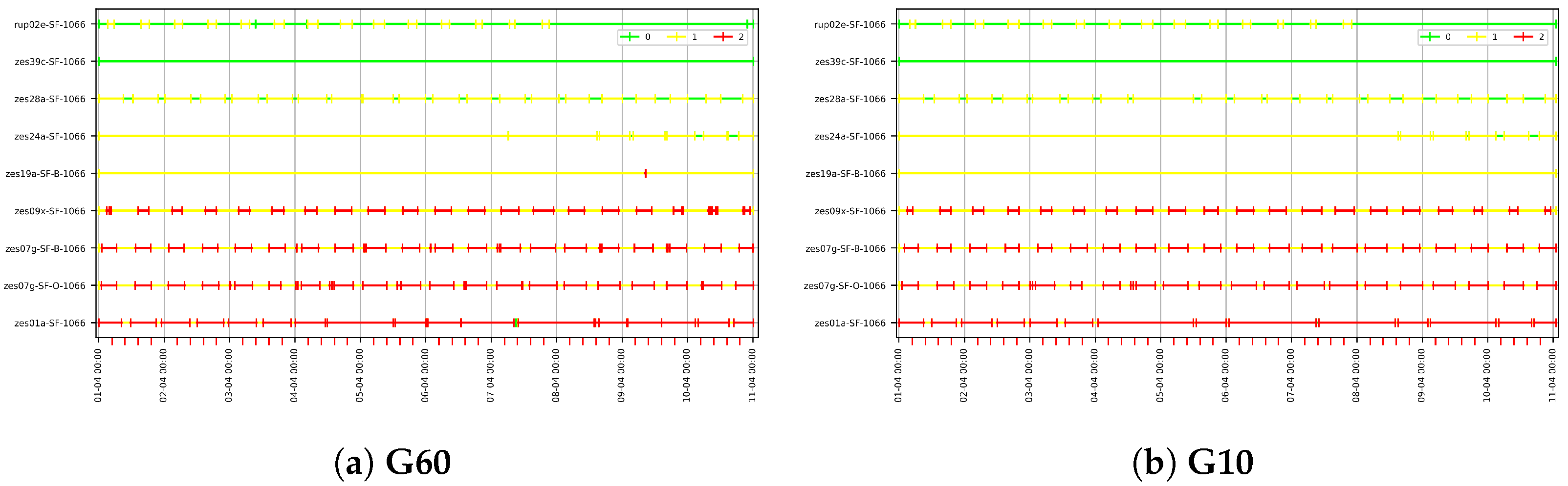
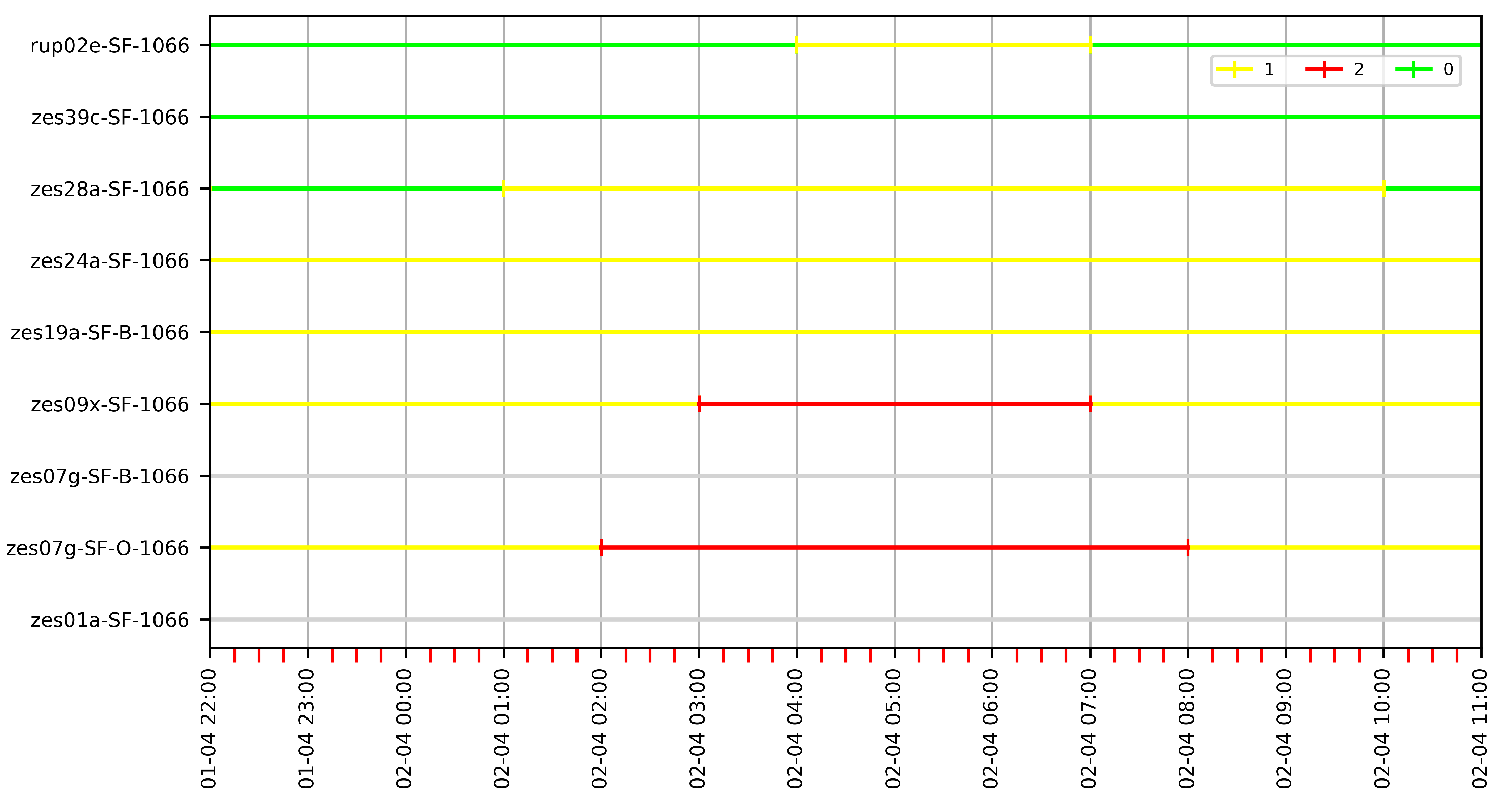
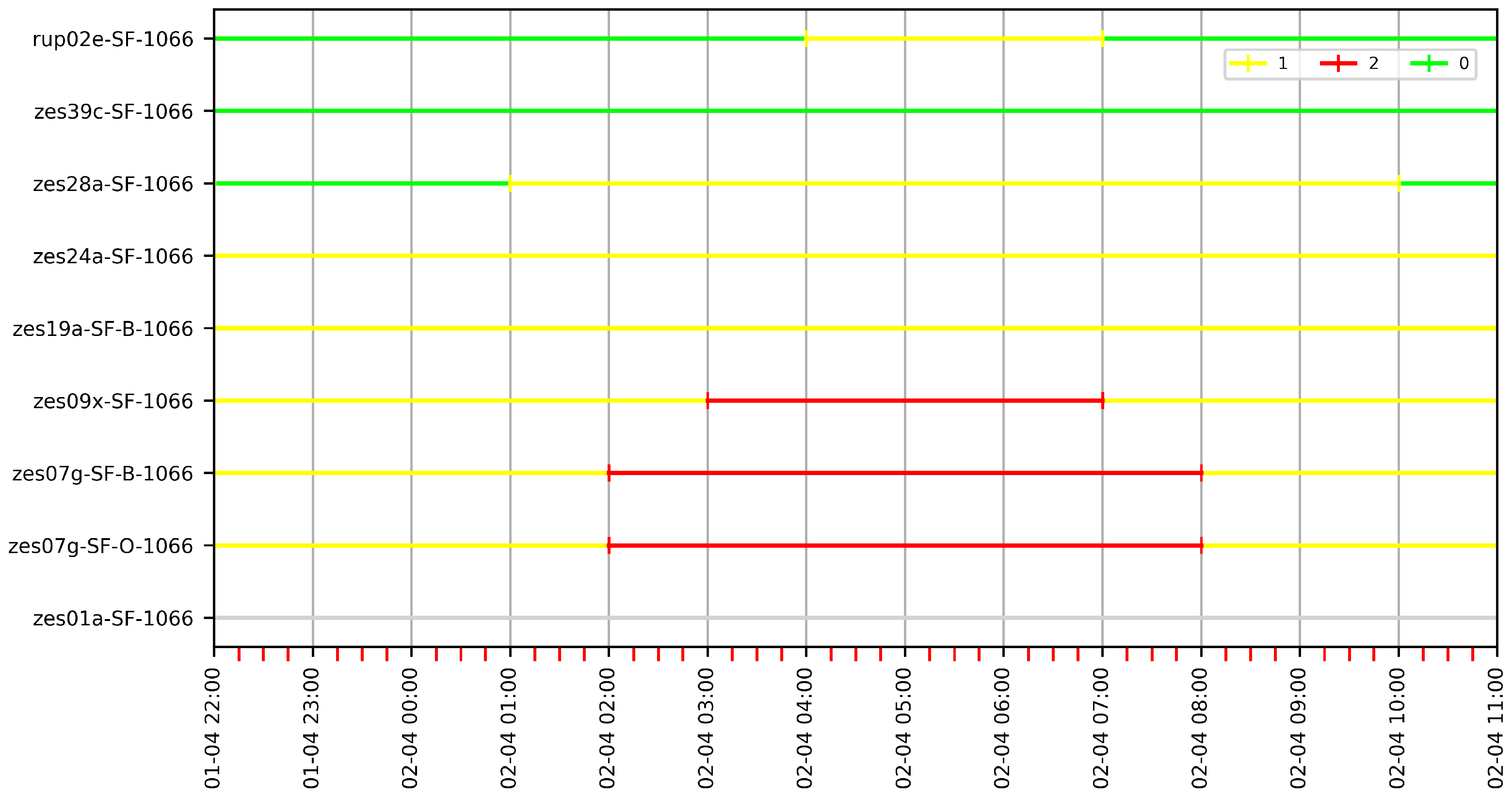
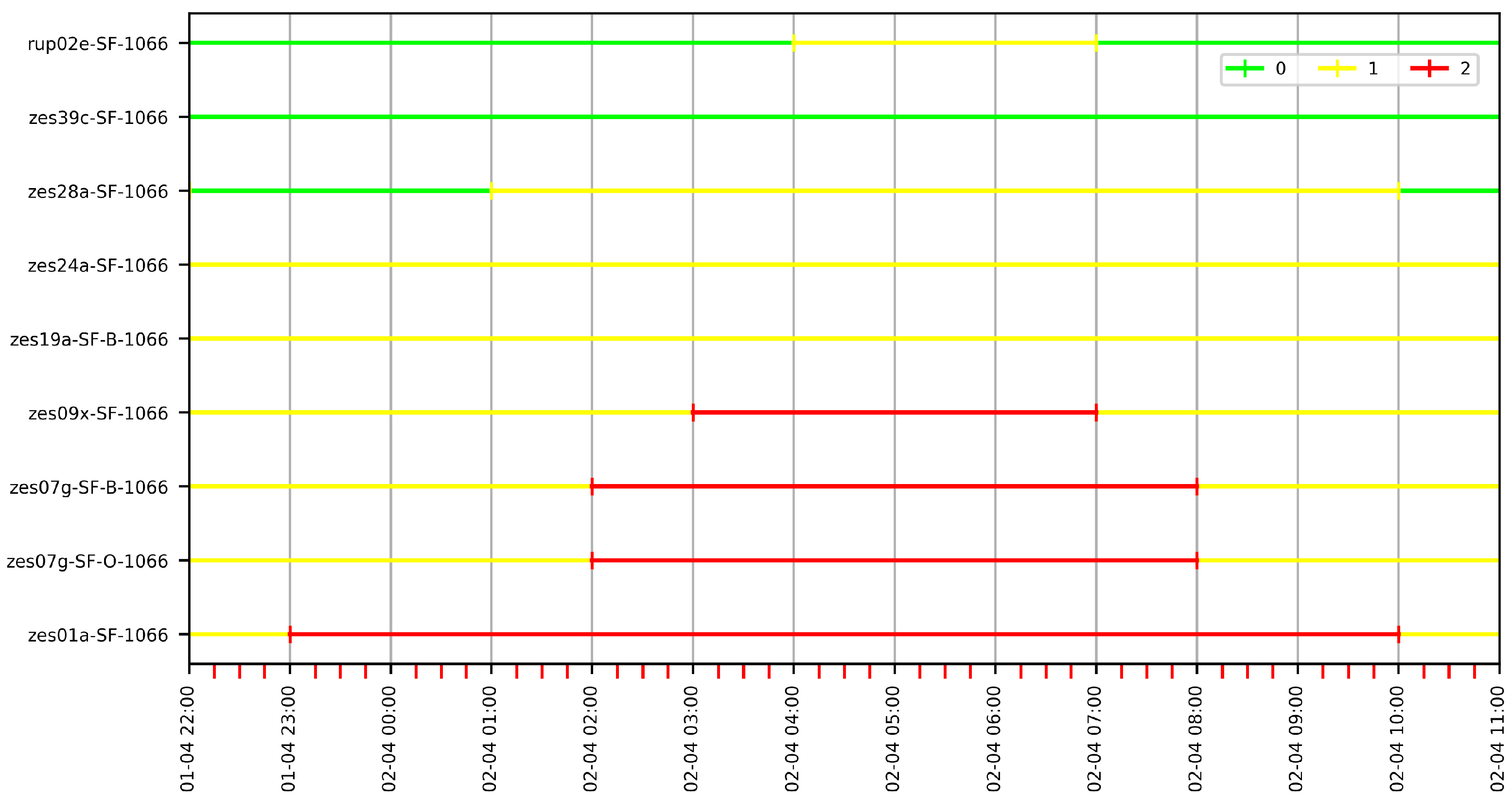
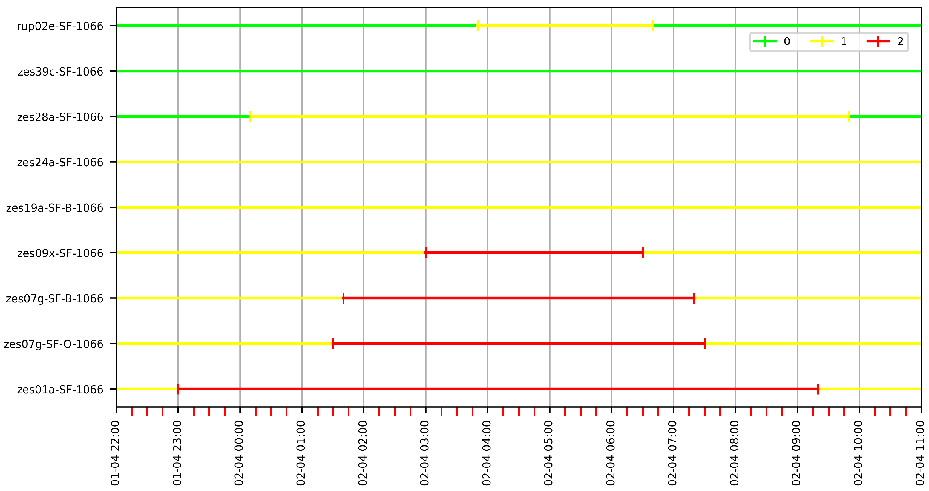
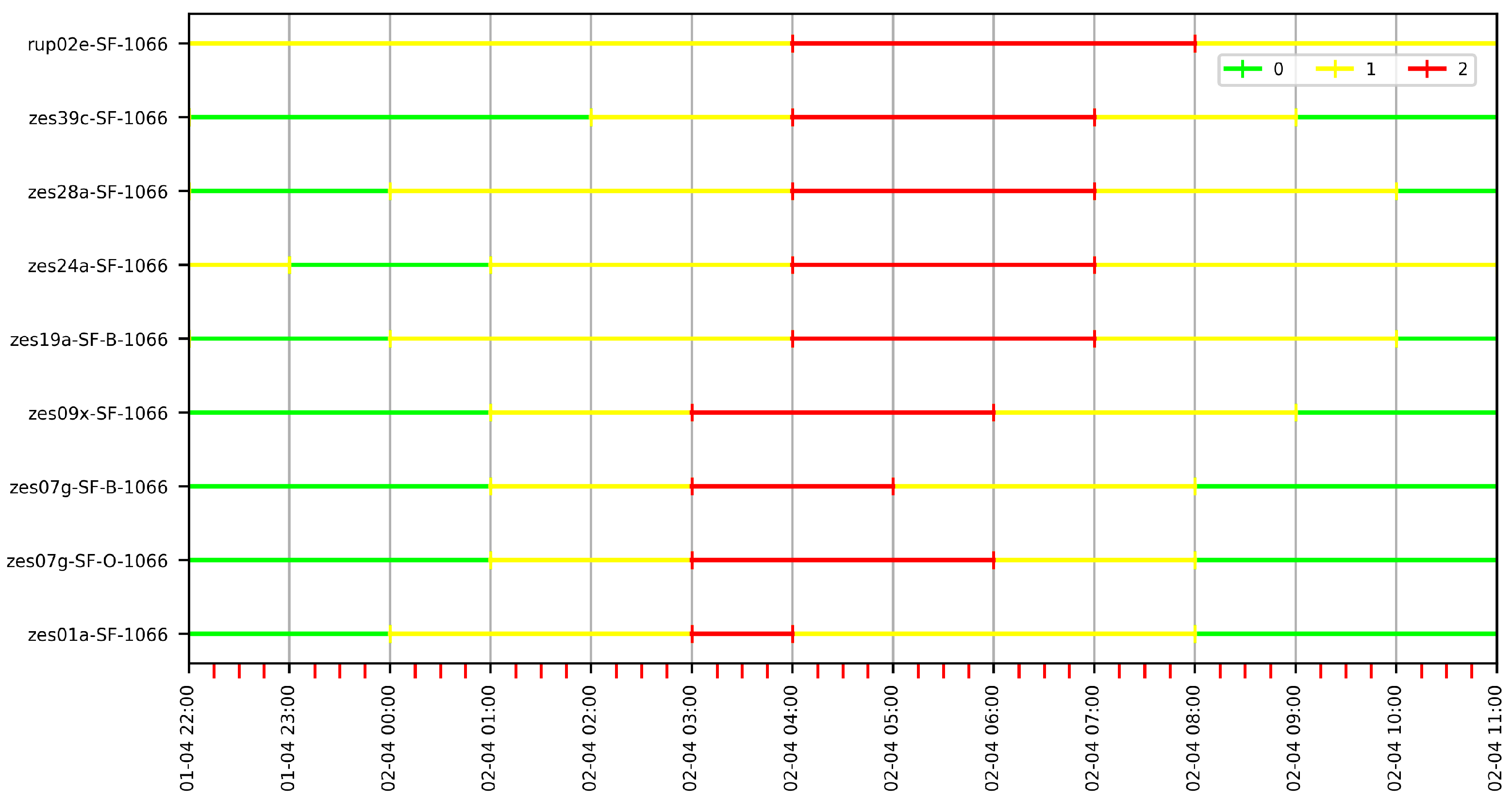
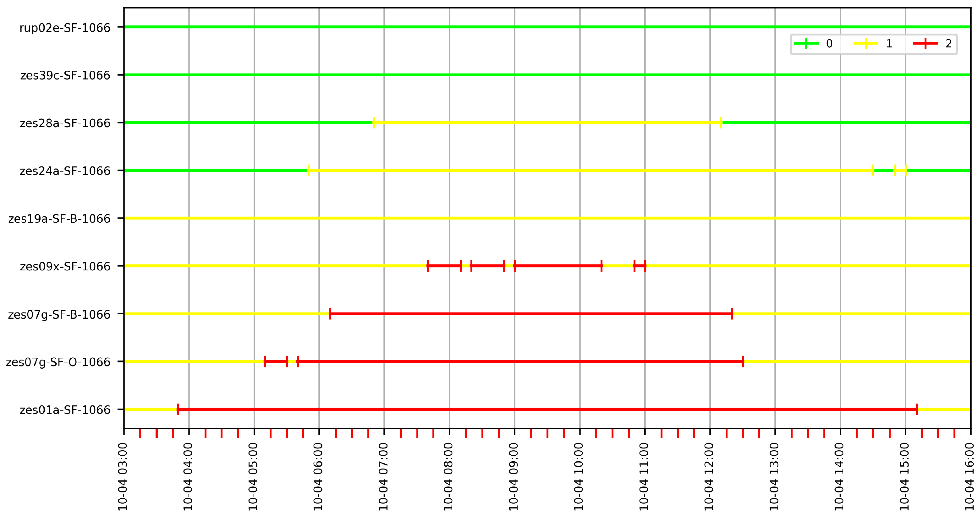
Table 1.
The traditional names of the Allen relations .
| α1 | α2 | α3 | α4 | α5 | α6 | α7 | α8 | α9 | α10 | α11 | α12 | α13 |
| > | f | d | = | s | o | m | < |
Table 2.
Closure under sensor deletion for the individual Allen relations . Green indicates closed and red not closed.
Table 2.
Closure under sensor deletion for the individual Allen relations . Green indicates closed and red not closed.
| α1 | α2 | α3 | α4 | α5 | α6 | α7 | α8 | α9 | α10 | α11 | α12 | α13 |
Table 3.
The robustification rules (going to finer granularity).
| If Contains | Then Add |
|---|---|
Table 4.
The robustification rules (going to coarser granularity).
| If Contains | Then Add |
|---|---|
Table 5.
In the horizontal lines, the eleven elements of the Allen interval algebra that are both closed under sensor deletion and robust. The presence of is indicated by a green box.
Table 5.
In the horizontal lines, the eleven elements of the Allen interval algebra that are both closed under sensor deletion and robust. The presence of is indicated by a green box.
Table 6.
EC25 variable: basic statistics. All values in µS/cm, except for the count.
| Count | Mean | Std | Min | Max | |||
|---|---|---|---|---|---|---|---|
| 23,040.00 | 7546.45 | 6094.66 | 0.00 | 1241.99 | 6687.50 | 13,398.63 | 20,927.82 |
Table 7.
EC25 variable: data description per station (values in µS/cm).
| Station | Count | Mean | Std | Min | Max | |||
|---|---|---|---|---|---|---|---|---|
| rup02e-SF | 2877 | 1032.87 | 193.57 | 736.78 | 900.89 | 983.70 | 1144.00 | 1584.71 |
| zes39c-SF | 2881 | 900.58 | 66.19 | 0.00 | 860.52 | 874.10 | 920.28 | 1200.97 |
| zes28a-SF | 1441 | 1763.52 | 763.86 | 935.04 | 1226.06 | 1499.86 | 2017.72 | 5065.56 |
| zes24a-SF | 2881 | 2395.72 | 1195.10 | 72.48 | 1566.20 | 1940.65 | 2828.31 | 7131.11 |
| zes19a-SF | 2881 | 6603.10 | 3244.00 | 1770.38 | 3316.37 | 6684.05 | 9581.82 | 15,129.36 |
| zes09x-SF | 2881 | 12,761.96 | 1644.52 | 8797.00 | 11,555.18 | 12,864.50 | 14,044.24 | 16,198.29 |
| zes07g-SF-O | 2881 | 14,068.21 | 1806.03 | 8117.48 | 12,640.51 | 13,920.28 | 15,569.23 | 17,895.11 |
| zes07g-SF-B | 2881 | 13,795.87 | 1645.01 | 10,387.20 | 12,388.06 | 13,613.61 | 15,147.64 | 17,590.14 |
| zes01a-SF | 1436 | 15,872.93 | 2035.35 | 2.81 | 14,469.30 | 15,733.44 | 17,181.65 | 20,927.82 |
Disclaimer/Publisher’s Note: The statements, opinions and data contained in all publications are solely those of the individual author(s) and contributor(s) and not of MDPI and/or the editor(s). MDPI and/or the editor(s) disclaim responsibility for any injury to people or property resulting from any ideas, methods, instructions or products referred to in the content. |
© 2024 by the authors. Licensee MDPI, Basel, Switzerland. This article is an open access article distributed under the terms and conditions of the Creative Commons Attribution (CC BY) license (https://creativecommons.org/licenses/by/4.0/).
Share and Cite
MDPI and ACS Style
Bollen, E.; Kuijpers, B.; Soliani, V.; Vaisman, A. Temporal Paths in Real-World Sensor Networks. ISPRS Int. J. Geo-Inf. 2024, 13, 36. https://doi.org/10.3390/ijgi13020036
AMA Style
Bollen E, Kuijpers B, Soliani V, Vaisman A. Temporal Paths in Real-World Sensor Networks. ISPRS International Journal of Geo-Information. 2024; 13(2):36. https://doi.org/10.3390/ijgi13020036
Chicago/Turabian StyleBollen, Erik, Bart Kuijpers, Valeria Soliani, and Alejandro Vaisman. 2024. "Temporal Paths in Real-World Sensor Networks" ISPRS International Journal of Geo-Information 13, no. 2: 36. https://doi.org/10.3390/ijgi13020036
Note that from the first issue of 2016, this journal uses article numbers instead of page numbers. See further details here.