

A Lightweight Approach for Building User Mobility Profiles
by
 , , and
Sebastián Vallejos
1,2,
Luis Berdun
1,2,
Marcelo Armentano
1,2,
Silvia Schiaffino
1,2 and
Daniela Godoy
1,2,* 1
Facultad de Ciencias Exactas, Instituto Superior de Ingeniería de Software (ISISTAN), Universidad Nacional del Centro de la Provincia de Buenos Aires (UNCPBA)—Consejo Nacional de Investigaciones Científicas y Técnicas (CONICET), Tandil 7000, Buenos Aires, Argentina
2
Instituto Superior de Ingeniería de Software (ISISTAN), Universidad Nacional del Centro de la Provincia de Buenos Aires (UNCPBA)—Consejo Nacional de Investigaciones Científicas y Técnicas (CONICET), Tandil 7000, Buenos Aires, Argentina
*
Author to whom correspondence should be addressed.
ISPRS Int. J. Geo-Inf. 2024, 13(1), 11; https://doi.org/10.3390/ijgi13010011
Submission received: 7 October 2023
/
Revised: 21 December 2023
/
Accepted: 23 December 2023
/
Published: 27 December 2023
Abstract
:Data captured by mobile devices enable us, among other things, learn the places where users go, identify their home and workplace, the places they usually visit (e.g., supermarket, gym, etc.), the different paths they take to move from one place to another and even their routines. In summary, with this information, it is possible to learn a user mobility profile. In this work, we propose a lightweight approach for building mobility profiles from data collected with mobile devices. The mobility profiles of a user consist of the places visited, the visit history and the travel paths. Our approach aims to solve some of the challenges and limitations identified in the literature. Particularly, it considers geographic information to identify certain kinds of places, such as open spaces, big places and small places, that are hard to distinguish with existing approaches. We use different sensors and time frequencies to collect data in order to optimize battery consumption and maximize precision. Finally, it executes entirely on the mobile devices, avoiding the exposure of sensitive user information and then preserving user privacy. The proposal was evaluated in the context of the real usage of the developed prototype applications in two cities of Argentina. The results obtained with our approach outperformed other approaches in the literature, both in precision and recall.
1. Introduction
In the last few years, mobile devices have taken a very important role in our lives. Almost everyone owns a personal mobile device that they carry with them all the time. Particularly in Argentina, 91% of the population owned at least one mobile device in 2017 [1].
Over the years, these devices have acquired great processing capacity, allowing a large amount of data to be processed and stored. In addition, they come equipped with a wide variety of sensors capable of capturing and recording different types of data in a non-intrusive way. The availability of these data opened the doors to a world of possibilities and, in particular, made it possible to study users’ mobility [2]. By analyzing the data generated by a mobile device, it is possible to learn different aspects of users’ mobility, such as the places visited, the routes taken to reach them and the activity carried out in those places. These data allow the construction of user mobility profiles [3,4], which are useful both at the individual level, for the development of context-sensitive services [5,6] and at the group level, in the context of smart cities and tourism [7,8,9].
At an individual level, a user mobility profile enables the development of applications and services to assist users in their daily routine. User profiles have been widely used by systems that take into account the particular characteristics of people, including their habits and interests, to offer assistance and personalized recommendations in different domains [5,10,11] and for the development of multiple applications [12,13]. At a group level, the mobility profiles of all citizens would provide valuable information about the urban mobility of a city [14,15]. For example, we could learn about the mobility of citizens in the city or how they use public transportation and public spaces [16].
Different authors have studied the use of data captured by mobile devices for learning user mobility. However, after a systematic analysis of the literature, we observed that there are problems that have not yet been addressed or that need to be studied in greater depth. In the first place, most of the studies propose approaches that do not consider the privacy problems involved in exposing sensitive user data [17], such as their geographical location and the information about the places they visit. Second, existent approaches use static parameters for the detection of stays and places. The use of static parameters implies serious limitations to the correct identification of places with different dimensions, since parameters that are well suited to small places (such as a house) often present problems when the user visits larger places (such as parks, supermarkets or warehouses). Third, there is a lack of datasets suitable for evaluating the different techniques proposed for detecting visits and places. This is due to the difficulty of building a detailed dataset, since users consider it a very time-consuming task to keep a daily record of all their movements. At the same time, datasets are rarely available to the scientific community due to the previously mentioned privacy concerns. In this sense, many authors have used geo-localized public content extracted from social networks, especially check-ins made by users [18,19,20], data from location-based services [21], trajectory datasets such as GeoLife (https://www.microsoft.com/en-us/research/publication/geolife-gps-trajectory-dataset-user-guide/, accessed on 1 July 2023) and tracking datasets [22]. However, these data are not representative or useful for our purposes, since it is not possible to know how much time users spent in each place (stays cannot be detected), in addition to the fact that users usually skip checking in in everyday places (such as home or work). For example, the Geolife dataset contains trajectories, i.e., routes defined by a sequence of points, but it does not contain information about the places visited (the stays that are recognized as places). This dataset contains trajectories from 182 different users but presents many data gaps (the focus of the dataset is on the trajectories and not on mobility patterns of individuals). Some authors [23] suggested that only users with more complete data should be considered. For our purposes, to identify a user stay (i.e., areas where the user stopped for a certain amount of time), we require that the end of a trajectory matches the beginning of the next trajectory. Only six users of the Geolife dataset could have been considered.
In this work, we propose a lightweight approach for the construction of mobility profiles from the data collected from sensors in the users’ mobile devices. A mobility profile consists of the places visited by the user and the visits history, i.e., when each visit begins and ends and the roads the user takes to get from one place to another (the travel path). The proposed approach seeks to solve some of the problems and limitations identified in the literature mentioned above. The approach has two main components in charge of carrying out the most important stages in this scenario: the collection of data from the different sensors of the device and the processing of the data collected to detect stays, trips and places visited by the user. Then, this knowledge could be used to learn patterns in the users´ mobility that allow predicting the next destinations they will visit. All the components run entirely on users’ mobile devices, thus avoiding exposing any sensitive data that could compromise their privacy. Special attention when developing our approach was put into optimizing battery usage. Since the app is running continuously on the user’s mobile phone (we have to gather the user’s location constantly), it is crucial to limit location requests as much as possible and also to choose the method for identifying it (GPS or Wi-Fi).
The proposed approach was evaluated using two prototype applications named Asistan (https://play.google.com/store/apps/details?id=ar.edu.unicen.isistan.asistan (accessed on 15 December 2023)) and APS (https://play.google.com/store/apps/details?id=ar.edu.unicen.isistan.ayacucho (accessed on 15 December 2023)) developed for this purpose. The experiments carried out aimed at evaluating different aspects of the proposal. First, we evaluated the ability of the approach to identify and discard wrong or deviated locations. Then, we evaluated the ability of the approach to detect users’ stays and places visited. The results obtained are promising since our proposal outperformed other approaches in the literature.
The main contributions of this approach are:
- An adaptive battery-friendly data collection method that uses different localization mechanisms (GPS, WiFi, GSM) with different frequencies according to the user’s current context.
- The use of volunteers geographic information and discovered user’s personal places to automatically adapt the parameters for the detection of stay points.
- A state machine for stay points detection capable of running in a user’s mobile device in an online manner and able to withstand situations of uncertainty.
The rest of the article is organized as follows. In Section 2, we discuss some basic concepts and related works. In Section 3, we present our proposal. Then, in Section 4, we describe the experiments we carried out to evaluate our approach and the results obtained. Finally, in Section 5, we discuss our conclusions and present some future research lines.
2. Background and Related Works
Works seeking to take advantage of the data provided by mobile devices to extract information about the daily mobility of people and their routines, which generally involves two main stages, are detailed in the following sections. The first stage consists of collecting the data generated by the different sensors of the mobile devices (Section 2.1), whereas the second stage is in charge of processing the data collected to identify the different places the user visited and extract the history of visits and trips made (Section 2.2).
2.1. Data Collection
In the study of urban mobility, perhaps one of the most important types of data to collect is the location of the user. However, the geographical location of people needs to be associated with the activity carried out in such a location. Combining this information, it is possible to learn about the user lifestyle and routines: knowing how many hours a day they are working or resting at home, knowing if they usually go out to eat at restaurants, if they play sports, etc.
Mobile devices come equipped with various sensors and radios that allow us to estimate a user’s current location. Location by GSM (Global System for Mobile communications) allows locating a device from the cell towers that surround it. Mobile phones also have a radio for connecting to cell towers to make or receive calls and messages. Then, knowing the cell towers which are close to the device and their geographical positions, triangulation mechanisms can be used to locate the device [24]. Wi-Fi location, called WPS (Wi-Fi Positioning System), locates the device based on the Wi-Fi access points around it. Currently there are web services (e.g., the Google geolocation API https://developers.google.com/maps/documentation/geolocation/intro (accessed on 15 December 2023)) that, indicating nearby WiFi access points, estimate our geographical location from a private repository. However, it is required to have an internet connection. GPS (Global Positioning System) location consists of locating a device at some point on the Earth’s surface from a set of satellites around the Earth. This strategy determines the distance between the device and a group of satellites. Inverse trilateration is used to estimate the geographical coordinates of the receiver. Currently, almost all mobile devices on the market have a GPS receiver for this purpose. GPS location can locate objects with precision between 3 and 50 m when there are no obstacles interfering with the communication between the mobile device and the satellites [25].
Different strategies have been proposed in the literature to know the user’s location precisely and reduce the negative impact on battery consumption. Table 1 shows the values reported in [26] on the accuracy and battery consumption of each mechanism as a summary. Clearly, there is a trade-off between the precision in localization and the energy consumption. To avoid privacy concerns in [27,28], the authors made use of CDRs to infer users locations and crowd-sourced geospatial information to characterize and explain the locations. However, the approach needs to have access to the mobile companies data and the precision of the inferred location has lower quality when compared to GPS. Furthermore, CDRs might not fully represent human mobility as they are only produced when individuals engage with the mobile network. Furthermore, the precision of data gathered from crowdsourcing fluctuates based on the extent of participation and the quality of information provided by the users. This approach could be a good option to analyze the mobility of a population as a group, but the individual mobility could have several challenges, for example, how to determine the road used by the user to commute from location A to location B.
Adaptive strategies have been proposed to deal with this trade-off by establishing the localization frequency and mechanism according to the situation. In the case of location frequency, it can be reduced when the user location does not change (e.g., when the user is not moving). In [32,33,34], the authors use the accelerometer to detect whether the user is moving or not for this purpose. Regarding the localization mechanism, works in the literature usually propose a combination of different mechanisms, considering their advantages and disadvantages [32,35,36,37].
In [32], the authors select the mechanism of localization according to the user state. While the user is traveling, the GPS location is used. Instead, when the user reaches the destination, Wi-Fi location is employed. This methodology reduced battery consumption by 87% compared to using GPS alone. However, the disadvantage is that precision is lost when the user stops in one place outdoors or with few nearby WiFi hot-spots. In [36], the authors seek to reduce the battery consumption using WiFi location whenever possible, but when it becomes inaccurate or unavailable, it is replaced by GPS location. Conversely, in [38], the authors always prioritize the use of GPS location, which is only replaced by Wi-Fi when the GPS location has signal reception problems (indoors). This strategy seeks to always collect the most accurate data available at the cost of increasing battery consumption.
Modern mobile devices are equipped with different sensors that allow estimating the physical activity of the user. Different sensors have been used in the literature to infer the current activity of the user. The most commonly used sensors for this purpose are the accelerometer and the gyroscope. These sensors measure the acceleration forces and the speed of rotation of the device, respectively. The combination of both sensors allows us to detect any movement or change in the device. Several works in the literature used these sensors to determine the physical activity of the user: standing still, walking, running, cycling, being in a vehicle [39,40,41]. Other sensors frequently used to identify user activity are the magnetometer and the barometer. The magnetometer allows us to determine the orientation of the device with respect to the Earth’s magnetic field. Some authors found the use of this sensor useful in complement with the gyroscope and the accelerometer to infer the user’s activity [42,43,44]. Other studies used specialized devices and sensors to detect users’ locations, such as Pico Minifinders [45].
2.2. Data Processing
Data collected for a user u is generally based on a sequence of geographic positions , where each geographic position has the form of (latitude, longitude) and indicates the date and time the user was in . The objective of this stage is to process this data in order to identify the places the user visits (home, work, favorite restaurant, etc.); the user’s entrances and exits to each of these places (when each of the visits begins and ends); and the roads the user takes to travel from one place to another (the path traveled). To carry out this task, a two-stage process is carried out. In the first stage, the user’s stay points are detected. A stopover or stay point consists of a geographic area where the user stopped for a certain amount of time. When this happens, it is assumed that the user stopped there to visit the place. Then, in the second stage, the detected stay points are grouped to identify places that the user visited. In this way, from approaches, generate the set of places where each is a location that the user has visited and a sequence of visits where each visit is a triplet that indicates the visited place, the start time of the visit and the end time of the visit.
When a user visits a place, staying in that place is recorded as a sequence of geographic positions around the visited place. Formally, a stay point is a geographical area where the user stayed for more than a certain time threshold within a limited distance [4,46]. Thus, a stay point can be represented as a triplet where C is the centroid of the geographic area in which the user stayed, is the time in which the user arrived at the place and is the time at which the user left that place. In some approaches, there are no preset or values, while in others the values are established as considered convenient. For example, for some authors consider 50 m [47] while others consider 250 m [46]. However, none of the revised works addresses the possibility of using dynamic parameters.
Once the stay points have been detected, the different places visited by the user can be identified. The logic in the detection of places is that if the user frequently visits a place (e.g., the house), several stay points will be detected in the area surrounding the place. By grouping the nearby points of stay, it is possible to identify the places visited by the user. It should be noted that different previous works group the stay points at different levels of granularity, organizing them into hierarchies where several small places are inside larger ones. One of the simplest strategies is to group stay points based on the distance among them (e.g., [23,48]). The main advantages are that it has a low computational complexity and that it can be executed incrementally as the user visits different places. In [31], the authors proposed a variant of the K-means algorithm to cluster stay points. Some authors proposed to use density-based clustering algorithms (such as DBScan or DJCluster) for the same purpose [49,50,51]. In [52], the authors proposed to apply graph theory for the detection of places based on the user’s stay points.
3. Proposed Approach
In this section, we describe the approach proposed for the construction of user mobility profiles from the data collected on their mobile devices. In Section 3.1, we present an overview of our proposal. Then, in Section 3.2, we describe the component in charge of data collection, and in Section 3.3, we describe the component in charge of data processing.
3.1. General Overview
Figure 1 shows a general schema of the proposed approach, which has two components in charge of carrying out the two traditional stages for the construction of mobility profiles. The first component is responsible for data collection. The data collected enters the second component, where it is processed to detect user visits and to identify the different places visited. Then, the identified places and the detected visit history constitutes the user’s mobility profile.
The first component, responsible for data collection, collects the geographical location of the user and also the physical activity she is carrying out. As it collects data, the component adapts the collection frequency and the sensors or location mechanism used (GPS or Wi-Fi). The data collected is the input for the second component, which processes the data in order to detect user visits and to identify the different places visited. The proposed approach adapts the values of the parameters according to the context of the user. For this, the component uses geographic information from external sources, which allows it to determine when the user is visiting small places or large places (such as a park). Visits or stays detected are used to identify the places visited by the user.
3.2. Data Collection
The first component of the approach is in charge of collecting data from the user’s personal mobile device. Obtaining precise data about the geographical location of users can lead to high battery consumption, depending on the location mechanism used and the frequency with which the device is located. Thus, the location mechanism to be used and the frequency with which the device is located varies according to the context and activity that the user is performing, in order to reduce the impact on the battery.
In this context, an adaptive data collection component is proposed, which is detailed in Figure 2. This component periodically collects data on the physical activity that the user is performing and the geographical location from the services offered by the operating system. The approach generalizes the information in the following way: the collected geographic locations will be represented as a 6-tuple (, , , , , ), where is the moment in which the location was recorded, and are the geographic coordinates, is the altitude, is the location precision and is the location mechanism used (e.g., GPS or Wi-Fi). On the other hand, physical activity is represented as a 3-tuple where is the moment in which the activity was recorded, is the identified activity (still, walking, running, cycling, in vehicle and unknown) and is the confidence about that activity (that is, how likely it is that the activity recorded matches the activity that the user is actually performing).
To address the problem of deviations or errors in the location mechanism, the collection component has a series of filters and a buffer (labeled in Figure 2 with 1 and 2, respectively) that analyze the sequence of collected locations in search of anomalies or situations that can be considered as an error or a deviation. During this analysis, not only the data collected is considered but also geographic information about the user’s environment. In this work, OpenStreetMap (https://www.openstreetmap.org/ (accessed on 15 December 2023)) and ASTER GDEM (https://asterweb.jpl.nasa.gov/gdem.asp (accessed on 15 December 2023)) were used as sources of geographic information, but any other source of information available could be used. Locations identified as errors or deviations are classified as unreliable and discarded (labeled in Figure 2 with 3), as they can introduce noise to the rest of the components.
Trusted locations (that is, those that were not previously discarded) are used together with the user’s physical activity data to keep the user’s mobility status up to date (labeled in Figure 2 with 4). In the proposed approach, eight possible states of mobility are defined. Each of these states identifies a particular situation and provides useful information to the component to determine which location mechanism to use and its frequency. The description of the different mobility states and the location strategies used in each of them are detailed in Section 3.2.1. The approach intelligently adapts the frequency and the locating mechanism used according to the situation (marked as 5 in Figure 2), allowing us to improve the precision with which the user’s location is known and to save battery life when possible.
Finally, the trusted locations collected by this component and the user’s physical activity data are grouped into what we will call an event (marked 6 in Figure 2). Most approaches in the literature simply record the day, time and geographic location of the user at that time. The proposed approach also records the user’s physical activity in the event since it is useful to detect the user’s stay points during data processing. We currently detect the user’s physical activity (whether the user is walking, in a car, on a bicycle, or stationary) with different sensors and we could identify, in the future, the means of transport used. Identifying the means of transport requires additional information; for example, to detect if the user is using public transportation, it is necessary to combine information from the public transport routes in the city, then search for matches with the user’s path and eventually segment it into sections (for instance, walking for part of the journey, using public transport for another and then walking again). Figure 2 shows an example event, indicating the data it encapsulates. The events generated by this first component are the input to the second component.
3.2.1. Mobility States
The data collection component keeps updated the mobility status of the user. In this work, eight possible states of mobility were identified and defined, where each one identifies a different situation or context that is relevant when it comes to determine which location mechanism to use (GPS or networks) and how often to use it.
Figure 3 shows a diagram of the mobility states defined in this work and the transitions between them. The states are separated into three large groups: Rural Zone, Moving and Stopped.
The Rural Zone state indicates that the user is outside any urban area (city, town, etc.). The system enters this state if it is detected that the user moved away from the urban area (transition R1). To determine if the user is in an urban area or not, the last reliable geographic location collected is compared with geographic information on the location of cities, towns and other urban centers close to the user’s location. While the user is in a rural area, the collection component reduces data collection to save battery life until the user re-enters an urban area. Upon re-entering an urban area, the state of mobility changes from rural area to slow movement (transition L1).
The Stopped and Moving state groups occur when the user is in an urban area. The states of the “Stopped” group are four: “Still?”, “Still”, “Static?” and “Static”. These states occur when the user is quiet. If a user who was initially moving stops, it changes to the state “Still?” (D1 transition). This transition occurs only if the “standing still” physical activity is detected with a confidence of 90% or more. While the user remains still, the approach takes advantage of the situation and it saves battery life by reducing the frequency with which the device is located while the user is still. This reduction in the frequency of localization occurs gradually according to the user state. The state “Still?” is a transition state and it indicates that the user apparently staying still. If the user stays in this state for a certain time (5 min by default), it then enters the “Still” state (D2 transition). The “Still” (without question mark) state indicates that since some time ago no movement has been recorded. In practice, this usually happens if the user remains seated somewhere or if she leaves the mobile device resting on some table or desk. After 5 min in the “Still” state, it goes to the “Static?” state (transition D3). The state “Static?” is a transition state and it indicates that the user has remained motionless for some considerable interval of time and he/she is apparently in repose. If the user remains for 10 min in a state of apparent rest, it then enters the “Static” state (transition D4). The “Static” (without question mark) state indicates that the device has remained quiet for a long time and it indicates that it is probably going to stay like this for a longer time. In practice, this usually occurs when the user leaves the mobile device resting somewhere for a long time, such as on the night table before going to sleep, at the work desk, etc.
We use an approach of four states to avoid losing information about the mobility. We use the transitional states (those with a question mark) to ensure the transition before adjusting the parameters of data collection.
If at any time there is some physical activity that indicates some type of movement, one of the states of the “Moving” group is activated. The “Moving” states are three: Slow, Intermediate, Fast. The Fast state indicates that the user is moving quickly, probably in a motorized vehicle. This state occurs when a speed greater than 20 km per hour is recorded (transitions R1, R2 and R3). The Intermediate state indicates that the user is moving slightly faster than in a normal walk, but she is not moving in a vehicle. This state occurs when it detects physical activity such as running or cycling, or if a speed greater than 7 km per hour is recorded (transitions I1, I2). Finally, the Slow state indicates that the user is moving slowly, probably walking. This state is the default state when we initiate the process and it occurs in any situation where the user is not stopped, but the conditions for entering the Intermediate or Fast states are not met. It is important to notice that to exit the Intermediate or Fast states, 40 s must elapse without identifying a related activity or the minimum speed required is reached. This way, the system only exits these states if the user changes the means of transport, reducing the chances of erroneously entering the Slow or Static? state (L2, L3 and D1 transitions) if the user stops momentarily at a traffic light or for traffic reasons.
Table 2 summarizes the data collection policies according to the mobility states. The first column specifies the mobility state. The second and third columns indicate the preferred location mechanism to use while the user is in that state and how often the user device is located using this mechanism. The fourth and fifth columns indicate the alternative preferred location mechanism to use and its frequency. This alternative mechanism is used when the first mechanism presents errors or deviations (detected by the filters and buffers). In rural zones, we use the cell phone antenna to detect when the user returns to a urban zone.
3.2.2. Proposed Filters
Many times the collected locations can be inaccurate, or even erroneous, due to GPS interference, unstable Wi-Fi signals, outdated Wi-Fi databases, among other factors. To deal with this, we propose a series of filters that allow us to determine if a location is trustworthy or not. Each of these filters can analyze different aspects or situations to identify unreliable locations that should be discarded. The number of filters to use and the logic of each one of them can be set according to the need. In our approach, four different types of filters were defined: precision filter, speed filter, GPS altitude filter and outdoor network filter. When a filter identifies a location as untrusted, the location is discarded and data collection is adapted if necessary, for example, re-requesting a new location or changing the location mechanism used (GPS or network location).
The precision filter is based on the precision that each collected location carries with it. This precision is a distance that indicates the expected margin of error for that location and its calculation may vary depending on the location mechanism used (GPS or location by Wi-Fi networks). Considering these issues, a configurable precision filter was designed using three parameters: p, P and C. The parameters p and P represent two preference thresholds that define three ranges of precision: ..; [p..P); [P..] (note that ). The locations within the range ..p) are considered reliable by this filter and evaluated by the following filter. Those that are in the range .. are automatically considered unreliable and discarded. Finally, those locations that are in the intermediate range .. are compared against the last known trusted location (). If the distance between the new location and is less than C (representing a trusted distance threshold), then the location is considered trusted and advances to the next filter. Otherwise the location is considered untrustworthy and it is discarded.
In some cases, it may happen that the location is wrong despite reporting a good precision value. For example, this can occur due to interference in GPS signals, or if the database of the Wi-Fi hot-spot used to locate the device is outdated. We designed a configurable speed filter using five parameters: C, , , , . As in the precision filter, C represents a confidence threshold distance. All locations whose distance to the last reliable location () is less than C are considered reliable. In case the location is outside the confidence threshold, the filter evaluates the reliability of the location based on the user’s mobility state. We compute the estimated speed () at which the user should have moved to go from to the new location collected, according to the time elapsed between both locations. This speed is then compared to a speed limit set according to the registered mobility state. The parameters , and indicate speed limits for the state of mobility Fast, Intermediate or Slow, respectively. When the speed is greater than the speed according to the mobility state, then the location is discarded. When a wrong location is detected, we store this information as a known bug during the time . Then, if a new location is similar to a known bug, it is discarded. is the time during which the known bug locations are registered; after that time, the known bugs are deleted.
The GPS altitude filter uses the altitude reported by an external source (in this work we use data from ASTER GDEM) and compares it with the altitude reported by the location mechanism. When the altitude reported is not consistent with the altitude reported by an external source, the location can be categorized as unreliable and we discard it. We considered as consistent an altitude between and , where is the altitude reported by ASTER. The intention of this filter is to remove the data points with large errors. Small differences between the altitude reported by the location mechanism and that reported by ASTER GDEM for the same latitude and longitude may correspond to a tolerable GPS error or even not correspond to an error, for example, when the user is located on different floors of a building.
In outdoor places, such as parks, network location is often inaccurate due to the low presence of Wi-Fi access points and to the instability in the intensity of their signals. In these situations, a common misconception is that the location obtained presents a bias in the direction of nearby building areas where there is a presence of Wi-Fi hot spots. To address this issue, we designed an outdoor network filter configurable through a single parameter, D. When the user is in an outdoor place, such as a park, a filtering area around the park area is set using D. To determine if the user is within a park or not, the last known reliable location of the user is compared with the areas nearby. The areas near the park can be obtained from any source of geographic information. In particular, in this work we use OpenStreetMap, which allows us to consult and download this information freely. This filter is not used if the coordinate was obtained by GPS.
3.2.3. The Buffer
This component receives all those locations that have not been discarded by the filters and it is the one who finally determines if the location is trustworthy or not. The main purpose of the buffer is to identify small jumps or deviations difficult to identify using previous filters. For this, the buffer maintains a small memory where it stores at most three locations: , and , according to their order of appearance. The buffer was designed to hold in the last known reliable location. When the intermediate location presents a deviation with respect to and , it is considered unreliable and it is discarded. These deviations are normally identified when and are close to each other and far from . The buffer is configurable through two parameters, C and . The parameter C represents a threshold filter (similar to the one used in previous filters), which allows the buffer to distinguish between situation A (user standing still) and situations B (user moving) or C (jump or detour).
Figure 4 shows a diagram of how the buffer uses the C parameter when a new location comes up. If the distance between and is within the threshold of trust C, then is considered trusted and it becomes the new situation (a). If the distance between and exceeds the confidence threshold C, then the new location is simply queued in the buffer as shown in situation (b/c). In this case, the buffer is waiting for a new location that allows it to distinguish if is a detour or if the user is moving from one place to another.
The parameter defines the location of a perpendicular line between and . When the new location enters the buffer, the buffer distinguishes between situation B (user moving) and situation C (jump or deviation) depending on which side of the perpendicular . Figure 5 shows a diagram of how the buffer uses the parameter when a new location arrives. The location of the perpendicular (marked as a dotted line in the diagram) is defined by combining the value of with the intermediate distance () between and . If the location is on the side of the perpendicular that belongs to (blue area in the diagram), then the user is considered to be moving (situation b). In this case, is considered valid and it becomes the new . Otherwise, if is on the side of the perpendicular belonging to (yellow area in the diagram), then is considered to be a jump (situation C). In this case, is considered unreliable and is removed from the buffer. In both cases, is processed again as if it were of a new , identically to the process previously detailed in Figure 4.
3.3. Data Processing
The second component of the approach is in charge of processing the events generated in the previous component in order to detect the user’s stays or visits and to identify the different places visited. The different proposals in the literature for the detection of stay points and places have some disadvantages or shortcomings. In the first place, for the detection of a stay, it is usually established that the user must stay within a maximum distance for more than a given minimum time . However, since users can visit places of different sizes, there is no value of that correctly fits all of the user’s stays. A similar problem is repeated in the algorithms used to identify the places visited by the user from their stay points, which usually define a predetermined size for the places. In addition, most of the approaches proposed in the literature do not identify the places as stay points are detected, but they are executed at the end of the data collection stage, when all the stay points detected are already possessed.
In this context, the data processing component detailed in Figure 6 is proposed. Algorithm 1 presents a pseudo code of the work done by the “Data Processing” component, where numbers at the left of some lines correspond to labels in Figure 6. The inputs of this component are the events generated by the first component of the approach (labeled with 1 in Figure 6). These events are processed by a state machine that is responsible for identifying the user’s trips and stays. The state machine has two main states, the active state and the passive state, and two states called transition or uncertain states, the uncertain active state and the uncertain passive state. As long as the user remains in the active state, she is considered to be traveling, moving from one place to another (for example, from home to work). When going from the active state to the passive state, it is considered that the user arrived somewhere and began the visit or stay in that place. The states of uncertainty occur when a potential transition between the main states is suspected, but not enough information is available yet. The initial state of the state machine is marked with a “*” in the figure.
| Algorithm 1 Data Processing Component | |
| 1: procedure update_profile(Event e) | ▹ (1) |
| 2: state_machine.update(e) | |
| 3: if state_machine.stay_ended() then | |
| 4: new_stay = state_machine.get_last_stay() | |
| 5: user_mobility_profile.personal_map.update(new_stay) | ▹ (4) |
| 6: user_mobility_profile.movement_history.register (new_stay) | ▹ (5) |
| 7: else if state_machine.commute_ended() then | |
| 8: new_DMAX = user_mobility_profile.personal_map.getDmax(e) | |
| 9: state_machine.set_DMAX(new_DMAX) | ▹ (2) |
| 10: new_TMIN = user_mobility_profile.personal_map.getTmin(e) | |
| 11: state_machine.set_TMIN(new_TMIN) | ▹ (2) |
| 12: new_commute = state_machine.get_last_commute() | |
| 13: user_mobility_profile.movement_history.register(new_commute) | ▹ (5) |
| 14: end if | |
| 15: end procedure | |
Initially, the proposed state machine detects points in a similar way to the definition in the literature: the user must stay within a maximum distance for more than a certain minimum time . But, unlike the works in the literature, the values of these two parameters are not static; the values vary depending on the location of the user. For this, the proposed approach has a user’s personal map, which provides information on the places near the current location of the user. Initially, this map has information extracted from external sources, such as OpenStreetMap (https://www.openstreetmap.org/ (accessed on 15 December 2023)). Then, as the mobility profile is built, the personal map will contain the places visited by each user and a personalized size for each place. The state machine uses this information to know if the user is in a large place (such as a park) and to adapt the values of the parameters and accordingly (labeled with 2 in Figure 6). Additionally, the proposed state machine considers not only the latitude and longitude of the registered locations but also the precision of those locations and the physical activity of the user. This information, already available in the events generated in the first component, allows us to enrich the state machine and to make better decisions about when to go from the active state to the passive state and vice versa. The operation of the state machine and the conditions to carry out the transitions between its states are detailed in Section 3.3.1.
When the state machine detects that the user finishes a stay, it proceeds to the learning of places (labeled with 4 in Figure 6). If the geographic center of the stay does not correspond to any place previously visited by the user, then a new place is identified in the area visited. If, on the contrary, the area of the stay coincides with that of an already known place, then the stay is associated with that place and the location and area of the place are updated combining them with the area of the stay. As the areas of the places are updated, it can happen that two nearby places begin to overlap. Then, both places are combined into a single, larger place. This process of learning places (detailed in Section 3.3.2) is incremental, allowing the identification of places as the user’s stays are detected. The identified locations are used to gradually enrich and personalize the personal map. This makes it possible to improve the detection of user stays when she returns to visit a previously visited place, especially if it is large, since it allows adjusting the values of and according to the size of the place.
The stays and trips or commutes detected by the state machine are stored in the user’s movement history (labeled with 5 in Figure 6). The movement history keeps a record of each stay or trip with relevant information, such as the start and end date of the stay or commute, the place visited (in the case of stays) and the route traveled (in the case of trips). The movement history and the location map make up the user’s mobility profile.
3.3.1. State Machine
The proposed state machine is in charge of processing the events generated by the first component of the approach (Section 3.2) to detect the stays and trips made by the user. For this, the state machine requires 4 parameters: . The parameters and establish the range of values that the state machine can use as a radius of the geographic area where the user must remain for a certain time, which is set dynamically between and .
Active State and Uncertain Active State
The active state occurs when it is detected that the user starts traveling from one place to another (for example, from home to work). This state stores the trajectory traveled by the user during the trip (that is, the list of events that make up the trip). As each new event arrives, the state machine evaluates if the user continues traveling or if there is any indication to suspect that she might be ending the trip. In turn, the event must not be located inside any place already known by the map of places, as this is an indication that the user might be entering that place. Then, if the aforementioned conditions are met, the event is added to the trajectory collected up to that moment. Otherwise, given the suspicion that the user could be arriving somewhere, the state machine moves the active uncertain state.
The uncertain active state is a state of uncertainty that works as a buffer. Its operation is shown in Figure 7. The state machine remains in this state until it collects enough information (sufficient events) to determine whether the user initiated a stay or only stopped momentarily to continue the trip (for example, if the user stops at a traffic light). Every time a new event arrives, the uncertain state adds it to the buffer and parses all events in the buffer to identify a stay. In the literature, this process typically consists of calculating the centroid of all locations, checking that the distance between the centroid and the locations is less than a maximum distance value and that the time elapsed between the first and the last location is greater than a minimum time. The proposed approach alters this mechanism, granting more flexibility according to the size of the place that the user is visiting. The first step (labeled with 1 in Figure 7) is to calculate the centroid from the locations recorded in all buffered events. The frequency with which events are generated is not constant and the traditional centroid calculation can present discrepancies regarding the location where the user actually stopped. To address this problem, the approach calculates the centroid weighting each event according to the time elapsed between each pair of events. Each event e is weighted according to the sum of the time elapsed between e and the previous event and between e and the subsequent event. Once the centroid has been calculated, the second step consists in estimating an area of stay that contains all the events of the buffer. Once the area of stay is defined, the approach evaluates if all the events are finally contained or not within that area. If it is not possible to find an area of stay that contained all events, then it is considered that the path made up of the events in the buffer is too long to detect a stay, and the state machine changes to the active state. If the visit area contains all the events in the buffer, then the approach evaluates whether the elapsed time between the first event in buffer and the new event is enough to detect a stay. At this point, if a stay is detected, the state machine changes to the passive state, and otherwise it remains in the uncertain active state.
Passive State and Uncertain Passive State
The occurrence of the passive and uncertain passive states implies that the user is in a stay, visiting some place. These states are in charge of periodically updating the area of stay where the user is and to detect when the user starts to move to another place (i.e., she starts a journey). The passive state starts when the user is detected to start a stay or visit (for example, when the user arrives at home or work). This state is responsible for storing and keeping updated the centroid and the area of stay.
With each new event e, the passive state verifies if the event is inside or outside the area of stay. If it is inside the area of stay, the passive state updates the centroid of the visit and the area of stay incorporating it into the calculations. If the passive state receives an event that is outside the stay area, the state machine moves to the passive uncertain state with e as the first buffer event. The passive uncertain state is like the active uncertain state, a state of uncertainty that works as a buffer. The state machine remains in this state until it accumulates enough information (sufficient events) to determine if the user initiated a trip or if events outside the area of stay are only small deviations.
3.3.2. Learning of Places
Each time a stay ends, the user’s personal map of places is updated. Most of the approaches in the literature use techniques of place extraction that take as input all the stay points detected up to the moment. However, the dependence of mobile devices on a battery discourages the use of these type of techniques, since with each new stay detected, the execution of these algorithms would become increasingly expensive.
Thus, the use of an incremental algorithm is proposed. Every time a stay is detected, the proposed approach verifies if the centroid is located inside some place already present in the map. If the stay does not match any place known so far, the approach creates a new place with an area identical to the one defined by the passive state at the time of ending the stay. On the contrary, if the stay coincides with an already known place, we proceed to update the geographic area of that place. The process of updating a place consists of updating the area by combining its geographic center and surface with those of the stay area. In this process, the area of the place is weighted over the stay area based on the number of previous stays used to calculate the current place area. In case it is located within the area of two or more different places, the approach selects that place whose centroid is closest to that of the stay .
4. Evaluation of the Approach
In this section, we describe the experiments we conducted to evaluate our proposal. In Section 4.1, we describe the dataset used. Then, in Section 4.2, we describe the experiments carried out and we analyzed the results obtained.
4.1. Dataset Description
Due to the difficulties in creating and disseminating datasets with information on the urban mobility of users, there are few datasets available. Additionally, to evaluate the two stages of our approach it is necessary to access the information collected by the mobile devices (the geographic coordinates and the activity logs) and also users should validate their log of trips and visits. To the best of our knowledge, currently there is no public dataset with this information.
To evaluate our approach, we created a new private dataset with data collected by a prototype app, called AsisTan, materializing the two components of the proposed approach: the data collection and the data processing components. AsisTan’s access was limited to only a group of volunteers who were willing to share their data. In 2021, the prototype was used as the basis for developing a public service to help during the COVID-19 pandemic, called APS app. In this case, we asked the users to share their mobility information to improve the services offered by the app. We collected information about the mobility of 78 different volunteers (2 from Mar del Plata, 16 from Tandil and 60 from Ayacucho, all of them cities in Argentina), some of which used the app for a few months, while others used it for more than a year. During this time, the application not only collected data from the mobile devices but also processed it to generate a profile of the user’s daily movements and visited places.
4.2. Experimental Results
We divided the experiments into two phases. First, we analyzed different configurations of parameters to optimize the data collection stage and the ability of the approach to detect locations, which were validated with the users’ feedback. Second, we used the output of the first phase to compare our approach with different state-of-the-art approaches in their ability to detect stay points and places. In Section 4.2.1, we explain the experiments carried out to test the capacity of our approach to collect correct locations, and in Section 4.2.2, we describe the experiments to evaluate the performance of our proposal when detecting stays and places.
4.2.1. Experimental Configuration and Detection of Correct Locations
At this stage, we tested the ability of our approach to discard wrong locations and to preserve the correct ones. Each raw entry in the dataset corresponds to a coordinate captured during a stay or during a trip of a user. Since we did not have feedback about the road followed by users during their trips, we only used the coordinates captured in the time interval corresponding to a stay, which were manually labeled by users. In our experiments, we considered a true positive () when the predicted location is inside of the delimited user’s area. We considered a true negative () when a predicted location is outside of the delimited user’s area. A false positive () is a location classified as correct but outside of the user’s area; in this case, we decided to weight the error taking into account the distance. We worked with a threshold of 30 m; i.e., if the distance between the detected location and the user area is 15 m, it is weighted as 0.5 (half a false positive), but if the distance is 60 m is weighted as 2 (two false positives). Finally, a false negative () is a location classified as incorrect while it is inside of the delimited user’s area. With this in mind, we measured the performance of the approach with precision, recall and metrics as follows:
Table 3 shows the different configurations tested during the experiments. We unified the parameters and in the parameter and defined new parameters that are dependent on others. For example, parameter P could be two or three times the value of parameter p and parameter is computed as the value of divided by two or three.
Since the combination of all possible configurations results in a total of 26,244 executions, we decided to split the experiment in two stages. First, we tested all the combinations of the parameters in a subset of the dataset consisting of data collected between 8 June 2019 and 22 June 2019, the data collected between 8 January 2020 and 22 January 2020 and the data collected between 8 March 2020 and 22 March 2020. We used different date ranges to cover different seasons, since the users’ routines could be different in summer than in winter. Table 4 shows the 10 best and 10 worst results of these experiments ordered by F-measure. To validate the value of the data collection phase, we show in the last row of the table the metrics for the raw locations.
In a second stage, we selected the 480 best configurations and evaluated the approach with the whole dataset. We tested all the combinations of the parameters to select the configuration that led to better results. Table 5 shows the top-5 and worst-5 results of this experiment ordered by F-measure. To validate the value of the data collection phase, we show in the last row of the table the metrics for the raw locations.
In conclusion, the best configuration according to the F-measure obtained a precision of 0.989338, a recall of 0.96888 and an F-measure of 0.985178 for the parameters , , , , , , , , and . We kept the events with this best configuration as the input for the stay and place detection phase.
4.2.2. Stay and Place Detection
This second experiment seeks to evaluate the ability of the approach to detect user stays and the places visited. We used the same dataset as before, since the places and stays were labeled by users and they can be compared with the automatic detection carried out by the approach.
As in the previous experiment, several evaluations were performed to determine the best parameter settings for the approach. In this case, 432 different tests were carried out with the different parameter configurations for the detection of both stays and places. After that, a second stage of evaluation was carried out with the best configurations obtained, but now activating or deactivating the different parts of the approach (ablation study): we tested without a personal map; with the traditional way to calculate the centroid; and without performing a dynamic area calculus (using only a static parameter). In this study, the importance of each of the components was tested, with the one that generates the most important impact being the use of a dynamic area calculus. At last, in a third stage, the approach was compared (with the previous configurations obtained) with different works in the literature. The configuration that obtained the best results was = 30 m, = 150 m, = 2 min, = 8 min, = 10 s. Table 6 shows the results of the ablation study for stay detection and Table 7 shows the results of the ablation study for place detection.
As mentioned before, to test our complete approach, we performed a comparison with related work [31,47,48,53]. In [31], as it uses GPS signal loss to detect stays and in our case we use both GPS and Wi-Fi, we decided to combine the technique with the detection of stay points in [48] to improve the performance of the [31] approach. As with our approach, several experiments were carried out to find the best parameter configurations for each of the works in the literature. Table 8 shows the best ones for the detection of places, while Table 9 shows the best configurations for the detection of stays.
Table 10 shows the final results for the stay detection. Our approach reached the best values for precision, recall and f-measures. We consider that the capacity of distance adaptation makes the difference when compared to other approaches (time 2 min). Our approach begins with distances of 30 m but increases its parameter as necessary.
Table 11 shows the results for place detection. Our approach obtained the best results for recall and f-measure but a low precision in comparison with the other approaches. In this case, we analyzed the results and observed that our approach lost fewer places, which improves the recall but has a tendency to merge places that are included in larger places, losing precision. For example, when the user visits a shop that is placed inside of a shopping mall, our approach detects the shopping mall but not the particular shop. This behavior is due to the usage of the area provided by external sources, in general the shopping mall area. Formally, this is considered a precision error, because the detected area does not correspond to the area tagged by the user and impacts the results. When we consider the big picture, our approach detects the shopping mall and could be considered as good detection, but it is not detecting the final places, i.e., the shop visited by the user. Working with compound places or hierarchical structures could be a future solution to explore.
5. Conclusions
In this work, we have presented a lightweight approach for the construction of mobility profiles from the data collected from users’ mobile devices. The approach collects information of the physical activity of the user and his/her geographical location, adapting the frequency and the locating mechanism used in order to reduce battery consumption and improve the accuracy of the data collected. When processing the collected data, it considers external geographic information that allows us to identify when the user is visiting small places or places of great dimensions and adjust the parameters and accordingly. The proposed approach is light enough to run entirely on mobile devices, without the need to expose sensitive data and preserve the user’s privacy. The experimental evaluation carried out indicates that the approach outperforms other approaches of the literature both on the detection of stays and places.
Despite these contributions, some limitations were identified. The limitations imposed by the operating systems of modern mobile devices often interfere with the implementation of the proposed approach, especially regarding the data collection component. Although these systems provide services that facilitate the development of applications, they also regulate the behavior of applications and limit their access to the various sensors. For example, the Android operating system can delay geographic location updates beyond the requested frequency it considers convenient. Even Wi-Fi scans are limited: apps running first level can perform a maximum of four Wi-Fi scans every 2 min, while all background apps combined can perform a Wi-Fi scan every 30 min. Regarding the data processing component, two limitations were identified that need to be addressed. In the first place, not all the stays detected represent visits to a place, but some are casual visits, either due to traffic lights, a traffic jam, a five-minute chat after meeting by chance with a friend on the street, etc. Detecting these stays is not an error, since the user really was still in one place, but it is important to be able to differentiate the casual stops while visiting a place. Considering the casual stops as visits can lead to the detection of false places. Second, on certain occasions the detected places can be grouped into zones, or even the same building can be divided into sub-locations. Our approach does not address the problem of the hierarchical organization of places, which could be useful not only to improve the prediction of destinations but also to study the urban mobility at a semantic level (for example, it is not the same going to a shopping mall to buy groceries or clothes as it is to have lunch or go to the movies inside that mall).
In this work, our focus was on user profile construction on the mobile device in a non-intrusive way, avoiding constant inquiries to the user and minimizing battery consumption. Our goal was to detect stays and routes. However, as a future work, we would like to add to the mobility profile the purpose underlying the visits detected, such as work, entertainment or shopping. The proposed approach does not address the semantic tagging of places that were visited by the user. An important part of user mobility is not only the places visited but also what that place is and what activity the user performs there. Knowing if the user is working, engaging in a recreational activity, shopping or exercising is crucial both to provide better services and to estimate the quality of life of the citizens and even to improve the prediction of destinations. Semantic tagging of places is a research line by itself, since different users might visit the same place with different purposes (e.g., have dinner at a restaurant or work at a restaurant). Our app allows users to label/tag the detected places. Nevertheless, automatic detection of the reasons to visit a certain place, as well as the prediction of the next visit, is an aspect under development for the second stage of our approach.
Finally, this work addresses the study of urban mobility at the individual level. However, as was previously mentioned, the joint information on the mobility of all citizens could provide information to improve decision making and improve the quality of life of citizens.
Author Contributions
Conceptualization, Sebastián Vallejos and Luis Berdun; Methodology: Sebastián Vallejos and Luis Berdun; Software: Sebastián Vallejos and Luis Berdun; Validation: Sebastián Vallejos and Luis Berdun; Formal Analysis: Sebastián Vallejos, Luis Berdun and Silvia Schiaffino; Investigation, Sebastián Vallejos, Luis Berdun and Silvia Schiaffino; Resources: Sebastián Vallejos; Data Curation, Sebastián Vallejos; Writing-original draft preparation: Sebastián Vallejos, Luis Berdun, Silvia Schiaffino, Marcelo Armentano and Daniela Godoy; Writing.review & editing, Sebastián Vallejos, Luis Berdun, Silvia Schiaffino, Marcelo Armentano and Daniela Godoy; Visualization: Sebastián Vallejos and Marcelo Armentano; Supervision: Luis Berdun, Silvia Schiaffino, Daniela Godoy and Marcelo Armentano; Funding acquisition: Luis Berdun, Daniela Godoy and Marcelo Armentano. All authors have read and agreed to the published version of the manuscript.
Funding
This work has been partially supported by projects “Plataforma de servicios Ayacucho” financed by Ayacucho Municipality, PDTS Project “MyMob COVID-19”, and PICT-2020-SERIEA-01375 financed by ANPCyT, Argentina.
Data Availability Statement
The data presented in this study are available on request from the corresponding author. The data are not publicly available due to privacy reasons.
Conflicts of Interest
The authors declare no conflict of interest. The funders had no role in the design of the study; in the collection, analyses, or interpretation of data; in the writing of the manuscript; or in the decision to publish the results.
References
- Deloitte. Consumo Móvil en Argentina. 2017. Available online: https://www2.deloitte.com/ar/es/pages/technology-media-and-telecommunications/articles/consumo-movil-en-argentina.html (accessed on 23 April 2020).
- Lin, M.; Hsu, W.J. Mining GPS data for mobility patterns: A survey. Pervasive Mob. Comput. 2014, 12, 1–16. [Google Scholar] [CrossRef]
- Chen, X.; Pang, J.; Xue, R. Constructing and Comparing User Mobility Profiles. ACM Trans. Web 2014, 8, 2637483. [Google Scholar] [CrossRef]
- Ye, Y.; Zheng, Y.; Chen, Y.; Feng, J.; Xie, X. Mining Individual Life Pattern Based on Location History. In Proceedings of the 10th International Conference on Mobile Data Management: Systems, Services and Middleware, Taipei, Taiwan, 18–20 May 2009; pp. 1–10. [Google Scholar] [CrossRef]
- Armentano, M.; Godoy, D.; Amandi, A. Followee recommendation based on text analysis of micro-blogging activity. Inf. Syst. 2013, 38, 1116–1127. [Google Scholar] [CrossRef]
- Urner, J.; Bucher, D.; Yang, J.; Jonietz, D. Assessing the Influence of Spatio-Temporal Context for Next Place Prediction using Different Machine Learning Approaches. ISPRS Int. J. Geo-Inf. 2018, 7, 166. [Google Scholar] [CrossRef]
- Wang, A.; Zhang, A.; Chan, E.H.W.; Shi, W.; Zhou, X.; Liu, Z. A Review of Human Mobility Research Based on Big Data and Its Implication for Smart City Development. ISPRS Int. J. Geo-Inf. 2021, 10, 13. [Google Scholar] [CrossRef]
- Kirimtat, A.; Krejcar, O.; Kertesz, A.; Tasgetiren, M.F. Future Trends and Current State of Smart City Concepts: A Survey. IEEE Access 2020, 8, 86448–86467. [Google Scholar] [CrossRef]
- Orama, J.A.; Huertas, A.; Borras, J.; Moreno, A.; Anton Clave, S. Identification of Mobility Patterns of Clusters of City Visitors: An Application of Artificial Intelligence Techniques to Social Media Data. Appl. Sci. 2022, 12, 5834. [Google Scholar] [CrossRef]
- Christensen, I.A.; Schiaffino, S.N.; Armentano, M.G. Social group recommendation in the tourism domain. J. Intell. Inf. Syst. 2016, 47, 209–231. [Google Scholar] [CrossRef]
- Vallejos, S.; Armentano, M.G.; Berdun, L. TourWithMe: Recommending peers to visit attractions together. In Proceedings of the Workshop on Recommenders in Tourism (RecTour 2019), Copenhagen, Denmark, 19 September 2019. [Google Scholar]
- Yi, F.; Li, Z.; Wang, H.; Zheng, W.; Sun, L. MIAC: A Mobility Intention Auto-Completion Model for Location Prediction. In Proceedings of the Knowledge Science, Engineering and Management, Melbourne, VIC, Australia, 19–20 August 2017; Li, G., Ge, Y., Zhang, Z., Jin, Z., Blumenstein, M., Eds.; Springer International Publishing: Berlin/Heidelberg, Germany, 2017; pp. 432–444. [Google Scholar]
- Comito, C. NexT: A framework for next-place prediction on location based social networks. Knowl.-Based Syst. 2020, 204, 106205. [Google Scholar] [CrossRef]
- Toch, E.; Lerner, B.; Ben-Zion, E.; Ben-Gal, I. Analyzing Large-Scale Human Mobility Data: A Survey of Machine Learning Methods and Applications. Knowl. Inf. Syst. 2019, 58, 501–523. [Google Scholar] [CrossRef]
- Li, W.; Batty, M.; Goodchild, M.F. Real-time GIS for smart cities. Int. J. Geogr. Inf. Sci. 2020, 34, 311–324. [Google Scholar] [CrossRef]
- Badii, C.; Difino, A.; Nesi, P.; Paoli, I.; Paolucci, M. Classification of users’ transportation modalities from mobiles in real operating conditions. Multimed. Tools Appl. 2022, 81, 115–140. [Google Scholar] [CrossRef] [PubMed]
- Halim, S.M.; Khan, L.; Thuraisingham, B. Next-Location Prediction Using Federated Learning on a Blockchain. In Proceedings of the 2020 IEEE Second International Conference on Cognitive Machine Intelligence (CogMI), Atlanta, GA, USA, 28–31 October 2020; pp. 244–250. [Google Scholar] [CrossRef]
- Ebrahimpour, Z.; Wan, W.; Velázquez García, J.L.; Cervantes, O.; Hou, L. Analyzing Social-Geographic Human Mobility Patterns Using Large-Scale Social Media Data. ISPRS Int. J. Geo-Inf. 2020, 9, 125. [Google Scholar] [CrossRef]
- Chen, S.; Zhang, J.; Meng, F.; Wang, D. A Markov Chain Position Prediction Model Based on Multidimensional Correction. Complexity 2021, 2021, 6677132. [Google Scholar] [CrossRef]
- Xu, S.; Cao, J.; Legg, P.; Liu, B.; Li, S. Venue2Vec: An Efficient Embedding Model for Fine-Grained User Location Prediction in Geo-Social Networks. IEEE Syst. J. 2020, 14, 1740–1751. [Google Scholar] [CrossRef]
- Zhang, Y.; Gong, Q.; Chen, Y.; Xiao, Y.; Wang, X.; Hui, P.; Fu, X. A human mobility dataset collected via LBSLab. Data Brief 2023, 46, 108898. [Google Scholar] [CrossRef] [PubMed]
- Martin, H.; Wiedemann, N.; Reck, D.J.; Raubal, M. Graph-based mobility profiling. Comput. Environ. Urban Syst. 2023, 100, 101910. [Google Scholar] [CrossRef]
- Herder, E.; Siehndel, P.; Kawase, R. Predicting User Locations and Trajectories. In Proceedings of the User Modeling, Adaptation, and Personalization, Aalborg, Denmark, 7–11 July 2014; Dimitrova, V., Kuflik, T., Chin, D., Ricci, F., Dolog, P., Houben, G.J., Eds.; Springer: Berlin/Heidelberg, Germany, 2014; pp. 86–97. [Google Scholar]
- Zaslavskiy, M.; Mouromtsev, D. Geocontext extraction methods analysis for determining the new approach to automatic semantic places recognition. In Proceedings of the 16th Conference of Open Innovations Association FRUCT, Oulu, Finland, 27–31 October 2014; pp. 137–142. [Google Scholar] [CrossRef]
- Ibrahim, M.; Youssef, M. A Hidden Markov Model for Localization Using Low-End GSM Cell Phones. In Proceedings of the 2011 IEEE International Conference on Communications (ICC), Kyoto, Japan, 5–9 June 2011; pp. 1–5. [Google Scholar] [CrossRef]
- Constandache, I.; Gaonkar, S.; Sayler, M.; Choudhury, R.R.; Cox, L. EnLoc: Energy-Efficient Localization for Mobile Phones. In Proceedings of the IEEE INFOCOM 2009, Rio de Janeiro, Brazil, 19–25 April 2009; pp. 2716–2720. [Google Scholar] [CrossRef]
- Ferreira, G.; Alves, A.; Veloso, M.; Bento, C. Identification and Classification of Routine Locations Using Anonymized Mobile Communication Data. ISPRS Int. J. Geo-Inf. 2022, 11, 228. [Google Scholar] [CrossRef]
- Rodrigues, C.; Veloso, M.; Alves, A.; Bento, C. Sensing Mobility and Routine Locations through Mobile Phone and Crowdsourced Data: Analyzing Travel and Behavior during COVID-19. ISPRS Int. J. Geo-Inf. 2023, 12, 308. [Google Scholar] [CrossRef]
- Lakmali, B.D.S.y.; Dias, D. Database Correlation for GSM Location in Outdoor & Indoor Environments. In Proceedings of the 4th International Conference on Information and Automation for Sustainability, Colombo, Sri Lanka, 12–14 December 2008; pp. 42–47. [Google Scholar]
- Xu, G.; Gao, S.; Daneshmand, M.; Wang, C.; Liu, Y. A Survey for Mobility Big Data Analytics for Geolocation Prediction. IEEE Wirel. Commun. 2017, 24, 111–119. [Google Scholar] [CrossRef]
- Ashbrook, D.; Starner, T. Using GPS to learn significant locations and predict movement across multiple users. Pers. Ubiquitous Comput. 2003, 7, 275–286. [Google Scholar] [CrossRef]
- Kim, D.H.; Kim, Y.; Estrin, D.; Srivastava, M.B. SensLoc: Sensing Everyday Places and Paths Using Less Energy. In Proceedings of the 8th ACM Conference on Embedded Networked Sensor Systems (SenSys’10), Zurich, Switzerland, 3–5 November 2010; Association for Computing Machinery: Zurich, Switzerland, 2010; pp. 43–56. [Google Scholar] [CrossRef]
- Zhuang, Z.; Kim, K.H.; Singh, J.P. Improving Energy Efficiency of Location Sensing on Smartphones. In Proceedings of the 8th International Conference on Mobile Systems, Applications, and Services (MobiSys’10), San Francisco, CA, USA, 15–18 June 2010; Association for Computing Machinery: San Francisco, CA, USA, 2010; pp. 315–330. [Google Scholar] [CrossRef]
- Paek, J.; Kim, J.; Govindan, R. Energy-Efficient Rate-Adaptive GPS-Based Positioning for Smartphones. In Proceedings of the 8th International Conference on Mobile Systems, Applications, and Services (MobiSys’10), San Francisco, CA, USA, 15–18 June 2010; Association for Computing Machinery: San Francisco, CA, USA, 2010; pp. 299–314. [Google Scholar] [CrossRef]
- Zhang, L.; Liu, J.; Jiang, H.; Guan, Y. SensTrack: Energy-Efficient Location Tracking with Smartphone Sensors. IEEE Sens. J. 2013, 13, 3775–3784. [Google Scholar] [CrossRef]
- Chon, Y.; Talipov, E.; Shin, H.; Cha, H. SmartDC: Mobility Prediction-Based Adaptive Duty Cycling for Everyday Location Monitoring. IEEE Trans. Mob. Comput. 2014, 13, 512–525. [Google Scholar] [CrossRef]
- Capurso, N.; Song, T.; Cheng, W.; Yu, J.; Cheng, X. An Android-Based Mechanism for Energy Efficient Localization Depending on Indoor/Outdoor Context. IEEE Internet Things J. 2017, 4, 299–307. [Google Scholar] [CrossRef]
- Ben Abdesslem, F.; Phillips, A.; Henderson, T. Less is More: Energy-Efficient Mobile Sensing with Senseless. In Proceedings of the 1st ACM Workshop on Networking, Systems, and Applications for Mobile Handhelds (MobiHeld’09), Barcelona, Spain, 17 August 2009; Association for Computing Machinery: Barcelona, Spain, 2009; pp. 61–62. [Google Scholar] [CrossRef]
- Ortiz, J.L.R. Smartphone-Based Human Activity Recognition; Springer: Berlin/Heidelberg, Germany, 2015. [Google Scholar]
- Fang, S.H.; Liao, H.H.; Fei, Y.X.; Chen, K.H.; Huang, J.W.; Lu, Y.D.; Tsao, Y. Transportation Modes Classification Using Sensors on Smartphones. Sensors 2016, 16, 1324. [Google Scholar] [CrossRef] [PubMed]
- Kristoffersson, A.; Lindon, M. A Systematic Review of Wearable Sensors for Monitoring Physical Activity. Sensors 2022, 22, 573. [Google Scholar] [CrossRef]
- Ustev, Y.E.; Durmaz Incel, O.; Ersoy, C. User, Device and Orientation Independent Human Activity Recognition on Mobile Phones: Challenges and a Proposal. In Proceedings of the 2013 ACM Conference on Pervasive and Ubiquitous Computing Adjunct Publication (UbiComp’13 Adjunct), Zurich, Switzerland, 8–12 September 2013; Association for Computing Machinery: Zurich, Switzerland, 2013; pp. 1427–1436. [Google Scholar] [CrossRef]
- Mitchell, E.; Monaghan, D.; O’Connor, N.E. Classification of Sporting Activities Using Smartphone Accelerometers. Sensors 2013, 13, 5317–5337. [Google Scholar] [CrossRef]
- Shoaib, M.; Scholten, H.; Havinga, P. Towards Physical Activity Recognition Using Smartphone Sensors. In Proceedings of the 2013 IEEE 10th International Conference on Ubiquitous Intelligence and Computing and 2013 IEEE 10th International Conference on Autonomic and Trusted Computing, Sorrento Peninsula, Italy, 18–21 December 2013; pp. 80–87. [Google Scholar] [CrossRef]
- Site, A.; Vasudevan, S.; Afolaranmi, S.O.; Lastra, J.L.M.; Nurmi, J.; Lohan, E.S. A Machine-Learning-Based Analysis of the Relationships between Loneliness Metrics and Mobility Patterns for Elderly. Sensors 2022, 22, 4946. [Google Scholar] [CrossRef]
- Montoliu, R.; Gatica-Perez, D. Discovering Human Places of Interest from Multimodal Mobile Phone Data. In Proceedings of the 9th International Conference on Mobile and Ubiquitous Multimedia (MUM’10), Limassol, Cyprus, 1–3 December 2010; Association for Computing Machinery: Limassol, Cyprus, 2010. [Google Scholar] [CrossRef]
- Kang, J.H.; Welbourne, W.; Stewart, B.; Borriello, G. Extracting Places from Traces of Locations. In Proceedings of the 2nd ACM International Workshop on Wireless Mobile Applications and Services on WLAN Hotspots (WMASH’04), Philadelphia, PA, USA, 1 October 2004; Association for Computing Machinery: New York, NY, USA, 2004; pp. 110–118. [Google Scholar] [CrossRef]
- Kulkarni, V.; Moro, A.; Garbinato, B. MobiDict: A Mobility Prediction System Leveraging Realtime Location Data Streams. In Proceedings of the 7th ACM SIGSPATIAL International Workshop on GeoStreaming (IWGS’16), Burlingame, CA, USA, 31 October–3 November 2016; Association for Computing Machinery: Burlingame, CA, USA, 2016. [Google Scholar] [CrossRef]
- Jeung, H.; Liu, Q.; Shen, H.T.; Zhou, X. A Hybrid Prediction Model for Moving Objects. In Proceedings of the 2008 IEEE 24th International Conference on Data Engineering, Cancún, Mexico, 7–12 April 2008; pp. 70–79. [Google Scholar] [CrossRef]
- Huang, Q. Mining online footprints to predict user’s next location. Int. J. Geogr. Inf. Sci. 2017, 31, 523–541. [Google Scholar] [CrossRef]
- Yang, R.; Shi, D.; Li, H.; Mo, X. SASLL: A System Annotating Semantic Label of Location. In Proceedings of the 2015 IEEE 12th Intl Conf on Ubiquitous Intelligence and Computing and 2015 IEEE 12th Intl Conf on Autonomic and Trusted Computing and 2015 IEEE 15th Intl Conf on Scalable Computing and Communications and Its Associated Workshops (UIC-ATC-ScalCom), Beijing, China, 10–14 August 2015; pp. 1216–1221. [Google Scholar] [CrossRef]
- Shams, B.; Haratizadeh, S. GraphLoc: A graph based approach for automatic detection of significant locations from GPS trajectory data. J. Spat. Sci. 2018, 63, 115–134. [Google Scholar] [CrossRef]
- Zheng, V.W.; Zheng, Y.; Xie, X.; Yang, Q. Collaborative Location and Activity Recommendations with GPS History Data. In Proceedings of the 19th International Conference on World Wide Web, Raleigh, NC, USA, 26–30 April 2010; Association for Computing Machinery: New York, NY, USA, 2010. WWW’10. pp. 1029–1038. [Google Scholar] [CrossRef]
Figure 1.
Overview of the proposed approach.

Figure 2.
Data collection component.

Figure 3.
Mobility states diagram.

Figure 4.
Buffer operation when a new location arrives.

Figure 5.
Buffer operation when a new location arrives.

Figure 6.
Data Processing component.

Figure 7.
How the uncertain active state works.


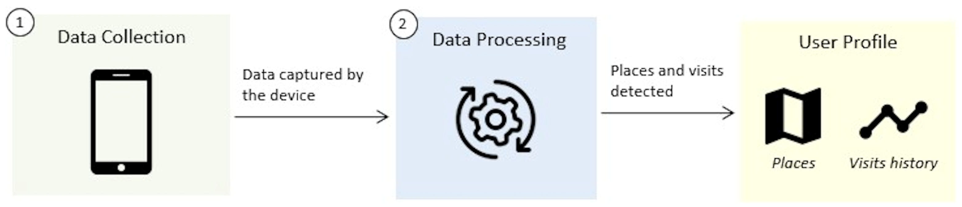
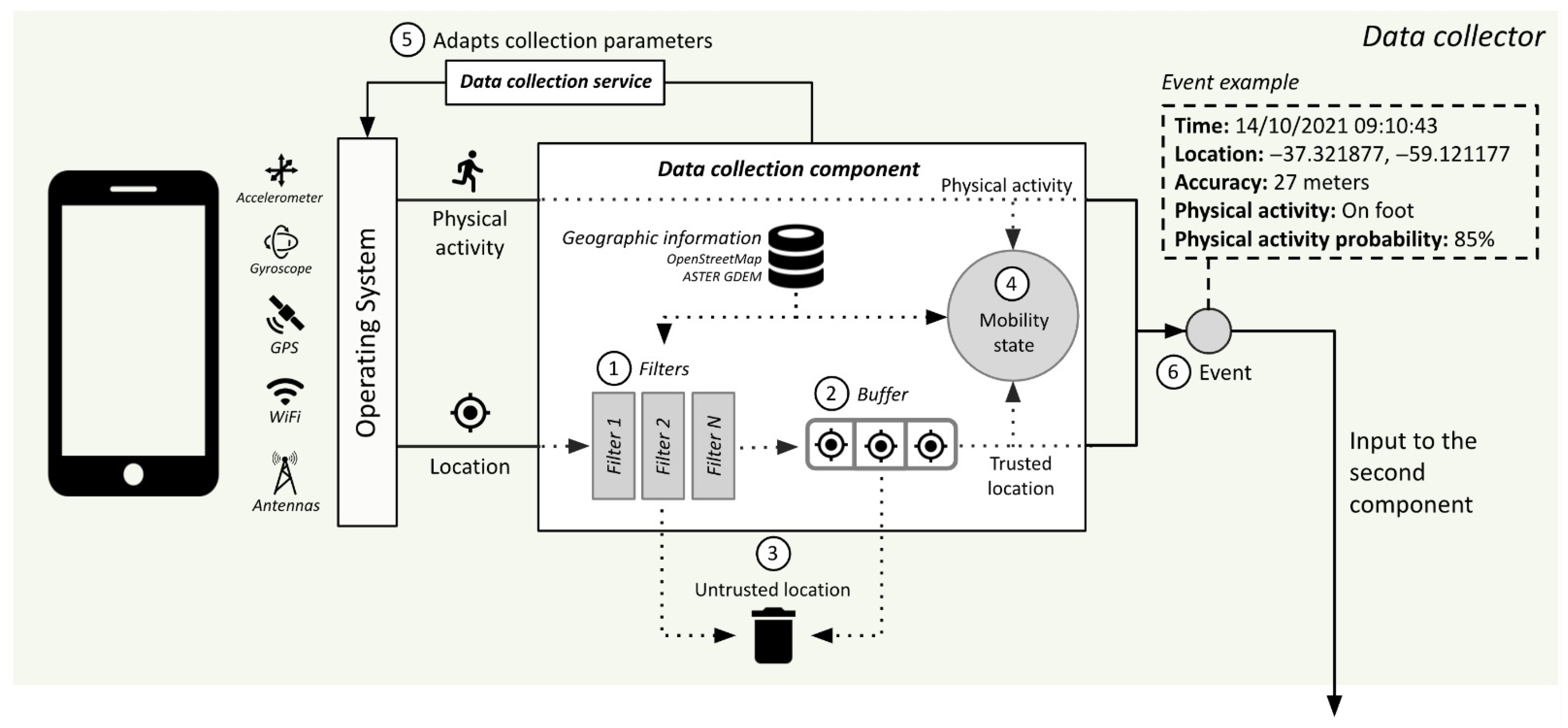
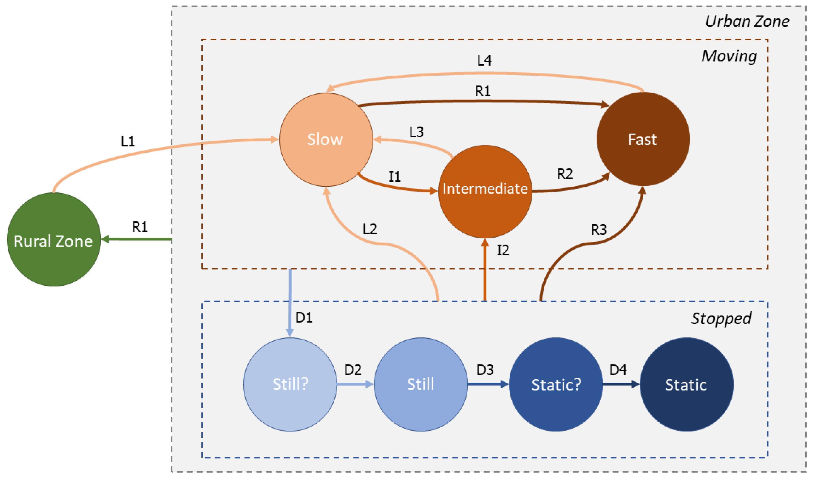
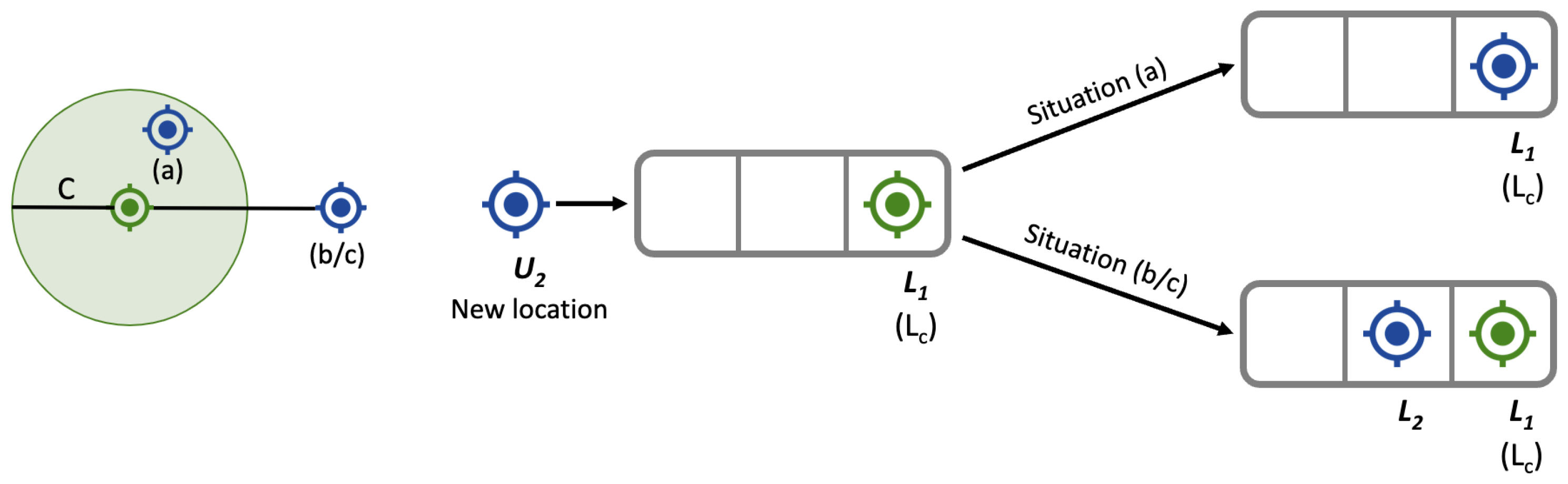
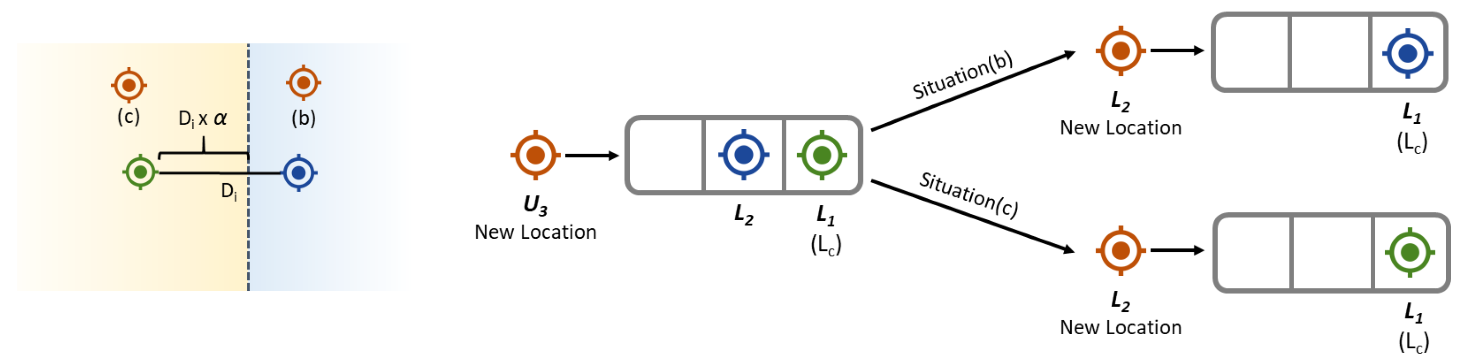
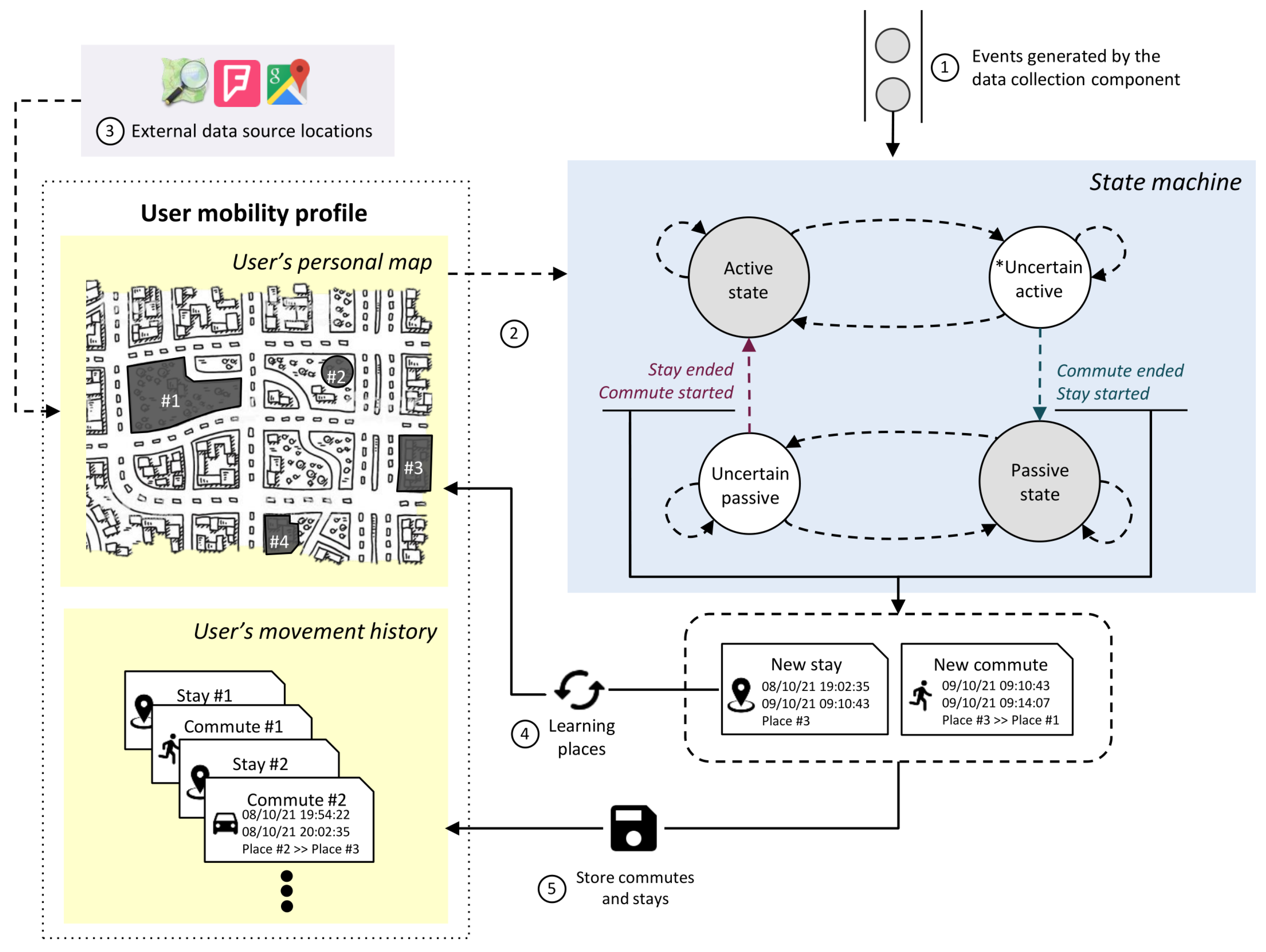
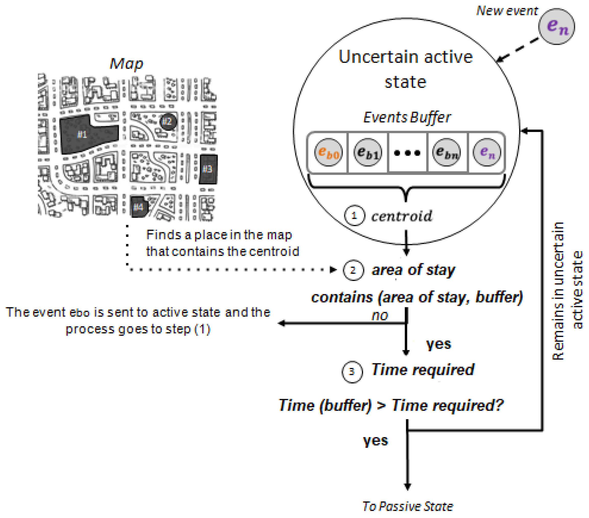
Table 1.
Mechanisms for estimating location.
| Source | Precision | Consumption | Comments |
|---|---|---|---|
| GSM | 400 m | 60 mW | It depends on antenna density [29] |
| Wi-Fi | 26 m | 90 mW | Unstable in outdoors [30] |
| GPS | 10 m | 400 mW | Unstable indoors [31] |
Table 2.
Data collection configuration according to the Mobility state.
| State | 1st Mechanism | Frequency | 2nd Mechanism | Frequency |
|---|---|---|---|---|
| Still? | WiFi | 40 seg | GPS | 80 seg |
| Still | WiFi | 2.5 min | GPS | 5 min |
| Static? | WiFi | 5 min | GPS | 10 min |
| Static | WiFi | 10 min | GPS | 20 min |
| Slow | WiFi | 40 seg | GPS | 80 seg |
| Intermediate | GPS | 15 seg | WiFi | 30 seg |
| Fast | GPS | 10 seg | WiFi | 20 seg |
Table 3.
Parameters to be tuned during the experiment.
| Parameter | Description | Values |
|---|---|---|
| p | Lower threshold of precision filter by precision (m) | 30|45|60 |
| P | Upper threshold of precision filter by precision (m) | | |
| C | Confidence threshold used in filter and buffer (m) | 15|30|45 |
| Threshold of high velocity for velocity filter (m/s) | 30|35|40 | |
| Threshold of intermediate velocity for velocity filter (Km/h) | 9|12|15 | |
| Threshold of low velocity for velocity filter (Km/h) | ||
| Memory time for errors for velocity filter (min) | 10|20|30 | |
| Altitude threshold for GPS filter by altitude (m) | 125|150|175 | |
| D | Filtering distance for outdoor network filter (m) | 10|20|30 |
| Location of the perpendicular in the buffer | 0.25|0.50|0.75 |
Table 4.
Results of the parameters’ tuning experiment.
| Configuration | Precision | Recall | F-Measure |
|---|---|---|---|
| 45-135-30-40-15-7-10-125-20-0.75 | 0.983942 | 0.962880 | 0.979656 |
| 45-135-30-35-15-7-10-125-30-0.75 | 0.983942 | 0.962880 | 0.979656 |
| 45-135-30-40-15-7-10-125-30-0.75 | 0.983942 | 0.962880 | 0.979656 |
| 45-135-30-35-15-7-10-125-20-0.75 | 0.983942 | 0.962880 | 0.979656 |
| 45-135-30-35-15-7-10-125-10-0.75 | 0.983938 | 0.962888 | 0.979655 |
| 45-135-30-40-15-7-10-125-10-0.75 | 0.983938 | 0.962888 | 0.979655 |
| 45-135-30-35-15-7-10-150-20-0.75 | 0.983933 | 0.962880 | 0.979649 |
| 45-135-30-35-15-7-10-175-30-0.75 | 0.983933 | 0.962880 | 0.979649 |
| 45-135-30-35-15-7-10-175-20-0.75 | 0.983933 | 0.962880 | 0.979649 |
| 45-135-30-40-15-7-10-150-30-0.75 | 0.983933 | 0.962880 | 0.979649 |
| 30-60-15-30-9-3-30-150-30-0.25 | 0.992473 | 0.876917 | 0.966988 |
| 60-120-15-30-9-3-30-150-10-0.25 | 0.986899 | 0.894749 | 0.966981 |
| 60-120-15-30-9-3-30-175-10-0.25 | 0.986899 | 0.894749 | 0.966981 |
| 60-120-15-30-9-3-30-175-30-0.25 | 0.986899 | 0.894734 | 0.966977 |
| 60-120-15-30-9-3-30-150-30-0.25 | 0.986899 | 0.894734 | 0.966977 |
| 60-120-15-30-9-3-30-125-30-0.25 | 0.986895 | 0.894720 | 0.966971 |
| 60-120-15-30-9-3-30-150-20-0.25 | 0.986895 | 0.894705 | 0.966968 |
| 60-120-15-30-9-3-30-175-20-0.25 | 0.986877 | 0.894741 | 0.966963 |
| 60-120-15-30-9-3-30-125-20-0.25 | 0.986877 | 0.894741 | 0.966963 |
| 60-120-15-30-9-3-30-150-30-0.25 | 0.986874 | 0.894712 | 0.966953 |
Table 5.
Results of the second stage experiments (whole dataset).
| Configuration | Precision | Recall | F-Measure |
|---|---|---|---|
| 45-135-30-40-15-7-20-125-30-0.75 | 0.989338 | 0.968880 | 0.985178 |
| 45-135-30-35-15-7-20-125-30-0.75 | 0.989338 | 0.96868 | 0.985175 |
| 45-135-30-40-15-7-20-125-20-0.75 | 0.989313 | 0.968954 | 0.985173 |
| 45-135-30-35-15-7-20-125-20-0.75 | 0.989313 | 0.968942 | 0.985171 |
| 45-135-30-40-15-7-20-125-30-0.5 | 0.989442 | 0.968423 | 0.985165 |
| 45-135-30-40-15-5-10-175-30-0.25 | 0.989351 | 0.966337 | 0.984661 |
| 45-135-30-35-15-5-10-125-10-0.25 | 0.989277 | 0.966590 | 0.984655 |
| 45-135-30-35-15-5-10-150-10-0.25 | 0.989256 | 0.966593 | 0.984639 |
| 45-135-30-35-15-5-10-175-10-0.25 | 0.989249 | 0.966604 | 0.984635 |
| 45-135-30-40-15-5-10-175-10-0.25 | 0.989246 | 0.966611 | 0.984635 |
| Original data | 0.357226 | 1.0 | 0.409924 |
Table 6.
Ablation study results for stay detection.
| Approach | Precision | Recall | F-Measure |
|---|---|---|---|
| Complete | 0.908 | 0.842 | 0.874 |
| Without Map | 0.878 | 0.836 | 0.856 |
| Normal Centroid | 0.878 | 0.821 | 0.849 |
| Fixed Area | 0.788 | 0.807 | 0.797 |
Table 7.
Ablation study results for place detection.
| Approach | Precision | Recall | F-Measure |
|---|---|---|---|
| Complete | 0.691 | 0.677 | 0.684 |
| Without Map | 0.656 | 0.681 | 0.668 |
| Normal Centroid | 0.672 | 0.673 | 0.673 |
| Fixed Area | 0.641 | 0.681 | 0.660 |
Table 8.
Best configurations for works in the literature for place detection.
| Related Work | Parameters | Precision | Recall | F-Measure |
|---|---|---|---|---|
| [48] | = 60 m | 0.7291 | 0.6362 | 0.6795 |
| [47] | = 60 m | 0.7339 | 0.6254 | 0.6753 |
| [31] | = 60 m | 0.7022 | 0.6337 | 0.6682 |
| [53] | = 37.5 m | 0.7215 | 0.6006 | 0.6555 |
Table 9.
Best configurations for works in the literature for stay detection.
| Related Work | Parameters | Precision | Recall | F-Measure |
|---|---|---|---|---|
| [47] | = 60, = 2 min | 0.8556 | 0.8115 | 0.8334 |
| [48] | = 60, = 2 min | 0.8400 | 0.8115 | 0.8255 |
| [31] | = 60, = 2 min | 0.8392 | 0.8117 | 0.8252 |
| [53] | = 60, = 2 min | 0.7080 | 0.6884 | 0.6981 |
Disclaimer/Publisher’s Note: The statements, opinions and data contained in all publications are solely those of the individual author(s) and contributor(s) and not of MDPI and/or the editor(s). MDPI and/or the editor(s) disclaim responsibility for any injury to people or property resulting from any ideas, methods, instructions or products referred to in the content. |
© 2023 by the authors. Licensee MDPI, Basel, Switzerland. This article is an open access article distributed under the terms and conditions of the Creative Commons Attribution (CC BY) license (https://creativecommons.org/licenses/by/4.0/).
Share and Cite
MDPI and ACS Style
Vallejos, S.; Berdun, L.; Armentano, M.; Schiaffino, S.; Godoy, D. A Lightweight Approach for Building User Mobility Profiles. ISPRS Int. J. Geo-Inf. 2024, 13, 11. https://doi.org/10.3390/ijgi13010011
AMA Style
Vallejos S, Berdun L, Armentano M, Schiaffino S, Godoy D. A Lightweight Approach for Building User Mobility Profiles. ISPRS International Journal of Geo-Information. 2024; 13(1):11. https://doi.org/10.3390/ijgi13010011
Chicago/Turabian StyleVallejos, Sebastián, Luis Berdun, Marcelo Armentano, Silvia Schiaffino, and Daniela Godoy. 2024. "A Lightweight Approach for Building User Mobility Profiles" ISPRS International Journal of Geo-Information 13, no. 1: 11. https://doi.org/10.3390/ijgi13010011
Note that from the first issue of 2016, this journal uses article numbers instead of page numbers. See further details here.