
Research on Traffic Accident Risk Prediction Method Based on Spatial and Visual Semantics
College of Resource and Environmental Engineering, Wuhan University of Science and Technology, Wuhan 430081, China
*
Author to whom correspondence should be addressed.
ISPRS Int. J. Geo-Inf. 2023, 12(12), 496; https://doi.org/10.3390/ijgi12120496
Submission received: 10 September 2023
/
Revised: 28 November 2023
/
Accepted: 4 December 2023
/
Published: 11 December 2023
Abstract
:Predicting traffic accidents involves analyzing historical data, determining the relevant factors affecting the occurrence of traffic accidents, and predicting the likelihood of future traffic accidents. Most of the previous studies used statistical methods or single deep learning network model prediction methods while ignoring the visual effects of the city landscape on the drivers and the zero-inflation problem, resulting in poor prediction performance. Therefore, this paper constructs a city traffic accident risk prediction model that incorporates spatial and visual effects on drivers. The improved STGCN model is used in the model, a CNN and GRU replace the origin space–time convolution layer, two layers of a GCN are added to extract the city landscape similarity of different regions, and a BN layer is added to solve the gradient explosion problem. Finally, the features extracted from the time–space correlation module, the city landscape similarity module and the spatial correlation module are fused. The model is trained with the self-made Chicago dataset and compared with the existing network model. The comparison experiment proves that the prediction effect of the model in both the full time period and the high-frequency time period is better than that of the existing model. The ablation experiment proves that the city landscape similarity module added in this paper performs well in the high-frequency area.
1. Introduction
With ongoing urbanization, the global motor vehicle count continues to rise annually. Urban growth has resulted in challenges like congestion, air pollution, noise, and traffic accidents on city roads. The most severe issue among these is traffic accidents. The 2022 Global Road Safety Report from the World Health Organization estimates around 2 million annual deaths due to diverse traffic accidents. Advances in data acquisition and computer hardware have led scholars to utilize traffic big data and deep learning for real-time traffic flow prediction, which can enable people to choose appropriate travel routes according to the prediction results to avoid traffic congestion. Integrating big data and deep learning offers a potential solution to predict and mitigate traffic accident risks.
An essential step in preventing traffic accidents is developing a predictive model that accurately assesses the risk in advance and notifies drivers to minimize accident risks. However, there are many factors that affect the occurrence of traffic accidents, so it is very difficult to accurately predict the risk of traffic accidents. For example, adverse weather conditions, road environment, and traffic flow can all have an impact on the occurrence of traffic accidents. In addition, the incidence of traffic accidents is also related to time, and the incidence of traffic accidents varies at different time periods. Therefore, effectively and dynamically predicting traffic accident risks remains a challenging issue.
Taking the Chicago area as an example, this study explores the accident risk of traffic accident occurrence areas from the perspectives of space, vision, and influencing factors. We also use deep learning methods to construct a traffic accident risk prediction model based on spatial and visual semantics, which is used to identify vulnerable areas in the neighborhood ranges of each region in the study area. It is expected that this research will provide technical support for urban planning and road design and provide a research paradigm for other studies.
2. Related Work
2.1. Deep Learning in Predicting Traffic Accidents’ Risk
Scholars have employed deep learning models to predict traffic and identify high-risk areas [1,2,3,4,5]. Numerous studies confirm the effectiveness of convolutional neural networks (CNNs) and recurrent neural networks (RNNs) in capturing spatial [6,7] and temporal [8,9] features. Chen et al. introduced the first city-level traffic accident prediction using a stacked denoising autoencoder (SDAE) [10]. Chen et al. extended their work, proposing a stacked denoising convolutional autoencoder (SDCAE) incorporating CNNs to model spatial dependencies in neighboring areas [11]. Yu et al. developed a deep spatiotemporal convolutional network to explore the relationship between traffic accidents and factors in Beijing [12]. Yuan et al. introduced the Hetero-ConvLSTM model, combining a CNN and RNN to model spatial environment heterogeneity [13]. Due to the strong spatial–temporal correlation in traffic data [14], data correlation can be represented as a characteristic graph, abstracting traffic accident prediction into graph data prediction. The graph convolution network, a deep learning model processing graph data, has broad applications, particularly in non-European data [15,16,17,18]. Scholars globally utilize space–time map convolution networks for studying traffic accident risk prediction. Zhou et al. introduced a differential spatiotemporal graph convolutional model, utilizing a dynamic graph based on static road features and dynamic traffic features to predict traffic flow and accident risks concurrently through multitask learning [19]. Guo et al. suggested a spatiotemporal attention graph convolutional model capturing traffic flow features in both time and space dimensions [20]. Wu et al. presented the GraphWave network, utilizing dilated causal convolutions to extend temporal feature range and enhance the model’s aggregation ability [21]. These studies improved model structures, allowing for a more comprehensive consideration of factors influencing traffic accidents. However, these studies did not consider the impact of visual feedback from the driving environment on driver behavior when selecting indicators.
2.2. Street View
Urban street scenes partially reflect a city’s spatial environment, revealing elements like vegetation, sky, buildings, roads, and vehicles. Accelerated urban construction results in urban roads with improved linearity, lower design speeds, and more complex visual environments. Hence, the driver’s perception and feedback can significantly impact the city’s traffic safety [22,23,24,25,26,27,28,29]. Presently, major map service providers offer a sufficient range of streetscape images covering city streets and alleys. As streetscape data availability improves and analysis methods mature, scholars increasingly use in-depth learning and streetscape images to study urban environments from a human perspective [30,31,32,33,34,35]. Mooney et al. analyzed Google Street View data (2007–2011), assessing nine features of 532 New York intersections to estimate the relationship between features and collision frequency [36]. The study found that infrastructure such as traffic islands, visual advertisements, bus stops, and pedestrian crosswalks were associated with an increase in pedestrian injuries in New York City. Zhang et al. used street view images to uncover spatiotemporal patterns of urban mobility from a resident’s perspective, demonstrating the images as a bridge connecting physical and human space. The study trained deep convolutional neural networks to recognize advanced scene features in street view images, explaining up to 66.5% of the hourly variation in taxi trips. The study demonstrated that inferring human activity at a fine-grained scale in urban areas through street imagery offers opportunities for environmental observation and intelligent city planning [24]. Urban driving involves a dynamic information interaction system with four factors: people, vehicles, roads, and the environment. Changes in roads, vehicles, and the driving environment transmit information to the driver. The research above offers the theoretical basis and methods for this paper to use street view images for simulating driver visual changes, proving that alterations in the traffic environment lead to traffic accidents [37,38]. Thus, when addressing traffic accident risk prediction, the impact of the traffic environment on drivers must be considered.
In this paper, we propose a novel model capturing simultaneous spatial–temporal correlations and visual semantics, expected to enhance traffic accident risk forecasting performance.
3. Preliminaries
Definition 1.
Region. A city is divided into grids based on the longitude and latitude, where a grid represents a region and all regions have the same size. Note that city shapes are typically irregular, resulting in regions with road segments. In these N regions, we can collect their actual features and traffic accident points, while in other regions, we set zero values for their features.
Definition 2.
Traffic Accident Type. According to the number of casualties in traffic accidents, we define three traffic accident types, i.e., minor accidents, injured accidents and fatal accidents, and corresponding risk values are set to be 1, 2 and 3, respectively.
Problem statement: Traffic Accident Forecasting. Let represent the grid features of all the regions at time interval t, including the information of weather, POI, traffic flow and traffic accident risk, where is the dimension of region features. Let denote the signal matrix of the three graphs at time interval t. Each row represents a node’s features, including the values of traffic flow and traffic accident risk, where dg is the dimension of node features. Let be the time information of time interval t, including hour of day, day of week and if it is a holiday, where dt is the dimension of time features. Given the historical observations of region features , graphs signal matrices and , our goal is to predict the traffic accident risk at the next time interval, i.e., .
4. Spatial and Visual Semantics Network
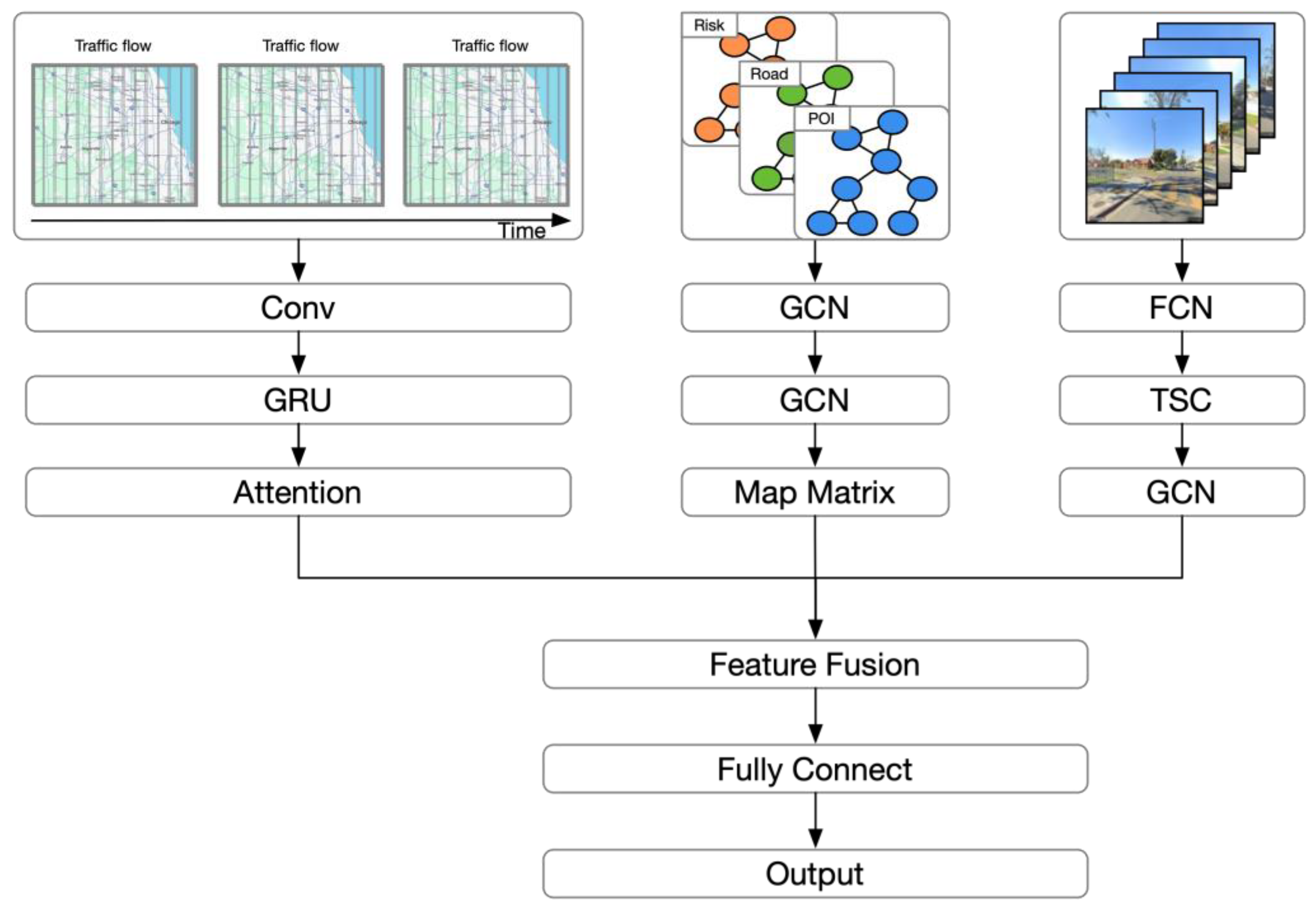
The paper introduces SVSNet, a traffic accident risk prediction model illustrated in Figure 1, comprising three key components: spatiotemporal correlation module, spatial correlation module, and visual semantic feature extraction module. The spatiotemporal correlation module, utilizing grid features and time data, initially models the spatial correlation with CNN, captures time dependencies with GRU, and dynamically adjusts historical information importance using an attention mechanism for prediction. The image feature extraction module processes street view images and road similarity maps as input, computes traffic scene complexity through semantic segmentation, and integrates the road similarity map with GCN to derive street view similarity features among regions. The spatial correlation module extracts spatial features by aggregating neighboring node features with two layers of GCN. The feature fusion prediction module weights and combines outputs from the initial three modules to generate the prediction value. The network structure diagram is shown in Figure 1.
4.1. Training and Testing Data
The study area selected for the experiment is Chicago, and the prediction scope is divided into 2 km × 2 km square grids based on geographical location. The study employs Chicago data summarized in Table 1, encompassing seven types: traffic accidents, taxi orders, POI, weather, road, and building data.
The traffic accident data include the time of occurrence, number of casualties, and the longitude and latitude of the accident location; the taxi order data include the pick-up and drop-off times and the longitude and latitude; the road data include the road grade, length, location, and other attributes; the weather data include the temperature and weather conditions; and the POI data include nine categories: catering, shopping, entertainment, living facilities, sports facilities, cultural facilities, educational facilities, medical facilities, and scenic spots.
4.2. Data Processing
4.2.1. Traffic Accidents Data
Traffic accidents are categorized as mild, moderate, or severe based on injury and damage. The corresponding risk levels are 1, 2, and 3. Traffic accidents are then matched with corresponding areas and times based on their time and location. The total accident risk is calculated by summing the risks of all traffic accidents in that area for the specified time period.
4.2.2. Taxi Order Data
Passenger pick-up and drop-off data, like traffic accident data, are matched to the corresponding area and time period using longitude, latitude, and timestamp. The outflow and inflow of taxis during the specified time period are calculated. Outflow denotes vehicles leaving the area (pick-up within, drop-off outside), and inflow is the reverse. We use taxi orders to simulate the traffic flow.
4.2.3. Points of Interest
The article categorizes POI (point of interest) data into nine types: dining, shopping, entertainment, daily facilities, sports facilities, cultural facilities, educational facilities, medical facilities, and scenic spots. Each POI category is matched to the area using its latitude and longitude, and a nine-dimensional vector is formed by calculating the number of each POI type in that area. For instance, if a gym is present in the area, the feature vector would be (0, 0, 0, 0, 1, 0, 0, 0, 0).
4.2.4. Road Data
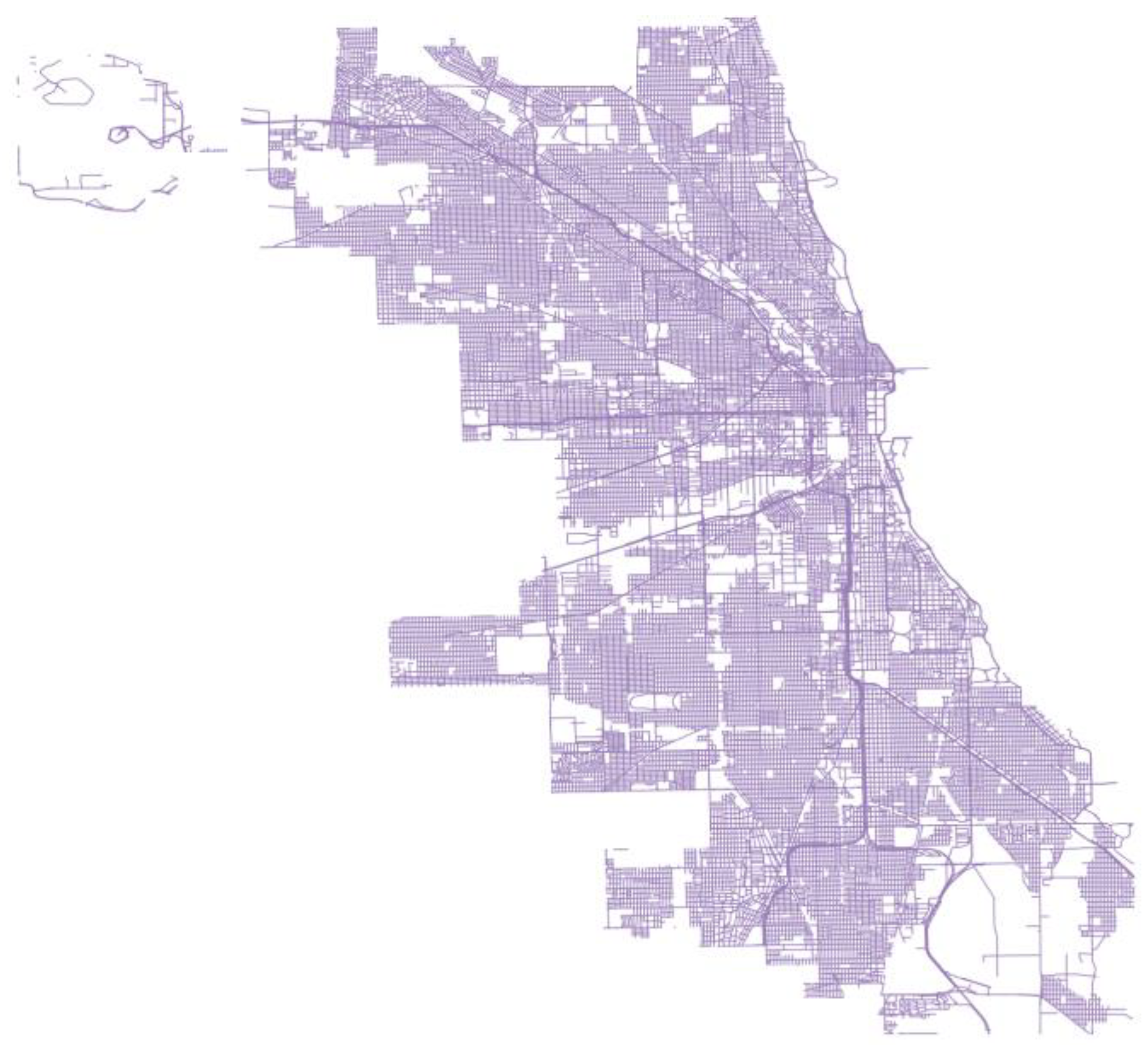
The road data are collected from OSM. The road data contain road attribute data and road geometry data, as shown in Figure 2 and Table 2.
Road geometric data can be extracted from the shapefile data, as shown in Figure 2. Road features, including the number of intersections, road grade, and road length, were collected from the road geometry data.
By matching the latitude and longitude of roads to their respective regions, we calculated the total length, number of intersections, and road types for each region. The road similarity for each region was determined using JS divergence, which is expressed by the following formula:
where and represent the road characteristics of areas i and j; represents the similarity degree of road characteristics between region i and j, and the value range is between [0, 1].
4.2.5. Weather Data
The weather data include hourly temperature and weather conditions. Temperature is presented as a continuous value, while weather conditions are categorized into five classes: sunny, rainy, snowy, cloudy, and foggy, which are represented as one-hot vectors. For instance, if the current temperature is 5 °C and the weather is sunny, the corresponding weather feature vector is (5, 1, 0, 0, 0, 0).
4.2.6. Street View Image
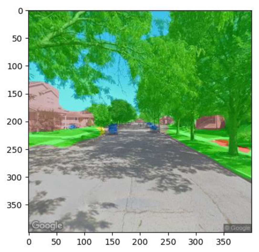
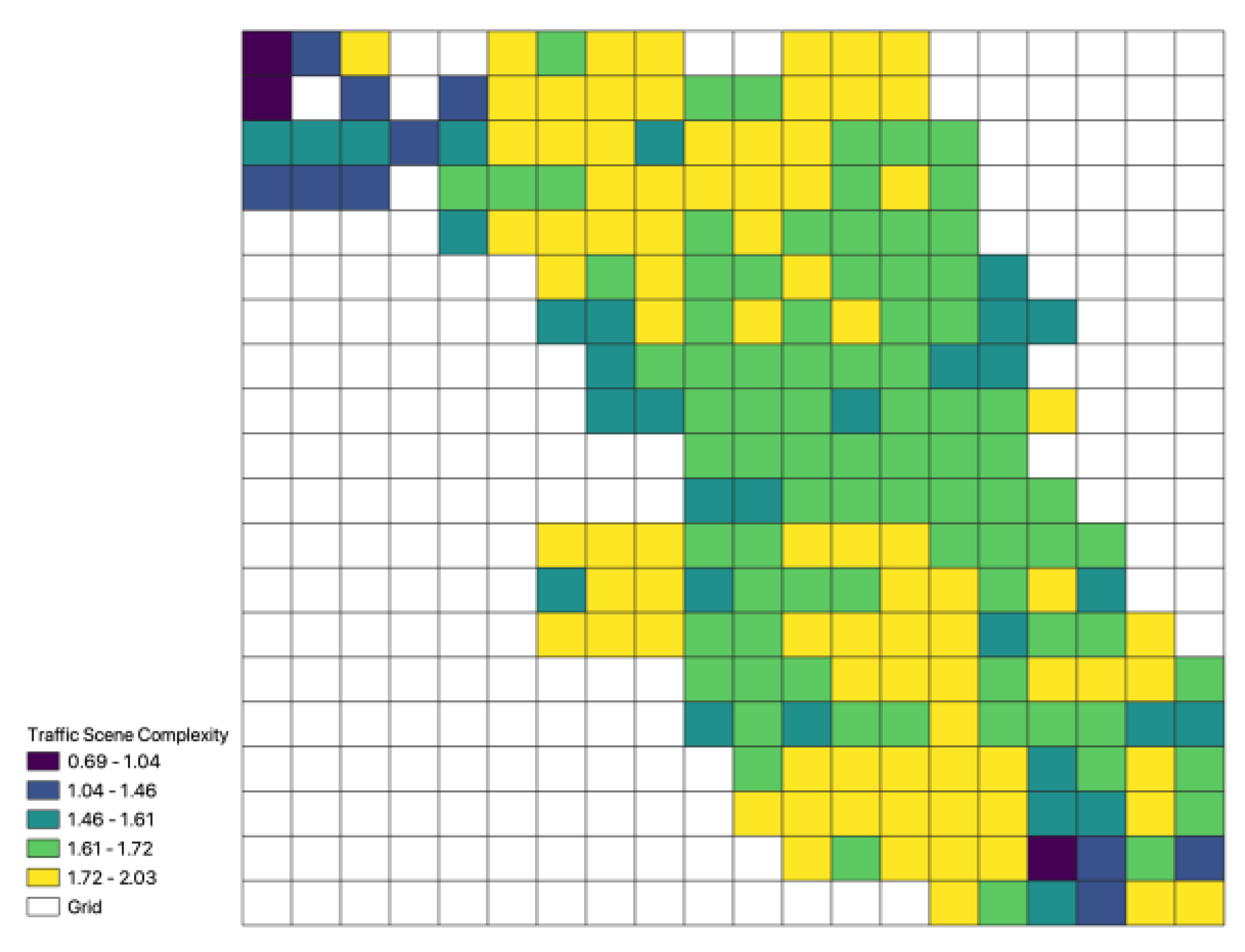
The study employs street view images to simulate the driver’s perception of the urban landscape, recognizing that higher driving environment complexity correlates with increased accident likelihood. Street view images are utilized for calculating traffic scene complexity, employing semantic segmentation to identify objects in the driver’s field of view. Proportions of object categories in the field of view are calculated based on semantic segmentation results. The complexity of individual traffic scenes (roads) is then computed using an improved gravity model [39], and the overall traffic scene complexity in the study area is derived by summing up complexities across all traffic scenes.
Using the ADE20K dataset, a model is trained with Deeplab-v3 network as the backbone for the semantic segmentation of street view images [40,41]. The segmentation results are shown in Figure 3.
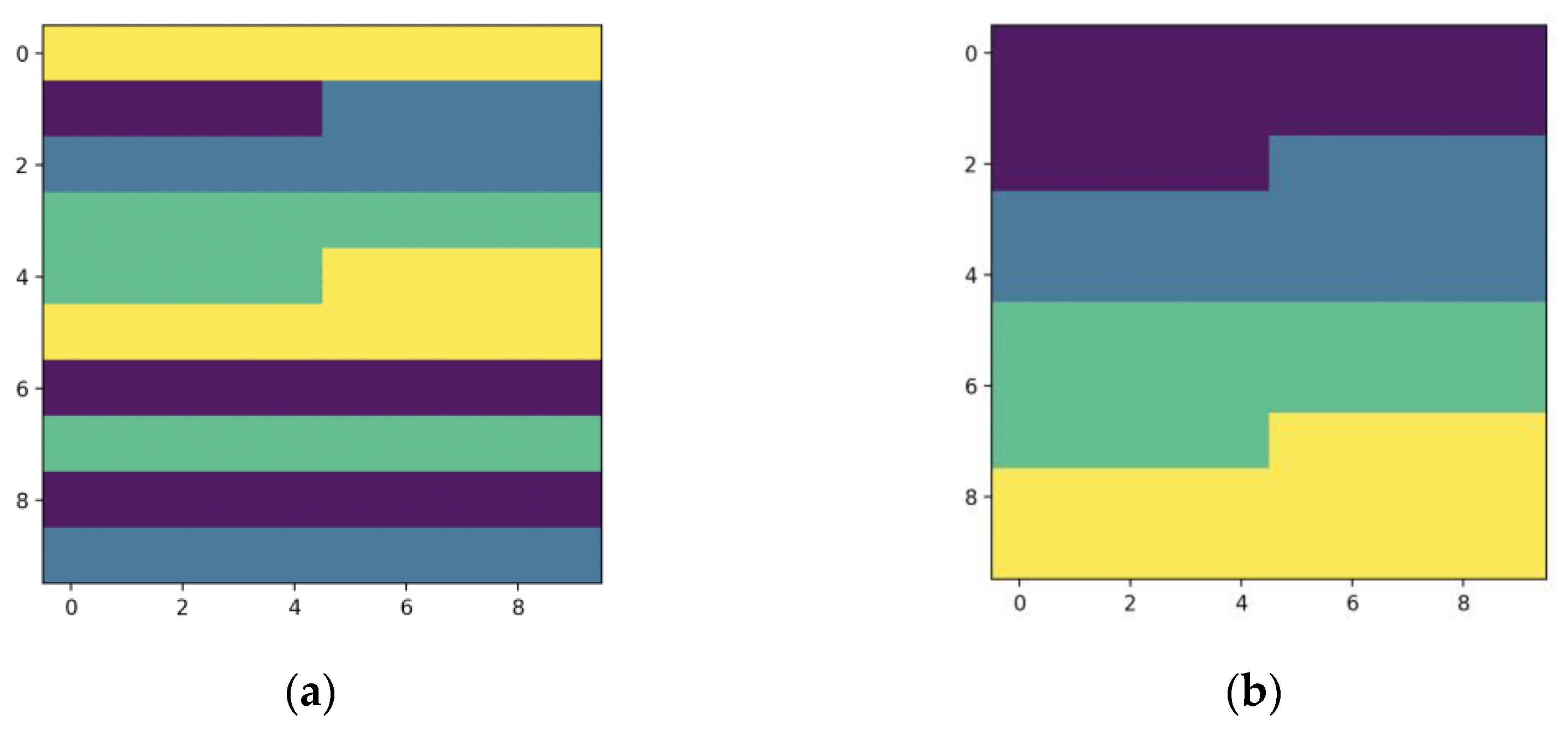
Considering the influence of road environments on drivers is crucial for predicting traffic accident risks, but existing methods often analyze the statistical proportions of influential objects across the entire field of view. However, this approach neglects the spatial distribution of these objects, making it challenging to accurately capture the complexity of traffic scenes, as illustrated in Figure 4.
Figure 4 displays images with an equal number of pixels for each class, where the traditional calculation method only considers pixel category and proportion. Consequently, the upper figures have the same calculated complexity. However, it is evident from the figure that the distribution in (a) is more disorderly, significantly impacting the driver’s line of sight. Therefore, solely considering pixel proportions fails to accurately describe traffic scene complexity.
Therefore, this paper proposes a traffic scene complexity calculation model based on the gravity model. By introducing an information entropy model into the gravity model, a mathematical model for describing the complexity of a single traffic scene is constructed, as shown in Equations (3)–(5):
represents the label of each pixel after segmentation; N represents the width and height of the image (the street view images collected in this paper have a size of , so is used to represent the image size); represents the relative velocity between the driver and the object, since the study focuses on urban roads and mainly considers static objects, the speed limit of the road is used as a proxy for relative velocity; represents the complexity of the scene; S represents the visual distance between the driver and the object, and the average distance of the line of sight is used as the visual distance in this paper.
Using the model designed in this paper for calculation, the complexity of (a) and (b) are 2.118659262428785 and 2.0527425251086986, respectively, showing significant differences. The traffic scene complexity of the study area is shown in Figure 5.
4.3. Model Construction and Train Parameters
4.3.1. Spatial Correlation Module
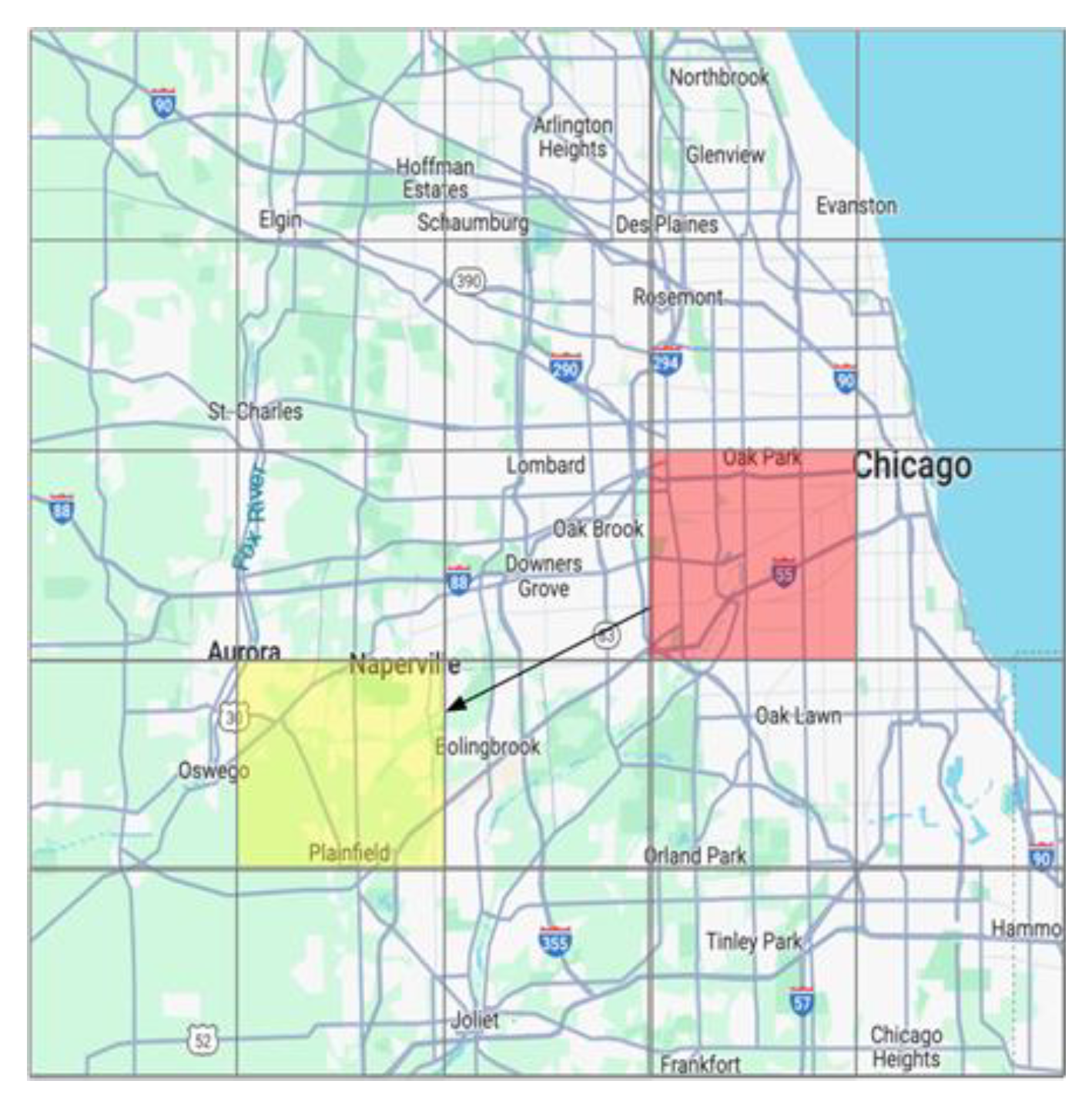
The spatial correlation of traffic accidents often exists in a local area. For example, if there is traffic congestion in a neighboring area, it may affect the occurrence of traffic accidents in the target area, as shown in Figure 6.
Due to the connectivity of the road network, neighboring traffic scenes may also have some similarity. To capture the spatial correlation within a local area, a two-layer graph convolutional network (GCN) is used, with the GCN layers shared across the temporal dimension. The two-layer GCN can aggregate values that are two units away from the target area and thus obtain the features that are two units away from the target area. The specific operations are as follows:
where W and b are learnable parameters; A is the graph signal matrix; S′ is the result of two-level graph convolution output.
4.3.2. Space–Time Correlation Module
The module utilizes a CNN to model the spatial correlation, employs a GRU to capture temporal similarity, and incorporates an attention mechanism for dynamic weight capture in the time dimension. Traffic accidents exhibit similarities in both time and space; the CNN captures the spatial similarity shared across the time dimension. The data at each time step are convolved using the formula when processing the input at each time step:
where is the activation function; is a learnable parameter; and X is the characteristic vector.
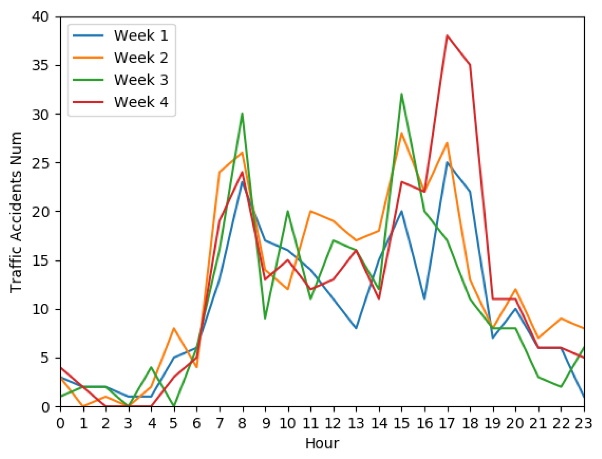
The GRU captures both long-term and short-term features of traffic accidents in the time dimension, considering how past traffic conditions may influence accidents at the target time. Additionally, traffic accidents exhibit global features, as illustrated in Figure 7, depicting the weekly periodicity of accidents on Tuesdays for four consecutive weeks in the global area.
To capture the long-term and short-term features in the temporal dimension, the first p time periods of the target period and the data of the target grid for the previous q weeks are selected as the training data . The GRU module is used as the temporal feature-capturing module. The GRU calculation process of the defined area i in the time step t is as follows:
where is the output result of the local space convolution of the region time step t. represent the reset gate and the update gate, respectively, and are candidate hidden states and hidden states. and are weight parameters, is the deviation parameter, and is the number of hidden cells in the GRU. A is the sigmoid function, which transforms the value of the element to [0, 1], is the Tanh function. is Hadamaji. , where represents the hidden state of all regions in time step t.
Finally, the SoftMax function is used to weight the prediction results of different historical times. All predicted values of the historical segments are weighted and summed to obtain the output of the spatiotemporal correlation module. The specific formula is as follows:
where W and b are learnable parameters; H represents the hidden state in different time periods; represents the time information of the target time; α represents the score (weight); and Y represents the output.
4.3.3. Visual Semantic Feature Module
Utilizing the Deeplab-v3 network, the module segments street view images and calculates the complexity of a single traffic scene using the proposed formula. The area’s traffic scene complexity is determined accordingly. Visual semantic features of the target area are obtained by weighing the traffic scene complexity and road similarity. Subsequently, a two-layer GCN network is employed to establish visual semantic similarity between different regions, as detailed in Equations (3)–(6).
5. Estimation Performance of the Model
5.1. Experimental Environment and Parameter Configuration
The experimental configuration of this article is shown in Table 3:
Implementing a bimodal model in the PyTorch framework, we partition the training, validation, and testing sets in a chronological order of 6:2:2. Following experimental comparisons and a literature review, the hyperparameters are determined: the adjacent time period is set as p = 3; the GRU comprises 3 layers, each with 128 hidden units; the GCN consists of 2 layers with a kernel size of 16; the CNN employs a kernel size of 3 × 3; the batch size is 8; the learning rate is 1 × 10⁻⁶; and early stopping is employed to prevent overfitting.
5.2. Evaluation Metrics and Loss Function
In order to make the evaluation results more comprehensive, the evaluation indicators selected in this paper are the root mean square error (RMSE), classification index recall rate (Recall) and mean absolute error (MAE). The specific calculation formula is as follows:
where represents the actual accident risk for all regions at time t; represents the predicted accident risk for all regions at time t; represents the set of regions where traffic accidents actually occurred at time t; represents the set of regions in the top predicted accident risk ranking; represents the accuracy sorting list from 1 to j; represents whether a traffic accident occurred, where means a traffic accident occurred at time t, and means no traffic accident occurred at time t.
A higher RMSE indicates that the model predicts accident risks more accurately across all areas. A higher recall and MAP indicate that the model predicts high-risk areas better: that is, the model is more likely to discover high-risk areas.
Since the area where traffic accidents occur in the real dataset is far smaller than the area where there are no traffic accidents, there are a lot of zero values in the tag, leading to the zero-inflated model problem. In order to solve the zero-inflated model problem, the weighted mean square loss function is used in this paper. When calculating the loss, a larger weight value is given to the area with traffic accidents so as to avoid the predicted value near 0. The calculation formula is as follows:
where represents the actual accident risk; represents the predicted accident risk; and represents weighted value.
5.3. Experimental Results and Analysis
To evaluate the performance of the proposed SVSNet model, a comparison was made with benchmark and classical models. The models used in this experiment include the Historical Average (HA) model, Multi-Layer Perceptron (MLP) model, Gated Recurrent Unit (GRU) model, Convolutional Neural Network (CNN)-based Stacked Denoising Autoencoder (SDACE) model, Heterogeneous Convolutional Long Short-Term Memory (Hetero-convLSTM) model combining CNN and LSTM, and a machine learning model based on Gradient Boosting Tree (XGBoost), in addition to the proposed SVSNet model.
The Table 4 presents the prediction performance of various models on the dataset. SVSNet consistently outperforms other methods across all time periods, demonstrating its superior ability to capture temporal, spatial, and image features. HA, XGBoost, GRU, and MLP exhibit poor performance, as they solely rely on historical data features and focus only on temporal correlation, neglecting spatial features. SDCAE captures spatial correlation but lacks consideration of temporal correlation. Hetero-ConvLSTM addresses both temporal and spatial correlation but overlooks the visual effects of the driver and the global data correlation. The proposed model, accounting for driver visual effects and spatiotemporal correlation, achieves superior prediction performance.
6. Discussion
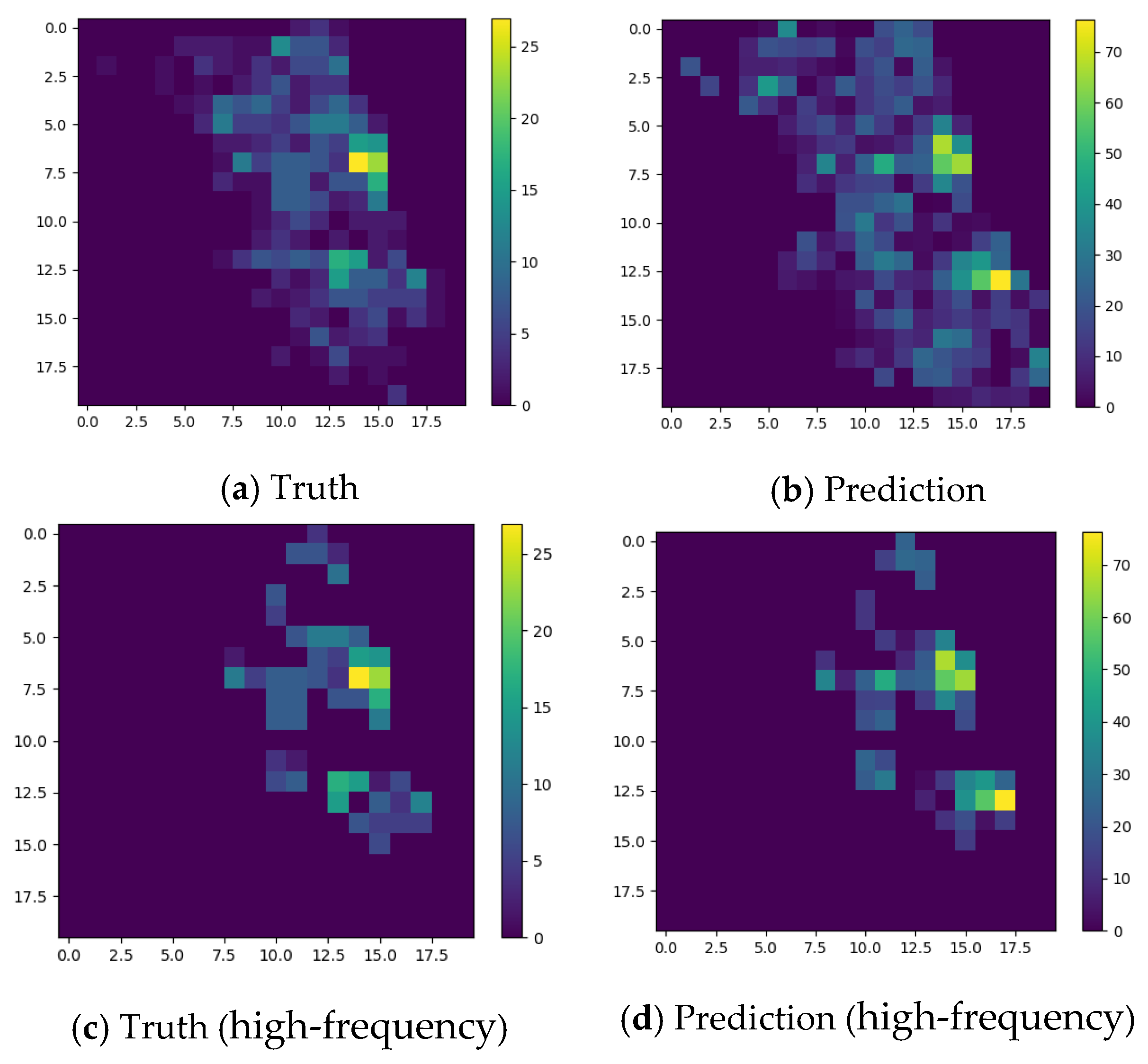
To assess our model’s ability to predict traffic accident risk, we visualize the results on the test set. Figure 7 displays the heatmap of predicted traffic accident risk and true labels in the study area for the entire and high-frequency time period (10 September to 17 September 2016). Observing Figure 8 reveals the close similarity between predicted and true values, affirming the model’s accuracy. Sparse traffic accident data are noted with high-risk regions limited. Notably, in city centers with high traffic flow, predicted heatmaps closely align with true values, emphasizing the model’s effectiveness in considering the driver’s visual effect.
The existing research results have demonstrated the superiority of CNN and GRU in mining spatiotemporal correlations between data, and they also demonstrated that spatiotemporal graph convolutional networks perform better than other models in the field of traffic accident risk prediction [42,43,44,45]. To further validate the effectiveness of the designed modules, this study conducted an ablation experiment to verify the effectiveness of the visual effect extraction module. The results of the test on the dataset are shown in Table 5:
Table 5 shows the results of ablation experiments conducted to further validate the effectiveness of the visual attention module. As shown, the model with the visual attention module performed better in terms of recall and MAP but not in terms of RMSE compared to the baseline model without this module. The main reason for this is that the study area was divided into a 20 × 20 grid, of which only 197 grids belonged to the study area. To facilitate model construction, the dataset size was set to (20, 20), so the predicted result size was also (20, 20), including 203 invalid data points. Among these 203 invalid predictions, there may be some outliers with very large deviation, which resulted in the increase in the RMSE value. However, when calculating recall and MAP, only high-risk area data were used, and there were no invalid data, resulting in better performance for these two indicators. This demonstrates the importance of modeling driver visual attention in traffic accident risk prediction.
7. Conclusions
In this study, we proposed a gravity model-based approach to assess traffic scene complexity and quantify its impact on drivers. Subsequently, a spatial and visual semantic-based traffic accident risk prediction model was developed, integrating CNN, GCN, GRU, and an attention mechanism to extract and merge spatial–temporal features and relationships from traffic accident data. Model validation utilized Chicago’s traffic accident data from January to December 2016, evaluating metrics like MAP, recall, and RMSE. The key findings follow.
Predictions align closely with observed results. Ablation experiments reveal improved model performance with the added visual semantics module. In full-time prediction, the model with this module outperforms in MAP and recall but has a slightly higher RMSE compared to the model without this module. In high-risk period prediction, all three indicators are superior. Overall, the model effectively forecasts the spatial–temporal distribution of traffic accidents.
The prediction method employs gridding in the study area, aiding government urban planning. Introducing a weighted loss function enhances model focus on accident-prone areas, improving predictive capability. However, there is room for model improvement. The construction of a grid to organize data covers both the study area and data-free regions. These blank areas may affect the model, warranting further discussion in future research to define the study area.
Author Contributions
Conceptualization, Wenjing Li and Zihao Luo; Methodology, Wenjing Li and Zihao Luo; Software, Wenjing Li and Zihao Luo; Validation, Wenjing Li and Zihao Luo; Formal analysis, Wenjing Li and Zihao Luo; Resources, Wenjing Li and Zihao Luo; Data curation, Wenjing Li and Zihao Luo; Writing, Wenjing Li and Zihao Luo; Supervision, Wenjing Li and Zihao Luo All authors have read and agreed to the published version of the manuscript.
Funding
This research received no external funding.
Institutional Review Board Statement
Not applicable.
Informed Consent Statement
Not applicable.
Data Availability Statement
Publicly available datasets were analyzed in this study. This data can be found here: [https://data.cityofchicago.org/].
Conflicts of Interest
The authors declare no conflict of interest.
Correction Statement
This article has been republished with a minor correction to the Data Availability Statement. This change does not affect the scientific content of the article.
References
- Ben-Akiva, M.; Bierlaire, M.; Koutsopoulos, H.; Mishalani, R. DynaMIT: A simulation-based system for traffic prediction. In Proceedings of the DACCORD Short Term Forecasting Workshop, Delft, The Netherlands, February 1998. [Google Scholar]
- Yin, X.; Wu, G.; Wei, J.; Shen, Y.; Qi, H.; Yin, B. Deep learning on traffic prediction: Methods, analysis, and future directions. IEEE Trans. Intell. Transp. Syst. 2021, 23, 4927–4943. [Google Scholar] [CrossRef]
- Yuan, H.; Li, G. A survey of traffic prediction: From spatio-temporal data to intelligent transportation. Data Sci. Eng. 2021, 6, 63–85. [Google Scholar] [CrossRef]
- Zheng, C.; Fan, X.; Wang, C.; Qi, J. Gman: A graph multi-attention network for traffic prediction. In Proceedings of the AAAI Conference on Artificial Intelligence, New York, NY, USA, 7–12 February 2020; pp. 1234–1241. [Google Scholar]
- Zhao, L.; Song, Y.; Zhang, C.; Liu, Y.; Wang, P.; Lin, T.; Deng, M.; Li, H. T-gcn: A temporal graph convolutional network for traffic prediction. IEEE Trans. Intell. Transp. Syst. 2019, 21, 3848–3858. [Google Scholar] [CrossRef]
- Sermanet, P.; Eigen, D.; Zhang, X.; Mathieu, M.; Fergus, R.; LeCun, Y. Overfeat: Integrated recognition, localization and detection using convolutional networks. arXiv 2013, arXiv:1312.6229. [Google Scholar]
- He, K.; Zhang, X.; Ren, S.; Sun, J. Deep residual learning for image recognition. In Proceedings of the IEEE Conference on Computer Vision and Pattern Recognition, Las Vegas, NV, USA, 27–30 June 2016; pp. 770–778. [Google Scholar]
- Li, S.; Li, W.; Cook, C.; Zhu, C.; Gao, Y. Independently recurrent neural network (indrnn): Building a longer and deeper rnn. In Proceedings of the IEEE Conference on Computer Vision and Pattern Recognition, Salt Lake City, UT, USA, 8–12 June 2018; pp. 5457–5466. [Google Scholar]
- Sherstinsky, A. Fundamentals of recurrent neural network (RNN) and long short-term memory (LSTM) network. Phys. D Nonlinear Phenom. 2020, 404, 132306. [Google Scholar] [CrossRef]
- Chen, Q.; Song, X.; Yamada, H.; Shibasaki, R. Learning deep representation from big and heterogeneous data for traffic accident inference. In Proceedings of the Thirtieth AAAI Conference on Artificial Intelligence, Phoenix, AZ, USA, 12–17 February 2016. [Google Scholar]
- Chen, C.; Fan, X.; Zheng, C.; Xiao, L.; Cheng, M.; Wang, C. Sdcae: Stack denoising convolutional autoencoder model for accident risk prediction via traffic big data. In Proceedings of the 2018 Sixth International Conference on Advanced Cloud and Big Data (CBD), Lanzhou, China, 12–15 August 2018; pp. 328–333. [Google Scholar]
- Yu, L.; Du, B.; Hu, X.; Sun, L.; Han, L.; Lv, W. Deep spatio-temporal graph convolutional network for traffic accident prediction. Neurocomputing 2021, 423, 135–147. [Google Scholar] [CrossRef]
- Yuan, Z.; Zhou, X.; Yang, T. Hetero-convlstm: A deep learning approach to traffic accident prediction on heterogeneous spatio-temporal data. In Proceedings of the Proceedings of the 24th ACM SIGKDD International Conference on Knowledge Discovery & Data Mining, London, UK, 19–23 August 2018; pp. 984–992. [Google Scholar]
- Huang, Y.; Shekhar, S.; Xiong, H. Discovering colocation patterns from spatial data sets: A general approach. IEEE Trans. Knowl. Data Eng. 2004, 16, 1472–1485. [Google Scholar] [CrossRef]
- Lei, K.; Qin, M.; Bai, B.; Zhang, G.; Yang, M. GCN-GAN: A non-linear temporal link prediction model for weighted dynamic networks. In Proceedings of the IEEE INFOCOM 2019-IEEE Conference on Computer Communications, Paris, France, 29 April–2 May 2019; pp. 388–396. [Google Scholar]
- Yan, M.; Deng, L.; Hu, X.; Liang, L.; Feng, Y.; Ye, X.; Zhang, Z.; Fan, D.; Xie, Y. Hygcn: A gcn accelerator with hybrid architecture. In Proceedings of the 2020 IEEE International Symposium on High Performance Computer Architecture (HPCA), San Diego, CA, USA, 22–26 February 2020; pp. 15–29. [Google Scholar]
- Yu, B.; Lee, Y.; Sohn, K. Forecasting road traffic speeds by considering area-wide spatio-temporal dependencies based on a graph convolutional neural network (GCN). Transp. Res. Part C Emerg. Technol. 2020, 114, 189–204. [Google Scholar] [CrossRef]
- Zhang, S.; Yin, H.; Chen, T.; Hung, Q.V.N.; Huang, Z.; Cui, L. Gcn-based user representation learning for unifying robust recommendation and fraudster detection. In Proceedings of the 43rd International ACM SIGIR Conference on Research and Development in Information Retrieval, Xi’an, China, 25–30 July 2020; pp. 689–698. [Google Scholar]
- Zhou, Z.; Wang, Y.; Xie, X.; Chen, L.; Liu, H. RiskOracle: A minute-level citywide traffic accident forecasting framework. In Proceedings of the AAAI Conference on Artificial Intelligence, New York, NY, USA, 7–12 February 2020; pp. 1258–1265. [Google Scholar]
- Guo, S.; Lin, Y.; Feng, N.; Song, C.; Wan, H. Attention based spatial-temporal graph convolutional networks for traffic flow forecasting. In Proceedings of the AAAI Conference on Artificial Intelligence, Honolulu, HI, USA, 27 January–1 February 2019; pp. 922–929. [Google Scholar]
- Wu, Z.; Pan, S.; Long, G.; Jiang, J.; Zhang, C. Graph wavenet for deep spatial-temporal graph modeling. arXiv 2019, arXiv:1906.00121. [Google Scholar]
- Colonna, P.; Berloco, N.; Intini, P.; Ranieri, V. Route familiarity in road safety: Speed choice and risk perception based on a on-road study. In Proceedings of the Transportation Research Board 94th Annual Meeting, Washington, DC, USA, 11–15 January 2015. [Google Scholar]
- Leng, H.; Lin, Y.; Zanzi, L. An experimental study on physiological parameters toward driver emotion recognition. In Proceedings of the Ergonomics and Health Aspects of Work with Computers: International Conference, EHAWC 2007, Held as Part of HCI International 2007, Beijing, China, 22–27 July 2007; pp. 237–246. [Google Scholar]
- Zhang, F.; Wu, L.; Zhu, D.; Liu, Y. Social sensing from street-level imagery: A case study in learning spatio-temporal urban mobility patterns. ISPRS J. Photogramm. Remote Sens. 2019, 153, 48–58. [Google Scholar] [CrossRef]
- Young, A.H.; Mackenzie, A.K.; Davies, R.L.; Crundall, D. Familiarity breeds contempt for the road ahead: The real-world effects of route repetition on visual attention in an expert driver. Transp. Res. Part F Traffic Psychol. Behav. 2018, 57, 4–9. [Google Scholar] [CrossRef]
- Zhang, T.; Sun, L.; Yao, L.; Rong, J. Impact analysis of land use on traffic congestion using real-time traffic and POI. J. Adv. Transp. 2017, 2017, 7164790. [Google Scholar] [CrossRef]
- Wolf, K.L.; Bratton, N. Urban trees and traffic safety: Considering US roadside policy and crash data. Arboric. Urban For. 2006, 32, 170. [Google Scholar] [CrossRef]
- Thiffault, P.; Bergeron, J. Monotony of road environment and driver fatigue: A simulator study. Accid. Anal. Prev. 2003, 35, 381–391. [Google Scholar] [CrossRef] [PubMed]
- Harbluk, J.L.; Noy, Y.I.; Trbovich, P.L.; Eizenman, M. An on-road assessment of cognitive distraction: Impacts on drivers’ visual behavior and braking performance. Accid. Anal. Prev. 2007, 39, 372–379. [Google Scholar] [CrossRef] [PubMed]
- Hu, S.; Gao, S.; Wu, L.; Xu, Y.; Zhang, Z.; Cui, H.; Gong, X. Urban function classification at road segment level using taxi trajectory data: A graph convolutional neural network approach. Comput. Environ. Urban Syst. 2021, 87, 101619. [Google Scholar] [CrossRef]
- Naik, N.; Philipoom, J.; Raskar, R.; Hidalgo, C. Streetscore-Predicting the Perceived Safety of One Million Streetscapes. In Proceedings of the 2014 IEEE Conference on Computer Vision and Pattern Recognition Workshops, Columbus, OH, USA, 23–28 June 2014; pp. 793–799. [Google Scholar]
- Zhou, H.; Liu, L.; Lan, M.; Zhu, W.; Song, G.; Jing, F.; Zhong, Y.; Su, Z.; Gu, X. Using Google Street View imagery to capture micro built environment characteristics in drug places, compared with street robbery. Comput. Environ. Urban Syst. 2021, 88, 101631. [Google Scholar] [CrossRef]
- Rundle, A.G.; Bader, M.D.; Richards, C.A.; Neckerman, K.M.; Teitler, J.O. Using Google Street View to audit neighborhood environments. Am. J. Prev. Med. 2011, 40, 94–100. [Google Scholar] [CrossRef]
- Wang, R.; Ren, S.; Zhang, J.; Yao, Y.; Wang, Y.; Guan, Q. A comparison of two deep-learning-based urban perception models: Which one is better? Comput. Urban Sci. 2021, 1, 3. [Google Scholar] [CrossRef]
- Dubey, A.; Naik, N.; Parikh, D.; Raskar, R.; Hidalgo, C.A. Deep learning the city: Quantifying urban perception at a global scale. In Proceedings of the Computer Vision–ECCV 2016: 14th European Conference, Amsterdam, The Netherlands, 11–14 October 2016; Proceedings, Part I 14, 2016. pp. 196–212. [Google Scholar]
- Mooney, S.J.; DiMaggio, C.J.; Lovasi, G.S.; Neckerman, K.M.; Bader, M.D.; Teitler, J.O.; Sheehan, D.M.; Jack, D.W.; Rundle, A.G. Use of Google Street View to assess environmental contributions to pedestrian injury. Am. J. Public Health 2016, 106, 462–469. [Google Scholar] [CrossRef]
- Dumbaugh, E.; Rae, R. Safe urban form: Revisiting the relationship between community design and traffic safety. J. Am. Plan. Assoc. 2009, 75, 309–329. [Google Scholar] [CrossRef]
- Charlton, S.G. The role of attention in horizontal curves: A comparison of advance warning, delineation, and road marking treatments. Accid. Anal. Prev. 2007, 39, 873–885. [Google Scholar] [CrossRef] [PubMed]
- Zhao, Y.; Zhang, G.; Zhao, H. Spatial network structures of urban agglomeration based on the improved Gravity Model: A case study in China’s two urban agglomerations. Complexity 2021, 2021, 6651444. [Google Scholar] [CrossRef]
- Sun, W.; Wang, R. Fully convolutional networks for semantic segmentation of very high resolution remotely sensed images combined with DSM. IEEE Geosci. Remote Sens. Lett. 2018, 15, 474–478. [Google Scholar] [CrossRef]
- Ibrahim, S.I.; Makhlouf, M.; El-Tawel, G.S. Multimodal medical image fusion algorithm based on pulse coupled neural networks and nonsubsampled contourlet transform. Med. Biol. Eng. Comput. 2023, 61, 155–177. [Google Scholar] [CrossRef] [PubMed]
- Wang, B.; Lin, Y.; Guo, S.; Wan, H. GSNet: Learning Spatial-Temporal Correlations from Geographical and Semantic Aspects for Traffic Accident Risk Forecasting. Proc. AAAI Conf. Artif. Intell. 2021, 35, 4402–4409. [Google Scholar] [CrossRef]
- Romano, B.; Jiang, Z. Visualizing Traffic Accident Hotspots Based on Spatial-Temporal Network Kernel Density Estimation. In Proceedings of the 25th ACM SIGSPATIAL International Conference on Advances in Geographic Information Systems, Redondo Beach, CA, USA, 7–10 November 2017; p. 98. [Google Scholar]
- Karim, M.M.; Li, Y.; Qin, R.; Yin, Z. A Dynamic Spatial-Temporal Attention Network for Early Anticipation of Traffic Accidents. IEEE Trans. Intell. Transp. Syst. 2022, 23, 9590–9600. [Google Scholar] [CrossRef]
- Xu, L.; Xu, X.; Ding, C.; Liu, J.; Zhao, Y.; Yu, K.; Chen, J.; Liu, J.; Qiu, M. Spatial-temporal prediction of the environmental conditions inside an urban road tunnel during an incident scenario. Build. Environ. 2022, 212, 108808. [Google Scholar] [CrossRef]
Figure 1.
The architecture of SVSNet.

Figure 2.
The road of Chicago.

Figure 3.
An example of semantics segmentation.

Figure 4.
An example of the same pixel type and different distribution. The number of pixels with the same color in (a,b) is identical. The difference between these two images lies in the distribution of colors. The color distribution in (a) is noticeably more complex than in (b). Therefore, even though the colors in the two images are the same, the perceived complexity by the human eye is different due to the distinct color distributions.

Figure 5.
Traffic scene complexity distribution map.

Figure 6.
An example of geographical correlations. The red area indicates the region where a traffic accident occurred at a certain moment, while the yellow area represents the possibility that vehicles, due to the occurrence of a traffic accident in the red area, may choose to detour through the yellow area. This diversion results in increased traffic flow in the yellow area, potentially impacting the probability of traffic accidents occurring in the yellow region.

Figure 7.
Traffic accident risk chart for four consecutive weeks.

Figure 8.
The prediction results.


Table 1.
Data sources.
| Data Type | Data Sources | Count |
|---|---|---|
| Road | OpenStreetMap | 56,000 |
| Traffic Accidents | https://data.cityofchicago.org/ (accessed on 11 March 2023) | 620,757 |
| Taxi orders | https://data.cityofchicago.org/ (accessed on 11 March 2023) | 3,890,000 |
| POI | https://data.cityofchicago.org/ (accessed on 11 March 2023 | 10,219 |
| Weather | https://data.cityofchicago.org/ (accessed on 11 March 2023) | 5832 |
| Streetview | Google Map | 29,000 |
Table 2.
The property of road.
| Osm_id | Road Class | Maxspeed | Length | isBridge | isOneway |
|---|---|---|---|---|---|
| 430XX | secondary | 0 | 300 | F | F |
| 430XX | tertiary | 0 | 246 | F | T |
Table 3.
Experimental software and hardware configuration.
| Configuration | Parameters |
|---|---|
| Operating System | Window10 Profession |
| GPU | GTX 2080Ti |
| Pytorch version | 1.8.1 |
| RAM | 32 G |
| CPU | Intel core Xeon E3 |
| GPU’s RAM | 16 G |
Table 4.
Comparative experiment.
| Models | RMSE | Recall | MAP | RMSE* | Recall* | MAP* |
|---|---|---|---|---|---|---|
| HA | 15.2891 | 12.80% | 0.0488 | 11.2546 | 14.98% | 0.0544 |
| XGBoost | 16.6946 | 11.58% | 0.0445 | 11.3685 | 14.22% | 0.0514 |
| GRU | 13.648 | 16.83% | 0.0564 | 10.0421 | 17.66% | 0.0632 |
| Hetero-convLSTM | 12.3033 | 17.34% | 0.0716 | 9.4375 | 18.13% | 0.0670 |
| MLP | 13.5116 | 16.53% | 0.0572 | 9.5421 | 17.93% | 0.0648 |
| SDACE | 12.3382 | 17.78% | 0.0653 | 9.7543 | 19.58% | 0.09002 |
| SVSNet | 11.2918 | 19.26% | 0.0903 | 8.6243 | 20.03% | 0.1133 |
RMSE*, Recall*, and MAP* represent the performance of the model during high-frequency periods of accidents (7:00~9:00 and 17:00~19:00).
Table 5.
Results of ablation experiment.
| Baseline | SVSNet | |
|---|---|---|
| RMSE | 10.9619 | 11.2918 |
| Recall | 19.03% | 19.26% |
| MAP | 0.0808 | 0.0903 |
| RMSE* | 8.3589 | 8.6243 |
| Recall* | 19.75% | 20.03% |
| MAP* | 0.0944 | 0.1133 |
RMSE*, Recall*, and MAP* represent the performance of the model during high-frequency periods of accidents (7:00~9:00 and 17:00~19:00).
Disclaimer/Publisher’s Note: The statements, opinions and data contained in all publications are solely those of the individual author(s) and contributor(s) and not of MDPI and/or the editor(s). MDPI and/or the editor(s) disclaim responsibility for any injury to people or property resulting from any ideas, methods, instructions or products referred to in the content. |
© 2023 by the authors. Licensee MDPI, Basel, Switzerland. This article is an open access article distributed under the terms and conditions of the Creative Commons Attribution (CC BY) license (https://creativecommons.org/licenses/by/4.0/).
Share and Cite
MDPI and ACS Style
Li, W.; Luo, Z. Research on Traffic Accident Risk Prediction Method Based on Spatial and Visual Semantics. ISPRS Int. J. Geo-Inf. 2023, 12, 496. https://doi.org/10.3390/ijgi12120496
AMA Style
Li W, Luo Z. Research on Traffic Accident Risk Prediction Method Based on Spatial and Visual Semantics. ISPRS International Journal of Geo-Information. 2023; 12(12):496. https://doi.org/10.3390/ijgi12120496
Chicago/Turabian StyleLi, Wenjing, and Zihao Luo. 2023. "Research on Traffic Accident Risk Prediction Method Based on Spatial and Visual Semantics" ISPRS International Journal of Geo-Information 12, no. 12: 496. https://doi.org/10.3390/ijgi12120496
Note that from the first issue of 2016, this journal uses article numbers instead of page numbers. See further details here.