1. Introduction
Monitoring the structural deformation of special structures such as domes, cooling towers and high rise buildings is important and vital to ensure the safety of these structures [
1]. Any rigid body that moves slightly in a distance and can be rather visible or invisible when subjected to load or strained due to any other reason such as change in temperature, shrinkage, and creep of construction material is known as deformation, and those changes must affect their efficiency [
2]. As a result, monitoring the deformation of engineering structures is vital and critical for achieving structure efficiency and improving safety, time and cost of maintenance.
Cooling towers are high-rise and thin reinforced concrete buildings designed in many fields including power plants for their high ability to cool water in closed circuit. Their major function is to remove heat from wastewater and transfer it to the atmosphere via evaporation [
3,
4]. As a result, these structures are exposed to significant temperature changes. These, as well as material deterioration, environmental influences, and random events, can cause deformation and defects to these constructions. Such damage may go undiscovered because a large portion of a high rise cooling tower is not immediately visible or accessible. Therefore, monitoring these towers is crucial to achieving the effectiveness of the functions for which they were designed.
There are two different types of cooling towers, the first of which is the focus of our study. This type is dependent on the natural air withdrawal process, which uses a conversion diversion nozzle [
4]. The advantages of this type include low running costs, easy maintenance, and the ability to do maintenance while more towers are being built. This type has the drawbacks of requiring a wide area and expensive construction. The second type is mechanical, and it relies on forced draught. It comes in two varieties: forced, where the fans are at the bottom of the tower, and induced, where they are at the top. The benefits of this type include the requirement for less space and lower construction costs than natural towers; nevertheless, the drawbacks include higher operating costs and higher electricity usage [
3,
4]. Many researchers have examined a variety of circular high rise cooling tower features, but the majority of their earlier work has focused on the structures’ construction and the degree to which their surroundings have an impact on them [
5,
6]. Therefore, monitoring the deformation and inclination of this structure is vital and necessary.
3D terrestrial laser scanning was first developed in the early 1990s. The exact date of its invention is difficult to pinpoint because it evolved over time with contributions from various researchers and companies. There are Three primary principles used in laser scanning: First: Time-of-Flight (TOF) Principle, in this type TOF laser scanners determine distances by measuring the time it takes for a laser pulse to travel from the scanner to the object and back. The speed of light is a constant, so by measuring the time, the scanner calculates the distance accurately. TOF scanners are known for their high accuracy, especially at shorter ranges. Second type depends on Phase-Resolving (Phase-Based) Principle. Phase-resolving laser scanners measure the phase shift of the laser light wave emitted and reflected off an object. The phase shift is related to the distance to the object. By measuring the phase difference between the emitted and received laser waves, the distance can be determined. Phase-resolving scanners also offer high accuracy and are often used in applications where precision is critical, the third type depends on triangulation principle. Triangulation-based laser scanners use geometry and trigonometry to determine distances. They create a triangle between the laser source, the scanner, and the target object. By measuring the angles and baseline distance between these points, the scanner calculates the distance to the object. Triangulation-based scanners can provide high accuracy, especially for short to medium distances [
1,
6]. This will lead to a huge cloud of 3D points for the scanned object by processing this cloud to create a three—dimensional model of the object produced. One of terrestrial laser scanner advantages that its accuracy reaches few millimeter, laser scanner records data vertically and horizontally and making a model of the object that contains inside and outside the building in all its details and reviewing it once, and this cannot be done by any other means even if by video as you cannot see the model directly broader [
5,
6,
7,
8,
9,
10,
11]. Terrestrial laser scanning does not require hanging platforms and enabling assessment of surface imperfections with a sub millimeter resolution [
1,
3]. TLS’s capability for distant sensing is another remarkable aspect. It decreases the need for human resources and makes inspection easier without interfering with the facility’s operations. Nowadays, terrestrial laser scanner has many application in civil engineering community such as structural health monitoring, detect pavements distresses, monitoring the facades of ancient architectural and historical monuments, trilateration networks for accurate Georeferencing of spaces, etc. [
7,
9,
11,
12,
13]. Structural deformation monitoring is the primary use of scanners for evaluating an object’s state [
1]. A full 3D structural model produced from point clouds recorded with a scanner is commonly a reference for other data types such as digital pictures [
5,
14]. High-resolution TLS data with accurate measurements are increasingly more often considered an alternative solution for visual structural inspection.
Several researches had studied using geodetic techniques and instruments such as robotic reflecorless total station and TLS in structural health monitoring for different and special structures [
6,
7,
8,
9,
10,
11,
12,
13,
14,
15,
16,
17,
18,
19]. Beshr et al. [
14] used TLS in determining the deformation of R.C beams through laboratory tests. The deflection values of reinforced and steel beams resulted from the 3D model from terrestrial laser scanner system were compared to the ones from ANSYS program Version 1. Their investigation proved that it was possible to detect sub-millimeter level deformations given the used equipment and the geometry of the setup.
Authors [
17] had presented a combination of geodetic and thermovision method to analyze the geometry of reinforced cooling tower with a height of about 170 m. They used laser scanning from 11 instrument stations arranged around the cooling tower, and the acquired point clouds were combined and unified in terms of density. Comparing the actual shape of the shell with the theoretical model, the values of geometrical imperfections were calculated.
A three-dimensional cooling tower surface coordinates can be represented in a vertical plane using projecting lines and planes. All projection theory is based on two variables: line of sight and plane of projection.
The theory of projecting 3D surface coordinates onto a vertical plane was employed in this paper. This approach is frequently used to project the coordinates of observable points of the Earth’s surface onto a horizontal plane for convenience of making various types of maps, a process known as map projection.
Therefore, this paper presents new technique for determining the deformation of high rise circular cooling towers through projection the observed 3D coordinates of tower outer surface resulted from TLS observations on a vertical plane. Therefore, the objectives of this paper can be summarized as following:
1. Developing observations technique for observing and monitoring the high rise cooling tower with circular cross sections using terrestrial laser scanner.
2. Developing a mathematical model for detecting the cooling tower wall curvature equation and axis inclination from TLS observations.
3. Design a mathematical model, analysis of field works and TLS data processing for determining the deformation of high rise cooling tower wall though projection of surface wall coordinates on vertical plane.
2. Study Area and Cooling Towers Description
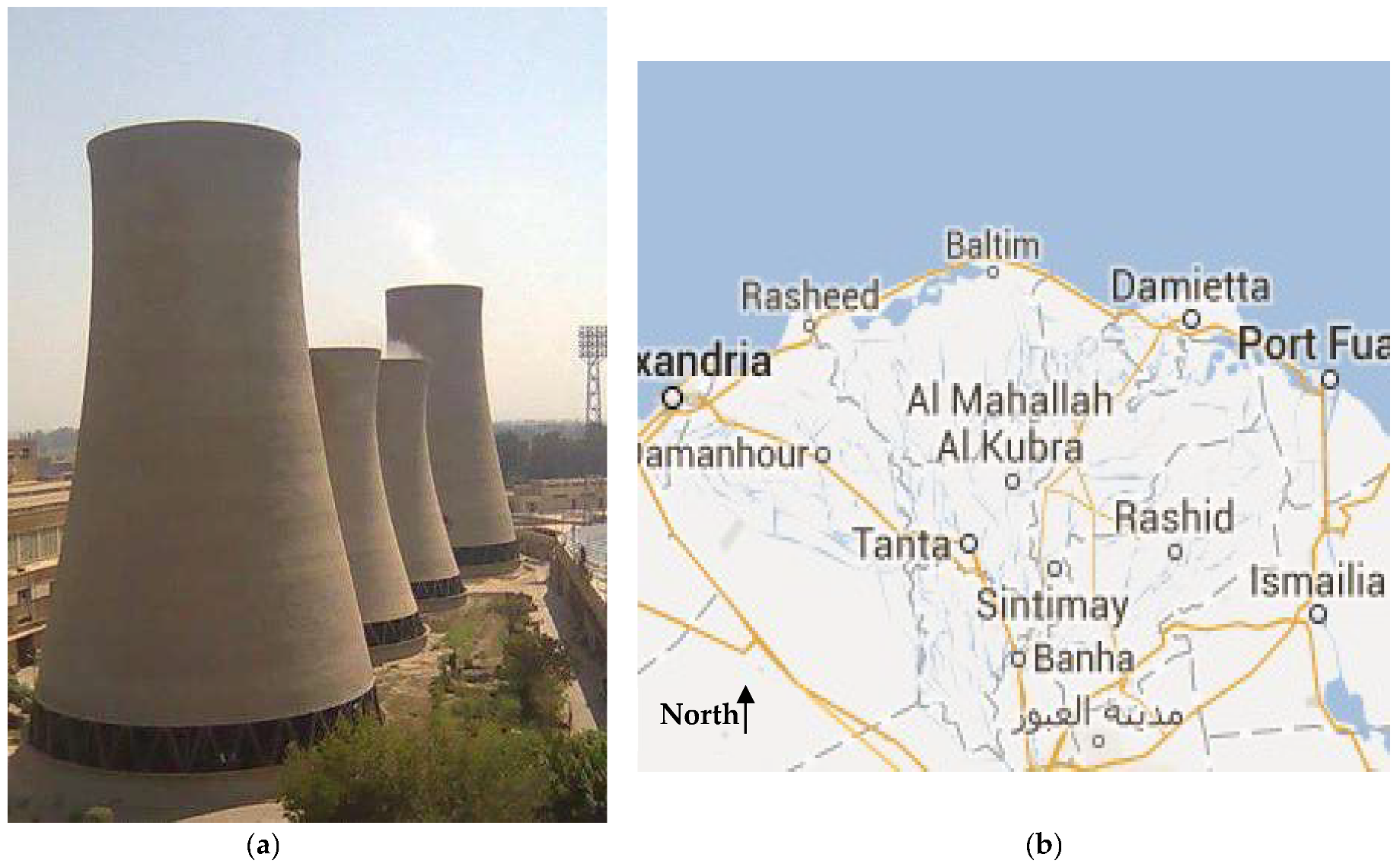
The studied four high rise cooling towers are located in El Mahalla El-Kubra city, Egypt. El Mahalla El-Kubra city (30.9687° N, 31.1665° E) is the largest city of the Gharbia Governorate in Nile Delta in Egypt. It can be considered the largest industrial and agricultural city in Egypt, located in the middle of the Nile Delta on the western bank of the Damietta Branch tributary, approximately 110 km north of Cairo and about 120 km from Alexandria. This city is one of the inner Nile Delta cities and its location is between the distance between Tanta, Kafr El-Sheikh and Mansoura cities, which is about 25 km from those cities (
Figure 1). The city is known for its textile industry, and hosts the Misr Spinning and Weaving Company (the largest cotton manufacturing company in Egypt) which employs around thousands of people. Misr Spinning and Weaving Company was founded in 1927s by the founder of the modern Egyptian economy, Mohamed Talaat Harb Pasha, which is located on 600 acres that includes housing, playgrounds and the factory which contains four cooling towers (the focus of this study).
These towers, as shown in
Figure 1, rely on the conversion diversion nozzle’s natural air draught to chill the water utilized in power plants, which is a simple process with low operating and maintenance costs. One of the towers’ maintenance can be performed while the other towers are being worked on. This system has the disadvantage of being more expensive to build and requiring a larger space than other mechanical cooling techniques.
Two of the studied four high rise cooling tower has approximately 56 m in height, and 38 m in diameter at the base and 21 m in diameter at crest. Both of them was constructed in 1959s, Czech industry. The other two cooling towers have approximately 40 m in height and 29 m in diameter at the base, and 16 m in diameter at crest. These towers were constructed in 1948s, English industry. The four studied cooling tower are made of reinforced concrete. The thickness of the tower wall gradually decreases from the bottom to the top where the thickness is 40 cm at base and decreases by height until the top becomes 12 cm. The tower is empty from the inside and open to the sky. The studied four cooling towers are dependent on the natural air withdrawal process, with the benefit of the choke area and conversion diversion nozzle. The pressure in the choke area is substantially lower than any other place far from the choke area when a fluid is moving at a rapid speed, and this difference in pressure between the two points is what triggers the natural withdrawal process 3000 m3/h of water must flow during the cooling cycle. Typically, just one of the four towers receives maintenance throughout the year, while the other three are operated, and so on, annually.
This type of structure is subjected to two types of loads, which are permanent loads and live loads. Permanent forces resulting from gravity, such as various types of weights, such as the weights of the structure itself and the weights of the elements concentrated on it permanently [
3]. Live loads to which these structures are exposed include climatic loads, earthquake loads, wind loads and loads resulting from heat, such as the internal air temperature resulting from evaporation and cooling process. These towers are located in El Mahalla El Kubra city. Egypt with a moderate nature in terms of the impact of earthquakes as well as the influence of winds and the effect on temperatures and the change in temperatures that contain these towers, the focus of our research in the second region of the areas of influence of earthquakes which the value of the design ground acceleration is 0.125 g. It is a small area of mild earthquakes over those areas. El Mahalla El Kubra city is considered one of the areas in Egypt where the wind effect is light. Each structure and every part of it must be designed and implemented to resist total horizontal forces that represent earthquake forces and cannot be ignored in areas subject to earthquakes.
3. The Applied Mathematical Models in the Reserach
3.1. Finding the Curvature Type and Equation of Cooling Tower Wall
For these structures (high rise cooling towers) to be safe and serve their intended purposes, accurate geodetic observation techniques are needed both during construction and once it is complete and start working (during operation). It is crucial to identify the cooling tower’s curvature type and equation in this section to determine the curvature type of the studied four cooling towers walls. In mathematics, a conic cross section is the intersection of a plane and a cone. A conic cross section’s general equation form can be expressed as [
1,
20,
21]:
The sign of the term (B
2 − 4AC) can be used to some extent to identify the cross section type. The curve is an ellipse, a circle, a point, or there is no curve if the sign of the equation (B
2 − 4AC) is negative. But if the term equals zero, the curve will be a parabola, two parallel lines, or not exist at all. If the term is positive, the curve will be a hyperbola or two intersecting lines [
20,
21,
22]. A, B, C, D, E, and F are the six unknown coefficients in Equation (1). As a result, the solution requires at least six points with X and Y values, but for n points in the same cross section, the principle of least squares theory must be applied [
23] to find the optimum values of these parameters and its accuracy.
From the principal of least squares theory, it deduced that:
where V
i is the residuals in observations.
Therefore, partial derivatives for Equation (2) must be performed and set to zero in order to obtain the coefficients (A, B, C, D, E, and F) at their optimal values and their accuracy as follows:
The following equations can then be generated in matrix form by differentiating Equation (3) with regard to parameters A, B, C, D, E, and F and equal to zero.
Equation (4) can be solved using the designed Matlab software program to determine the coefficients A, B, C, D, E, and F as well as its accuracy.
3.2. Determining the Verticality and Inclination of Circular Cooling Tower Using Geodetic Techniques
In this paper, two cases for determining the values of circular cooling tower inclination by using reflecorless total station, which has the ability to measure distances without prisms, are presented.
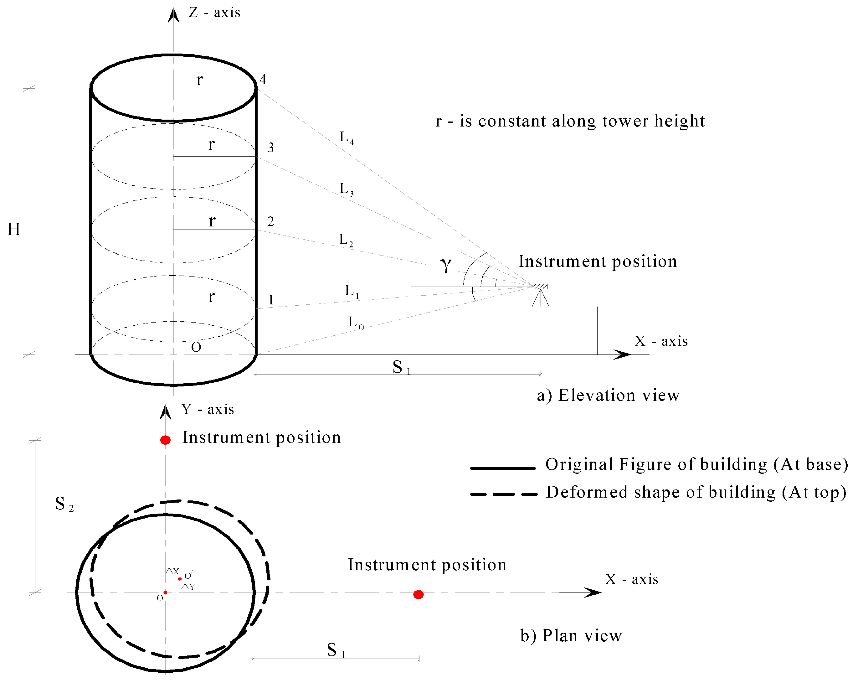
3.2.1. If the Diameter of Circular Cross Section of Cooling Tower Is Constant
The total station is fixed close to the structure (cooling tower) at distance (S) from its base, where it can be sight the full height of the observed tower as shown in
Figure 2. It is necessary to measure the slope distances and vertical angles spread at specific elevations along the height of the construction from the instrument to each horizontal section.
Therefore, the wall inclination value (Δ
i) at every point (i) along the height of the circular tower (H) can be calculated as follows:
where:
L0—The inclined distance from the instrument to the tower base;
Li—The inclined distance from instrument to section i along the height;
γ0, γi—Vertical angles from the instrument to the tower base and section i respectively.
Therefore, each section’s values for the circular tower’s inclinations must be established in the same manner for both directions. The accuracy of determining the inclination of the circular tower wall from a given direction increases with the number of points observed in that direction across the height of the tower.
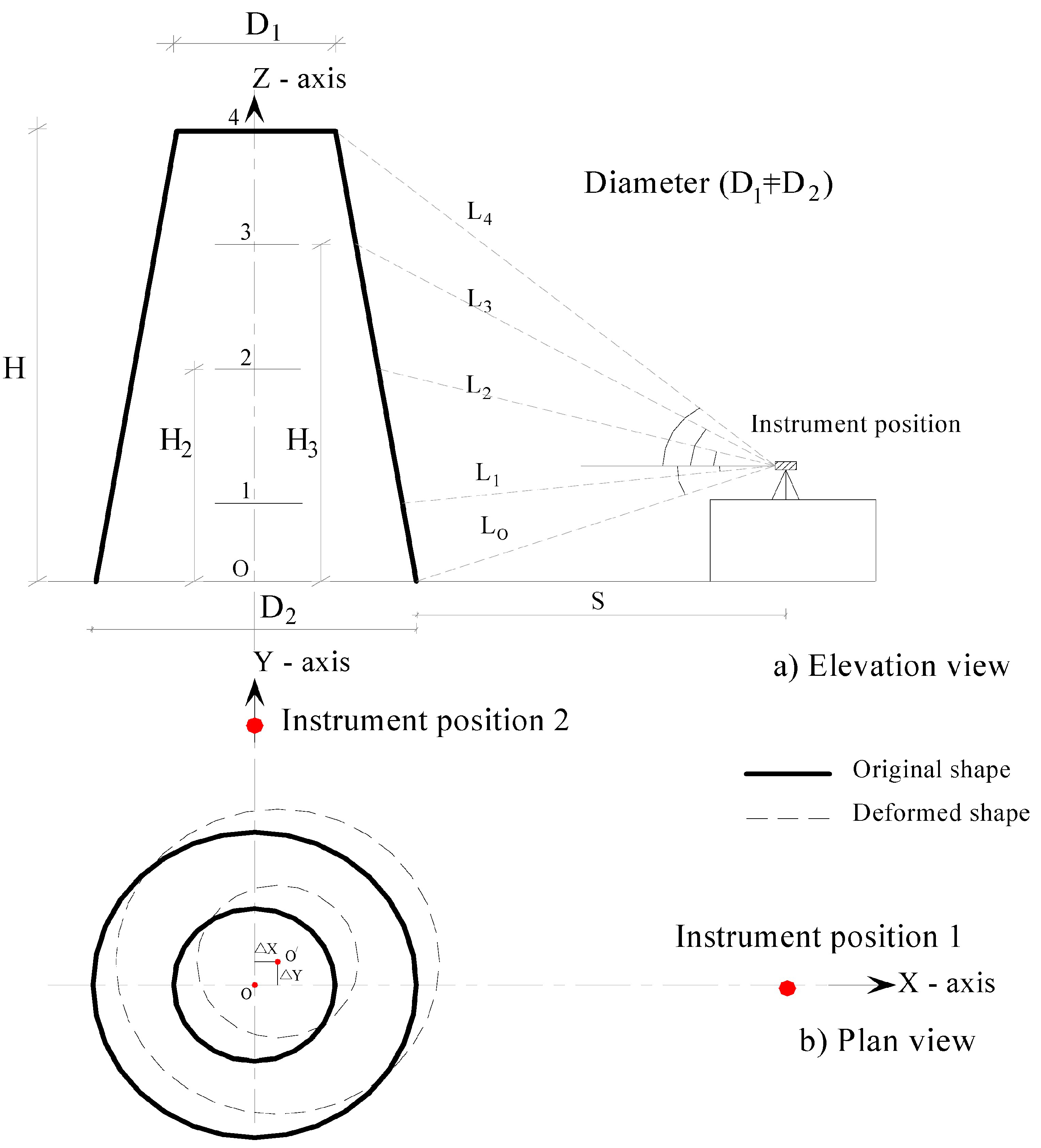
3.2.2. If the Diameter of Circular Cooling Tower Is Changed from the Upper to the Lower
The upper and lower cross sections of this type of cooling tower have different radii. This structure resembles a truncated cone in shape as shown in
Figure 3. The field work is the same for constant diameter circular tower. The applied mathematical models used to determine the values of wall inclination are the only distinction between them.
The following derived equation can be used to calculate the inclination value (Δ
i) at any section (i) along the tower height (H):
where:
γ0—vertical angel from the instrument to the tower base;
γi—vertical angel from the instrument to cross section (i) along the height of circular tower;
Di—the diameter of any section i along the height of tower;
D1—the diameter of top of the circular tower;
D2—the diameter of the bottom section (at base or foundation)
From the geometry of
Figure 3, it is deduced that:
where:
Then, for any height, the value of inclination (Δ
i) in either direction (X or Y) can be expressed as:
3.3. Finding the Radius and Center Coordinates for Circular Cross Section of Cooling Tower
The radius of the circular cross section (r) and the coordinates of the section centre (XC, YC) can be calculated using the method of least squares from the resulted coordinates of several points (more than three points) resulted from TLS observations on the circumference of a circular section as shown below:
Any observation point on the tower’s outer surface’s circular segment (X
i, Y
i) must conform to the following circle equation:
where X
C, Y
C, and r represent the circular cross section’s unknown center coordinates and radius, respectively. Equation (10), in which the observables and parameters cannot be separated, requires the general combined method of least squares adjustment [
23]. The general linear form of Equation (10) for n points resulted from TLS observations can be written as follows:
In which:
n = number of equations, where n is the number of monitoring points the same cross section;
u = number of unknowns; in this case u = 3; which are radius r and center coordinates XC, YC;
m = number of observations; in this case we find that m = 2 n;
A = matrix of partial differentials of Equation (10) with respect to unknowns (XC, YC, r) respectively.
B = matrix of partial differentials of Equation (10) with respect to (X1, Y1, X2, Y2, …, Xn, Yn) respectively;
L = vector of constant terms associated with each of Equation (10);
V = vector of the observed coordinates residuals.
The adjusted values of radius, centre coordinates, and their related accuracy must then be found using the combined least square approach. The theory of errors (generalized least squares) is then applied, a MATLAB program was created to determine the radius and the center coordinates for any circular section along the cooling tower height.
3.4. Determining the Circular High Rise Cooling Tower Axis Inclination from Circular Cross Section Radius Values and Coordinates of Center
The following steps summarize the suggested method for estimating the inclination of the circular cooling tower axis from circular cross section radius data and centre coordinates resulted from TLS observations analysis:
1. The height of the cooling tower must be divided into several horizontal sections at every 2 m for example or fewer to obtain the actual distorted shape of the cooling tower axis inclination. Each horizontal section will contain thousands of points coordinates resulted from laser scanner observations which cover the whole perimeter of the tower outer surface.
2. From the coordinates of the observed points obtained from TLS observations, the value of radius rj and the center coordinates for each 2 m along the cooling tower height must be calculated by using the least square method as presented in this paper.
3. By comparing the resulted center coordinates of subsequent cross sections with the center coordinates of the first circular cross section, one can determine the values and direction of the tower axis inclination as follows:
where
—center coordinates of any circular cross section j along the cooling tower height (H);
—center coordinates of the first section of the cooling tower.
4. Drawing the actual deformed shape of the cooling tower axis inclination from the resulted data obtained.
3.5. Projection of Observed Points Coordinates of Cooling Tower on Vertical Plane
The process of projecting the coordinate points obtained from TLS observations for the circumferential cooling tower’s outside surface is described in this section, with a description of how to use the derived equations to accomplish this goal. Two cases of the cooling towers are presented.
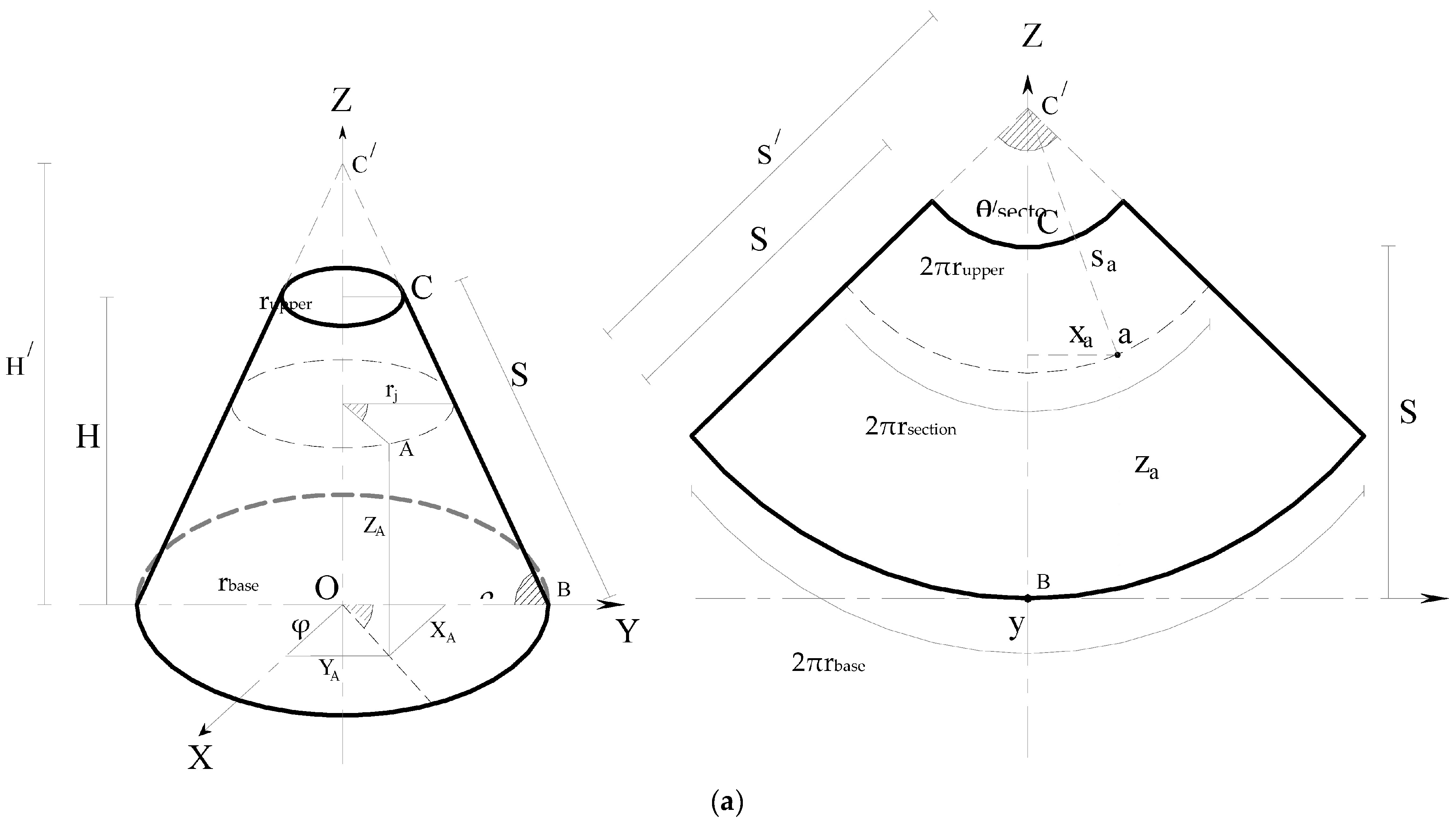
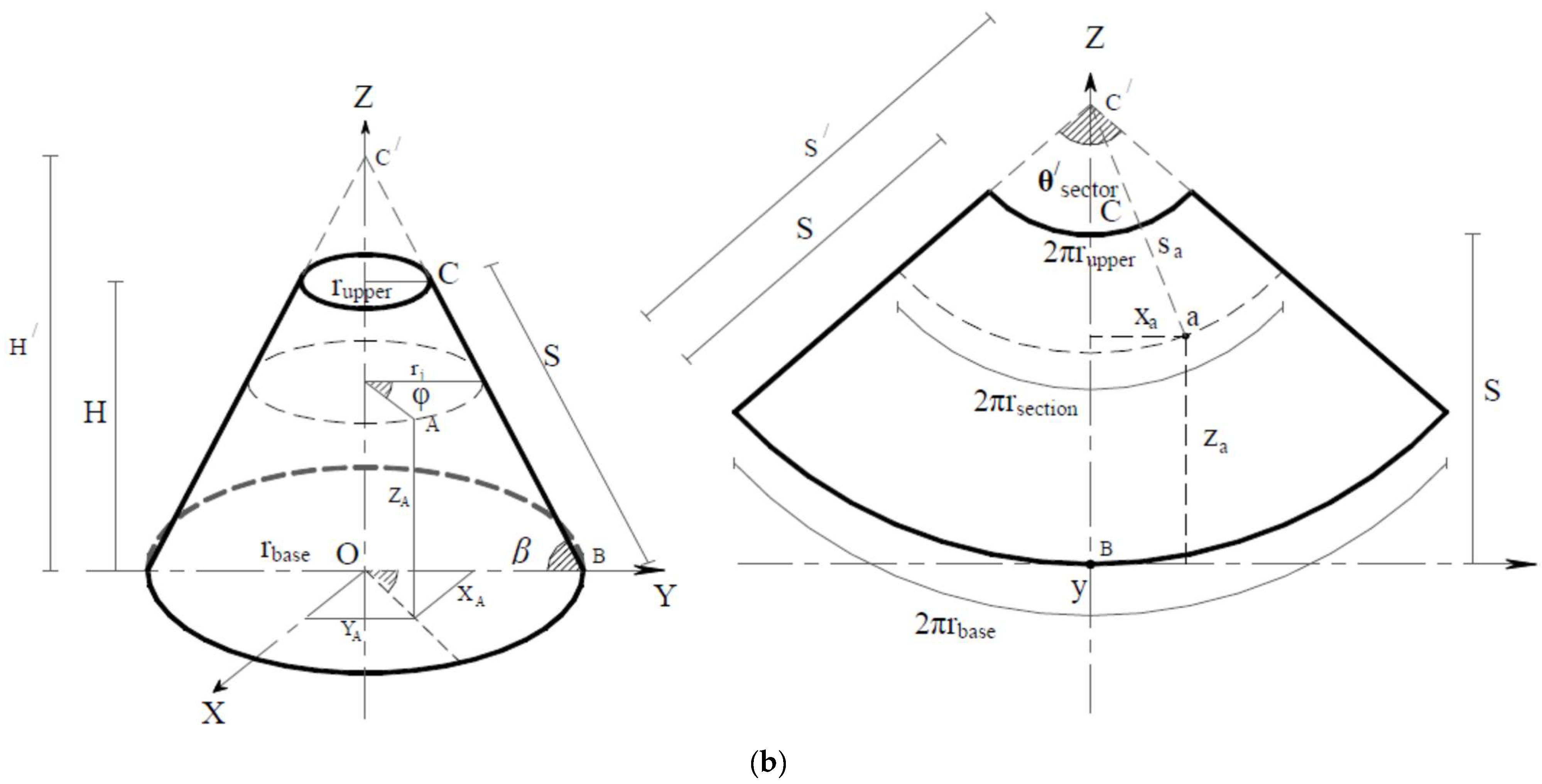
3.5.1. Cooling Towers Which Has the Form of Circular Truncated Cone
There are several cooling towers which have circular truncated cones in
Figure 4. The shape of a truncated cone cooling tower is obtained if a cone is cut off from the top by a plane parallel to the base. It is also obtained by rotating a rectangular trapezoid around its side perpendicular to the bases, or by rotating an isosceles trapezoid around the axis of symmetry. The circular truncated cone tower has two bases: the lower base of the original cone with radius (r
base) and the upper base of the cut off cone with a radius (r
upper) (
Figure 4a). The height of a truncated cone (H) is the perpendicular dropped from a point of one base to the plane of another. The suggested technique summarize that The deformation of this type of structure can be determined from terrestrial laser scanner observations (surface points coordinates) by projection of cooling tower surface points coordinates on vertical plane (
Figure 4b).
The inclination angle of truncated cone tower (
βTrun-Cone) can be determined from the geometry of
Figure 4, a as following:
Figure 4 shows the projection of truncated cone tower on vertical plane. The truncated cone has circular upper and bottom (base) sections with radius (r
upper) and (r
base) respectively. The expected figure from cone projection is shown in
Figure 4b. Slant height(S) of the truncated cone is the inclined distance from the circular upper section a cone, down the side to a point on the edge of the circular base section and equals (
). In
Figure 4b, the projected figure on vertical plane has sector central angle (
) and two curved lines; the upper one is the circumference of upper circular cross section equals (2πr
upper) but the second curved line is the circumference of base circular cross section and equals (2πr
base).
To determine the new coordinates projected on the vertical plane from the coordinates of the cooling tower outer surface resulted from TLS observations, the outer edges of the cone are connected and join to meet together at point C
/ (
Figure 4). Therefore, the resulting figure will be a complete cone with a new height H
/ equal to (
) and a new Slant height of the generating cone (S
/) has the form:
From the geometry of
Figure 4b, central angle (
) can be determined as following:
Based on the Cartesian coordinates of any observed point obtained from TLS observations of the surface of a truncated cone and depending on the geometry of the circle and cone (
Figure 4), the following derived formulas for calculating the length of the distance s
a of the point (a) and the angle in the plane (θ
a) can be drawn as:
Depending on Equation (16), the following equations for determining the new coordinates (x
a, y
a, z
a) of the projected points of the tower truncated cone surface onto the plane can be calculated as following:
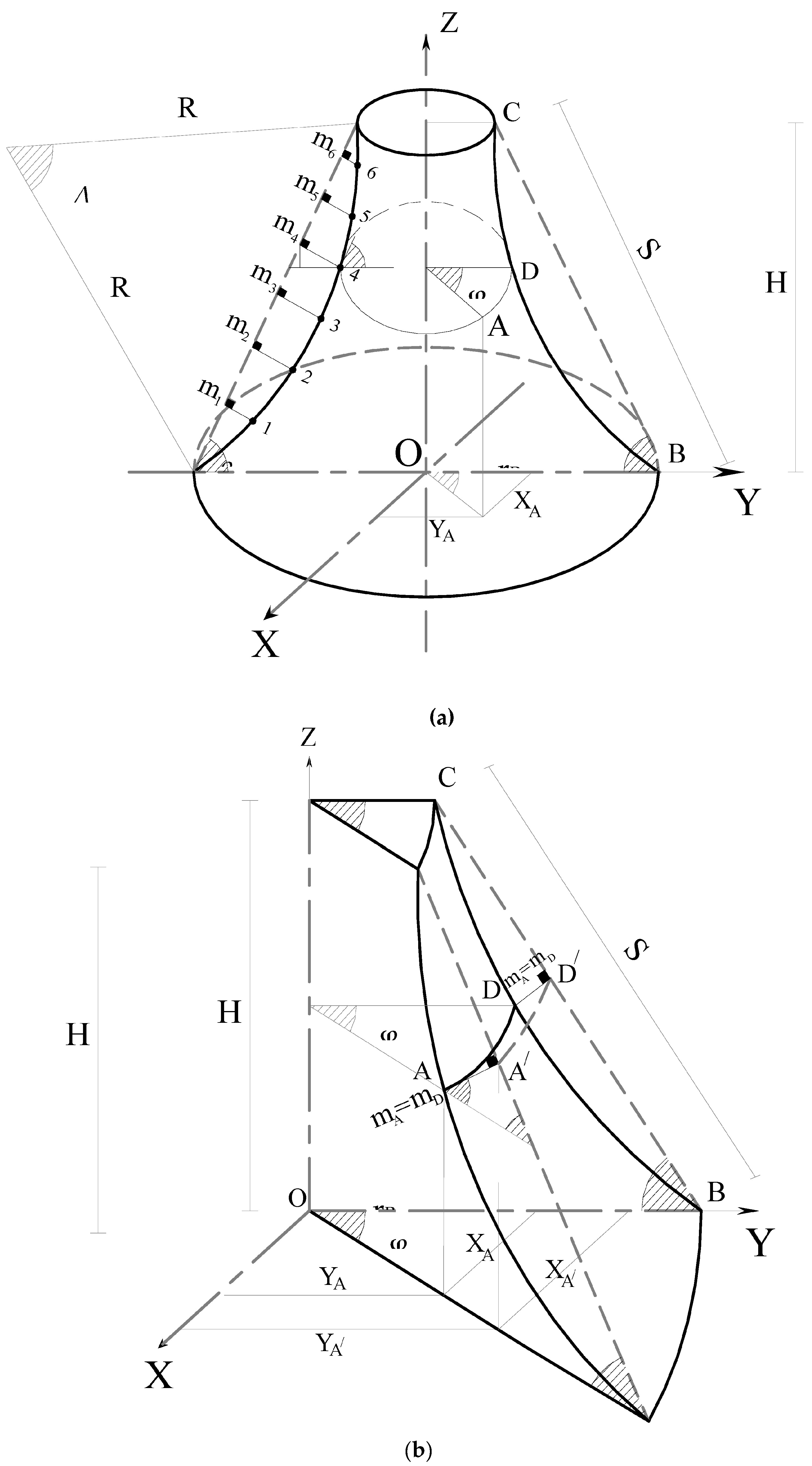
3.5.2. Cooling Tower Which Have Truncated Cone Shape with Curved Wall (Studied Cooling Tower)
This type of structures (studied cooling tower) consists of two parallel bases in the shape of a circle with two different radii and is defined as a figure formed by second-order curves with radius R as shown in
Figure 5. This type of structure can be considered a special case of a truncated cone with curved wall. The results of observations of these structures using terrestrial laser scanner are point cloud containing three-dimensional coordinates of points on the outer surface. This paper presents a method for determining the deformation in the outer surface of this type of structure through projection of surface coordinates resulted from TLS observations onto vertical plane. The main types of second order curves are circle, ellipse, parabola and hyperbola. Each type of them has its own property, which is often mistaken for the definition of a curve. A circle can be defined as a special case of ellipse. A method is presented for transforming the points of the lateral surface of these structures with a generatrix of a circular section, which has a radius R (
Figure 5), into a vertical plane. This type of structure is projected on a vertical plane by two basic stages:
The first: Projecting the coordinates of the observed points (real TLS observations) located on the surface of the structure into a truncated cone, where the walls are straight and not curved.
The second: Projecting the new coordinates of the observed points converted into a truncated onto a vertical plane, followed by finding the equation of this plane and determining the deformation value for each point on the formed plane.
As shown in
Figure 5a, from several observed points (points No. 1,2,3, …,
Figure 5a), which are located on the same vertical section of the wall surface, the radius of the circular section R is determined using the least squares method as mentioned above in this paper. It can be seen also that the length of the chord BC is equal to the slant length (S) of the empirical truncated cone and is equal to
. Then, the central angle of the curvature wall of cooling tower (Δ) can be determined by the formula
To transform the coordinates of the observed points on the lateral surface of this structure into an empirical truncated cone, it is necessary to construct the orthogonal distance mi from each observed point to the cone (
Figure 5). The maximum value of the orthogonal distance mix. reaches the height of the structure in the middle
and is equal to
. Therefore, using the geometry of a circle, one can obtain the following equation for determining any orthogonal distance mi from each observed point to the cone
Depending on the calculated horizontal angle (φ
i) at each observed point and the orthogonal distance mi (
Figure 5), it is possible to transform the coordinate of any point into a truncated cone according to the formulas
where
are the coordinates of the point on the cone;
are the coordinates of the observed point.
Then, the empirical truncated cone can be unfolded onto a plane by a similar method of unfolding a truncated cone. It should be noted that this method of transforming the coordinates of the points of the lateral surface of a structure with a generatrix of a circular section into a truncated cone turns off distortions. The distortion of any vertical section of the lateral surface of the structure is that the actual circular distance BC is projected as a straight distance S per cone, so the amount of vertical section distortion can be determined as the difference between the two circular and straight distances. The maximum amount of distortion is . However, the distortion of any horizontal section arises from the difference between the actual value of the radius of the circular section of the structure and the designed value of the radius on the cone. The amount of distortion of any horizontal section is .
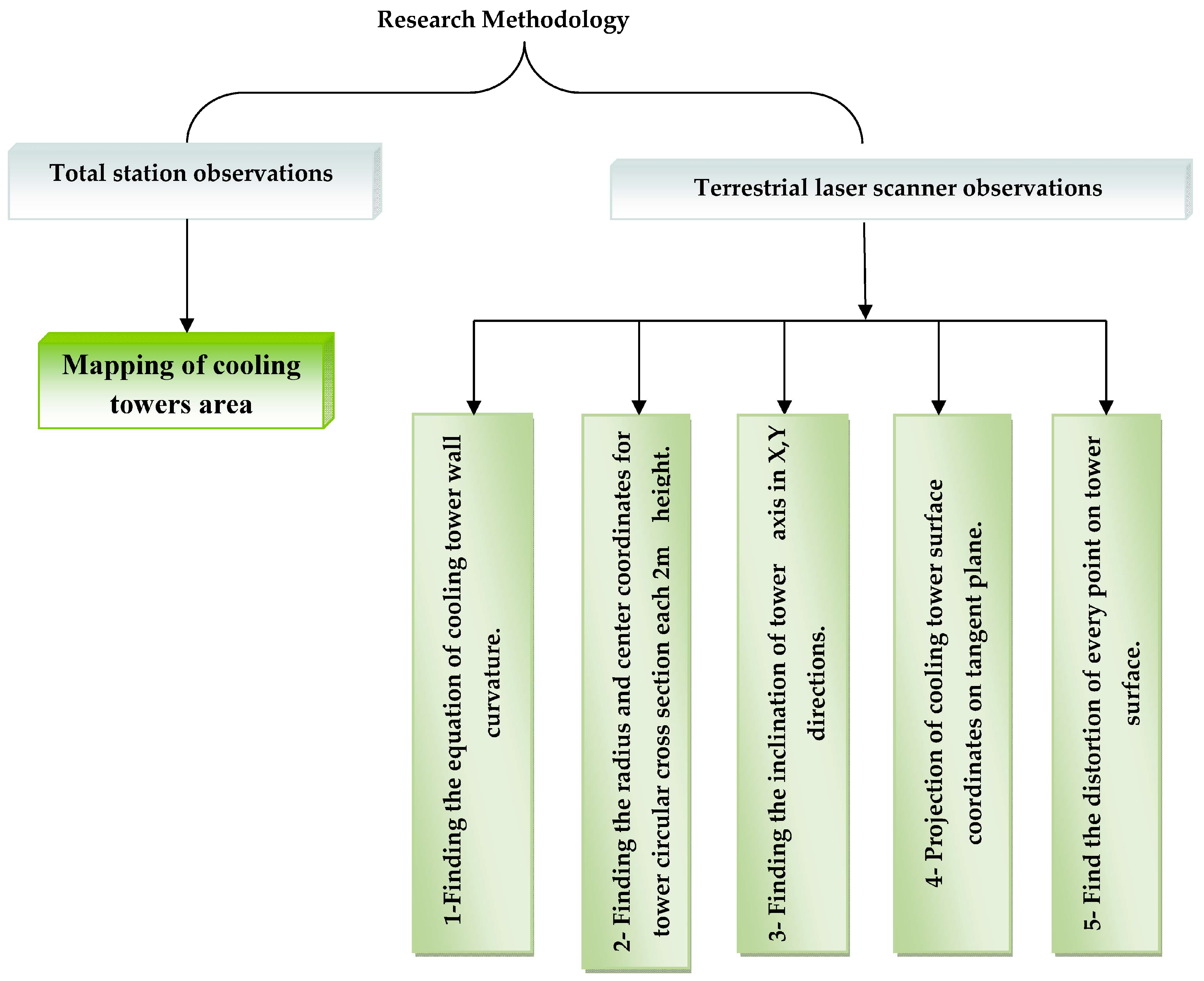
4. Research Methodology and Plan
The process flow for this research is depicted in
Figure 6, from site mapping of the study region to data collecting, processing, and analysis of TLS observations to identify the deformation and distortion of the studied high rise cooling towers.
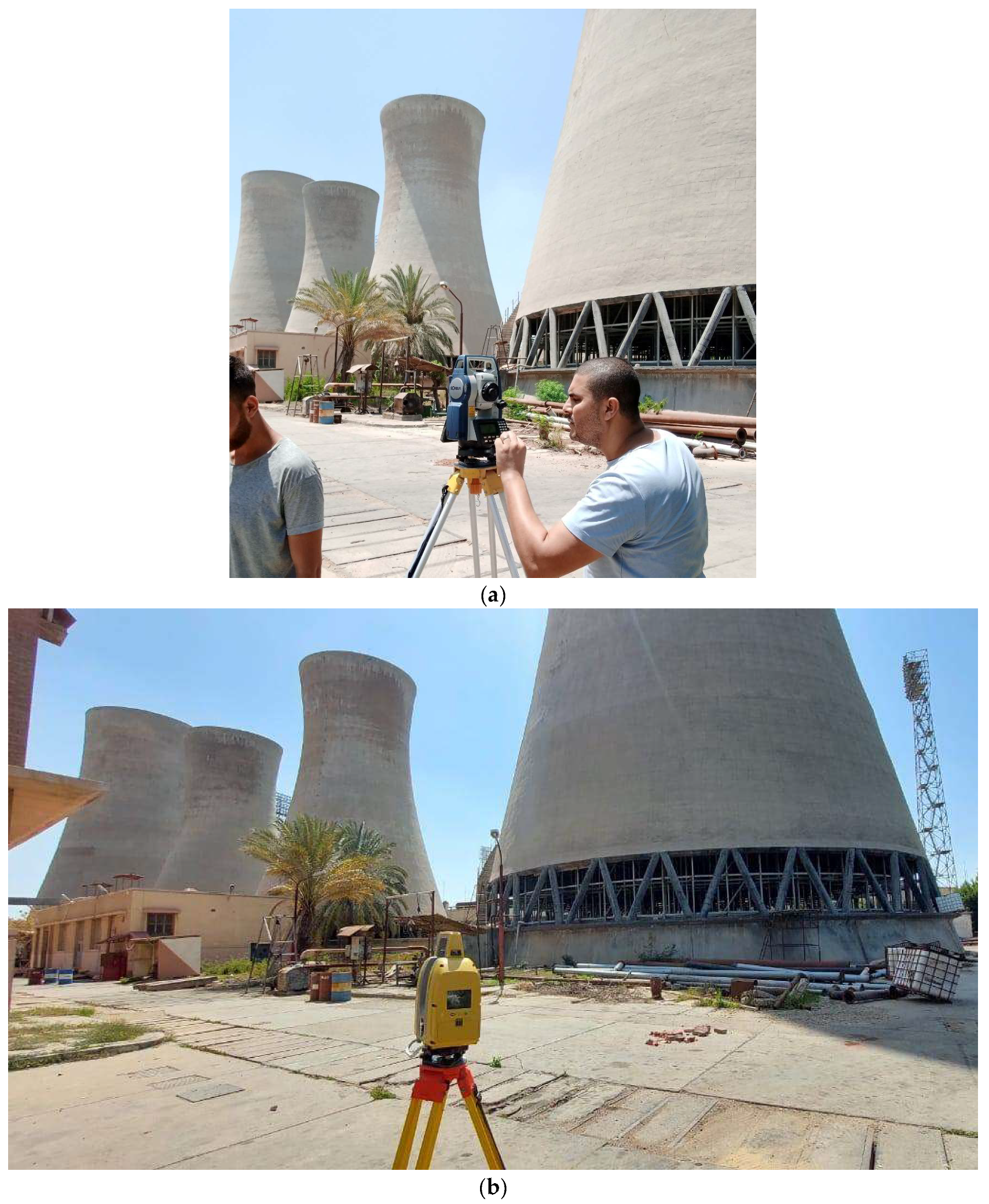
5. Field Work and Data Collection
The used instruments were reflectorless total station (Sokkia) with accessories and Topcon GLS-2000 3D (Tokyo, Japan) terrestrial laser scanner. The used total station has a standard division 1” for angle measurements and ±(2 mm + 2 ppm × D) for EDM measurements with reflector and ±(3 mm + 3 ppm × D) for EDM measurements without reflector
Scanning distance of the used laser scanner can reach up to 350 m distance from object. The distance accuracy reaches 2 mm (for distance 150 m). It lasts about 18 min maximum time to obtain more than 5 million scanned point cloud with a 6 s angular resolution. Compensation range ±6 min and target detection accuracy 3 s at 50 m. Total station was used for mapping cooling tower area. When performing measurements, the influence of external conditions, which is systematic, was taken into account.
A cadastral map of the study area was first created by surveying the area around the towers using the specified total station. Constants (fixed points) were then imposed to connect all of the total station’s occupied stations and create a single one coordinate system. To minimize time and effort, the optimum instrument positions were selected as shown in
Figure 7. Then, until the full completion of all cadastral work, the total station was transferred and connected to the imposed constants. The Autodesk Civil 3D program was used to illustrate the comprehensive drawings of the research area and to establish the geometric dimensions of the cooling towers after the observations were processed.
The four high rise cooling towers have been scanned using a TLS Topcon GLS 2000. Before using TLS, there are a few configuration tasks. Firstly, to undertake data post-processing, the target scan needs to be aligned with the spot information of several 3D scanning datasets. As a result, the target was positioned so that it could be visible from every scanner position at the subsequent station. The target was positioned close to the scanning target in order to measure the object (four cooling towers). At least three different sets of common target data must be scanned in order to align the positional information to the data. In order to parallel each station, the target was set up in four positions.
To completely cover the perimeter of the outside surface of the studied four cooling towers, four standard mode scans were conducted from various locations around the towers. Each scan had a varied resolution, scan time, and resulting point cloud count. The MAGNET COLLAGE program was used to process the data collected from TLS observations [
24], which also helped us estimate the accurate coordinates of the outer surface of all cooling towers as shown in
Figure 8.
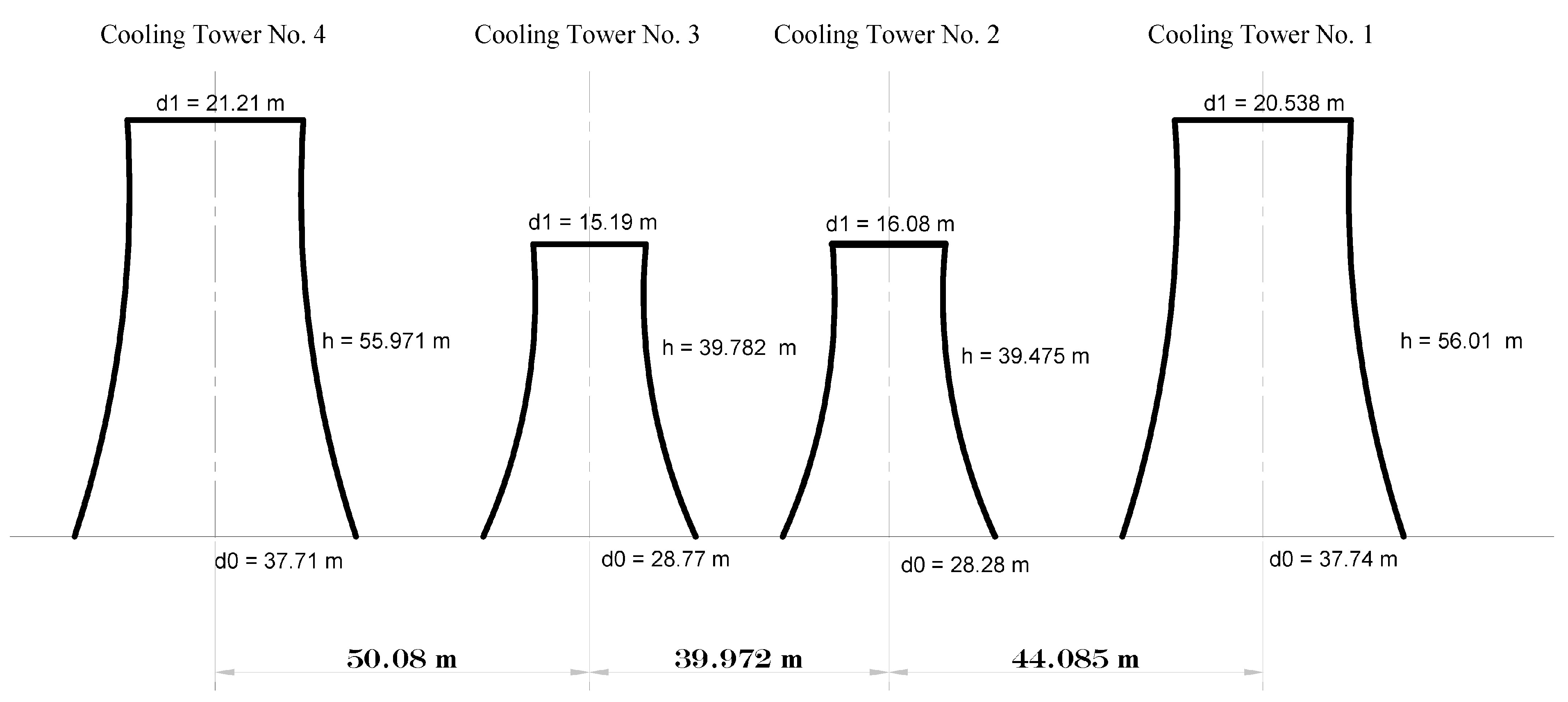
Depending on the results of field work, geometric properties of the four studied cooling towers are determined accurately using TLS observations. These geometric parameters include tower heights, tower diameters (base diameter and top diameter), and the distances between towers. The results of these parameters resulted from TLS observations can be illustrated in
Figure 9 and
Table 1.
6. Study the Accuracy of Terrestrial Laser Scanner Observations for Deformation Monitoring
Any monitored building or structure such as circular oil tanks and cooling tower can anticipate small vertical or horizontal movements, frequently measured in millimetres or centimetres, as known [
25,
26,
27,
28]. To successfully and confidently detect exact and accurate point movement, it was critical to assess the sensitivity and accuracy of the terrestrial laser scanner (TLS) observations in detecting the deformation of deforming objects. To achieve this purpose, the following laboratory test is performed.
The following test was run to determine the performance of terrestrial laser scanner (TLS) under circumstances similar to those expected during construction of the actual detectors. The suggested test evaluates the accuracy of the instrument inside a reference frame created by a series of incredibly accurate control measurements.
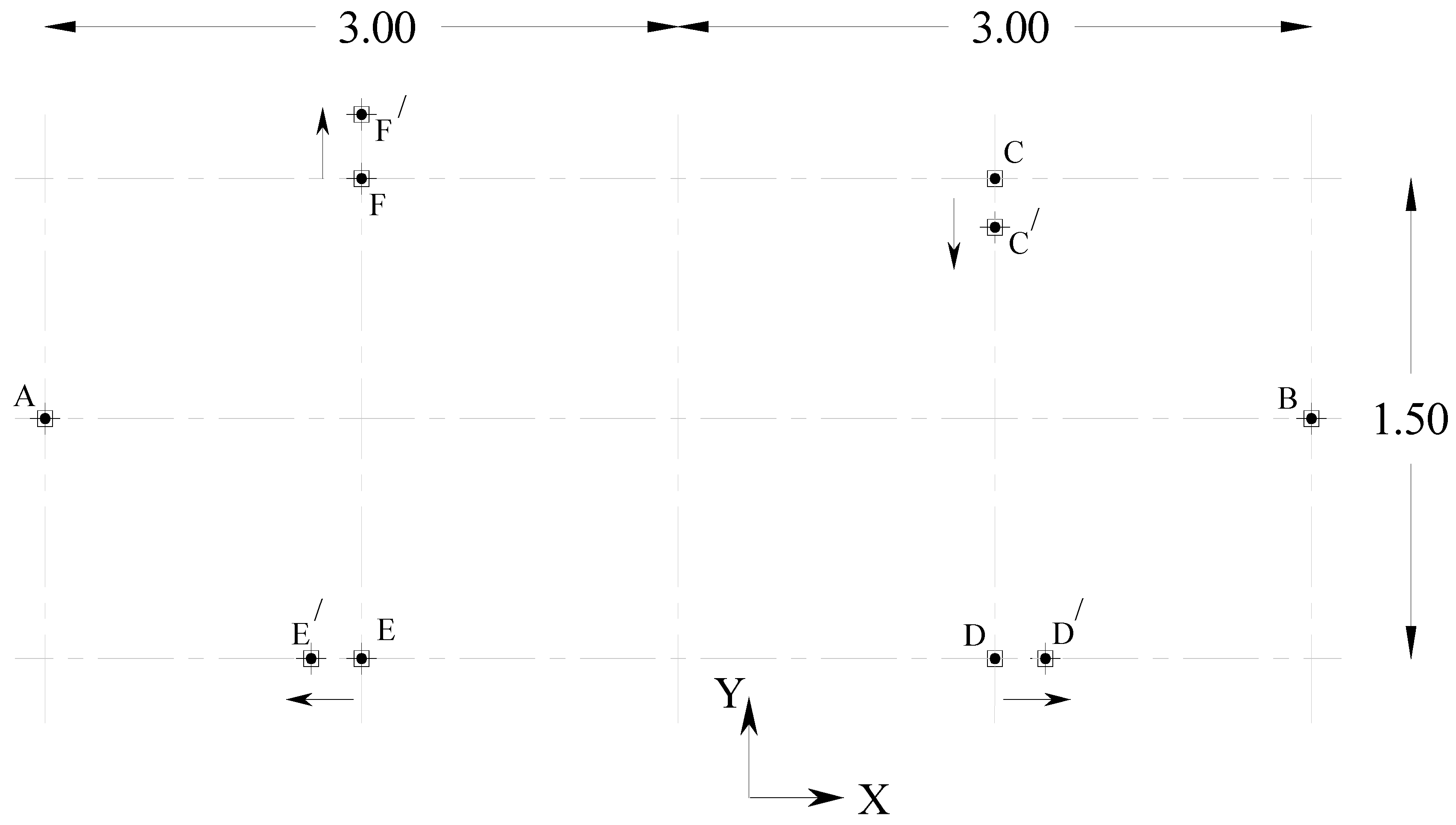
Six targets (A, B, C, D, E, and F) were mounted on a vertical wall.
Figure 10 depicts the distances between markings. Before the test, the distance between the targets was measured with a highly accurate device such as vernier. The required TLS was positioned roughly 6 m away from the wall for all observations epochs (scans) and fixed with the same resolution for all scans and observations epochs. A short distance was chosen between TLS and the wall to minimize any errors as much as possible that may result from the long distance so that the difference in coordinates between scans becomes an expression of the actual displacement between points. The test is carried out indoor to avoid any weather or natural errors. The accuracy of distance and angle measurements taken into consideration in calculation. The two markings A and B will remain constant throughout all observation epochs (scans). As a measure of control against the two deforming targets, these two fixed targets (A and B) were provided.
The primary concept of the experiment is that the two targets A and B will remain fixed while the four targets at points C, D, E, and F in
Figure 10 be moved by known distances in the directions X and Y (two separate directions) by changing values. As illustrated in
Figure 10, points D and E will be moved horizontally in opposite directions while points C and F will be moved vertically in opposite directions as shown in
Figure 10. A vernier with an accuracy of 0.02 mm was used to measure the displacements in both vertical and horizontal directions for all epochs. In all scans, the resolution of the scanner observations is fixed.
The first deformation analysis involved moving the targets by several increments values for points C and F (as vertical movement, direction Y,
Figure 10) and for points D and E (horizontal movement, direction X,
Figure 10). For each targets movements (simulated as observations epoch), the six targets were observed by the specified TLS and the distance between targets were measured by vernier.
By comparing the values and accuracy of the calculated distance between observed targets derived from coordinates measured by TLS and the measured distance from another accurate instrument (vernier with accuracy 0.02 mm), it is possible to assess the accuracy of TLS. The length of side, from its end coordinates (Points i and j) can be calculated by:
The accuracy of the side length between two points can be computed based on the accuracy of distance and angles by differentiating Equation (21) and applying propagation law. Each point’s deformation and accuracy for each epoch (C, D, E, and F) were computed. The final results are listed in
Table 2.
Table 2 shows that the difference of measured distances between the two points (simulated as deformation value) resulted from vernier and TLS is small. Maximum and minimum values for the difference are 2.12 mm and 1.18 mm respectively.
Therefore, it is evident from the outcomes of this laboratory experiment that the terrestrial laser scanner, in addition to its main advantage in remote monitoring without physical contact with the monitored target or building, can measure distances with acceptable and sufficient accuracy in the field of monitoring and observing engineering structures.
7. Results and Analysis
The noise from the field TLS observations was removed using the MAGNET COLLAGE program, and all the coordinates resulting from TLS positions were connected into one coordinate system, with the accuracy of the observations and coordinates being determined. In this section, the important results of the research will be presented.
7.1. Determine the Curvature Equation of Cooling Tower Wall
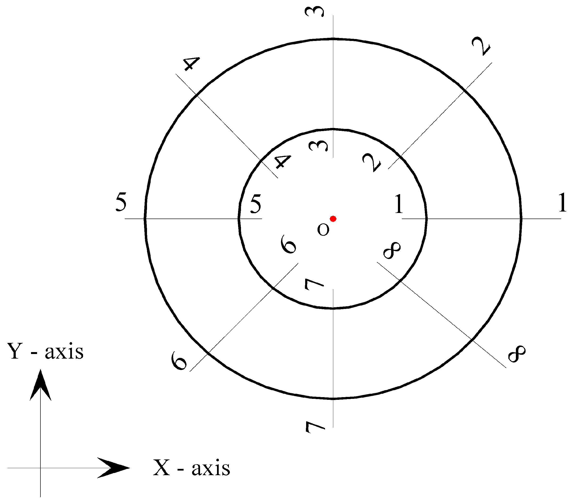
It is necessary to identify the curvature type of the cooling towers walls in order to apply the suggested technique to determine the deformation of the studied cooling towers with curved walls. In order to establish the type of curvature, the outside circumference of each tower was divided into a number of vertical sectors as shown in
Figure 11, and the coordinates obtained from the laser scanner observations were dealt with in each sector. By using Equation (4), the six parameters of conic section for all sections for cooling tower No. 1 depending on the coordinates are presented in
Table 3.
From the results presented in
Table 3, which were computed using Equation (4) and the created MATLAB program, it os deduced that the values of term (B) are too small and can be neglected, and the term (B
2 − 4AC) is always negative. Therefore, the walls of the towers are a straightforward circular curve (a portion of a circle).
7.2. Radius and Center Coordinates of Several Circular Cross Sections for Cooling Towers
The coordinates of each cooling tower are collected with one system coordinates. Depending on the laser scanner observations, which are cloud of thousands of points coordinates, for outer surface of cooling tower surfaces, the coordinates for surface are divided each 2 m along the tower height. The center coordinates, cross section radius and its accuracy are calculated for each 2 m height for each cooling tower using least squares as presented above using the designed Matlab programming.
Table 4 shows the calculated radius and center coordinates and its accuracy for all sections of cooling tower No. 1.
From
Table 4, the following remarks can be drawn:
1. The radii of cross sections of cooling tower No. 1 are varied along the tower height. The maximum tower cross section radius value is 18.5761 at height 2 m and the minimum value is 9.6675 m at tower height 50 m with average value of radius 13.108 m. The accuracy of cross section radius values ranges from between 0.9 mm and 2.8 mm with average value 1.92 mm.
2. The difference between center coordinates of all sections is small with maximum difference value 29 mm in X direction but 36 mm in Y direction
7.3. Inclination of the Cooling Tower Axis
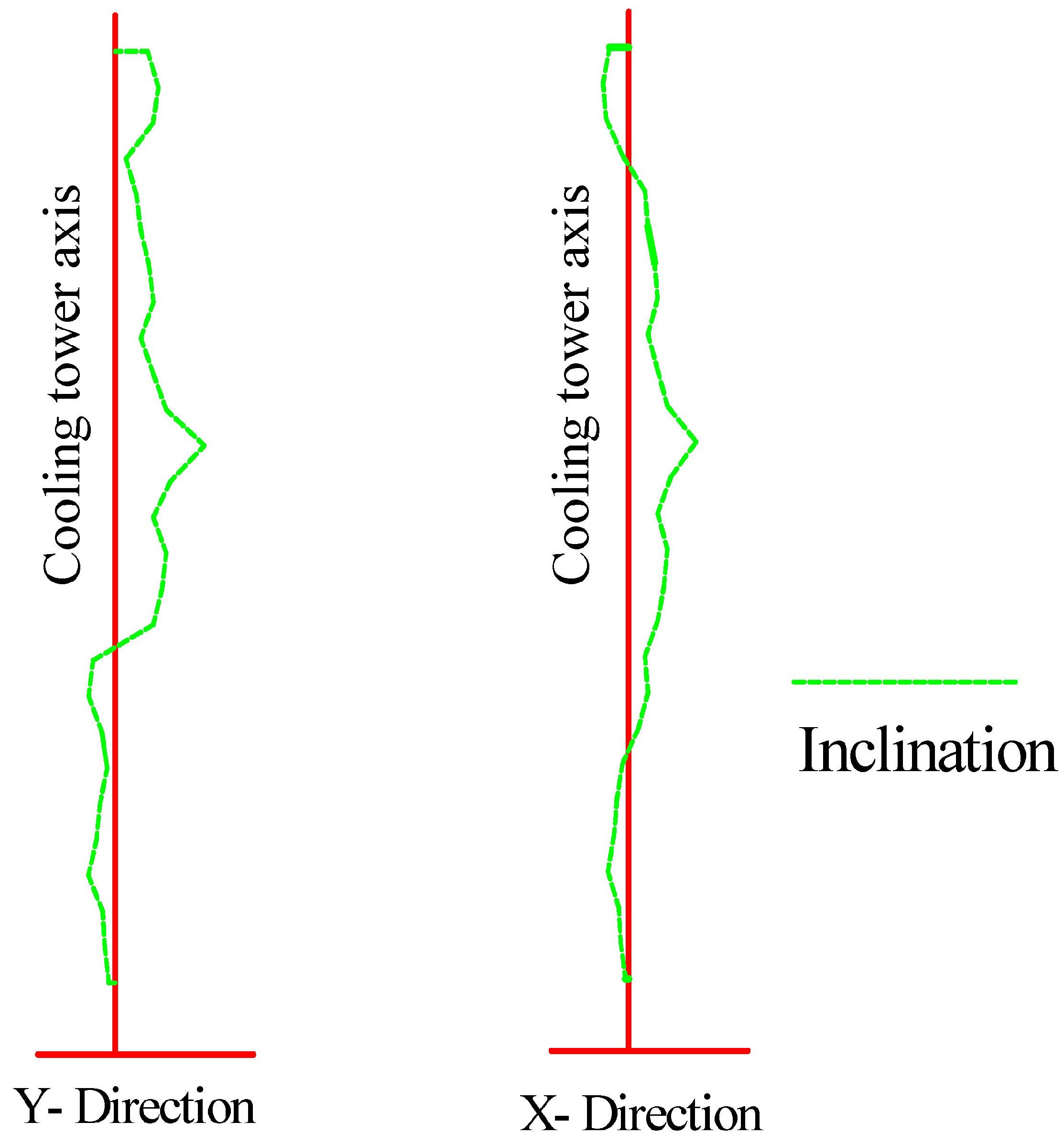
Depending on the values of center coordinates of all cross sections, the tower axis inclination for tower No. 1 can be determined as discussed above. The results are drawn in
Table 5 and
Figure 12 for cooling tower No. 1 as an example for proposed technique. The same procedure can be done for any other tower.
It is clear from
Table 5 and
Figure 12 that the values for cooling tower No. 1’s axis inclination vary while these values fluctuate with tower height. At a height of 34 m from the tower base (the level of the land next to the tower), it is discovered that the maximum value of the inclination in the X direction is 21.4 mm, and the lowest value of the displacement in the X direction is −7.3 mm at a height of 54 m. However, it is deduced that the direction Y has a maximum value of 27.8 mm at a height of 34 m from the tower base and a lowest value of −8.3 mm at a height of 10 m. This indicates that at height 34 m of tower height, there is clear inclination in the two directions. Therefore, the effectiveness of applying and using the method described by the study in monitoring and determining the inclination of the axis of any circular-section engineering constructions is obvious from these data and findings.
7.4. Deformation of Cooling Tower Using Projection of Surface Points Coordinates on Plane
The steps of determining the deformation of cooling tower walls using the suggested technique can be summarized in the following:
1. The observations collected by the used laser scanner are processed using MAGNET program and output in the form of three-dimensional coordinates in one coordinate system for the outer surface of the cooling tower.
2. The resulting coordinates of the cooling tower surface are projected onto a vertical plane using the equations presented in this paper.
3. The equation of the projected plane is determined though determining the coefficient of the plane and its accuracy using least squares technique as presented.
4. The orthogonal distances (∆i) for each i-the point to the fitted plane were calculated to determine the distortion of the fitted plane which can be considered as deformation of cooling tower.
Determining the plane equation from n points can be found in [
1,
3] using least squares estimation. The orthogonal distances (∆i) for each i-th point to the fitted plane can be found also in [
1,
3]. For cooling tower No. 1 (as a sample), all the steps were done carefully up to finding the orthogonal distances (∆
i) for each i-th point of the coolinf tower wall surface.
The resulting displacement values (orthogonal distances (∆
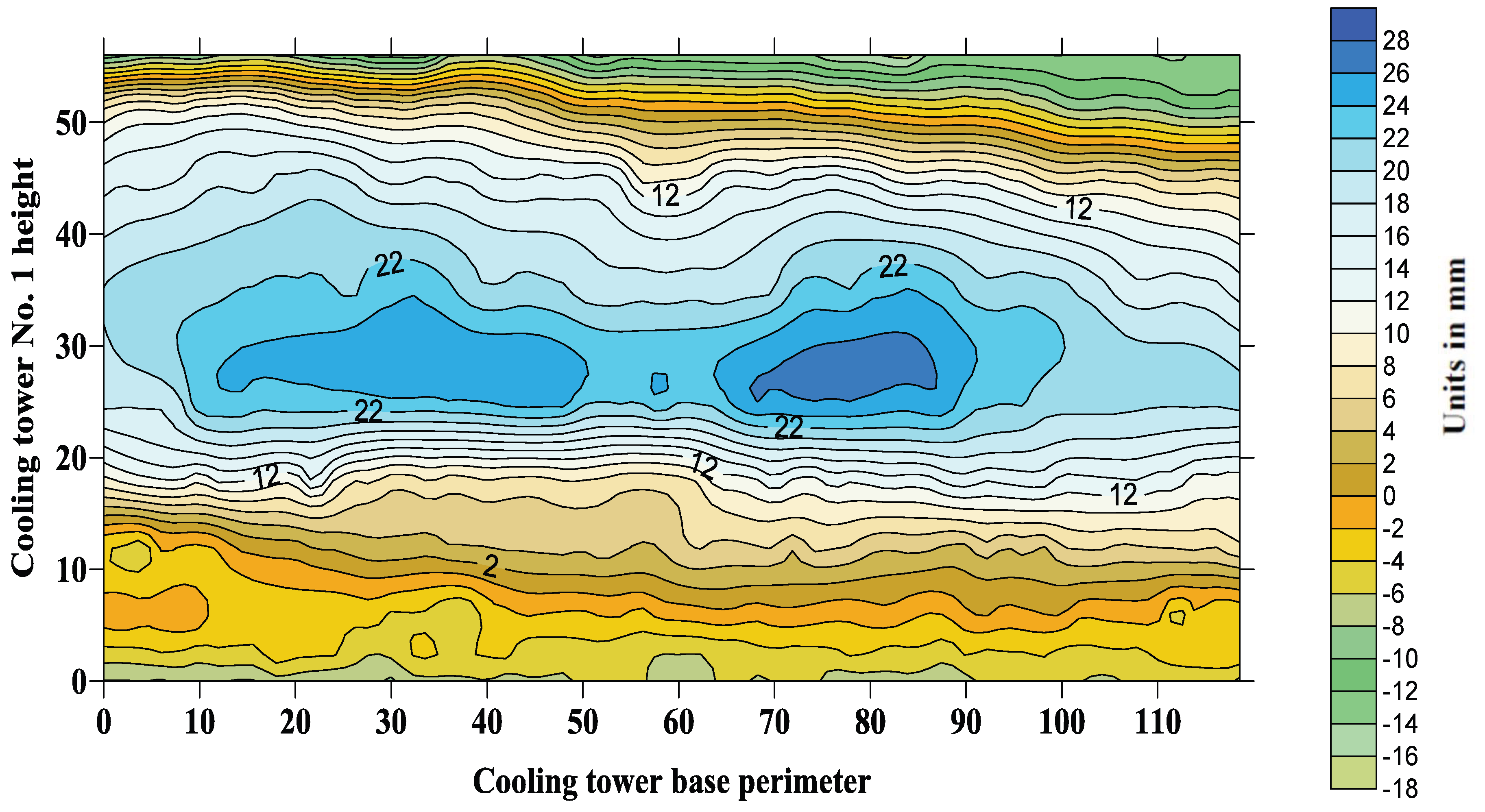
i)) were drawn in a contour map using Golden Software Surfer version 26.1.216 that expresses the deformation values of the outer surface of the tower, which can be represented as a digital elevation model (DEM) of tower deformation as shown in
Figure 12.
The internal contour lines in
Figure 13 represent the deformation (distortion) values in mm for each point on the cooling tower’s outer surface, while the horizontal axis represents the cooling tower’s circumference in meters (the perimeter of the lower base of the tower). The vertical axis represents the tower’s height (H) in meters. According to the
Figure 13, the part of the tower that is most susceptible to deformation is in the centre, at a height of about 30 m, where deformation values vary from 20 to 28 mm.
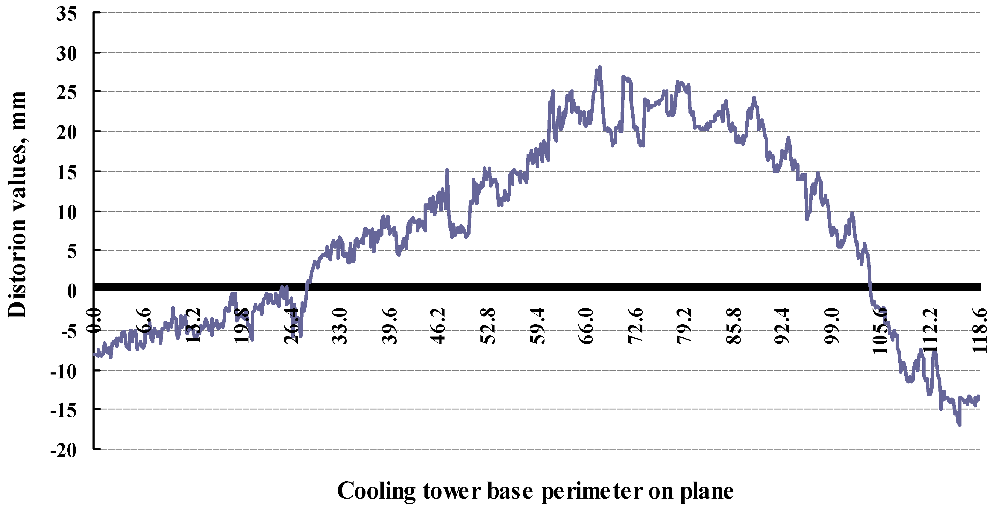
Figure 14 shows the deformation values which represents the orthogonal distances (∆
i) to a suitable plane for cooling tower No.1, where horizontal axis represents the cooling tower’s circumference in meters but the vertical axis represents distortion (deformation) values (∆
i) in mm.
The results from
Figure 14 support those from
Figure 13 because the maximum distortion value is between 25 and 28 mm, which are much higher than the precision of measuring the coordinates produced by TLS. As a result, the observed cooling tower (tower No. 1) exhibits the greatest deformation in the region’s middle.
The proposed geodetic method for monitoring the structural deformation (monitoring using terrestrial laser scanner, data processing, and projection on a vertical plane) is considered better than other alternatives methods used in monitoring deformation, whether geodetic or geotechnical methods, whereas it is characterized by creating a three-dimensional model and a large amount of data (3D coordinates) of the external surface of the structure in addition to contactless with the observed structure.
8. Conclusions
This paper investigates the possibility of using terrestrial laser scanner in determining the deformation of high rise cooling towers through projection of outer surface coordinates resulted from TLS observations on vertical plane. The paper presents also a practical techniques and mathematical method for determining the inclination of circular cooling tower axis through calculating the radius and center coordinates for different cross sections along tower height. A method for determining the type of cooling tower wall curvature using least squares technique is also presented and discussed. From the presented models and analysis, it is deduced that:
1. In comparison to other geodetic or geotechnical techniques and instruments, the terrestrial laser scanner (TLS) can observe and monitor high-rise circular cooling towers with acceptable accuracy for structural health monitoring and deformation determination because it can do so without coming into contact (contactless) with the monitored object (structure). There was great difficulty in determining the deformation that occurred to this type of engineering structures (high rise cooling tower with curved wall) due to several considerations, the most important of which is the curvature of its walls and its extreme height, but with the presence of this instrument (TLS) and using the suggested data processing and analysis, the matter became easier and possible.
2. The results of practical and analysis works obtained in addition to the method of data display and the results following processing the data of TLS and applying the suggested method, which is projecting the coordinates of the wall outer surface points of the tower on a vertical plane, confirm the efficacy and significance of this method with the possibility of applying it to engineering structures with circular sectors, such as water and oil tanks, minarets, and chimneys.
3. Because there are obvious deformation values in cooling tower No. 1, maintenance work must be included. The tower must be checked and monitored several times at brief intervals to guarantee the stability of the inclination values.
4. In order to maintain the safety and security of these engineering constructions (high rise cooling towers); it is necessary to define a periodic monitoring system as well as to establish engineering controls and standards.
It is recommended from the presented paper that high rise chimneys and building with circular façade and circular oil tanks must be monitored by the suggested geodetic techniques in observations and data analysis. More researches are required, however, to fully understand all error sources and their influence on terrestrial laser scanning system results for achieving high precision deformation surveying.
Author Contributions
Conceptualization, Ashraf A. A. Beshr; methodology, Ashraf A. A. Beshr; software and validation, Ali M. Basha and Fathi Abd El-Azeem; formal analysis, Fathi Abd El-Azeem; investigation, Samir A. El-Madany; field works and resources, Samir A. El-Madany; data curation, Ashraf A. A. Beshr; writing—original draft preparation, Ali M. Basha; writing—review and editing, Fathi Abd El-Azeem. All authors have read and agreed to the published version of the manuscript.
Funding
This research received no external funding.
Data Availability Statement
All data, models, and code generated or used during the study appear in the submitted article.
Acknowledgments
The authors extend their sincere thanks to Mohamed Hamed, as well as the Engineering Survey Laboratory, Faculty of Engineering, Kafrelsheikh University, for their assistance and contributions in the practical and field works of this research.
Conflicts of Interest
On behalf of all authors, the corresponding author states that there is no conflict of interest.
References
- Beshr, A.A.A. Monitoring the Structural Deformation of Tanks; LAP LAMBERT Academic Publishing: Saarland, Germany, 2012; ISBN 978-3-659-29943-8. [Google Scholar]
- US Army. Structural Deformation Surveying; Report No. EM 1110-2-1009; US Army: Washington, DC, USA, 2018. [Google Scholar]
- Nepelski, K. A FEM analysis of the settlement of a tall building situated on loess subsoil. Open Eng. 2020, 10, 519–526. [Google Scholar] [CrossRef]
- Glowacki, T.; Grzempowski, P.; Sudol, E.; Wajs, J.; Zajac, M. The assessment of the application of terrestrial Laser scanning for measuring the geometrics of cooling tower. Geomat. Landmanag. Landsc. 2016, 4, 49–57. [Google Scholar] [CrossRef]
- Pfeifer, N.; Dorninger, P.; Haring, A.; Fan, H. Investigating terrestrial laser scanning intensity data: Quality and functional relations. 8th Conference on Optical 3-D Measurement Techniques. Terr. Laser Scanning I 2007, 328–337. [Google Scholar]
- Lienhart, W. Geotechnical monitoring using total stations and laser scanners: Critical aspects and solutions. J. Civ. Struct. Health Monit. 2017, 7, 315–324. [Google Scholar] [CrossRef]
- Piot, S.; Lancon, H. New Tools for the Monitoring of Cooling Towers. In Proceedings of the 6th European Workshop on Strutural Health Montoring, Dresden, Germany, 3–6 July 2012; Available online: http://www.ndt.net/article/ewshm2012/papers/tu4b3.pdf (accessed on 1 May 2023).
- Mills, J.; Barber, D. An Addendum to the Metric Survey Specifications for English Heritage—The Collection and Archiving of Point Cloud Data Obtained by Terrestrial Laser Scanning or Other Methods; The Metric Survey Team: York, UK, 2003. [Google Scholar]
- Zeidan, Z.M.; Beshr, A.A.; Shehata, A.G. Study the precision of creating 3D structure modeling form terrestrial laser scanner observations. J. Appl. Geod. 2018, 12, 303–309. [Google Scholar] [CrossRef]
- Barbieri, G.; da Silva, F.P. Acquisition of 3D models with submillimeter-sized features from SEM images by use of photogrammetry: A dimensional comparison to microtomography. Micron 2019, 121, 26–32. [Google Scholar] [CrossRef] [PubMed]
- Ioannidis, C.; Valani, A.; Georgopoulos, A.; Tsiligiris, E. 3D model generation for deformation analysis using laser scanning data of a cooling tower. In Proceedings of the 3rd IAG 12th FIG Symposium on Deformation Measurements, Baden, Austria, 1 May 2006; pp. 22–24. Available online: http://www.fig.net/commission6/baden_2006 (accessed on 1 May 2023).
- Olsen, M.J.; Kuester, F.; Chang, B.J.; Hutchinson, T.C. Terrestrial laser scanning-based structural damage assessment. J. Comput. Civ. Eng. 2009, 24, 264–272. [Google Scholar] [CrossRef]
- Chen, S.E. Laser Scanning Technology for Bridge Monitoring. In Laser Scanner Tecnology; Intechopen: London, UK, 2012; pp. 71–92. [Google Scholar]
- Beshr, A.A.A.; Zidan, Z.; Shehata, A. Deformation monitoring of structural elements using terrestrial laser scanner. Int. J. Eng. Appl. Sci. IJEAS 2018, 5, 34–42. [Google Scholar]
- Yoon, J.; Sagong, M.; Lee, J.S.; Lee, K. Feature extraction of a concrete tunnel liner from 3D laser scanning data. NDT E Int. 2009, 42, 97–105. [Google Scholar] [CrossRef]
- Suchocki, C.; Blaszczak-Bak, W. Down-Sampling of Point Clouds for the Technical Dignostics of Buildings and Structures. Geosciences 2019, 9, 70. [Google Scholar] [CrossRef]
- Głowacki, T.; Muszyński, Z. Analysis of cooling tower’s geometry by means of geodetic and thermovision method. IOP Conf. Ser. Mater. Sci. Eng. 2018, 365, 042075. [Google Scholar] [CrossRef]
- Cosenza, E.; Galasso, C.; Maddaloni, G. Simplified assessment of bending moment capacity for R.C. members with circular cross-section. In Proceedings of the 3rd Fib International Congress, Washington, DC, USA, 29 May–2 June 2010. [Google Scholar]
- Walters, R.C.; Jaselskis, E. Using scanning lasers for real-time pavement thickness measurement. Comput. Civ. Eng. 2005, 1–11. [Google Scholar] [CrossRef]
- Arseniy, V.; Akopyan, A.A. Zaslavsky: Geometry of Conics, Mathematical World; American Mathematical Society: Providence, RI, USA, 2007; Volume 26, ISBN 978-08218-4323-9. [Google Scholar]
- Anderson, J.W. Hyperbolic Geometry, Springer Undergraduate Mathematics Series; Springer: London, UK, 1999; ISBN 1-85233-156-9. [Google Scholar]
- Ayers, F. Theory and Problems of Projective Geometry, Schaum’s Outline Series; Schaum Publishing Co.: Mequon, WI, USA; McGraw Hill: New York, NY, USA, 1967; ISBN 13 978-0070026575. [Google Scholar]
- Elsheimy, N. Adjustment of Observations; Department of Geomatics Engineering, University of Calgary: Calgary, AB, Canada, 2001. [Google Scholar]
- Topcon Positioning Systems, Inc. A 3D software environment to combine data sets from multiple mass data sensors. In MAGNET Collage—Process, Combine, and Analyze 3D Point Clouds from Diverse Sensors; Topcon Positioning Systems, Inc.: Livermore, CA, USA, 2018. [Google Scholar]
- Ehigiator-Irughe, R. Environmental Safety and Monitoring of Crude Oil Storage Tanks at the Forcados Terminal. Master’s Thesis, Department of Civil Engineering, University of Benin, Benin City, Nigeria, 2005; p. 281. [Google Scholar]
- Gairns, C. Development of Semi-Automated System for Structural Deformation Monitoring Using a Reflectorless Total Station. Master’s Thesis, Department of Geodesy and Geomatics Engineering, University of New Brunswick, Saint John, NB, Canada, 2008. [Google Scholar]
- Sun, H.; Xu, Z.; Yao, L.; Zhong, R.; Du, L.; Wu, H. Tunnel Monitoring and Measuring System Using Mobile Laser Scanning: Design and Deployment. Remote Sens. 2020, 12, 730. [Google Scholar] [CrossRef]
- Fragaa, R.A.; Ordóñeza, C.; García-Cortésa, S.J. Measurement planning for circular cross-section tunnels using terrestrial laser scanning. Autom. 2013, 31, 1–9. [Google Scholar]
Figure 1.
The study area and studied cooling towers: (a) The studied four cooling towers; (b) El Mahalla El Kubra city, Egypt map.
Figure 1.
The study area and studied cooling towers: (a) The studied four cooling towers; (b) El Mahalla El Kubra city, Egypt map.
Figure 2.
Geometry of determining the inclination of cooling tower wall with constant cross section diameter.
Figure 2.
Geometry of determining the inclination of cooling tower wall with constant cross section diameter.
Figure 3.
Geometry of determining the inclination of circular cooling tower with variable cross section diameter.
Figure 3.
Geometry of determining the inclination of circular cooling tower with variable cross section diameter.
Figure 4.
Graphical representation of projection of a truncated cone tower on a vertical plane: (a) Model of truncated cone cooling tower; (b) Projection of a truncated cone tower on a plane.
Figure 4.
Graphical representation of projection of a truncated cone tower on a vertical plane: (a) Model of truncated cone cooling tower; (b) Projection of a truncated cone tower on a plane.
Figure 5.
Graphical representation of projection of a truncated cone tower with curved wall on a vertical plane: (a) 3D model of studied cooling tower (truncated cone with curved wall); (b) Part of structure.
Figure 5.
Graphical representation of projection of a truncated cone tower with curved wall on a vertical plane: (a) 3D model of studied cooling tower (truncated cone with curved wall); (b) Part of structure.
Figure 6.
Steps of research methodology and plan.
Figure 6.
Steps of research methodology and plan.
Figure 7.
Field work for data collection at study area: (a) Mapping of study area using total station; (b) Observations of the four cooling towers using TLS.
Figure 7.
Field work for data collection at study area: (a) Mapping of study area using total station; (b) Observations of the four cooling towers using TLS.
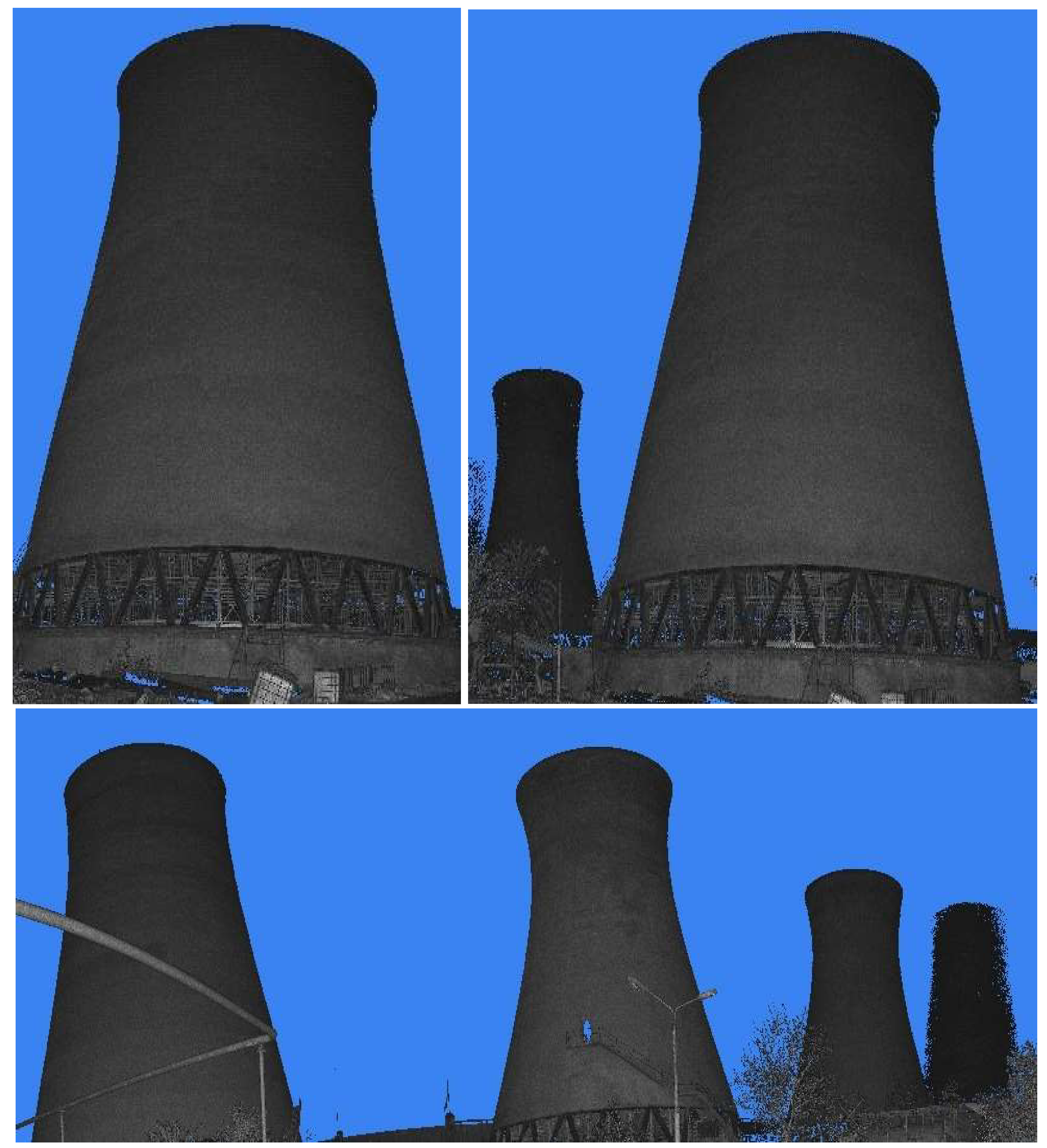
Figure 8.
Photo of the studied high rise cooling tower obtained from laser scanner.
Figure 8.
Photo of the studied high rise cooling tower obtained from laser scanner.
Figure 9.
Geometric dimensions of the studied four cooling towers resulted from geodetic observations.
Figure 9.
Geometric dimensions of the studied four cooling towers resulted from geodetic observations.
Figure 10.
The distribution of marks for testing TLS observations in deformation monitoring.
Figure 10.
The distribution of marks for testing TLS observations in deformation monitoring.
Figure 11.
Vertical sections for cooling tower No. 1 for determining the wall curvature type.
Figure 11.
Vertical sections for cooling tower No. 1 for determining the wall curvature type.
Figure 12.
Inclination of cooling tower axis in two directions.
Figure 12.
Inclination of cooling tower axis in two directions.
Figure 13.
Graphical representation of the studied high rise cooling tower walls deformation after projection on a vertical plane.
Figure 13.
Graphical representation of the studied high rise cooling tower walls deformation after projection on a vertical plane.
Figure 14.
Plan of the studied high rise cooling tower walls deformation.
Figure 14.
Plan of the studied high rise cooling tower walls deformation.
Table 1.
Geometric dimensions of the studied four cooling towers resulted from geodetic observations.
Table 1.
Geometric dimensions of the studied four cooling towers resulted from geodetic observations.
| | Base Diameter, m | Top Diameter, m | Tower Height, m |
|---|
| Cooling Tower No. 1 | 37.74 | 20.538 | 56.01 |
| Cooling Tower No. 2 | 28.28 | 16.08 | 39.475 |
| Cooling Tower No. 3 | 28.77 | 15.19 | 39.782 |
| Cooling Tower No. 4 | 37.71 | 21.21 | 55.971 |
Table 2.
Comparison of movement’s values resulted from TLS observations and vernier.
Table 2.
Comparison of movement’s values resulted from TLS observations and vernier.
| Movements Type | Distance | Proposed Movements, (mm) | Distance Measured by Vernier, (mm) | Calculated Distance from TLS Observations, (mm) | Difference of Distance between Vernier and TLS Observations, (mm) |
|---|
| Vertical movement | C-C/ | 110 | 110.44 | 111.81 | −1.37 |
| 85 | 84.46 | 85.75 | −1.29 |
| 60 | 60.52 | 61.86 | −1.34 |
| 35 | 35.48 | 36.95 | −1.47 |
| F-F/ | 30 | 29.84 | 31.65 | −1.81 |
| 20 | 19.28 | 17.49 | 1.79 |
| 18 | 18.52 | 19.84 | −1.32 |
| 15 | 15.06 | 16.67 | −1.61 |
| Horizontal Movements | D-D/ | 95 | 95.54 | 96.98 | −1.44 |
| 80 | 79.62 | 78.44 | 1.18 |
| 65 | 64.98 | 66.81 | −1.83 |
| 40 | 39.34 | 41.46 | −2.12 |
| E-E/ | 30 | 29.36 | 30.75 | −1.39 |
| 25 | 25.66 | 23.88 | 1.78 |
| 18 | 18.66 | 17.44 | 1.22 |
| 12 | 11.92 | 10.16 | 1.76 |
Table 3.
Calculated curve equation parameters for wall sections of cooling tower No. 1.
Table 3.
Calculated curve equation parameters for wall sections of cooling tower No. 1.
| Section | Curve Equation Parameters | Term
(B2 − 4AC) | Section Type |
|---|
| A | B | C | D | E | F |
|---|
| 1 | 0.3156 | 1.578 × 10⁻⁹ | 0.3156 | −269.7875 | −527.2805 | 277,858.2702 | −0.3984 | Circle |
| 2 | 0.0391 | 1.955 × 10⁻¹⁰ | 0.0391 | −33.4242 | −65.3253 | 34,424.1393 | −0.0061 | Circle |
| 3 | 0.1779 | 8.893 × 10⁻¹⁰ | 0.1779 | −152.0418 | −297.1550 | 156,590.2153 | −0.1265 | Circle |
| 4 | 0.0900 | 4.498 × 10⁻¹⁰ | 0.0900 | −76.9014 | −150.2983 | 79,201.9328 | −0.0324 | Circle |
| 5 | 0.2258 | 1.129 × 10⁻⁹ | 0.2258 | −193.0229 | −377.2495 | 198,797.2035 | −0.2039 | Circle |
| 6 | 0.0890 | 4.4485 × 10⁻¹⁰ | 0.0890 | −76.0551 | −148.6443 | 78,330.3241 | −0.0317 | Circle |
Table 4.
The adjusted values of several circular cross section radius and center coordinates from surface points coordinates resulted from TLS observations for cooling Tower No. 1.
Table 4.
The adjusted values of several circular cross section radius and center coordinates from surface points coordinates resulted from TLS observations for cooling Tower No. 1.
| Height of Cooling Tower Circular Cross Section above Ground, m | Calculated Radius of Each Circular Section of Cooling Tower Using Least Squaresand Its Accuracy | Calculated Circular Center Coordinates for Each Cross Section and Its Accuracy |
|---|
| ract., m | σr, mm | X, m | σX, mm | Y, m | σY, mm |
|---|
| 2 | 18.5761 | 2.2 | 67.2412 | 2.4 | 80.686 | 3.1 |
| 4 | 17.8496 | 2.1 | 67.2404 | 2.6 | 80.684 | 2.5 |
| 6 | 17.4272 | 2.8 | 67.2387 | 2.7 | 80.6828 | 2.8 |
| 8 | 16.9874 | 2.1 | 67.2383 | 1.9 | 80.6821 | 3.1 |
| 10 | 16.5068 | 1.9 | 67.2347 | 2.6 | 80.6777 | 3.2 |
| 12 | 16.1234 | 1.5 | 67.2366 | 3.1 | 80.6802 | 1.9 |
| 14 | 15.6825 | 1.6 | 67.2375 | 2.6 | 80.6813 | 2.8 |
| 16 | 15.1618 | 1.9 | 67.2397 | 2.7 | 80.6835 | 2.9 |
| 18 | 14.8068 | 2.1 | 67.2442 | 2.5 | 80.6819 | 3.1 |
| 20 | 14.4568 | 2.3 | 67.2475 | 1.9 | 80.6778 | 3.5 |
| 22 | 13.914 | 2.4 | 67.2464 | 3.0 | 80.6791 | 2.8 |
| 24 | 13.4947 | 1.5 | 67.2506 | 2.7 | 80.6979 | 2.9 |
| 26 | 12.7961 | 1.4 | 67.2521 | 1.5 | 80.7006 | 2.7 |
| 28 | 12.5458 | 1.2 | 67.2537 | 3.2 | 80.7019 | 1.9 |
| 30 | 12.4334 | 1.9 | 67.2508 | 3.1 | 80.6979 | 3.1 |
| 32 | 11.8673 | 2.3 | 67.2545 | 2.2 | 80.7032 | 3.4 |
| 34 | 11.6003 | 2.4 | 67.2626 | 2.3 | 80.7138 | 1.9 |
| 36 | 11.2891 | 1.7 | 67.2536 | 1.9 | 80.7019 | 2.5 |
| 38 | 11.16245 | 1.6 | 67.2507 | 2.5 | 80.6979 | 2.8 |
| 40 | 10.9242 | 1.8 | 67.2474 | 3.4 | 80.694 | 3.6 |
| 42 | 10.8542 | 0.9 | 67.2501 | 3.1 | 80.6979 | 2.1 |
| 44 | 10.6745 | 1.8 | 67.2493 | 2.8 | 80.6966 | 1.7 |
| 46 | 10.1684 | 1.9 | 67.2472 | 2.9 | 80.694 | 1.9 |
| 48 | 9.7667 | 2.1 | 67.2464 | 3.1 | 80.6926 | 3.2 |
| 50 | 9.6675 | 2.4 | 67.2395 | 1.6 | 80.6894 | 2.6 |
| 52 | 9.9295 | 1.7 | 67.2347 | 1.8 | 80.6978 | 2.8 |
| 54 | 10.1022 | 2.2 | 67.2339 | 2.2 | 80.6995 | 2.6 |
| 56.01 | 10.2688 | 2.1 | 67.2356 | 2.7 | 80.6961 | 2.9 |
| Max. | 18.5761 | 2.8 | 67.2622 | 3.4 | 80.7138 | 3.6 |
| Min. | 9.6675 | 0.9 | 67.2332 | 1.5 | 80.6777 | 1.7 |
| average | 13.1084839 | 1.92 | 67.2447 | 2.54 | 80.6918 | 2.73 |
| S.D. | 2.785341477 | 0.412182 | 0.007416 | 0.509331 | 0.009496 | 0.518277 |
Table 5.
The inclination values for cooling tower axis in two directions each 2 m tower height.
Table 5.
The inclination values for cooling tower axis in two directions each 2 m tower height.
| Height of Cooling Tower Circular Cross Section above Ground, m | Values of Tower Axis Inclinations in X, Y, mm |
|---|
| QX | QY | |
|---|
| 2 | 0.0 | 0.0 | 0.00 |
| 4 | −0.8 | −2.0 | 2.15 |
| 6 | −2.5 | −3.2 | 4.06 |
| 8 | −2.9 | −3.9 | 4.86 |
| 10 | −6.5 | −8.3 | 10.54 |
| 12 | −4.6 | −5.8 | 7.40 |
| 14 | −3.7 | −4.7 | 5.98 |
| 16 | −1.5 | −2.5 | 2.92 |
| 18 | 3.0 | −4.1 | 5.08 |
| 20 | 6.3 | −8.2 | 10.34 |
| 22 | 5.2 | −6.9 | 8.64 |
| 24 | 9.4 | 11.9 | 15.16 |
| 26 | 10.9 | 14.6 | 18.22 |
| 28 | 12.5 | 15.9 | 20.23 |
| 30 | 9.6 | 11.9 | 15.29 |
| 32 | 13.3 | 17.2 | 21.74 |
| 34 | 21.4 | 27.8 | 35.08 |
| 36 | 12.4 | 15.9 | 20.16 |
| 38 | 9.5 | 11.9 | 15.23 |
| 40 | 6.2 | 8.0 | 10.12 |
| 42 | 8.9 | 11.9 | 14.86 |
| 44 | 8.1 | 10.6 | 13.34 |
| 46 | 6.0 | 8.0 | 10.00 |
| 48 | 5.2 | 6.6 | 8.40 |
| 50 | −1.7 | 3.4 | 3.80 |
| 52 | −6.5 | 11.8 | 13.47 |
| 54 | −7.3 | 13.5 | 15.35 |
| 56.01 | −5.6 | 10.1 | 11.55 |
| Disclaimer/Publisher’s Note: The statements, opinions and data contained in all publications are solely those of the individual author(s) and contributor(s) and not of MDPI and/or the editor(s). MDPI and/or the editor(s) disclaim responsibility for any injury to people or property resulting from any ideas, methods, instructions or products referred to in the content. |
© 2023 by the authors. Licensee MDPI, Basel, Switzerland. This article is an open access article distributed under the terms and conditions of the Creative Commons Attribution (CC BY) license (https://creativecommons.org/licenses/by/4.0/).


