

Flow-Data-Based Global Spatial Autocorrelation Measurements for Evaluating Spatial Interactions
1
School of Architecture and Art, North China University of Technology, Rd.5 Jinyuanzhuang, Beijing 100144, China
2
School of Geographic Science, Nanjing Normal University, Nanjing 210023, China
*
Author to whom correspondence should be addressed.
ISPRS Int. J. Geo-Inf. 2023, 12(10), 396; https://doi.org/10.3390/ijgi12100396
Submission received: 31 May 2023
/
Revised: 31 August 2023
/
Accepted: 11 September 2023
/
Published: 28 September 2023
Abstract
:Spatial autocorrelation analysis is essential for understanding the distribution patterns of spatial flow data. Existing methods focus mainly on the origins and destinations of flow units and the relationships between them. These methods measure the autocorrelation of gravity or the positional and directional autocorrelations of flow units that are treated as objects. However, the intrinsic complexity of actual flow data necessitates the consideration of not only gravity, positional, and directional autocorrelations but also the autocorrelations of the variables of interest. This study proposes a global spatial autocorrelation method to measure the variables of interest of flow data. This method mainly consists of three steps. First, the proximity constraints of the origin and destination of a flow unit are defined to ensure similarity of flow units in terms of direction, distance, and position. This undertaking aims to determine the neighborhood of flow units and generate their adjacent matrices. Second, a spatial autocorrelation measurement model for flow data is constructed on the basis of the adjacent matrix generated. Artificial data sets are also employed to test the validity of the model. Finally, the proposed method is applied to the flow data analysis of population migration in central and eastern China to prove the practical application value of the model. The proposed method is universal and can be generalized to the global spatial autocorrelation analysis of any type of flow data.
1. Introduction
The identification of the spatial patterns of geographical events or phenomena is a fundamental topic in geographical research. Spatial autocorrelation measurement is one of the most common methods for quantifying spatial patterns. Spatial autocorrelation is defined as the nonrandom distribution of spatial variables on the basis of spatial location [1,2]. Spatial autocorrelation in GIS clarifies the degree to which one object is similar to other nearby objects. The First Law of Geography emphasizes the universality of spatial autocorrelation in space by explaining that everything is related to everything else, although near things are more related than distant things [3]. Given that spatial flow data receive considerable attention [4], the development of effective quantitative analysis models to measure the spatial autocorrelation of flows is significant for the spatial pattern analysis of flow data. Moreover, it could also expand the application scope and universality of spatial autocorrelation in GIS.
Although important progress has been made in the research of the spatial autocorrelation of OD flows, the complexity of OD flow data relative to traditional polygon data leads to multiple connotations for the spatial autocorrelation of OD flows [5]. The distinct data structure of OD flow data compared to traditional point and polygon data leads to many different perspectives on the measurement of the spatial autocorrelation of OD flows. For example, we can measure the spatial autocorrelation of the direction of flow data or the spatial autocorrelation of the relationship between outflow origins and inflow destinations [6,7]. We can also treat each OD flow unit as a whole and measure the spatial autocorrelation of a certain numerical attribute. This study focuses on the first case; that is, starting from the integrity of the flow unit and then discussing the global spatial autocorrelation of the flow attributes of the flow unit.
This paper is organized as follows: The literature of the spatial autocorrelation of OD flow data is reviewed in Section 2. In the specific research work part in Section 3, the possible basic types of OD flow units are introduced (Section 3.1), and the construction of the rules of proximity between flow units is further explained (Section 3.2). In the following section (Section 4), the extension of the traditional Moran’s I method proposed in this work to the spatial autocorrelation analysis of OD flow data is explored (Section 4.1). The effectiveness of the proposed method is subsequently verified (Section 4.2) through artificial data sets. Finally, on the basis of OD flow data of population migration in eastern China, the proposed method is used to conduct a case analysis to demonstrate the practical application value of the method in the analysis of spatial interaction problems; the analysis is discussed in Section 5. The discussion, conclusion, and future work are presented in Section 6. The proposed method can effectively analyze the spatial autocorrelation of OD flow data traffic or other numerical attributes from a global level. It can also quantify the overall trend of agglomeration, dispersion, or random distribution. The method enriches the understanding of the spatial distribution patterns of OD flow data.
2. Literature Review
Relevant research over the past few decades reveals that the spatial interactions of flow data are no longer a novel research topic. Studies on the measurement and interpretation of spatial interactions in flow data were already being undertaken as early as the 1970s [8,9,10]. Such early research opened the door to flow data studies. However, hardly any breakthrough was made because at the time, the volume of flow data was generally large and the computing capacity of computers was limited. Moreover, OD flow data were not as widely used as point and polygon data. Hence, scholars did not pay close attention to the topic.
In the subsequent period, flow data research from a geospatial perspective shifted focus towards the measurement, analysis, and visualization of interactions [11,12,13]. In addition, the research on the measurement of spatial autocorrelations in OD flow data gradually emerged [14,15]. However, research during this stage had yet to develop a systematic understanding of the measurement of spatial autocorrelations of flow data. Hence, Fotheringham [16,17] introduced flow data analysis on the basis of the gravity model [18] and explained the definition of spatial interaction in detail [19]. Models on spatially autocorrelated errors and spatial autoregressive errors and heterogeneity in OD flow analysis were later proposed and applied [20]. Anselin studied the application and spatial autocorrelation of flow data in econometrics, emphasizing the gravity and spatial autocorrelation measurement of flow interactions [21,22]. This pioneering research focused on developing spatial autocorrelation measurements for flow data via gravity models, with applications in economic geography.
In the 1990s, Getis introduced the conventional spatial autocorrelation analysis method, which can be applied to detect patterns in various types of data, including point data (quantitative data associated with discrete location coordinates), polygon data (data related to areal units and boundaries), and flow data (data that represent movements, interactions, or transportation between origins and destinations) [9]. Getis contended that the spatial interaction model is a special case of a spatial autocorrelation model and proposed a general statistic. Black proposed the concept of the autocorrelation of flow, which includes network autocorrelation and spatial autocorrelation for flow data [23]. Black believed that the autocorrelation that stresses the connectivity between nodes belongs to network autocorrelation, and that the autocorrelation that treats origins and destinations as objects belongs to spatial autocorrelation. In reality, Getis treated a flow unit as an object and emphasized the universality of the conventional spatial autocorrelation method in flow data analysis. Black’s categorization and precise definition of the spatial autocorrelation of flow data helped deepen people’s understanding of flow data. The primary contribution during that stage was a comprehensive understanding of the classification and definitions of spatial autocorrelation. However, there was no systematic study exploring the application of various existing spatial autocorrelation models to the two types of autocorrelation analysis for flow data.
With increasing understanding of spatial autocorrelation in flow data, more detailed and in-depth autocorrelation research on flow data has emerged. Representative studies include the fundamental theory of flow data spatial autocorrelation and the modifiable areal unit problem (MAUP) related to flow data origins and destinations [2,24,25]. Subsequently, the network autocorrelation model, spatial economic interaction autocorrelation, and regression model related to flow data were proposed and applied [26,27,28,29]. A number of conventional methods of autocorrelation measurement were also introduced into the network autocorrelation model [27,30,31,32]. New network autocorrelation models for flow data were later proposed, and new applications were extended accordingly; examples include the local autocorrelation model based on the difference-in-differences technique [33,34], spatial economic OD flow model [35,36], and Bayesian spatial interaction model [33].
These studies predominantly focused on autocorrelation in flow data. Moreover, most autocorrelation measurement models were developed based on flow values between origins and destinations, relying primarily on the Poisson distribution. In contrast, models following Black’s definition are chiefly network autocorrelation models, with only a limited number of studies exploring spatial autocorrelation specifically for flow data. The research related to spatial autocorrelation dates back to a series of studies on the spatial filtering of feature vectors [37,38] and its relevant application research [39,40,41]. Liu et al. introduced a general spatial autocorrelation analysis model for vectors, which reflect the general form of OD flow [6]. A notable feature of this study is that the direction of flow units was incorporated into the implementation logic of the model as part of the autocorrelation measurement.
Getis [8] contended that the common elements of various spatial autocorrelation models include (1) the matrix denoting the association among spatial elements (Condition 1: spatial weight matrix) and (2) the attribute values of spatial elements representing different positions (Condition 1: variable of interest). For conventional points and polygons, point or polygon objects are the spatial elements in Condition 1, and the values of variables used for spatial autocorrelation analysis are the attribute values in Condition 2. Similarly, when the object of analysis is flow data, the OD flow unit as a whole object represents the spatial element in Condition 1, and the flow value of the OD flow unit represents the attribute value in Condition 2. In accordance with this definition, the attributes of a flow unit are the variables of interest for spatial autocorrelation measurement instead of the directions of flow units as a variable for autocorrelation analysis. Griffith and Liu [6,37,38] proposed a new spatial interaction autocorrelation analysis model on the basis of the basic characteristics (directions of flow units) of flow. At this stage, no researcher has proposed any spatial autocorrelation model on the basis of Getis’ definition. Accordingly, the current study attempts to fill this gap.
On the basis of Black’s study, our research (1) divides the autocorrelation of flow data into network autocorrelation and spatial autocorrelation, (2) agrees with the general model of spatial autocorrelation defined by Getis, and (3) treats the OD flow unit as an object and spatial element to be analyzed. Moreover, this study determines the spatial proximity matrix of flow data by constraining the neighborhood of the origin and destination. Thereafter, the global spatial autocorrelation model of flow data is constructed on the basis of the conventional Global Moran’s I. This study also tests the effectiveness of the model through artificial data sets and performs empirical analysis by using population migration data. This empirical analysis proves the practical application value of the proposed method.
3. Definition of Flow Unit and Its Spatial Proximity
3.1. Types of Flow Unit
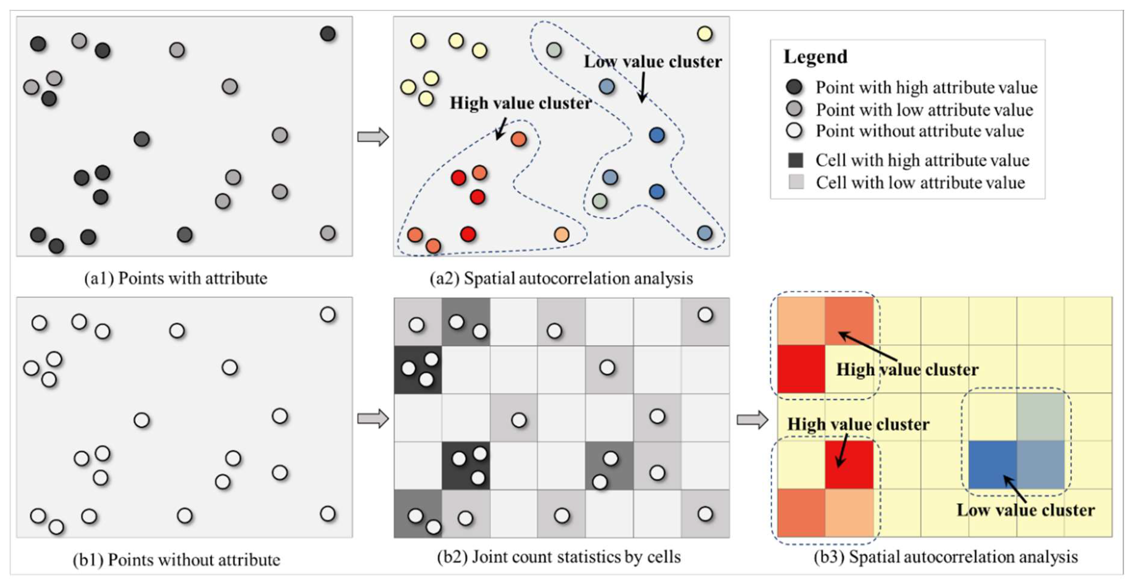
Spatial elements contain spatial and random information. In the spatial autocorrelation analysis, which is represented by Moran’s index and Geary C and et al. [42], the essence of measurement is to analyze the spatial association characteristics of a numeric interest variable of a geographic element. Such a numeric attribute belongs to non-spatial information. The spatial and geometric information of these geographic elements is mainly used to determine the spatial proximity and construction of the spatial proximity matrix. Accordingly, the following question should be answered: How can spatial autocorrelation be measured without a numerical variable for a set of points with spatial characteristics? The conventional methods are illustrated in Figure 1. Figure 1(a1) shows a set of spatial points. Different brightnesses represent different variable values; the darker the color, the larger the value, and vice versa. Specific information is provided in the legend. Given that this set of points has attribute information, global or local spatial autocorrelation can be measured using Moran’s I and other spatial autocorrelation analysis models.
The analysis result is shown in Figure 1(a2). However, spatial autocorrelation analysis cannot be performed directly for other cases, where a set of points may not contain any useful numerical variables. First, a common method is to divide the area where these points are located according to a certain geographic unit (e.g., administrative division, unit, or cell). Second, the number of points in each geographic unit is summarized by using sample statistics. Lastly, this statistic is used as the variable value for this geographic unit. The summary result of points in Figure 1(b1) is shown in Figure 1(b2). Evidently, the geographic units used for spatial autocorrelation analysis become polygons (cells), and the target variable for analysis becomes the number of points in each polygon. The analysis result is shown in Figure 1(b3). In this case, the basic geographic units used for spatial autocorrelation analysis are either points or polygons with numeric variable. Spatial autocorrelation analysis cannot be performed on points or polygons without numeric variable. This case provides the solution when the OD flow faces similar situations.
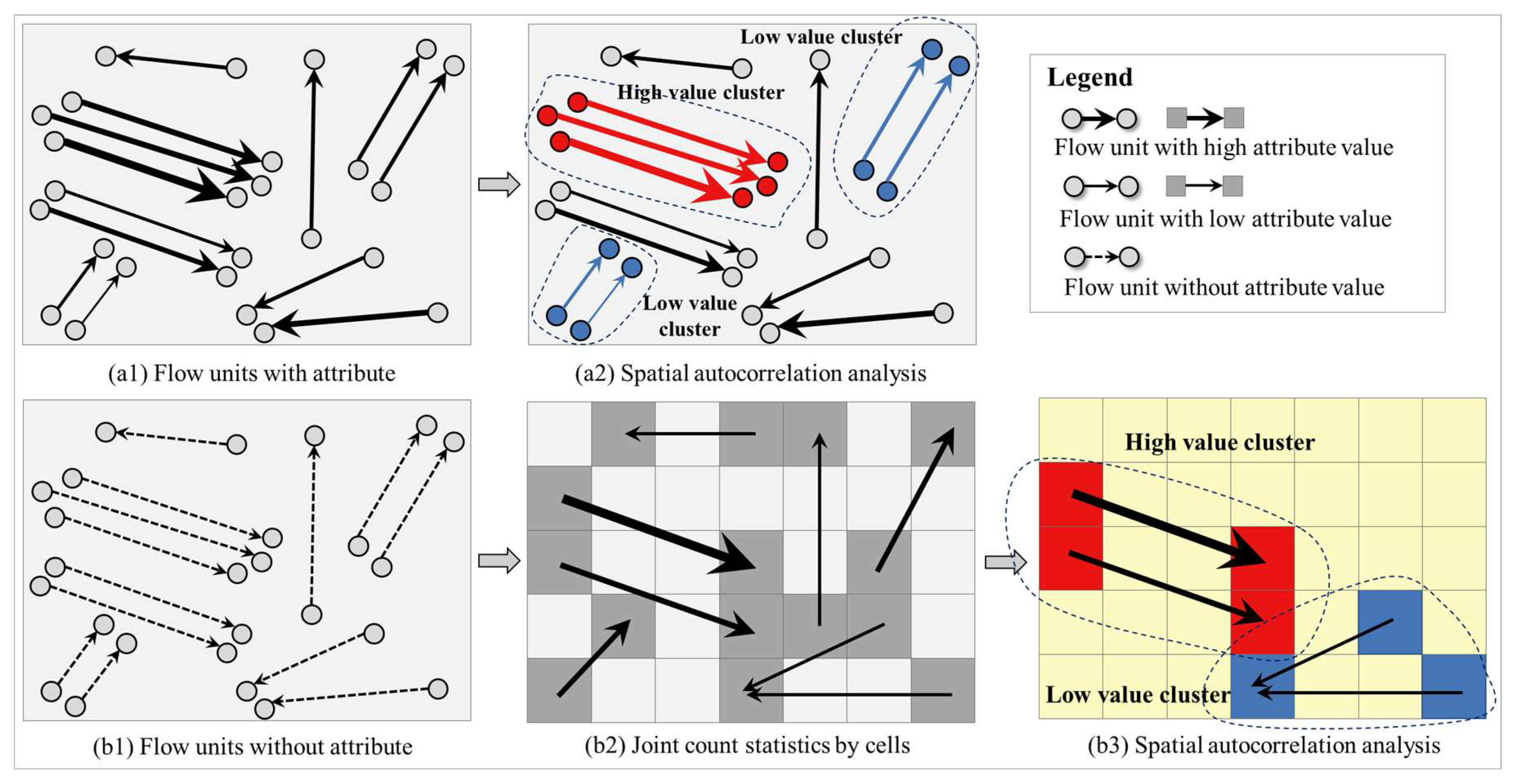
Unlike such elements as points and polygons, the basic units of the OD flow data generally comprise the origin, destination, and direction. The OD flow with numeric variables of interest consists of the origin, destination, direction, and variable. These two types of flow units form the basic structure of flow data. Figure 2(a1) shows the flow units with variables, where the thickness of the arrow indicates the size of the target variable. Figure 2(b1) shows the flow units without variables. Similar to point- or polygon-based spatial autocorrelation analysis, the analysis of the OD flow data should also be based on a numeric variable. Autocorrelation analysis cannot be performed directly for flow units without variables. Figure 2(a2) shows the autocorrelation analysis result of the flow units with variables. For the flow units without variables, a summary can be made on the basis of the polygon geographic unit, and the results can be concluded (see Figure 2(b2)). The thicker the arrows in Figure 2(b2), the greater the flow from the origin to the destination areas. At this time, the flow units without variables are converted into flow units with variables, with the variable being the flow value between the two areas. The flow value will be the target variable for spatial autocorrelation analysis. Figure 2(b3) shows the spatial autocorrelation result of flow data in the area shown in Figure 2(b2).
3.2. Spatial Proximity of the Flow Unit
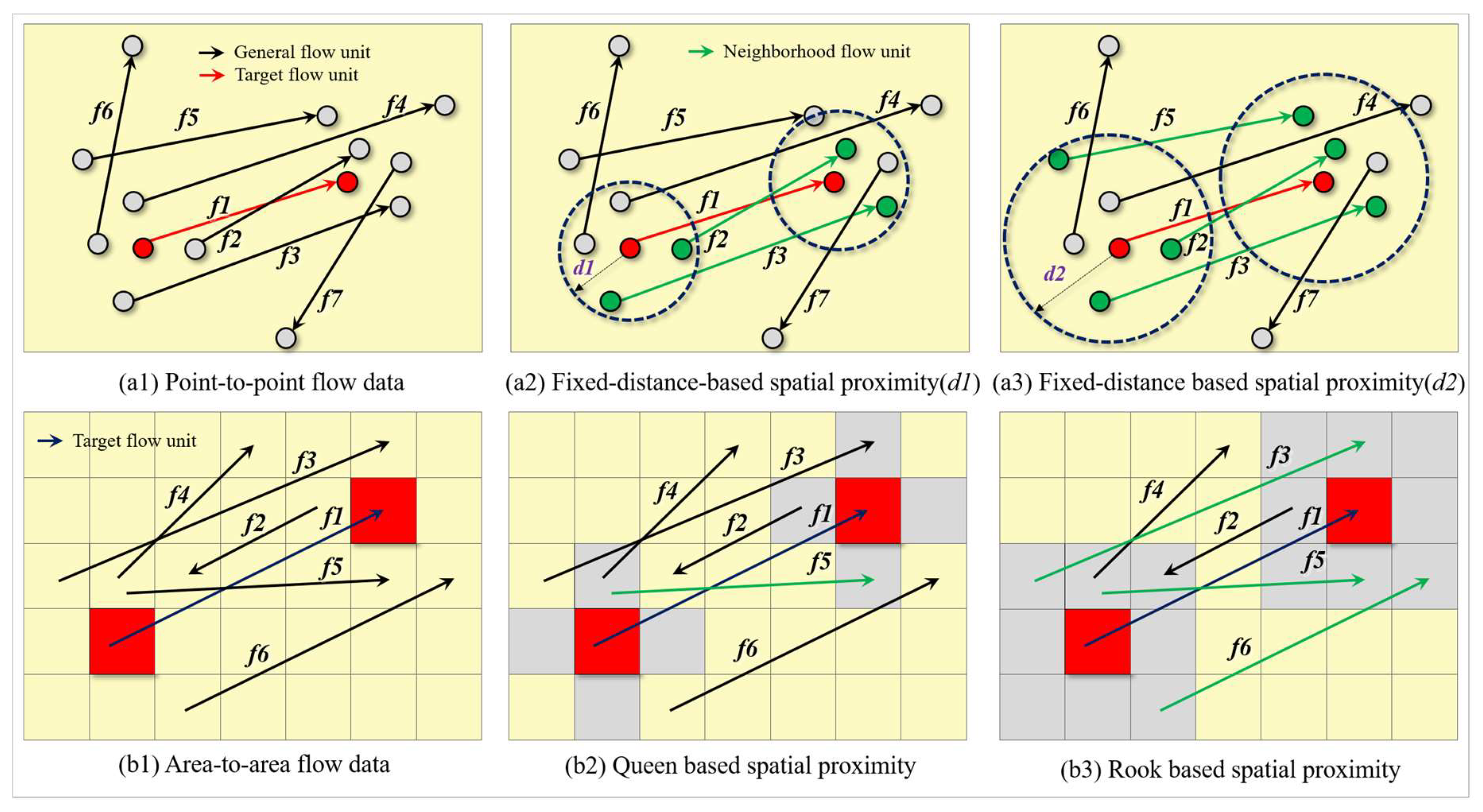
Before conducting spatial autocorrelation analysis, the spatial proximity rule among elements must be determined, and spatial proximity matrices should be constructed on the bases of these rules. The spatial autocorrelation analysis of flow data is no exception. Spatial proximity between two flow units can be defined as follows: For two origin-destination (OD) flow units and , if their respective origin locations are spatially proximate and their respective destination locations are also spatially proximate, then and can be considered spatially adjacent. This conceptualization, predicated on the inherent spatial properties of linked origin and destination points, constitutes a fundamental formulation of a spatial neighborhood between OD flow units. For example, Queen and Rook cannot be directly applied to point-based flow units, although they can be directly applied to area-based flow units. Thereafter, this study shows how to determine the spatial proximity of point- and area-based flow units through fixed-distance and the Queen-and-Rook rule, respectively.
Figure 3(a1) shows the point-to-point flow data with numerical variables. Figure 3(b1) shows the area-to-area flow data with numerical variables. Some rules for determining the proximity between flow units are generic and can be applied to any of the flow units (e.g., fixed-distance and k-nearest). By contrast, other rules can only be applied to area-to-area flow data (e.g., topology-based Queen and Rook). Other more complex neighborhood distance modeling methods include inverse distance and inverse distance squared et al. For flow unit f1 in Figure 3a, if fixed-distance is adopted as a rule and the neighborhood distance is set as d1, then the neighborhood distance of f1’s origin and destination can be determined (see Figure 3(a2)). Only f2 and f3’s origin and destination are within the neighborhood distance of f1. Therefore, only f2 and f3 are the neighbor units of f1. After extending the length from d1 to d2, the result is shown in Figure 3(a3), which suggests that in addition to f2 and f3, the origin and destination of f5 also fall in the neighborhood distance of f1. By this time, the neighbor flow units of unit f1 include f2, f3, and f5.
Figure 3(b1) indicates the area-to-area flow units. If f1 is considered the target flow unit and the Queen rule is the proximity rule, then the result of the neighbor units of f1 is shown in Figure 3(b2). This outcome suggests that only f5’s origin and destination area fall in the area that has a shared side with f1’s origin and destination (Queen rule). Thus, only f5 is the neighbor flow unit of f1. When adopting the Rook rule, the result is shown in Figure 3(b3). For the origin and destination areas of the target flow unit, only areas with a shared side or shared node are considered neighbor areas. In this instance, the neighbor flow units of f1 include f3, f5, and f6. Similar to points or polygons, the spatial autocorrelation effects of the flow units can be measured on the bases of the target variables once the spatial proximity matrix is determined.
4. Modeling Global Spatial Autocorrelation of Flow
4.1. Measuring Global Moran’s Index of OD Flow
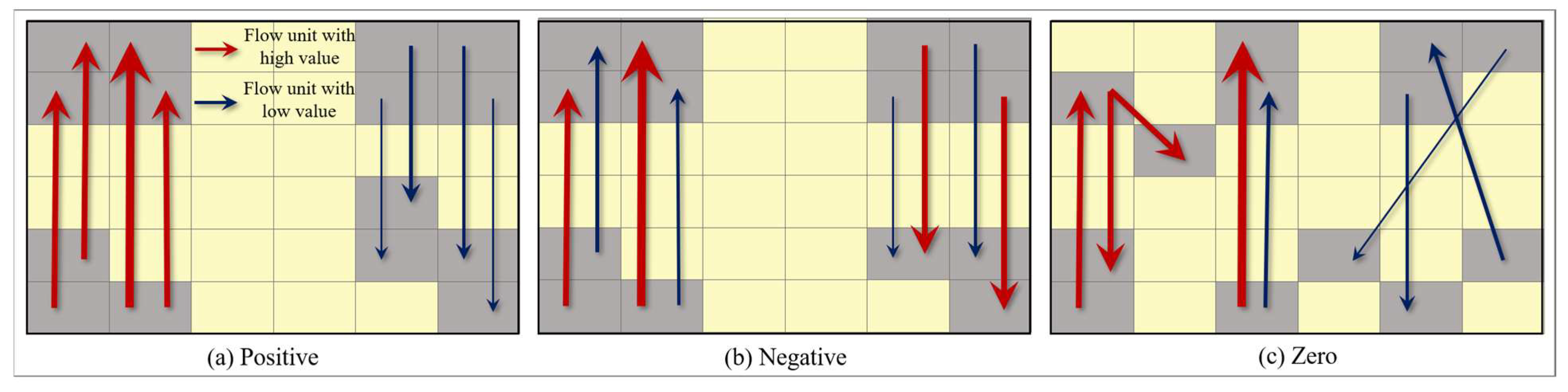
Three types of OD flow patterns are shown in Figure 4; the thicker the arrow, the higher the value of the interest variable and vice versa. In Figure 4a, each group of OD that flows with a similar position also has similar values of interest variables. For example, the interest variable values of the OD flows on the left are higher. Accordingly, this pattern is defined as a positive spatial autocorrelation. In Figure 4b, the interest variables of each group of OD flows have high and low values. Thus, no similarity exists. This type of pattern, in which a group of nearby flow units remain dissimilar, is defined as a negative spatial autocorrelation. The OD flows in Figure 4c exhibit a random distribution regardless of the spatial distribution or value of the interest variable. Thus, no spatial autocorrelation exists, which is defined as zero spatial autocorrelation. Thereafter, we will show how to measure whether these patterns have a spatial autocorrelation and what kind of spatial autocorrelation they belong to if there is spatial autocorrelation.
Moran’s I is one of the most widely used among a wide range of methods for measuring global spatial autocorrelation. If I denotes the global Moran’s index, then the equation of this index is as follows:
where denotes the spatial proximity between flow unit i and j. If we assume the flow units i and j are spatially proximate, then ; otherwise, ; and , where and denote the attribute values of flow units i and j, respectively. If we assume that n denotes the total number of flow units, then indicates the average attribute value of the n flow units. The equation of is as follows:
Hence, the equation for the Global Moran’s I can be specifically expressed as follows:
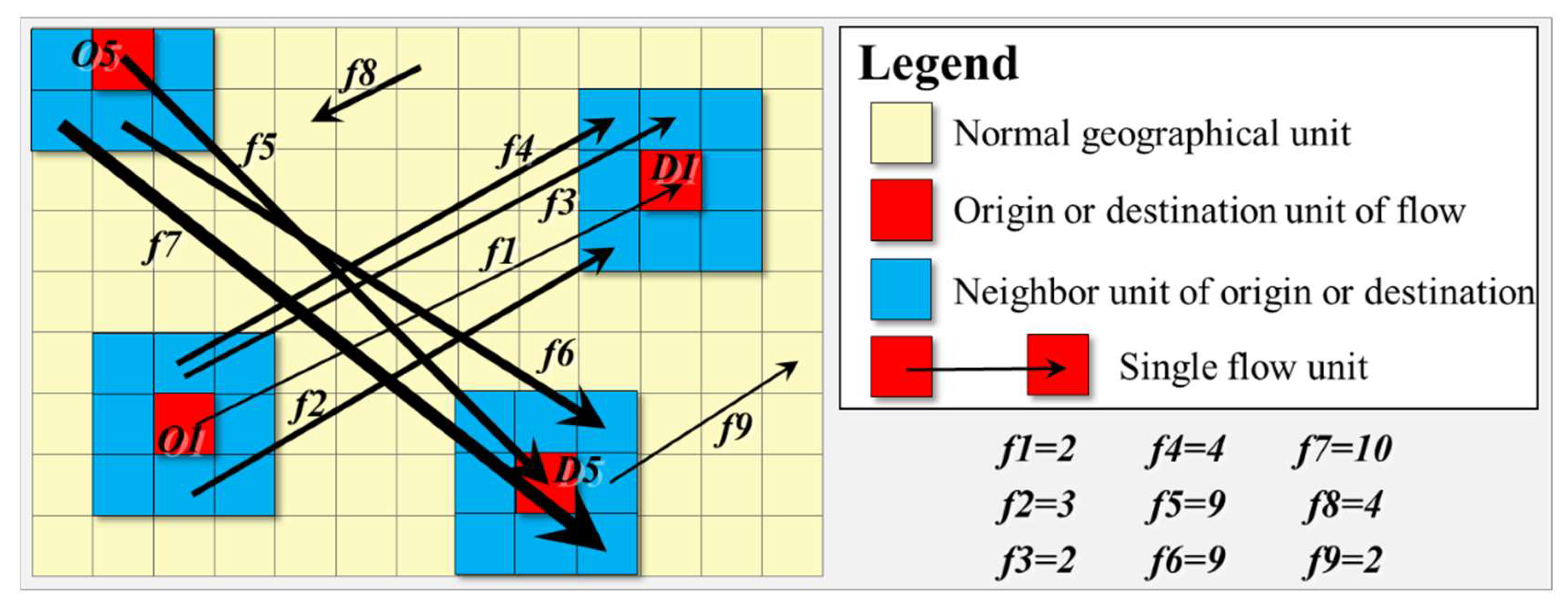
To understand this equation, we use Figure 5 to demonstrate the calculation process. Figure 5 contains nine flow units, with the directions and thickness of arrows indicating the directions and sizes of flows, respectively. Evidently, flow units f1, f2, f3, and f4 have similar origin and destination areas, and their flow values are low, thereby forming clusters with low flow values. Flow units f5, f6, and f7 have similar origin and destination areas and their flow values are high, thereby forming clusters with high flow values. Apart from these units, some discrete flow units exist, such as f8 and f9. The legend indicates the flow value of each flow unit. Therefore, n = 9, which is the total number of flow units. The equation of the average value = 5 and .
For flow unit f1, we can obtain the neighbor area of the origin area O1 and destination area D1 on the basis of the definition of proximity and by using the Rook rule. OSet1 denotes the set of the neighbor area of O1, and DSet1 denotes the set of the neighbor area of D1. For any flow unit fi, if the origin area of flow unit fi and the destination area of flow unit fi , then fi is a neighbor flow unit of f1. This method indicates that the neighbor flow units of f1 are f2, f3, and f4. Similarly, the neighbor flow units of f5 are f6 and f7 (see Table 1).
On the basis of the data in Table 1, the partial result of , when i = 1 and i = 5, can be obtained as follows:
This calculation method is used and each flow unit is taken as target. Moreover, the neighbor flow units of the target flow unit are sought, thereby yielding the following result:
Given that Rook is adopted as the proximity rule in this case, when the flow and target flow units are spatially proximate, ; otherwise, . Thus, the value of is the sum of the neighbor units of each flow unit:
Global Moran’s I can be calculated as follows after obtaining all the variables needed:
Obtaining Global Moran’s I is merely the first step in measuring global spatial autocorrelation. Additional testing is required to determine whether the observed value of Moran’s I significantly deviates from randomness. We should conduct tests and calculations on the bases of the expected or mean value of Global Moran’s I and its standard deviation. The Z-Score can be typically used to test such a significance. The Z-Score equation is as follows:
where I is the observed value, is its expected value, and is the standard deviation of Global Moran’s I. The equation of is as follows:
Therefore, the more flow units are evaluated (i.e., the higher the value of n), the expected value of Global Moran’s I approaches 0. Under random assumptions, the standard deviation equation for Global Moran’s I is as follows:
On the basis of this equation, the Z-Score of the example (see Figure 2) can be obtained. Moreover, whether the OD flow is distributed in a clustered manner, discretely, or randomly, can also be determined. The significance level of the spatial autocorrelation can also be obtained. When Z is above 2.58, the flow data in the study area is distributed in aggregation with high or low flow values at a 99% confidence interval. When Z is between 1.96 and 2.58, the flow data in the study area exhibits a clustered distribution with high or low flow values at a 95% confidence interval.
When Z is between 1.65 and 1.96, the flow data in the study area exhibit a clustered distribution in high or low flow values at a 90% confidence interval. This significance indicates that the flow value in the study area presents a positive spatial autocorrelation. In contrast, when Z falls in intervals of under −2.58, −2.58 to −1.96, or −1.96 to −1.65, the flow value of the flow data in the study area shows discrete distributions at the 99%, 95%, and 90% confidence intervals, respectively. This negative significance indicates that the flow in the study area presents a negative spatial autocorrelation. When Z is between −196 and 1.96, the null hypothesis cannot be rejected, thereby indicating that the flow in the study area is randomly distributed in space. The Z-Score of the flow data in Figure 2 is as follows:
The calculation result of Z is 3.031, meets , and the probability of the aggregation mode occurring randomly is below 1%, thereby indicating that the flow of the flow data in Figure 2 has a significant positive spatial autocorrelation. That is, the clustered distribution has high or low values at the 99% confidence interval.
4.2. Evaluation Efficiency of Model by Artificial Data Set
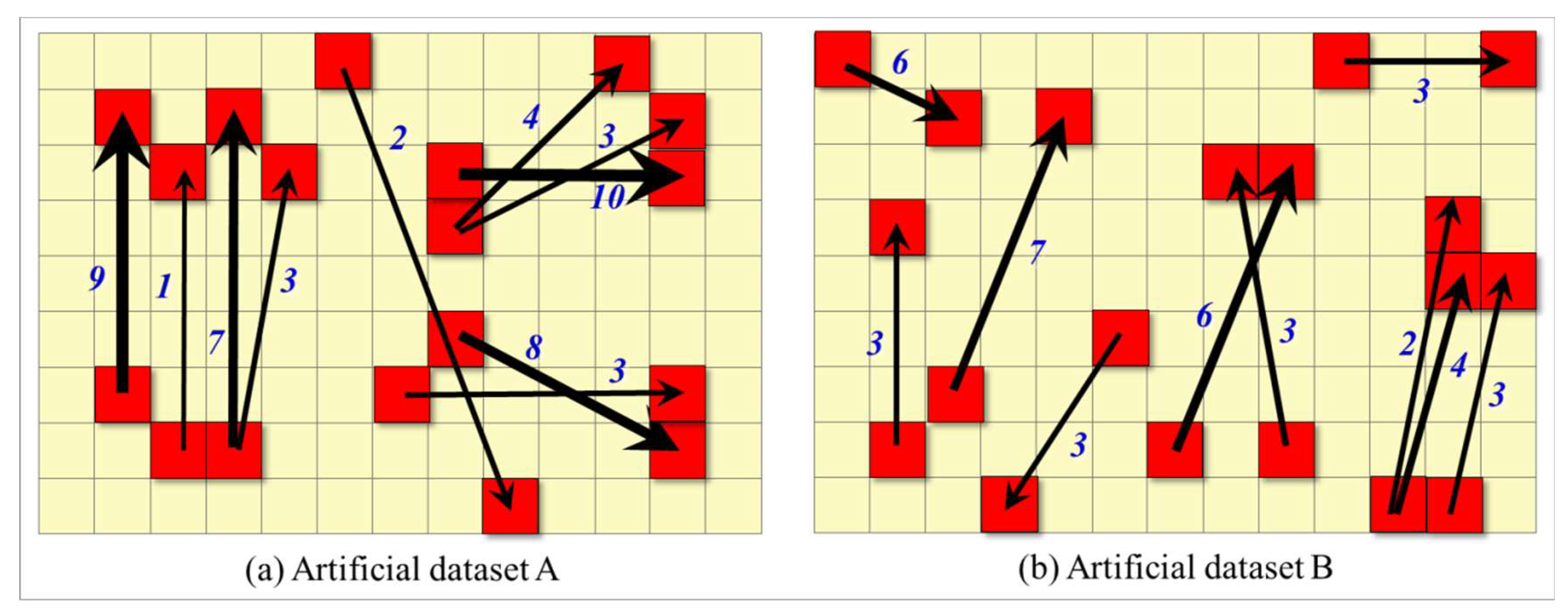
The flow data in Figure 5 contains unit clusters with high and low flow values. Moreover, the flow units with agglomeration characteristics account for a large proportion of the total number of all flow units. This result suggests that the flow units in this data set show significant characteristics of global aggregation (i.e., positive spatial autocorrelation). The purpose of elaborating the calculation of Global Moran’s I in Figure 5 is to illustrate how to measure the global spatial autocorrelation of the flow data. To verify the rationality and effectiveness of the method, two artificial data sets with clear objectives are employed (see Figure 6). The flow data in Figure 6a shows evident discrete distribution. In the first group of clustered flow units, the flow units with high and low flow values appear alternately, the clustered flow units of the second and third group show similar characteristics as the first group, and the flow units in the three groups account for the majority of the total units. That is, the flow values of the flow data in Figure 6a present global discrete distribution (i.e., negative spatial autocorrelation). In the flow data set shown in Figure 6b, the majority of the flow units appear to be randomly distributed, even for neighbor flow units, and the flow values are randomly distributed. Given that the majority of the flow units in Figure 6b are randomly distributed, the expectation is that the flow data lack global spatial autocorrelation features. To verify the validity of the proposed method, global spatial autocorrelation measurement is also performed on the flow data (see Figure 6a,b) using the method based on the Rook rule.
Table 2 shows the analysis results through calculation. The Moran’s I of artificial data set A is −0.761, and the Z-Score is −1.874, which meets . This result reveals that the probability of the random occurrence of the flow data pattern in artificial data set A is below 10%. Thus, the null hypothesis can be rejected. A significant negative spatial autocorrelation (i.e., discrete distribution) can be observed. The Moran’s I of artificial data set B is 0.256, and the Z-Score is 0.870, which meets . This result means that the flow data in artificial data set B cannot reject the null hypothesis and are randomly distributed. The calculation of Global Moran’s I and Z-Score test result are completely the same as expected. This result proves the effectiveness of measuring the OD flow data global spatial autocorrelation using the proposed method.
5. Application
5.1. Study Area and Data Description
This study uses eight adjacent provinces and one municipality in Southern China as study areas, utilizes the population flow data recorded in the highway system in 2018 as the data source, and demonstrates the measurement of the global spatial autocorrelation of population flow by using the proposed method. The dataset used in this paper comes from Tencent Migration Big Data, which is China’s largest Internet company and holds the country’s largest user base of online social platforms. The raw data provides records of migratory OD flows between different prefecture-level cities in China.
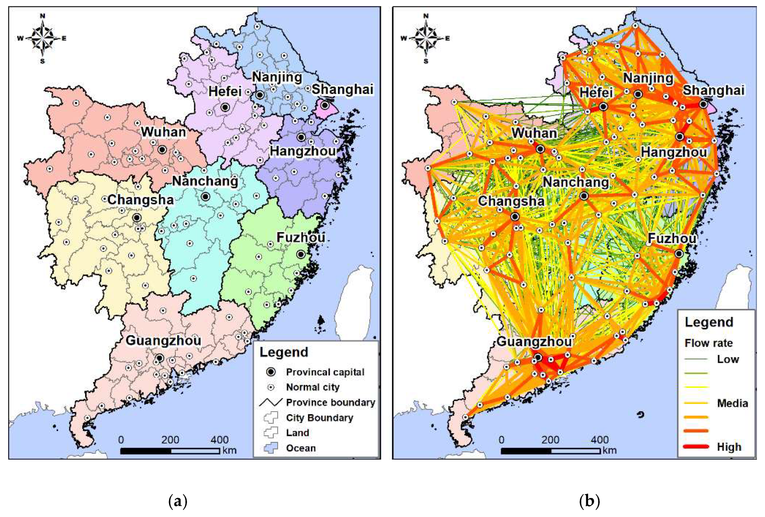
The study area shown in Figure 7a comprises three city clusters: (1) a cluster of central cities with Wuhan as the center, located in the middle reaches of the Yangtze River; (2) the Yangtze River Delta city cluster with Shanghai as the center; and (3) the Pearl River Delta city cluster with Guangzhou as the center. Most of these provinces and municipalities, which feature large populations, population migration, and facilitated transportation are located in China’s highly developed regions. The research data come from Tencent’s population migration data interface, which records the number of people entering and exiting each city through roads and highways every day. The data flow involves approximately 110 cities, with over 600,000 data flow entries throughout the year. Each data set contains the names, latitudes, and longitudes of the outflow and inflow cities, as well as the total flow population. These details constitute a complete flow unit. The summary of the flow data in 2018 is shown in Figure 7b.
Each flow data can be represented by , where and denote the size of the population moving in and out of the city, respectively, and VAL is the population that flows from city to city . Prior to the global spatial autocorrelation analysis, we need to construct a spatial proximity matrix for each flow unit. This study adopts the Queen rule, which specifies that the city that has a shared side or node with the target city, and is the neighbor unit of the target city. For flow unit , if the set of neighbor cities of origin area is the , then the set of neighbor cities of destination area is . For any flow unit , if and , then flow unit is the neighbor unit of flow unit . Similarly, if the neighbor unit of any flow unit can be identified in this manner, then global spatial autocorrelation measurement can be performed. Accordingly, population flow can be analyzed regardless of whether it is in aggregation, discrete, or in a random distribution. In this study, flow units are divided by month according to the time of occurrence. Eventually, the flow data subset at the summary level is obtained monthly for 12 months. Under the condition of a random hypothesis, the global spatial autocorrelation index is calculated using the proposed method, and its significance is tested using the z-score. The spatial aggregation degrees of the flow values across 12 months are then compared, and the variation rules are discussed.
5.2. Result
A city with a developed economy may drive the economic development of its surrounding cities. In addition, neighboring cities generally have similar location advantages, such as regional resource endowment and a sound geographical environment, which are also important for the aggregation of cities with developed economies. By contrast, a city with a less developed economy, possibly as a result of insufficient regional advantages or the absence of any effects from developed cities, may also present an aggregated distribution. The urban agglomeration effects on the development potential of an area outweigh all other aspects. A crucial driver behind population migration is the imbalance between supply and demand between two areas. Given that neighboring areas tend to be similar in terms of industry and economy, the areas where population flows out are generally the areas where labor-exporting cities agglomerate. These cities have sluggish industrial development and offer only a few jobs. By contrast, the areas where population flows in tend to be areas where cities with a shortage of labor agglomerate. These cities have many jobs to offer and develop rapidly. Verifying the significance of this trend is one of objectives of the proposed spatial autocorrelation method. The global spatial autocorrelation of population migration in 2018 in the study area is analyzed by month. The analysis results are presented in Table 3.
Table 3 lists the Moran’s I, expected index, standard deviation, and z-score each month. Moreover, Table 3 shows that in 12 months, all Moran’s I values are between 0 and 1, and all z-scores are above 2.58. These results suggest that the population migration for all months shows an aggregation distribution at the 99% confidence interval and general relative stability. The observation is that most of the z values are between 60 and 70, and that all Moran’s I values are between 0.3 and 0.4. The expected index and standard deviation are also within a certain threshold.
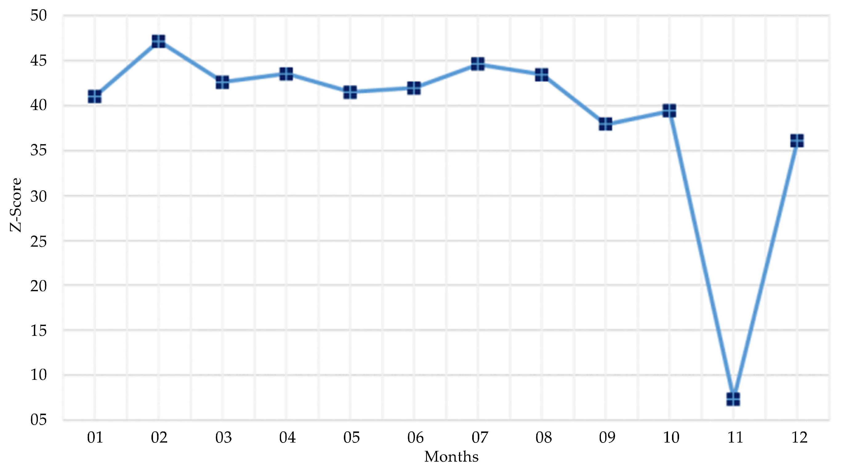
To observe the spatial autocorrelation of the population migration in different months and its evolution, we use month as the x-axis and Global Moran’s I as the y-axis in constructing the graph (Figure 8). Despite the general stability of the z-scores, the score in February (i.e., 80.863) is evidently higher than those of the other months. The z-score in November (i.e., 62.161) is the lowest. This result shows the evident spatial aggregation characteristics of population migration in the study area in February and November relative to those in the other months. The salient significant Moran’s I value observed globally in February is indicative of distinct spatial cluster patterns. While the predominant role of high or low clustering remains equivocal in February, such spatial autocorrelations generally arise from the collective influence of both high and low value clusters across most contexts.
On the basis of the full sample data, we extract all the flow data whose flow rate threshold is above 10,000 for each flow unit. With the same method, only the data that meet the threshold are analyzed. The analysis result is shown in Figure 9. Figure 9 shows that relative to that of the full sample flow data, the z-score of the subsample flow data is generally reduced from approximately 65 to approximately 40. The score for February remains higher than those of the other months, but with minimal fluctuation. The score for November shows the same tendency as the full sample. That is, the z-score is lower than the average value with substantial fluctuation. The z-score of November is far lower than the values of the other months.
Through the two-level analysis, and regardless of the use of full sample flow data or flow data with high flow values (except for February and November), we find that the other months present a relatively stable agglomeration effect at a 99% confidence interval, with the agglomeration degree showing minimal differences. Only the agglomeration degree of the flow data with a high flow threshold is less than that of the flow data of the full sample. Apart from having effectively detected the global aggregation mode, which is evidently different, this application also reveals an interesting fact: in the analysis results of the two flow data sets, the z-scores are considerably higher than 2.58, which is the threshold for the 99% significance level. This outcome is due to the huge difference in the total population flowing in and out of different cities every month. For cities with a large potential for population migration, the migration flow can reach 7 million per month. In contrast, for cities with minimal migration, the number may be only a few thousand or even just hundreds. Note that the data used in this study, which are obtained from the monitoring and sampling of location-based services, are not a full sample, and are thus not completely consistent with actual migration. Nonetheless, they are consistent in terms of proportion.
6. Discussion and Conclusions
6.1. Discussion
Given that flow data have various forms, the flow data that can be applied to spatial autocorrelation analysis using the proposed method are worth discussing [43]. Flow data have been widely applied, and the OD pair is among the most important forms, and can be referred to as OD flow. This particular flow data emphasizes the associations and interactions among different places or regions. In reality, taxi passengers getting on and off, subway passengers entering and exiting stations, capital flowing in and out, two places communicating, and tourists traveling from one country to another can all be abstracted as OD flow. Despite the extensive sources of OD, all flows can still be divided into two basic forms; namely, OD flow without numerical variables (e.g., origin and destination formed when taxi passengers get on and off) and OD flow with numerical variables (e.g., traffic data between two subway stations during a specific time period and population migration data between two cities). The former must be aggregated on the basis of geographic units or cells, and the flow data or other attributes between two areas after the aggregation must be used as the new numerical variable of the OD flow to meet the requirements of the proposed method. Therefore, with proper treatment, any OD flow can be analyzed using the proposed method.
Focus should be directed toward the construction of a spatial proximity matrix during the spatial autocorrelation analysis of flow data. Similar to the construction of a proximity matrix of points and polygons, the proximity matrix of flow data is also realized through topological proximity rules (e.g., Queen or Rook), number-based rules (e.g., K-nearest), and distance-based rules (e.g., inverse–distance or sequence–distance). Given that flow data must consider the proximity of the origin and destination, some special scenarios should also be considered aside from these constraints. For example, when using the K-nearest constraint, K = 8 is assumed, and it indicates eight neighbor origins of the origin of the target flow unit. However, the corresponding destinations are not necessarily the neighbor destinations of the target flow unit. In the extreme case, none of them are neighbor destinations. Thus, the issue in modeling the spatial proximity matrix is whether K-nearest should directly adopt this rule, or whether K = 8 should be defined as the nearest eight flow units of the target flow unit. In accordance with the definition of spatial autocorrelation, if the autocorrelation in the direction of the neighbor flow unit is considered, then the former should be adopted instead of the latter.
A spatial autocorrelation significance test should be conducted on the basis of random or standard normal distribution hypotheses. In the application analysis, the z-scores of the global spatial autocorrelations of two flow data sets are extremely high (i.e., above the 2.58 threshold), at the 99% confidence interval. The reason is similar to that of the high z-score of the spatial autocorrelation of a point or polygon. When the difference between the values of the analysis variables is huge, clusters with significantly high and low values are likely to occur. Given the z-score equation, the score is bound to be high. The huge difference in the flow values of the different flow units in the examples in this study is undoubtedly the main factor behind the high z-score.
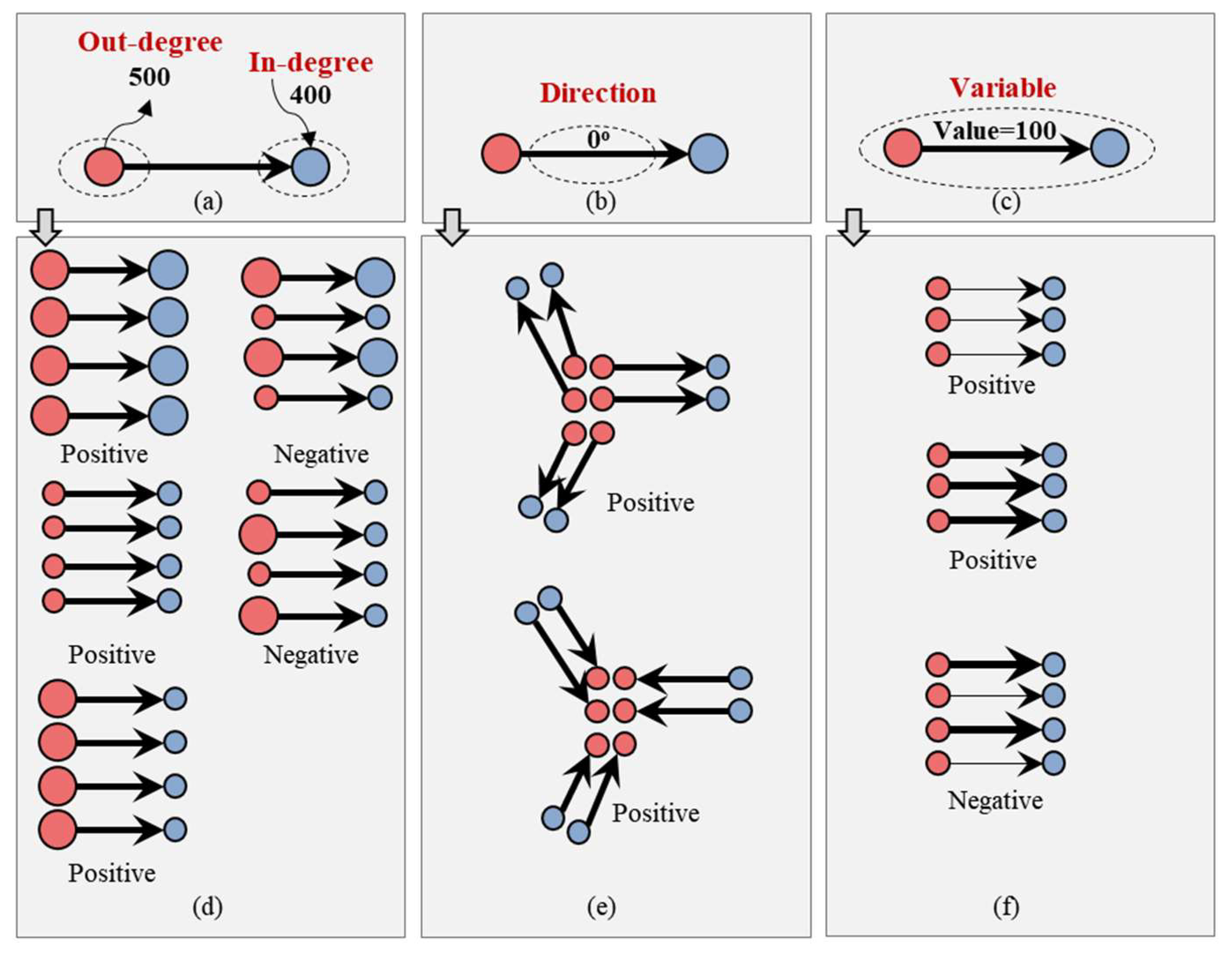
As we have previously emphasized, the data structure from the traditional point and polygon to the OD flow becomes increasingly complicated. For a flow unit, it is composed of the origin, destination, direction, and variable of interest. The target of measuring spatial autocorrelation can be one or more of these variables. Figure 10 shows examples of the spatial autocorrelation analysis of OD flow data from three different perspectives. In Figure 10a, for a group of flow units with adjacent relations, the concern is whether the out-degree and in-degree of each flow unit belongs to the same type. For example, the out-degree and in-degree could be either extremely large or small; that is, the out-degree is large, and the in-degree is small, or vice versa. Following this classification can facilitate the quantification of whether the distribution of OD flow has a spatial autocorrelation and help determine the type of spatial autocorrelation to which it belongs (Figure 10d).
In addition, the measurement of spatial autocorrelation can be shifted toward the direction of OD flow [6], as shown in Figure 10b. At this point, one could measure and determine the spatial autocorrelation mode and type shown in Figure 10e in the OD flow data. As shown in Figure 10c, the spatial autocorrelation measurement with the interest variable as the target is also a major direction. The interest variable can be any attribute value that needs to be analyzed, such as the flow of people, material flow, information flow, and capital flow. This research is also based on the perspective of constructing a global spatial autocorrelation model of OD flow, and attempts to evaluate whether the pattern shown in Figure 10f exists. The characteristic of OD flow with a composite structure indicates that the above situation must be considered when modeling spatial autocorrelation. In addition, a spatial autocorrelation measure based on multilayer networks distinguishes the three perspectives presented in Figure 10 [7].
6.2. Conclusion and Future Directions
By determining the spatial proximity elements of the origins and destinations of target flow units, the global spatial autocorrelation analysis method proposed in this study ensures the existence of neighbor origins and destinations between target flow units and their neighbor flow units. Moreover, the current research ensures that these flow units have similar lengths and directions. The construction of the spatial proximity matrix of OD flow is effective and meets the analysis requirements of global spatial autocorrelation. On the basis of the spatial proximity matrix of OD flow, and by adopting Global Moran’s I, this study effectively measures the global spatial autocorrelation of OD flow data. This process serves to enrich existing measurement methods and extend the application of Global Moran’s I in GIS.
In terms of effectiveness evaluation, negative spatial autocorrelation (discrete distribution) and nonspatial autocorrelation (random distribution) artificial data sets were designed (Section 3.2). In addition, the global spatial autocorrelation of two artificial data sets was measured using the proposed method. The analysis results are consistent with the designed goal and thus verifies the effectiveness of the proposed method. In terms of the application value, this study takes the OD flow data of population migration through highways and roads in the central and eastern regions of China in 2018 as the main data source. Global spatial autocorrelation analysis is also conducted on full sample data and the extracted subset of migration flow above 10,000 persons among cities. The analysis reveals that the two data sets show relative stability in 12 months, but that the degree of aggregation is high in February and low in November. The analysis successfully detects the global spatial autocorrelation effects of population migration across different months and its trend over time. The analysis also determines the months when abnormal global autocorrelation takes place. This finding is of immense value in understanding the overall spatial patterns of population migration.
Although this study has successfully proposed a global spatial autocorrelation analysis model for OD flow data based on Global Moran’s I, Global Moran’s I can only determine whether a set of flow data has a discrete, random, or aggregated distribution; it cannot establish whether the aggregation is of high or low value. Subsequent research will compensate for this deficiency by using G-statistics and other methods. In addition, global spatial autocorrelation can only measure the global tendency. Future research should be able to measure local spatial autocorrelation. In terms of result visualization, the local spatial autocorrelation of OD flow, which is different from that of conventional point and polygon data, requires a new visualized strategy and plan, which remains a considerable challenge. As far as this case study is concerned, it might be interesting, and important findings could be obtained if the streaming data used could distinguish between different types of population flows and if we could analyze how the highs and lows of the spatial autocorrelation of the different types of flows are clustered. This will be additional important work for us in the future.
Author Contributions
Conceptualization, Shuai Sun; Methodology, Haiping Zhang; Validation, Shuai Sun; Formal analysis, Haiping Zhang; Resources, Shuai Sun; Writing—original draft, Haiping Zhang; Writing—review and editing, Shuai Sun; Visualization, Haiping Zhang. All authors have read and agreed to the published version of the manuscript.
Funding
This research was funded by Beijing Municipal Social Science Foundation (22GLC062) and Beijing Municipal Education Commission Social Science Project (KM202010009002).
Data Availability Statement
A source code with C# language, artificial data, real-world experimental data, and software that we have we developed are available in GitHub (https://github.com/gissuifeng/Global-Autocorelation-of-OD-Flow), accessed on 10 September 2023.
Conflicts of Interest
The authors declare no conflict of interest.
References
- Anselin, L. Local indicators of spatial association—LISA. Geogr. Anal. 1995, 27, 93–115. [Google Scholar] [CrossRef]
- Griffith, D.A.; Paelinck, J.H.; Griffith, D.A.; Paelinck, J.H. Spatial Autocorrelation and the p-Median Problem. Morphisms Quant. Spat. Anal. 2018, 51, 9–24. [Google Scholar]
- Tobler, W.R. A computer movie simulating urban growth in the Detroit region. Econ. Geogr. 1970, 46, 234–240. [Google Scholar] [CrossRef]
- Andris, C.; Liu, X.; Ferreira, J. Challenges for social flows. Comput. Environ. Urban Syst. 2018, 70, 197–207. [Google Scholar] [CrossRef]
- Griffith, D.A.; Chun, Y. Spatial autocorrelation in spatial interactions models: Geographic scale and resolution implications for network resilience and vulnerability. Netw. Spat. Econ. 2015, 15, 337–365. [Google Scholar] [CrossRef]
- Liu, Y.; Tong, D.; Liu, X. Measuring spatial autocorrelation of vectors. Geogr. Anal. 2015, 47, 300–319. [Google Scholar] [CrossRef]
- Tao, R.; Thill, J.-C. BiFlowLISA: Measuring spatial association for bivariate flow data. Comput. Environ. Urban Syst. 2020, 83, 101519. [Google Scholar] [CrossRef]
- Getis, A. Spatial interaction and spatial autocorrelation: A cross-product approach. Perspect. Spat. Data Anal. 2010, 23, 23–33. [Google Scholar]
- Bolduc, D.; Laferriere, R.; Santarossa, G. Spatial autoregressive error components in travel flow models. Reg. Sci. Urban Econ. 1992, 22, 371–385. [Google Scholar] [CrossRef]
- Cliff, A.; Martin, R.L.; Ord, J. Evaluating the friction of distance parameter in gravity models. Reg. Stud. 1974, 8, 281–286. [Google Scholar] [CrossRef]
- Haynes, K.E.; Fotheringham, A.S. Gravity and Spatial Interaction Models; WVU Research Repository: Morgantown, WV, USA, 2020. [Google Scholar]
- Cliff, A.; Martin, R.; Ord, J. A Reply to the Final Comment; Taylor & Francis: Abingdon, UK, 1976. [Google Scholar]
- LeSage, J.P.; Llano, C. A spatial interaction model with spatially structured origin and destination effects. Spat. Econom. Interact. Model. 2016, 171–197. [Google Scholar] [CrossRef]
- Ord, K. Estimation methods for models of spatial interaction. J. Am. Stat. Assoc. 1975, 70, 120–126. [Google Scholar] [CrossRef]
- Haining, R.P. Estimating spatial-interaction models. Environ. Plan. A 1978, 10, 305–320. [Google Scholar] [CrossRef]
- Fotheringham, A.S. A new set of spatial-interaction models: The theory of competing destinations. Environ. Plan. A Econ. Space 1983, 15, 15–36. [Google Scholar] [CrossRef]
- Mátyás, L. Proper econometric specification of the gravity model. World Econ. 1997, 20, 363–368. [Google Scholar] [CrossRef]
- Van Bergeijk, P.A.; Brakman, S. The Gravity Model in International Trade: Advances and Applications; Wiley: Hoboken, NJ, USA, 2010. [Google Scholar]
- Fotheringham, A.S.; O’Kelly, M.E. Spatial Interaction Models: Formulations and Applications; Kluwer Academic Publishers: Dordrecht, The Netherlands, 1989; Volume 1. [Google Scholar]
- Bogataj, D.; Bogataj, M.; Drobne, S. Interactions between flows of human resources in functional regions and flows of inventories in dynamic processes of global supply chains. Int. J. Prod. Econ. 2019, 209, 215–225. [Google Scholar] [CrossRef]
- Anselin, L. Spatial econometrics. In Handbook of Spatial Analysis in the Social Sciences; Edward Elgar Publishing: Cheltenham, UK, 2022; pp. 101–122. [Google Scholar]
- Anselin, L. Thirty years of spatial econometrics. Pap. Reg. Sci. 2010, 89, 3–25. [Google Scholar] [CrossRef]
- Black, W.R. Network autocorrelation in transport network and flow systems. Geogr. Anal. 1992, 24, 207–222. [Google Scholar] [CrossRef]
- Chun, Y.; Griffith, D.A. Modeling network autocorrelation in space–time migration flow data: An eigenvector spatial filtering approach. Ann. Assoc. Am. Geogr. 2011, 101, 523–536. [Google Scholar] [CrossRef]
- Griffith, D.A. The Moran coefficient for non-normal data. J. Stat. Plan. Inference 2010, 140, 2980–2990. [Google Scholar] [CrossRef]
- LeSage, J.P.; Pace, R.K. Spatial econometric modeling of origin-destination flows. J. Reg. Sci. 2008, 48, 941–967. [Google Scholar] [CrossRef]
- Beenstock, M.; Felsenstein, D. Double Spatial Dependence in Gravity Models: Migration from the European Neighborhood to the European Union. Spat. Econom. Interact. Model. 2016, 225–251. [Google Scholar] [CrossRef]
- Loglisci, C.; Appice, A.; Malerba, D. Collective regression for handling autocorrelation of network data in a transductive setting. J. Intell. Inf. Syst. 2016, 46, 447–472. [Google Scholar] [CrossRef]
- Storm, H.; Heckelei, T. Using Multiple Neighboring Interaction Effects in Spatial Regression Specifications to Reduce Omitted Variable Bias. In Proceedings of the 56th Annual Conference, Bonn, Germany, 28–30 September 2016. [Google Scholar]
- Peeters, D.; Thomas, I. Network autocorrelation. Geogr. Anal. 2009, 41, 436–443. [Google Scholar] [CrossRef]
- Bavaud, F. Testing spatial autocorrelation in weighted networks: The modes permutation test. Spat. Econom. Interact. Model. 2016, 15, 67–83. [Google Scholar]
- Zhou, J.; Tu, Y.; Chen, Y.; Wang, H. Estimating spatial autocorrelation with sampled network data. J. Bus. Econ. Stat. 2017, 35, 130–138. [Google Scholar] [CrossRef]
- Delgado, M.S.; Florax, R.J. Difference-in-differences techniques for spatial data: Local autocorrelation and spatial interaction. Econ. Lett. 2015, 137, 123–126. [Google Scholar] [CrossRef]
- Bavaud, F.; Kordi, M.; Kaiser, C. Flow autocorrelation: A dyadic approach. Ann. Reg. Sci. 2018, 61, 95–111. [Google Scholar] [CrossRef]
- Hird, M.D.; Pfotenhauer, S.M. How complex international partnerships shape domestic research clusters: Difference-in-difference network formation and research re-orientation in the MIT Portugal Program. Res. Policy 2017, 46, 557–572. [Google Scholar] [CrossRef]
- LeSage, J.P.; Thomas-Agnan, C. Interpreting spatial econometric origin-destination flow models. J. Reg. Sci. 2015, 55, 188–208. [Google Scholar] [CrossRef]
- Griffith, D.A. A linear regression solution to the spatial autocorrelation problem. J. Geogr. Syst. 2000, 2, 141–156. [Google Scholar] [CrossRef]
- Griffith, D.A.; Fischer, M.M.; LeSage, J. The spatial autocorrelation problem in spatial interaction modelling: A comparison of two common solutions. Lett. Spat. Resour. Sci. 2017, 10, 75–86. [Google Scholar] [CrossRef]
- Chun, Y.; Griffith, D.A.; Lee, M.; Sinha, P. Eigenvector selection with stepwise regression techniques to construct eigenvector spatial filters. J. Geogr. Syst. 2016, 18, 67–85. [Google Scholar] [CrossRef]
- Krisztin, T.; Fischer, M.M. The gravity model for international trade: Specification and estimation issues. Spat. Econ. Anal. 2015, 10, 451–470. [Google Scholar] [CrossRef]
- Chun, Y. Modeling network autocorrelation within migration flows by eigenvector spatial filtering. J. Geogr. Syst. 2008, 10, 317–344. [Google Scholar] [CrossRef]
- Patuelli, R. Spatial autocorrelation and spatial interaction. Encycl. GIS 2016, 1–7. [Google Scholar] [CrossRef]
- Zhang, H.; Zhou, X.; Tang, G.; Zhang, X.; Qin, J.; Xiong, L. Detecting colocation flow patterns in the geographical interaction data. Geogr. Anal. 2022, 54, 84–103. [Google Scholar] [CrossRef]
Figure 1.
Point- or polygon-based geographical unit and its spatial autocorrelation.

Figure 2.
Flow-based geographical unit and its spatial autocorrelation.

Figure 3.
Spatial proximity of the point-to-point and area-to-area flows.

Figure 4.
Positive, negative, and zero spatial autocorrelations of the OD flow data.

Figure 5.
Flow units with spatial autocorrelation characteristics.

Figure 6.
Two artificial flow data sets (The number is the code of each flow unit): (a) Flow data set with discrete distribution characteristics; (b) flow data set with random distribution characteristics.
Figure 6.
Two artificial flow data sets (The number is the code of each flow unit): (a) Flow data set with discrete distribution characteristics; (b) flow data set with random distribution characteristics.

Figure 7.
Study area and OD flow data. (a) Study area; (b) flow data of passengers by car in sample study area.
Figure 7.
Study area and OD flow data. (a) Study area; (b) flow data of passengers by car in sample study area.

Figure 8.
Z-Scores for the global spatial autocorrelation of the flow data in different months (All samples of flow data).
Figure 8.
Z-Scores for the global spatial autocorrelation of the flow data in different months (All samples of flow data).

Figure 9.
Z-Scores for the global spatial autocorrelation of flow data in different months (Samples of flow data with threshold of flow rate above 10,000 for each flow unit.).
Figure 9.
Z-Scores for the global spatial autocorrelation of flow data in different months (Samples of flow data with threshold of flow rate above 10,000 for each flow unit.).

Figure 10.
Three perspectives of spatial autocorrelation analysis of OD flow data. (a) Spatial association between out-degree of origin and in-degree of destination among proximity flow units; (b) spatial association of directions among proximity flow units (For an OD flow cell, the horizontal direction is used as the starting angle in the left-to-right direction); (c) association of variable of interest among proximity flow units; (d) an example for (a); (e) an example for (b); (f) an example for (c).


Table 1.
Variable calculation of each flow unit.
| i | j | |||
|---|---|---|---|---|
| 1 | 2 | 1 | (2 − 5) (3 − 5) | 6 |
| 1 | 3 | 1 | (2 − 5) (2 − 5) | 9 |
| 1 | 4 | 1 | (2 − 5) (4 − 5) | 3 |
| 2 | 1 | 1 | (3 − 5) (2 − 5) | 6 |
| 3 | 1 | 1 | (2 − 5) (2 − 5) | 9 |
| 3 | 4 | 1 | (2 − 5) (4 − 5) | 3 |
| 4 | 1 | 1 | (4 − 5) (2 − 5) | 3 |
| 4 | 3 | 1 | (4 − 5) (2 − 5) | 3 |
| 5 | 6 | 1 | (9 − 5) (9 − 5) | 16 |
| 5 | 7 | 1 | (9 − 5) (10 − 5) | 20 |
| 6 | 5 | 1 | (9 − 5) (9 − 5) | 16 |
| 7 | 5 | 1 | (10 − 5) (9 − 5) | 20 |
Table 2.
Result of the global spatial autocorrelation of the artificial flow data.
| Flow Data Set Name | Moran’s I | Expected Index | Standard Deviation | Z-Score |
|---|---|---|---|---|
| Artificial data set A | −0.761 | −0.111 | 0.347 | −1.874 |
| Artificial data set B | 0.256 | −0.111 | 0.422 | 0.870 |
Table 3.
Analysis results of the global spatial autocorrelation of the population flow data.
| Month | Moran’s I | Expected Index | Standard Deviation | Z-Score |
|---|---|---|---|---|
| January | 0.349 | −0.0004 | 0.0052 | 67.064 |
| February | 0.378 | −0.0003 | 0.0047 | 80.863 |
| March | 0.349 | −0.0004 | 0.0050 | 69.454 |
| April | 0.350 | −0.0004 | 0.0051 | 69.154 |
| May | 0.344 | −0.0004 | 0.0053 | 64.946 |
| June | 0.346 | −0.0004 | 0.0054 | 64.639 |
| July | 0.359 | −0.0005 | 0.0055 | 65.742 |
| August | 0.363 | −0.0005 | 0.0055 | 65.628 |
| September | 0.347 | −0.0004 | 0.0052 | 66.412 |
| October | 0.352 | −0.0004 | 0.0052 | 68.041 |
| November | 0.333 | −0.0004 | 0.0054 | 62.161 |
| December | 0.354 | −0.0004 | 0.0055 | 64.656 |
Disclaimer/Publisher’s Note: The statements, opinions and data contained in all publications are solely those of the individual author(s) and contributor(s) and not of MDPI and/or the editor(s). MDPI and/or the editor(s) disclaim responsibility for any injury to people or property resulting from any ideas, methods, instructions or products referred to in the content. |
© 2023 by the authors. Licensee MDPI, Basel, Switzerland. This article is an open access article distributed under the terms and conditions of the Creative Commons Attribution (CC BY) license (https://creativecommons.org/licenses/by/4.0/).
Share and Cite
MDPI and ACS Style
Sun, S.; Zhang, H. Flow-Data-Based Global Spatial Autocorrelation Measurements for Evaluating Spatial Interactions. ISPRS Int. J. Geo-Inf. 2023, 12, 396. https://doi.org/10.3390/ijgi12100396
AMA Style
Sun S, Zhang H. Flow-Data-Based Global Spatial Autocorrelation Measurements for Evaluating Spatial Interactions. ISPRS International Journal of Geo-Information. 2023; 12(10):396. https://doi.org/10.3390/ijgi12100396
Chicago/Turabian StyleSun, Shuai, and Haiping Zhang. 2023. "Flow-Data-Based Global Spatial Autocorrelation Measurements for Evaluating Spatial Interactions" ISPRS International Journal of Geo-Information 12, no. 10: 396. https://doi.org/10.3390/ijgi12100396
Note that from the first issue of 2016, this journal uses article numbers instead of page numbers. See further details here.