
Influence of the Built Environment on Pedestrians’ Route Choice in Leisure Walking

1
School of Architecture and Urban Planning, Nanjing University, Nanjing 210093, China
2
School of Architecture, Tsinghua University, Beijing 100084, China
*
Author to whom correspondence should be addressed.
ISPRS Int. J. Geo-Inf. 2023, 12(9), 384; https://doi.org/10.3390/ijgi12090384
Submission received: 6 July 2023
/
Revised: 1 September 2023
/
Accepted: 15 September 2023
/
Published: 19 September 2023
(This article belongs to the Topic Applications of Spatial Science and Technology in Health Research)
Abstract
:Exploring the relationship between leisure walking and the built environment will provide an improvement in human health and well-being. It is, therefore, necessary to explore the most relevant scale for leisure walking and how the association between the built environment and leisure walking varies across scales. Three hundred volunteers were recruited to wear GPS loggers, and a total dataset of 268 tracks from 105 individuals was collected. The shortest possible routes between starting and ending points were generated and compared to the actual routes using the paired T-test. An improved grid-based buffer approach was proposed, and statistics for the grid cells intersecting the paths were calculated. Grid cells were calculated for six scales: 50 m, 100 m, 200 m, 500 m, 800 m, and 1600 m. The results showed that the actual paths were on average 24.97% longer than the shortest path. The mean, standard deviation, and minimum and maximum values of the built environment variables were all significantly associated with leisure walking. The most relevant spatial scale was found to be the 100 m scale. Overall, the smaller the scale, the more significant the association. Participants showed a preference for moderately compact urban forms, diverse options for destinations, and greener landscapes in leisure walking route choice.
1. Introduction
A growing body of evidence suggests that built environment characteristics influence active transportation choices by humans in both frequency and direction [1,2,3,4,5]. Among active transportation modes, walking is most common in highly urbanized environments with high densities, high complexity, and highly mixed land uses [6,7]. Walking is beneficial in that it is associated with substantial reductions in the risk of various chronic diseases [8,9,10] and is the greenest form of transportation [11]. Leisure walking is the walking behavior of pedestrians during leisure time [7], which can lead to pleasure, relaxation, and other emotional benefits [12,13]. Exploring the relationship between leisure walking and the built environment will provide valuable guidance for promoting leisure walking and improving human health and well-being, particularly in urban environments [14].
Built environment characteristics influence pedestrians’ decision making through pedestrians’ perception of the walking environment [15,16,17,18]. Pedestrians perceive the walking environment through various factors, including attractiveness, safety, and security [19,20]. A pedestrian’s perception is also influenced by an individual’s interpretation of the boundary of the walking environment [21]. The selection of spatial scale is the process of conceptualizing the spatial geographic boundary of pedestrian perception [22]. Previous studies have found that the association between walking and the built environment depends on the spatial scale at which the built environment context is defined [22,23,24,25,26]. The different spatial scales may determine the significance and strength of the associations, and even the direction of the associations found [27,28]. In order to best explain the relationship between walking and the built environment, identifying the most relevant spatial scales has become an important topic in related research [29,30].
The spatial scales involved in the different studies varied considerably. The buffer construction and measurement methods varied across studies, which reduced the comparability of findings and affected judgments about the relationship between walking and the built environment [24,31,32]. For example, Camille et al. did not find any association between green space and leisure walking in their cohort study in Paris, France [33], while Chaix et al. observed a positive effect of green space on leisure walking in an earlier study based on the same data [34]. The spatial scales most relevant to leisure walking remain unknown. Current studies only explored the most relevant scales for utilitarian walking. A study in Tampere, Finland, found that 15 m was the most relevant scale for commute walking [28].
Leisure walking is found to last longer and cover longer distances than utilitarian walking [35,36]. In addition, unlike in utilitarian walking, pedestrians may prefer built environment variables with “enjoyment” features in leisure walking [37]. Leisure walking was found to be associated with aesthetic environmental attributes such as landscapes, gardens, and historic heritage [38,39,40,41]. Thus, the most relevant scale for leisure walking may be larger than utilitarian walking. Although some association between the built environment variables and leisure walking has been identified, how the association between the built environment and leisure walking varies across scales remains largely unknown. Since pedestrians’ perception of the walking environment decreases with distance [21], the association between leisure walking and the built environment may be more significant at smaller scales.
In this article, the influence of varying scales and characteristics of the built environment on leisure walking and route choice was examined. An improved GPS path-based buffer approach was proposed to better define the built environment characteristics most impactful on leisure walking. By comparing the actual path with those tracking the shortest distances between trip origins and ends, the impacts of various built environment characteristics on leisure walking were analyzed at different scales.
2. Methods
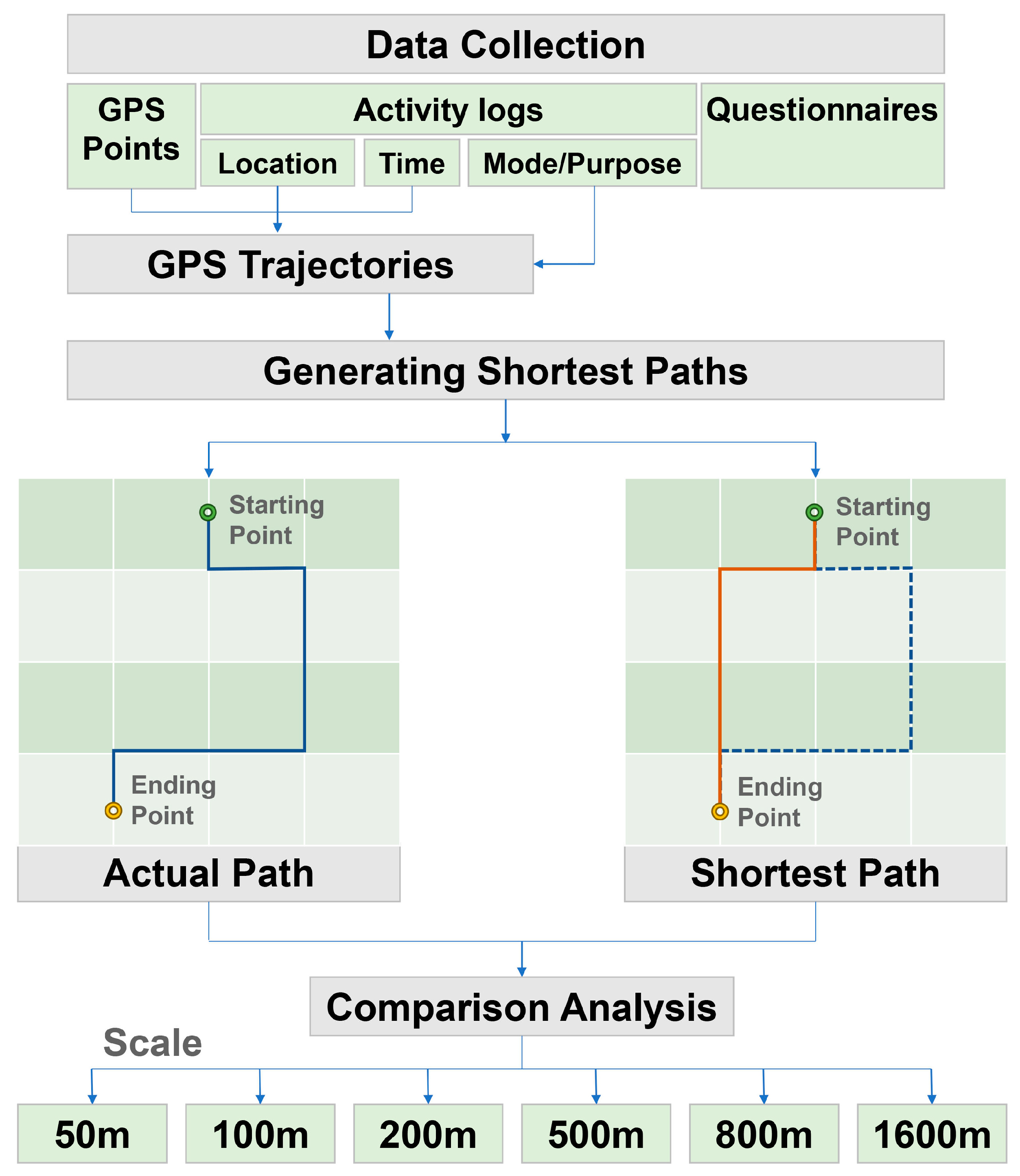
The methodology of this study is shown in Figure 1. GPS point data were collected and GPS travel trajectories were generated based on participants’ self-reported activity logs and questionnaires. The leisure walking trajectories were screened out, and paired shortest paths were generated based on Dijkstra’s algorithm. A grid-based buffer approach was used, and the built environment characteristics were calculated. Paired T-tests were conducted at different scales to compare built environment characteristics between the empirical route and the shortest calculated routes.
2.1. GPS Data Collection
Data were collected on the tracks of adults in Nanjing, China, from April to June 2019. In order to evenly divide the age groups, all participants were 20 years old or older. With the help of a local survey company, 300 adult volunteers were recruited from seven of the 11 districts in the city, excluding the four suburban districts. Participants were equally distributed by gender and proportionally by the population of each district. Participants were outfitted with portable GPS loggers (Brand: TuQiang; Model: GT 310) and instructed to wear them for one week to comprehensively record their travel behavior [42]. Each logger had a SIM card allowing for real-time location data recording via satellite, base station, or WiFi signal. Locations were recorded for participants every 30 s. The back-end system automatically generated records of GPS location points online. Using ArcGIS 10.5, all participants’ travel trajectories were plotted and manually matched to roads.
While wearing the GPS loggers, participants completed activity logs and questionnaires. Activity logs recorded the departure location and destination, departure and arrival time, transportation mode, and travel purpose for each trip the participants made during the seven days. The questionnaire included the respondents’ personal social and economic attributes, personal preferences, self-rated health status, and perceptions of the built environments they experience. Pedestrian route choice attributes were collected directly through travel logs, avoiding the issues that often plague route logging research [43].
2.2. GPS Data Processing
All recorded GPS points were connected manually in chronological order to generate tracks using ArcGIS 10.5. Based on the time, starting location, and ending location recorded in the participant’s self-reported activity logs, the GPS points recorded at the corresponding time were manually connected into tracks in ArcGIS 10.5. This is a simple but effective method that avoids the occasional errors in GPS positioning. Each trace showed the start time, end time, and purpose of the trip. A total of 7544 traces were retained out of 11,309 assessed for matching activity logs and questionnaires. Tracks that were made while cycling or using public transportation were excluded, leaving 2304 tracks determined to be via walking. Most walking trips were utilitarian. Using activity logs, data were limited to leisure walking trips, including dog walking, exercise (walking to a fitness facility was not included), and walking (for no purpose), and this dataset included 501 trips. Circumstances where the departure and return trajectories overlap were merged into a single trip. Loop paths were separated into two trajectories at the farthest point from the starting point. Finally, after filtering repeated traces and routes with no more than one turn, a total of 268 tracks were obtained from 105 participants.
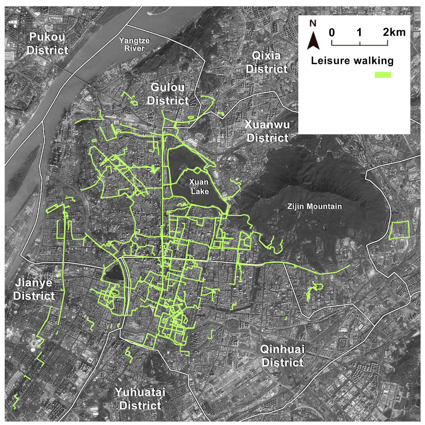
The set of GPS traces of leisure walking retained for this study is presented in Figure 2. The sample was found to be more concentrated in and around downtown, with a decrease in pedestrian activity towards the outskirts.
2.3. The Grid-Based Buffer Method
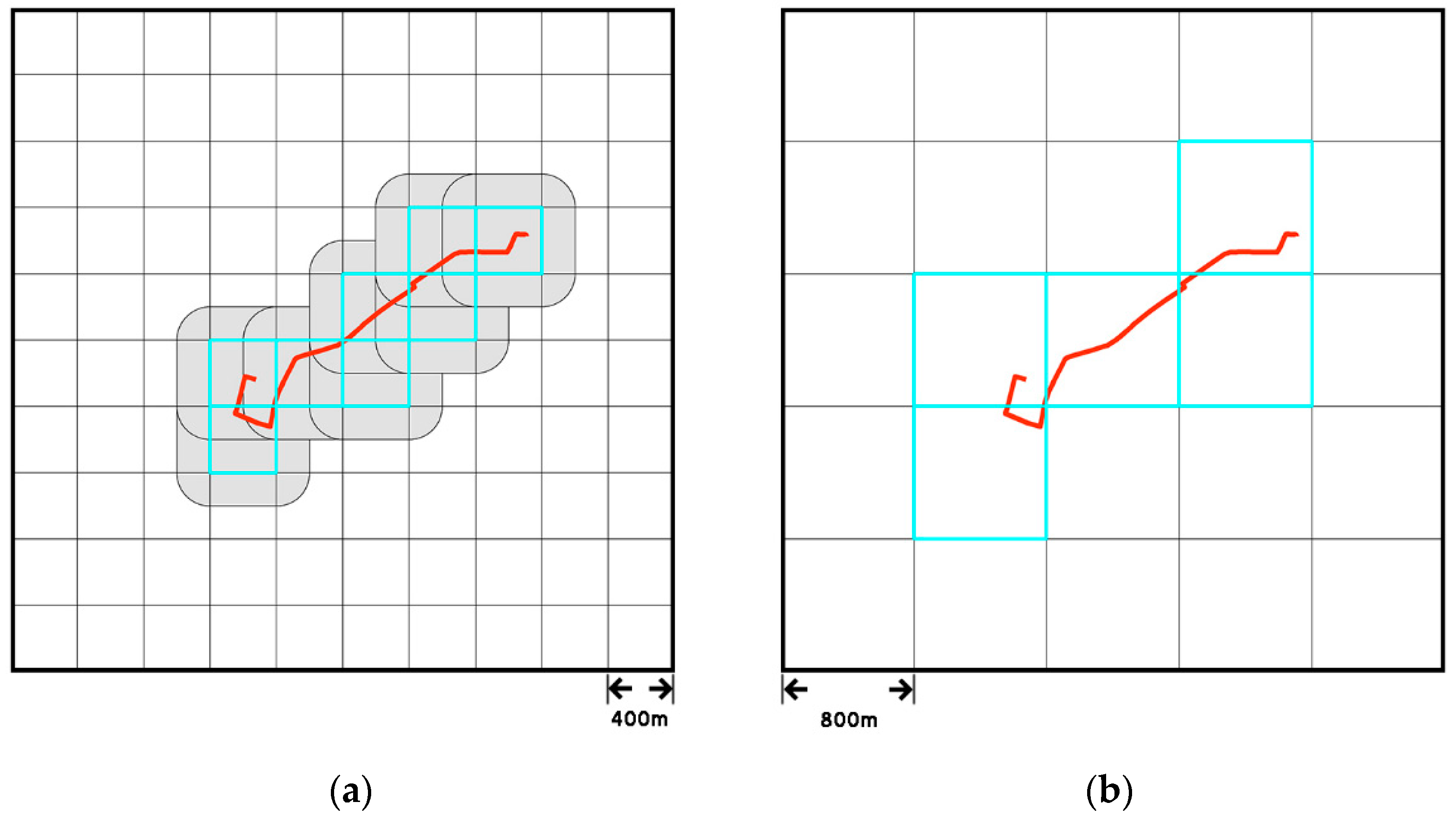
The association between the built environment and active transport varies depending on how the built environment context is defined [23,44]. It is typical to construct a line-based buffer around fine-scale routes collected using GPS technology. By matching routes to a real road network, a better representation of the local environment as it is experienced and perceived by participants may be captured for analysis [22,31,32]. However, the method assumes that the spatial context of the buffer area along a path is homogeneous, and calculates the average value within the entire buffer range. This would only rarely be an accurate representation of the built environment experienced by pedestrians. A grid-based method is one way to circumvent this limitation [28]. The classic grid-based method was improved by constructing a radial buffer based on original grid cells (Figure 2). A fishnet-based buffer was conducted to effectively represent heterogeneity in built environment characteristics. Buffer construction entailed two steps using different-sized grid cells constructed around routes. First, 400 m grids were constructed around routes, and then were extended by 200 m to form the 800 m buffers. Using the improved grid-based method, 8 grid cells (Figure 3a) were obtained versus only 5 grid cells (Figure 3b) using the classic method. Thus, this improved grid-based buffer approach allows a larger number of samples of built environment characteristics along routes.
Buffer sizes are normally set to capture aspects of the built environment involved in the health-related behavior of the residents, depending on the health issue being explored, the assumed mechanisms that impact health, and specific health outcomes [27,29,31,45,46]. The scale most frequently used for built environment examinations is 200 m to 250 m [29,46,47], which is equivalent to a 2.5 min walking distance for adults on average. The 800 m and 1600 m buffer sizes, equivalent to 10 min and 20 min of walking time, are also often used in relevant studies [22,43]. Other spatial scales that have been used include 300 m, 400 m [45], 500 m [48], and 1 km [31]. A qualitative study in the UK demonstrated that 1.6 km fully characterizes the boundaries of the walking neighborhood as perceived by pedestrians [21]. Therefore, the maximum buffer scale in this study was set to 1.6 km. Considering that many studies found that walking is associated with the built environment at relatively small scales [28,49] and that leisure walking distances tend to be short, the buffer sizes of 50 m, 100 m, 200 m, 500 m, 800 m, and 1600 m were used for analyses.
2.4. Selection of Built Environment Exposure Variables
Examinations of associations between walking and the built environment measure various characteristics. Based on built environment characteristics proposed by Cervero and Kockelman to capture three dimensions of variation that include density, diversity, and design [50], a total of 17 variables were selected (Table 1). These include the sum total of variables observed in a literature review of built environment impacts on walking route choice.
Fine-scale land-use data in the city of Nanjing were mapped based on a recent topographic map. Road network and points of interest (POIs) were obtained from the website of the Baidu Map Open Platform (https://lbsyun.baidu.com/, accessed on 3 January 2019). Data on the road network included attributes such as the name and type of each road, and the POI data included attributes such as name, address, and GPS coordinates.
Digital elevation model (DEM) data were obtained from ASTER GDEM 30M Digital Elevation Data. Waterbody data were obtained from the Landsat Waterbody Product of Inland China. NDVI data were obtained from MODIS NDVI, using a 16-day composite product of MYD13Q1 250M vegetation index. DEM data, waterbody data, and NDVI data were provided by the Geospatial Data Cloud site, Computer Network Information Center, Chinese Academy of Sciences (http://www.gscloud.cn, accessed on 7 October 2022).
2.5. Statistical Methods
Comparing actual routes with the shortest possible route is an effective method for studying the factors that influence the residents’ route choice, and is commonly used in similar research [28,46,48,52,53].
Characteristics of actual routes to those of shortest possible paths were compared to evaluate the sign and significance of built environment characteristics. The shortest paths were generated using the standard Dijkstra Algorithm based on the actual leisure walking routes. For this, the starting and ending points of real routes were extracted, a road network model was created based on the urban road network, and corollary shortest paths were generated using Network Analyst tools in ArcGIS 10.5.
For both actual and shortest paths, the mean (MEAN), standard deviation (SD), 1st quartile, median, 3rd quartile, minimum (MIN), and maximum (MAX) of the built environment characteristics were calculated in all intersecting grid cells.
Paired T-tests were conducted using SPSS 20 to compare built environment characteristics between the empirical route and the shortest calculated routes.
3. Results
3.1. Descriptive Analysis
Among the 105 participants represented in the final dataset, there was a male-to-female ratio of nearly 4:5 with 46 men and 59 women having relevant leisure walking traces. The ages of the participants ranged from 21 to >61 years. For analyses, participants were divided by sex and age (Table 2).
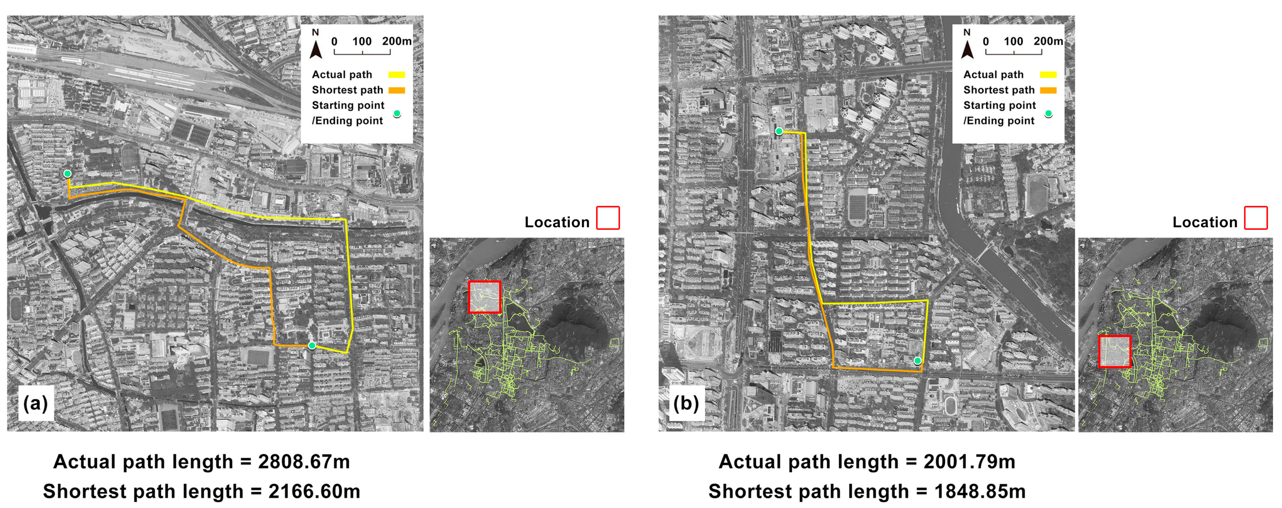
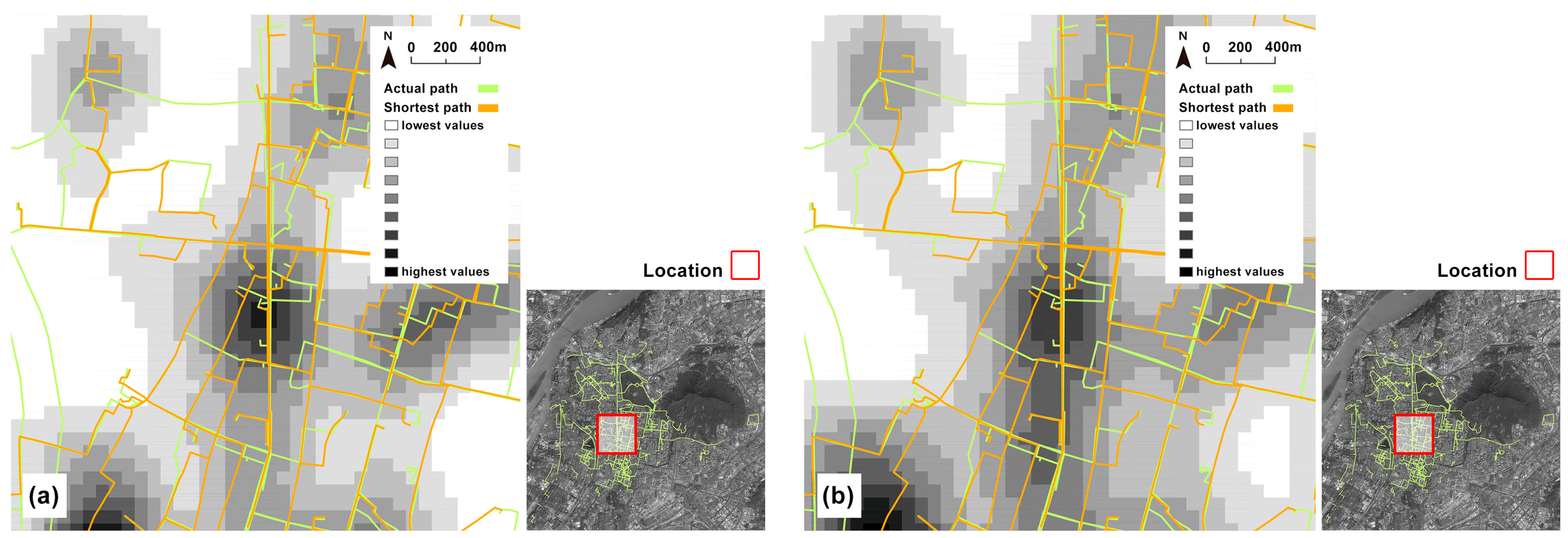
The average lengths of the 268 empirical walking paths were compared with the shortest paths based on real origin and destination points. As is shown in Figure 4, although the shortest paths partially overlapped with the actual paths, the actual path was significantly longer than the shortest paths. In Figure 4a, the actual path was 642.07 m longer than the shortest path, and in Figure 4b, the actual path was 152.94 m longer than the shortest path.
The actual walking path length was 1707 m on average, and the actual paths were an average of 24.97% longer (Table 3). The standard deviation of the shortest paths was also significantly smaller than the actual paths, indicating that the dispersion of the shortest path’s length was relatively small.
3.2. Statistical Analysis
Differences in built environment variables between empirical and shortest walking routes are presented in Table 4. At the 1600 m scale, there are two paths where the actual path and the shortest path intersect with the same grids, thus generating the same buffer zone. These two paths were removed from the paired T-test at the 1600 m scale. The most preferred characteristics for leisure walkers were building coverage and FAR, and the most avoided characteristic was intersection density, which showed significant associations at most scales from 50 m to 1600 m. Numerous built environment variables were not at all or only weakly associated with leisure walking. The industrial area was the only variable without a significant test at any scale. Furthermore, the slope was found to be associated with leisure walking only at the 800 m scale, and the green area was found to be associated with leisure walking at only 50 m and 500 m scales.
For most of the built environment variables, the direction of the mean difference was consistently negative (Table 4). Intersection density and slope were exceptions with positive mean differences. A few variables were inconsistent in the direction of impacts between scales. For example, the mean difference of recreational facilities was negative at the 1600 m scale and positive at scales ranging from 50 m to 200 m.
The most significant correlations were found at the 100 m scale, though relatively strong correlations were found at the 50 m and 200 m scales. Overall, the correlations between leisure walking and built environment variables were stronger at smaller scales and weaker at larger scales. However, more significant associations were found at the 1600 m scale than at the 800 m scale.
Different built environment variables influence leisure walking based on different spatial-behavioral interaction mechanisms, as reflected in different statistical variables testing significantly (see Appendix A). Of all the statistical variables, MEAN presented the highest number of significant results. More MAX comparisons were significant than MIN, including in land-use mix, slope, NDVI, and intersection density. Of the variables with significantly different MIN values, most were based on POI data, such as food outlets and healthcare facilities. Fewer comparisons of SDs were significant, which means the degree of fluctuation of the variables played an important role. These variables were density indicators and descriptions of land use area, including residential, green, commercial, and administrative areas.
4. Discussion
4.1. The Association between Density and Leisure Walking Route Choice
4.1.1. Residential Density
Our results showed that residential density was associated with leisure walking at scales ranging from 50 m to 200 m, which is consistent with findings from active transportation studies [54,55]. It has been previously suggested that excessive residential density may have a negative impact on walking choices [56], but this was not found in our study. In addition, the diversity of residential density as reflected by SD was found to be significant, suggesting that pedestrians favor heterogeneity in urban spatial patterns [57].
4.1.2. Building Coverage and Floor-to-Area Ratio
Housing and employment density have received extensive research attention, and urban spatial density is often neglected. As interrelated variables, building coverage and FAR showed similar patterns of correlation with leisure walking (Figure 5). The association between the means of these two variables and leisure walking diminished as the scale increased, though the significance between SDs remained constant. Participants seemed to prefer routes with higher building coverage and FAR at smaller scales, and more diverse spatial patterns at all scales. These results also support a pedestrian preference for spatial heterogeneity in urban environments.
4.1.3. Destination Density
According to our results, recreational and cultural facilities with leisure attributes were less impactful than utilitarian facilities such as healthcare, food, retail stores, and other public facilities. Consistent with these results, previous analyses found that utilitarian destinations showed stronger associations with walking than recreational POI [38]. Utilitarian destinations emerge consistently as important indicators of walkable environments [58,59]. Surprisingly, pedestrians chose to avoid recreational facilities during leisure walking [60], suggesting that indoor recreational activities such as massage, sauna, and karaoke are not favorable for leisure walking.
Similar patterns of association with leisure walking were found between food outlets and healthcare facilities, with participants avoiding both at the 200 m scale. Hospitals, nursing homes, and other healthcare facilities may be associated with illness, which could explain participants’ avoidance during leisure walking. Meanwhile, areas with a high density of food stores are often characterized by high traffic flow and overly crowded environments, which may explain their avoidance by leisure walkers.
Compared to food outlets, the retail facilities category was associated with leisure walking at larger scales from 500 m to 1600 m. Similarly, commercial area was significantly associated with leisure walking at the 50 m and 100 m scales, with participants showing a preference. This suggests that it is not the retail facilities themselves that attracted participants, but rather the adequate density and diversity in destinations that may accompany them (Figure 6).
Among other structure use types, participants did not show significant preferences. Pedestrians preferred heterogeneity in facility types and functional services along the route, but also preferred both at a greater distance from those offering indoor services. Homogenous areas were generally avoided.
4.2. The Association between Diversity and Leisure Walking Route Choice
Fernandes et al. found that land-use mix was associated with leisure walking at 500 m and 1000 m [61]; the 1600 m scale was found to be more significant in this article. The reason for the difference may be due to the larger block sizes in Nanjing versus Porto Alegre, Brazil, the study area of Fernandes et al. At smaller scales, the association between land-use mix and leisure walking was significantly weaker. Beyond the impact of block size, it is also possible that larger scales may more accurately capture measures of land-use mix.
At scales ranging from 50 m to 200 m, land-use mix was associated with leisure walking when comparing the MAX and SD terms. As is shown in Figure 7, geographic scale may influence the measurement of land-use mix [24]. This may provide a further indication of a preference for increased heterogeneity in land use at smaller scales. Overall, leisure walkers may prefer environments with a higher land-use mix while avoiding less built environments at all scales.
4.3. The Association between Design and Leisure Walking Route Choice
4.3.1. Intersection Density
According to our results, walkers avoided a built environment with high intersection density at all scales except 800 m. The negative effect of intersection density on leisure walking is a common finding [54,62]. However, this conflicts with the fact that many studies use intersection density as a dimension for measuring walkability [11]. Moran et al. noted the paradox that connectivity may be positively associated with walking at the level of an area, but at the individual level, connectivity may negatively impact walking route choice [63]. The correlation between intersection density and leisure walking was found to diminish from 500 m to 800 m but to increase at 1600 m. The measurement of intersection density may also be affected by neighborhood size [64], and that is likely the case here given that our largest buffer size of 1600 m was close to the block size.
4.3.2. Slope
Slope was found to be significant only at the 800 m scale, with participants primarily avoiding larger slopes during leisure walking. This is contrary to the findings of some studies that residents seek higher slopes in leisure walking for views and greater exertion in the course of exercise [38,65]. In addition, a significant difference in SD indicates that leisure walkers preferred a built environment with less variation in slope. This may be related to the urban layout of Nanjing, where the slope is small in places suitable for walking and higher slopes are mainly located in places that are difficult to reach on foot or in residential areas.
4.3.3. Water Area
Water was previously found to be associated with attracting leisure walking [33]. However, water area was found to be weakly associated with leisure walking, and only in terms of its MAX value. The MEAN value of the water area was not significantly associated with leisure walking at any scale. In our study area, there may be too few water bodies in the area where leisure walking mainly occurs. Larger water bodies may be more attractive to leisure walkers [40], which was proven in this article.
4.3.4. NDVI and Green Areas
Green space is often highly associated with walkability in built environments [11,66]; however, a strong association was not found in our results. Rather, our findings indicated that NDVI and green areas were weakly associated with leisure walking at multiple scales. This may be related to our method of measuring green space, which was based on remote sensing images and land-use data that may not have the resolution to reflect the true presence of living landscapes. In addition, cultural facilities also contained green landscapes such as parks and small historical gardens. If cultural facilities are included when examining the association between green space and leisure walking, the associations may increase in importance.
At the smaller scale of 50 m, leisure walkers may prefer more greenery. At scales greater than 500 m, leisure walkers may instead avoid environments with a lot of greenery because such spaces often mean that the surrounding area will provide fewer desirable functions to elicit trips.
5. Conclusions
Based on an improved grid-based buffer approach, by comparing the empirical paths and shortest path options, the impacts of built environment variables on leisure walking choices were examined across multiple scales of influence. Our study identified the most relevant spatial scales between leisure walking and the built environment, and discovered mechanisms by which the association between leisure walking and the built environment varies with scale.
The clearest associations between built environment variables and leisure walking were found at the 100 m scale, and there was an overall trend of increased instances of significant associations as scales decreased in size. Built environment variables affecting leisure walking route choice varied across scales, possibly corresponding to benefit pathways. Pedestrians seek more emotional benefits in their decision making for leisure walking than for utilitarian walking. As a result, pedestrians perceive the walking environment at a larger scale in leisure walking, and the most relevant spatial scale was larger than that of utilitarian walking. In addition, pedestrians’ perceptions of the walking environment decreased with distance, and thus the association between leisure walking and the built environment diminished with scale.
Built environment variables in all three dimensions, including density, diversity, and design, significantly impacted leisure walking choices. The strengths of associations of these variables varied. The built environment variables with functional attributes were found to have a more significant impact on leisure walking, with the strongest being intersection density, building coverage, and FAR. In addition, built environment variables with aesthetic attributes were found to promote leisure walking. Participants showed a preference for moderately compact urban forms, diverse options for destinations, and greener landscapes in leisure walking route choice.
Some of the associations between leisure walking and the built environment in this study differ from the findings of previous research. Influenced by the study case, the way leisure walking is defined, and the methodology used in this study, some findings in this study may have some limitations. Land-use mix was found to be more relevant to leisure walking at larger scales in this study. In addition, participants in leisure walks were found to avoid a built environment with high slopes and high variation in slope. Both of these two findings may be specific to the case study. This study did not find a clear link between green spaces and leisure walking, which may be due to the methodology approach used in this study.
In our study, the possible impact of population on the built environment preferences of leisure walkers was not considered. Studies have found that heterogeneity in population plays an important role in the association between walking and the built environment [67,68], and future attempts should be made to explore the effect of individual heterogeneity on route choice by considering more individual characteristics. In addition, the scale of grid-based buffers may influence measurements of the built environment [28]. This was verified at the 800 m scale, where the significance of several variables, such as land-use mix and intersection density, decreased compared to other scales. More methods of buffer construction should be explored in the future and the effectiveness and stability of these methods should be compared [31,32].
Author Contributions
Yifu Ge: Data curation, Software, Writing—Original draft preparation; Zhongyu He: Methodology, Writing—Reviewing and editing; Kai Shang: Analysis, Manuscript preparation. All authors have read and agreed to the published version of the manuscript.
Funding
This project received funding from the National Natural Science Foundation of China, grant number 51678288.
Data Availability Statement
Some data used during the study are confidential and may only be provided with restrictions.
Conflicts of Interest
The authors declare no conflict of interest.
Appendix A

Table A1.
Differences in built environment distribution along actual vs. shortest routes—SD, Median, Quartile 1, Quartile 3, MAX, MIN.
Table A1.
Differences in built environment distribution along actual vs. shortest routes—SD, Median, Quartile 1, Quartile 3, MAX, MIN.
| SD | 50 m | 100 m | 200 m | 500 m | 800 m | 1600 m | ||||||
| Mean Diff | p-Value | Mean Diff | p-Value | Mean Diff | p-Value | Mean Diff | p-Value | Mean Diff | p-Value | Mean Diff | p-Value | |
| Residential Density | −55.1188 | 0.0000 ** | −111.6731 | 0.0071 ** | −303.3417 | 0.0097 ** | −885.3762 | 0.1016 | −525.7040 | 0.6104 | 1574.7708 | 0.5461 |
| Building Coverage | −0.0230 | 0.0000 ** | −0.0097 | 0.0000 ** | −0.0034 | 0.0193 * | −0.0020 | 0.0394 * | −0.0019 | 0.0141 * | −0.0002 | 0.7031 |
| FAR | −0.2405 | 0.0000 ** | −0.1342 | 0.0000 ** | −0.0422 | 0.0016 ** | −0.0188 | 0.0140 * | −0.0055 | 0.3668 | −0.0028 | 0.4777 |
| Food Outlets | −0.0561 | 0.2226 | −0.0022 | 0.9751 | 4.5174 | 0.0000 ** | −0.1896 | 0.5082 | −0.6937 | 0.1581 | −0.9176 | 0.5139 |
| Healthcare Facilities | 0.0026 | 0.7630 | −0.0252 | 0.2607 | −0.0871 | 0.1102 | −0.3624 | 0.0005 ** | −0.2798 | 0.0633 | −0.8692 | 0.0153 |
| Recreational Facilities | 0.0106 | 0.6504 | 0.0465 | 0.3017 | 0.0964 | 0.2690 | −0.0855 | 0.5611 | −0.0376 | 0.8771 | −0.1289 | 0.8418 |
| Cultural Facilities | 0.0771 | 0.0000 ** | −0.0118 | 0.5870 | −0.0439 | 0.3739 | −0.1906 | 0.0451 * | −0.2966 | 0.1348 | −0.4109 | 0.2244 |
| Retail Facilities | −0.2001 | 0.0521 | −0.1124 | 0.6590 | −0.5687 | 0.1979 | −2.0858 | 0.0126 * | −2.2239 | 0.0553 | −3.2938 | 0.2555 |
| Industrial Area | −9.7429 | 0.2026 | −15.1867 | 0.5414 | −40.4863 | 0.5612 | 187.1937 | 0.6098 | 671.0774 | 0.2683 | 220.5837 | 0.9040 |
| Commercial Area | −41.4496 | 0.0000 ** | −77.1425 | 0.0012 ** | −63.5449 | 0.3672 | −186.8354 | 0.4528 | −35.2280 | 0.9412 | 1413.9198 | 0.2078 |
| Administrative Area | −26.9332 | 0.0037 ** | −69.9108 | 0.0183 * | −173.9744 | 0.0772 | −989.2110 | 0.0344 * | −1797.0930 | 0.0562 | −394.4470 | 0.8353 |
| Intersection Density | 0.0001 | 0.0000 ** | 0.0000 | 0.0000 ** | 0.0000 | 0.0503 * | 0.0000 | 0.6879 | 0.0000 | 0.3814 | 0.0000 | 0.9455 |
| Slope | −0.0032 | 0.9687 | 0.0057 | 0.9435 | 0.0804 | 0.2845 | −0.1346 | 0.0683 | 0.1264 | 0.0460 * | 0.0073 | 0.8958 |
| NDVI | −42.1072 | 0.1400 | −544.4111 | 0.0000 ** | 1051.4029 | 0.0000 ** | 122.0965 | 0.0820 | 97.6043 | 0.1566 | 33.0108 | 0.5359 |
| Water Area | −5.5421 | 0.1863 | −22.2492 | 0.1549 | −78.6871 | 0.1389 | −185.1266 | 0.5023 | −774.4159 | 0.2686 | −1546.2043 | 0.5148 |
| Green Area | −23.1767 | 0.0128 * | −33.5000 | 0.2348 | −12.1973 | 0.8763 | −141.8990 | 0.6763 | −736.8204 | 0.3529 | 745.4136 | 0.7508 |
| Land-Use Mix | −0.0072 | 0.0011 ** | −0.0057 | 0.0024 * | −0.0038 | 0.0394 * | −0.0015 | 0.4196 | −0.0021 | 0.1786 | 0.0027 | 0.0778 |
| Median | 50 m | 100 m | 200 m | 500 m | 800 m | 1600 m | ||||||
| Mean diff | p-value | Mean diff | p-value | Mean diff | p-value | Mean diff | p-value | Mean diff | p-value | Mean diff | p-value | |
| Residential Density | −59.1987 | 0.0138 * | −198.5580 | 0.0166 * | −601.4210 | 0.0208 * | −778.0657 | 0.4707 | −1421.5208 | 0.3229 | −5701.8094 | 0.0588 |
| Building Coverage | −0.0295 | 0.0000 ** | −0.0157 | 0.0004 ** | −0.0086 | 0.0076 ** | −0.0042 | 0.0715 | −0.0019 | 0.2644 | −0.0019 | 0.1310 |
| FAR | −0.1117 | 0.0002 ** | −0.0645 | 0.0200 * | −0.0387 | 0.1174 | −0.0307 | 0.0722 | −0.0149 | 0.2648 | −0.0166 | 0.0657 |
| Food Outlets | 0.0093 | 0.2980 | 0.0560 | 0.0843 | 4.1306 | 0.0000 ** | 0.1343 | 0.8384 | −0.8097 | 0.5225 | −4.0226 | 0.2267 |
| Healthcare Facilities | 0.0019 | 0.3182 | 0.0224 | 0.0453 * | 0.0840 | 0.0145 * | 0.2985 | 0.1067 | −0.1063 | 0.4997 | −0.1823 | 0.7417 |
| Recreational Facilities | 0.0093 | 0.0956 | 0.0224 | 0.4358 | 0.1063 | 0.1968 | −0.2593 | 0.3843 | −0.4496 | 0.4306 | −2.9774 | 0.0462 * |
| Cultural Facilities | 0.0037 | 0.3182 | −0.0149 | 0.2490 | −0.0299 | 0.3046 | −0.1175 | 0.5145 | −0.3899 | 0.0459 * | 0.4530 | 0.4007 |
| Retail Facilities | −0.0429 | 0.1533 | 0.0000 | 1.0000 | −0.0541 | 0.8663 | −0.7034 | 0.7006 | −4.0056 | 0.1229 | −8.7105 | 0.1726 |
| Industrial Area | 1.7134 | 0.7860 | 0.0335 | 0.9989 | −21.5925 | 0.8001 | −479.3247 | 0.3321 | 260.5927 | 0.6004 | −1084.0562 | 0.5333 |
| Commercial Area | −49.0601 | 0.0013 * | −86.1962 | 0.0333 * | −99.2591 | 0.4518 | −846.7352 | 0.0931 | −2368.3364 | 0.0079 ** | −5315.8372 | 0.0117 * |
| Administrative Area | −3.1292 | 0.7148 | 16.3814 | 0.5629 | 182.6051 | 0.1155 | 784.3972 | 0.0933 | 2213.9516 | 0.0552 | −1577.8573 | 0.4795 |
| Intersection Density | 0.0000 | 0.0000 ** | 0.0000 | 0.0000 ** | 0.0000 | 0.0000 ** | 0.0000 | 0.0131 * | 0.0000 | 0.8361 | 0.0000 | 0.0039 ** |
| Slope | 0.0626 | 0.5681 | 0.1467 | 0.2498 | 0.1952 | 0.1114 | 0.0061 | 0.9649 | 0.1015 | 0.3566 | 0.0176 | 0.7869 |
| NDVI | / | / | 1.7207 | 0.0000 ** | −115.5778 | 0.0688 | 229.0956 | 0.0952 | 121.5952 | 0.3615 | 37.9620 | 0.6058 |
| Water Area | 1.1472 | 0.3745 | 11.1792 | 0.2859 | 47.5011 | 0.4358 | 37.6946 | 0.9260 | −150.6220 | 0.8562 | −2528.6699 | 0.2819 |
| Green Area | 2.7456 | 0.8562 | 31.5662 | 0.5272 | 141.1113 | 0.3269 | 824.8978 | 0.1110 | 66.4150 | 0.9405 | 4447.3963 | 0.1440 |
| Land-Use Mix | −0.0051 | 0.2856 | 0.0033 | 0.4522 | 0.0046 | 0.2549 | −0.0028 | 0.4284 | −0.0019 | 0.4569 | −0.0045 | 0.0093 ** |
| Quartile1 | 50 m | 100 m | 200 m | 500 m | 800 m | 1600 m | ||||||
| Mean diff | p-value | Mean diff | p-value | Mean diff | p-value | Mean diff | p-value | Mean diff | p-value | Mean diff | p-value | |
| Residential Density | −21.9707 | 0.2970 | −86.5448 | 0.2362 | −479.1059 | 0.0403 * | −91.7899 | 0.9285 | −2547.0967 | 0.0978 | −6079.9820 | 0.1024 |
| Building Coverage | −0.0152 | 0.0003 ** | −0.0111 | 0.0075 ** | −0.0052 | 0.1355 | 0.0002 | 0.9281 | 0.0000 | 0.9856 | −0.0007 | 0.6088 |
| FAR | −0.0491 | 0.0087 ** | −0.0466 | 0.0363 * | −0.0334 | 0.1414 | −0.0176 | 0.2476 | −0.0088 | 0.4902 | −0.0110 | 0.2376 |
| Food Outlets | −0.0028 | 0.4679 | 0.0625 | 0.0160 * | 2.5485 | 0.0000 ** | −0.3993 | 0.5001 | −1.2481 | 0.2495 | −2.6222 | 0.3989 |
| Healthcare Facilities | / | / | 0.0093 | 0.0771 | 0.0690 | 0.0228 * | 0.1483 | 0.3487 | −0.0345 | 0.8042 | 0.4192 | 0.4181 |
| Recreational Facilities | 0.0037 | 0.3182 | 0.0401 | 0.0052 ** | 0.1427 | 0.0174 * | 0.0289 | 0.9223 | −0.5961 | 0.2356 | −2.1767 | 0.1346 |
| Cultural Facilities | 0.0037 | 0.3182 | 0.0037 | 0.3182 | −0.0177 | 0.2018 | 0.0634 | 0.6569 | −0.0056 | 0.9759 | 0.5761 | 0.3561 |
| Retail Facilities | −0.0112 | 0.4489 | 0.0672 | 0.2951 | 0.1828 | 0.3732 | 0.4524 | 0.6984 | −3.2164 | 0.1632 | −6.3148 | 0.3192 |
| Industrial Area | −3.1066 | 0.2064 | −8.0205 | 0.4718 | −45.4256 | 0.3101 | −837.3911 | 0.0589 | −694.1207 | 0.1792 | −573.1235 | 0.7707 |
| Commercial Area | −21.6580 | 0.0095 ** | −32.8740 | 0.1897 | −39.0885 | 0.7304 | −452.0332 | 0.3769 | −1276.8381 | 0.1363 | −4544.6456 | 0.0338 |
| Administrative Area | 0.4341 | 0.9411 | 19.4088 | 0.3283 | 94.9620 | 0.3144 | 1038.2414 | 0.0205 * | 2449.3601 | 0.0141 * | −2784.1654 | 0.2619 |
| Intersection Density | 0.0000 | 0.0139 * | 0.0000 | 0.0000 ** | 0.0000 | 0.0000 ** | 0.0000 | 0.0053 ** | 0.0000 | 0.7116 | 0.0000 | 0.0092 ** |
| Slope | 0.0275 | 0.6565 | 0.1108 | 0.2270 | 0.0930 | 0.3715 | −0.0225 | 0.8399 | 0.0600 | 0.5355 | 0.0415 | 0.5757 |
| NDVI | / | / | 0.9457 | 0.0000 ** | −103.1807 | 0.0760 | 199.9157 | 0.0744 | 85.6543 | 0.4685 | 47.2391 | 0.5135 |
| Water Area | / | / | 5.1294 | 0.0926 | 38.7126 | 0.2116 | 60.5615 | 0.7396 | −74.5535 | 0.8734 | −1048.1534 | 0.4358 |
| Green Area | 3.8010 | 0.5030 | 26.5096 | 0.3024 | 108.4552 | 0.2309 | 963.7670 | 0.0227 * | 1496.9435 | 0.0670 | 2856.2625 | 0.3083 |
| Land-Use Mix | −0.0033 | 0.4417 | 0.0034 | 0.4290 | 0.0063 | 0.1096 | 0.0004 | 0.9035 | 0.0006 | 0.8480 | −0.0063 | 0.0113 * |
| Quartile3 | 50 m | 100 m | 200 m | 500 m | 800 m | 1600 m | ||||||
| Mean diff | p-value | Mean diff | p-value | Mean diff | p-value | Mean diff | p-value | Mean diff | p-value | Mean diff | p-value | |
| Residential Density | −108.2561 | 0.0001 ** | −258.9185 | 0.0041 ** | −813.4984 | 0.0047 ** | −1061.2719 | 0.3599 | −2076.2318 | 0.2074 | −5923.0591 | 0.0512 |
| Building Coverage | −0.0399 | 0.0000 ** | −0.0183 | 0.0002 ** | −0.0085 | 0.0159 * | −0.0044 | 0.0398 * | −0.0030 | 0.0508 | −0.0014 | 0.2354 |
| FAR | −0.2130 | 0.0000 ** | −0.1488 | 0.0001 ** | −0.0697 | 0.0329 * | −0.0339 | 0.0540 | −0.0148 | 0.3111 | −0.0051 | 0.5971 |
| Food Outlets | 0.0243 | 0.4532 | 0.0802 | 0.4081 | 6.4310 | 0.0000 ** | −0.3125 | 0.6636 | −1.5924 | 0.2407 | −1.5197 | 0.6746 |
| Healthcare Facilities | 0.0028 | 0.6556 | 0.0084 | 0.6579 | 0.1558 | 0.0354 * | −0.0075 | 0.9657 | −0.0252 | 0.9155 | −0.2321 | 0.7056 |
| Recreational Facilities | 0.0504 | 0.0047 ** | 0.0774 | 0.1350 | 0.2099 | 0.0839 | −0.2444 | 0.4928 | −0.5494 | 0.3889 | −1.5113 | 0.3546 |
| Cultural Facilities | 0.0093 | 0.0956 | −0.0261 | 0.2120 | −0.0746 | 0.3195 | −0.3918 | 0.0981 | −0.4142 | 0.1772 | −0.2152 | 0.6866 |
| Retail Facilities | −0.0513 | 0.3983 | −0.2332 | 0.3145 | −1.0000 | 0.0739 | −3.2080 | 0.0962 | −8.1269 | 0.0058 ** | −9.6504 | 0.1393 |
| Industrial Area | −14.8887 | 0.2117 | −35.4831 | 0.3466 | −29.8539 | 0.7949 | −171.8174 | 0.8003 | 1626.9612 | 0.0555 | −1896.0122 | 0.4061 |
| Commercial Area | −69.6132 | 0.0002 ** | −94.5841 | 0.0941 | −149.7847 | 0.3696 | −789.5937 | 0.1186 | −1790.0097 | 0.0615 | −1611.7209 | 0.4035 |
| Administrative Area | −20.8875 | 0.2139 | −18.2748 | 0.7537 | 4.3329 | 0.9815 | −131.9797 | 0.8557 | 266.4269 | 0.8592 | −2246.3840 | 0.3272 |
| Intersection Density | 0.0001 | 0.0000 ** | 0.0000 | 0.0000 ** | 0.0000 | 0.0000 ** | 0.0000 | 0.5514 | 0.0000 | 0.9249 | 0.0000 | 0.0312 * |
| Slope | 0.0227 | 0.8918 | 0.2096 | 0.2132 | 0.2898 | 0.0650 | −0.0561 | 0.7400 | 0.2146 | 0.1009 | 0.0621 | 0.5657 |
| NDVI | / | / | −1.5096 | 0.7369 | 437.3705 | 0.0001 ** | 335.6175 | 0.0280 * | 247.1930 | 0.0975 | 115.2982 | 0.3612 |
| Water Area | 7.7966 | 0.2905 | 24.6656 | 0.3551 | 38.9723 | 0.7037 | −677.0517 | 0.1747 | −284.7681 | 0.8378 | −516.1703 | 0.9026 |
| Green Area | −7.9489 | 0.7358 | 6.3919 | 0.9287 | −137.2260 | 0.4897 | 171.5473 | 0.7823 | −776.1916 | 0.5314 | 5433.8606 | 0.1455 |
| Land-Use Mix | −0.0108 | 0.0558 | −0.0071 | 0.1443 | −0.0004 | 0.9220 | −0.0045 | 0.2056 | −0.0022 | 0.2316 | −0.0031 | 0.0219 * |
| MAX | 50 m | 100 m | 200 m | 500 m | 800 m | 1600 m | ||||||
| Mean diff | p-value | Mean diff | p-value | Mean diff | p-value | Mean diff | p-value | Mean diff | p-value | Mean diff | p-value | |
| Residential Density | −159.0742 | 0.0000 ** | −397.9019 | 0.0010 ** | −1013.8921 | 0.0010 ** | −1874.1173 | 0.1412 | −2352.5311 | 0.2627 | −3117.2816 | 0.4109 |
| Building Coverage | −0.1115 | 0.0000 ** | −0.0499 | 0.0000 ** | −0.0194 | 0.0000 ** | −0.0054 | 0.0087 ** | −0.0038 | 0.0072 ** | −0.0011 | 0.2365 |
| FAR | −1.2568 | 0.0000 ** | −0.7162 | 0.0000 ** | −0.2156 | 0.0000 ** | −0.0768 | 0.0026 ** | −0.0197 | 0.2376 | −0.0154 | 0.0687 |
| Food Outlets | −0.4403 | 0.1273 | −0.0299 | 0.9229 | 17.4590 | 0.0000 ** | −0.8806 | 0.3404 | −3.8657 | 0.0168 | −5.6654 | 0.0974 |
| Healthcare Facilities | −0.0299 | 0.5667 | −0.1642 | 0.1696 | −0.6157 | 0.0123 * | −1.4627 | 0.0011 ** | −1.2015 | 0.0086 ** | −1.7293 | 0.0039 ** |
| Recreational Facilities | −0.0224 | 0.8947 | 0.0299 | 0.8877 | 0.1679 | 0.6006 | −0.0970 | 0.8535 | −1.2090 | 0.1042 | −3.1203 | 0.0356 |
| Cultural Facilities | 0.4515 | 0.0000 ** | −0.1045 | 0.2600 | −0.3022 | 0.1077 | −0.6418 | 0.0485 * | −0.9627 | 0.1051 | −0.6842 | 0.3019 |
| Retail Facilities | −1.0970 | 0.1511 | −0.6642 | 0.5561 | −2.4851 | 0.1628 | −6.7052 | 0.0257 * | −7.4739 | 0.0417 * | −14.5451 | 0.0201 * |
| Industrial Area | −30.7211 | 0.2429 | −35.6760 | 0.6678 | −228.7214 | 0.2938 | −538.4549 | 0.5902 | 2129.8348 | 0.1767 | −2099.0982 | 0.5535 |
| Commercial Area | −174.9229 | 0.0000 ** | −342.4651 | 0.0001 ** | −294.8284 | 0.2177 | −1018.9650 | 0.1666 | −867.9059 | 0.5101 | −1908.3660 | 0.3430 |
| Administrative Area | −105.5171 | 0.0005 ** | −240.9912 | 0.0092 ** | −521.1862 | 0.0702 | −2300.7370 | 0.0712 | −2898.2937 | 0.1959 | −4534.0343 | 0.1666 |
| Intersection Density | 0.0002 | 0.0000 ** | 0.0001 | 0.0010 ** | 0.0000 | 0.0087 ** | 0.0000 | 0.2537 | 0.0000 | 0.7318 | 0.0000 | 0.0224 * |
| Slope | −0.1409 | 0.6414 | −0.0502 | 0.8587 | 0.3309 | 0.1563 | −0.2905 | 0.1887 | 0.3707 | 0.0290 * | 0.0837 | 0.5628 |
| NDVI | −267.1642 | 0.1530 | −2545.8123 | 0.0000 ** | 3026.6069 | 0.0000 ** | 407.3147 | 0.0202 * | 326.4592 | 0.0685 | 151.9385 | 0.3166 |
| Water Area | −43.2795 | 0.0129 ** | −142.1859 | 0.0191 * | −365.5755 | 0.0493 * | −801.9305 | 0.3284 | −2741.2646 | 0.1458 | −3610.8585 | 0.5200 |
| Green Area | −90.4092 | 0.0006 ** | −110.1344 | 0.1588 | 0.3437 | 0.9989 | −401.8442 | 0.7164 | −794.2174 | 0.7244 | 1458.6517 | 0.7710 |
| Land-Use Mix | −0.0248 | 0.0008 ** | −0.0182 | 0.0021 ** | −0.0069 | 0.1220 | −0.0077 | 0.0404 * | −0.0012 | 0.5633 | −0.0031 | 0.0801 |
| MIN | 50 m | 100 m | 200 m | 500 m | 800 m | 1600 m | ||||||
| Mean diff | p-value | Mean diff | p-value | Mean diff | p-value | Mean diff | p-value | Mean diff | p-value | Mean diff | p-value | |
| Residential Density | 19.3362 | 0.3476 | 24.5091 | 0.7395 | 44.8787 | 0.8342 | 1049.5813 | 0.3140 | −1182.8099 | 0.5896 | −4089.9809 | 0.4144 |
| Building Coverage | 0.0028 | 0.2545 | −0.0019 | 0.5451 | −0.0030 | 0.3267 | 0.0012 | 0.5952 | 0.0028 | 0.1564 | −0.0008 | 0.5958 |
| FAR | 0.0165 | 0.1080 | −0.0081 | 0.6157 | −0.0165 | 0.3762 | −0.0025 | 0.8661 | 0.0007 | 0.9579 | −0.0059 | 0.5451 |
| Food Outlets | / | / | 0.0299 | 0.0453 | 1.4813 | 0.0000 ** | −0.0112 | 0.9781 | −0.9179 | 0.2963 | −1.3120 | 0.6845 |
| Healthcare Facilities | / | / | 0.0037 | 0.3182 | 0.0560 | 0.0429 * | 0.2052 | 0.2002 | −0.0187 | 0.8962 | 0.6617 | 0.2663 |
| Recreational Facilities | 0.0037 | 0.3182 | 0.0187 | 0.0251 * | 0.0970 | 0.0137 * | 0.1828 | 0.4396 | −0.5336 | 0.3281 | −1.8346 | 0.2596 |
| Cultural Facilities | 0.0037 | 0.3182 | 0.0037 | 0.3182 | 0.0000 | 1.0000 | 0.1866 | 0.1775 | 0.1828 | 0.1810 | 0.5639 | 0.3962 |
| Retail Facilities | 0.0037 | 0.3182 | 0.0410 | 0.3299 | 0.5261 | 0.0008 ** | 1.2649 | 0.1546 | −0.9179 | 0.6444 | −3.5639 | 0.6051 |
| Industrial Area | −1.1553 | 0.3182 | −8.8717 | 0.2381 | −66.7317 | 0.1214 | −803.6986 | 0.0812 | −279.0502 | 0.6638 | −2450.0916 | 0.2971 |
| Commercial Area | −7.3519 | 0.2106 | −15.6016 | 0.3170 | −12.2686 | 0.8912 | −13.7885 | 0.9786 | −517.7269 | 0.5792 | −3176.5413 | 0.1758 |
| Administrative Area | 7.9079 | 0.1512 | 22.5830 | 0.3007 | 135.0451 | 0.1758 | 898.0679 | 0.0686 | 2893.6929 | 0.0285 * | −1527.9548 | 0.6570 |
| Intersection Density | 0.0000 | 0.1026 | 0.0000 | 0.0122 | 0.0000 | 0.0001 | 0.0000 | 0.0000 ** | 0.0000 | 0.3915 | 0.0000 | 0.2008 |
| Slope | −0.0178 | 0.4655 | 0.0135 | 0.7969 | 0.0217 | 0.7483 | 0.0331 | 0.7088 | 0.0331 | 0.6947 | 0.0693 | 0.4066 |
| NDVI | / | / | 0.3431 | 0.0000 ** | −55.7498 | 0.2622 | 146.5983 | 0.1166 | 93.0724 | 0.3721 | 87.4578 | 0.3890 |
| Water Area | / | / | 3.1547 | 0.2192 | 28.5233 | 0.2520 | 155.6730 | 0.2058 | 193.1290 | 0.6346 | 940.4840 | 0.4657 |
| Green Area | 7.4832 | 0.1592 | 29.0420 | 0.2011 | 80.2418 | 0.1864 | 602.6157 | 0.0597 | 1786.8602 | 0.0344 | 1033.9258 | 0.7489 |
| Land-Use Mix | 0.0015 | 0.7187 | 0.0063 | 0.1392 | 0.0061 | 0.1534 | 0.0001 | 0.9780 | 0.0041 | 0.2807 | −0.0074 | 0.0283 * |
(Mean diff = Shortest Route-Actual Route). ** Significant at 0.01 level, * significant at 0.05 level.
References
- Sarkar, C.; Webster, C.; Gallacher, J. Healthy Cities: Public Health through Urban Planning; Edward Elgar: Cheltenham, UK, 2014. [Google Scholar]
- Northridge, M.E.; Elliott, S.D.; Padmini, B. Sorting out the connections between the built environment and health: A conceptual framework for navigating pathways and planning healthy cities. J. Urban Health 2003, 80, 555–568. [Google Scholar] [CrossRef] [PubMed]
- Frumkin, H. Urban sparwl and public health. Public Health Rep. 2002, 117, 201–217. [Google Scholar] [CrossRef] [PubMed]
- Ahmadipour, F.; Mamdoohi, A.R.; Wulf-Holger, A. Impact of built environment on walking in the case of Tehran, Iran. J. Transp. Health 2021, 22, 101083. [Google Scholar] [CrossRef]
- Thierry, F.; Paul, S.; Hélène, C.; Mehdi, M.; Christophe, E.; Camille, P.; Franck, H.; Emmanuelle, K.; Serge, H.; Chantal, S. Built environment in local relation with walking: Why here and not there? J. Transp. Health 2016, 3, 500–512. [Google Scholar]
- Handy, S.L.; Boarnet, M.G.; Ewing, R.; Killingsworth, R.E. How the built environment affects physical activity: Views from urban planning. Am. J. Prev. Med. 2002, 23, 64–73. [Google Scholar] [CrossRef]
- Rhodes, R.E.; Blanchard, C.M.; Courneya, K.S.; Plotnikoff, R.C. Identifying Belief-Based Targets for the Promotion of Leisure-Time Walking. Health Educ. Behav. 2009, 36, 381–393. [Google Scholar] [CrossRef]
- Gregg, E.W.; Gerzoff, R.B.; Caspersen, C.J.; Williamson, D.F.; Narayan, K.V. Relationship of Walking to Mortality among US Adults with Diabetes. Arch. Intern. Med. 2003, 163, 1440–1447. [Google Scholar] [CrossRef]
- Hu, F.B.; Stampfer, M.J.; Solomon, C.; Liu, S.; Colditz, G.A.; Speizer, F.E.; Willett, W.C.; Manson, J.E. Physical Activity and Risk for Cardiovascular Events in Diabetic Women. Ann. Intern. Med. 2001, 134, 96–105. [Google Scholar] [CrossRef]
- Lane, R.; Harwood, A.; Watson, L.; Leng, G.C. Exercise for intermittent claudication. Cochrane Syst. Rev. 2017, 12, CD990. [Google Scholar] [CrossRef] [PubMed]
- Fonseca, F.; Ribeiro, P.J.G.; Conticelli, E.; Jabbari, M.; Papageorgiou, G.; Tondelli, S.; Ramos, R.A.R. Built environment attributes and their influence on walkability. Int. J. Sustain. Transp. 2021, 16, 660–679. [Google Scholar] [CrossRef]
- Liu, Y.; Zhang, Y.; Jin, S.T.; Liu, Y. Spatial pattern of leisure activities among residents in Beijing, China: Exploring the impacts of urban environment. Sustain. Cities Soc. 2019, 52, 101806. [Google Scholar] [CrossRef]
- Jiang, Y.; Sun, H. Exploring the Characteristics and Influencing Factors of Leisure Walking Based on the Demand of Behavior. Sustainability 2021, 13, 4105. [Google Scholar] [CrossRef]
- Ma, X.; Chau, C.K.; Lai, J.H.K. Critical factors influencing the comfort evaluation for recreational walking in urban street environments. Cities 2021, 116, 103286. [Google Scholar] [CrossRef]
- Foster, S.; Giles-Corti, B.; Knuiman, M. Does Fear of Crime Discourage Walkers? A Social-Ecological Exploration of Fear as a Deterrent to Walking. Environ. Behav. 2014, 46, 698–717. [Google Scholar] [CrossRef]
- Bird, E.L.; Panter, J.; Baker, G.; Jones, T.; Ogilvie, D.; Consortium, O.B.O.T. Predicting walking and cycling behaviour change using an extended Theory of Planned Behaviour—ScienceDirect. J. Transp. Health 2018, 10, 11–27. [Google Scholar] [CrossRef]
- Panter, J.; Ogilvie, D. Theorising and testing environmental pathways to behaviour change: Natural experimental study of the perception and use of new infrastructure to promote walking and cycling in local communities. BMJ Open 2015, 5, e007593. [Google Scholar] [CrossRef] [PubMed]
- Dong, L.; Jiang, H.; Li, W.; Qiu, B.; Wang, H.; Qiu, W. Assessing impacts of objective features and subjective perceptions of street environment on running amount: A case study of Boston. Landsc. Urban Plan 2023, 235, 104756. [Google Scholar] [CrossRef]
- Ferrer, S.; Ruiz, T. The impact of the built environment on the decision to walk for short trips: Evidence from two Spanish cities. Transp. Policy 2017, 67, 111–120. [Google Scholar] [CrossRef]
- Basu, N.; Oviedo-Trespalacios, O.; King, M.; Kamruzzaman, M.; Haque, M.M. The influence of the built environment on pedestrians’ perceptions of attractiveness, safety and security. Transp. Res. Part F Traffic Psychol. Behav. 2022, 87, 203–218. [Google Scholar] [CrossRef]
- Smith, G.; Gidlow, C.; Davey, R.; Foster, C. What is my walking neighbourhood? A pilot study of English adults’ definitions of their local walking neighbourhoods. Int. J. Behav. Nutr. Phys. Act. 2010, 7, 34. [Google Scholar] [CrossRef]
- James, P.; Berrigan, D.; Hart, J.E.; Hipp, J.A.; Hoehner, C.M.; Kerr, J.; Major, J.M.; Oka, M.; Laden, F. Effects of buffer size and shape on associations between the built environment and energy balance. Health Place 2014, 27, 162–170. [Google Scholar] [CrossRef]
- Li, J.; Auchincloss, A.H.; Hirsch, J.A.; Melly, S.J.; Moore, K.A.; Peterson, A.; Sánchez, B.N. Exploring the spatial scale effects of built environments on transport walking: Multi-Ethnic Study of Atherosclerosis. Health Place 2022, 73, 102722. [Google Scholar] [CrossRef] [PubMed]
- Duncan, M.J.; Winkler, E.; Sugiyama, T.; Cerin, E.; DuToit, L.; Leslie, E.; Owen, N. Relationships of land use mix with walking for transport: Do land uses and geographical scale matter? J. Urban Health 2010, 87, 782–795. [Google Scholar] [CrossRef] [PubMed]
- Pae, G.; Akar, G. Effects of walking on self-assessed health status: Links between walking, trip purposes and health. J. Transp. Health 2020, 18, 100901. [Google Scholar] [CrossRef]
- Camille, P.; Ruben, B.; Rania, W.; Olivier, K.; Philippe, G. Walking, trip purpose, and exposure to multiple environments: A case study of older adults in Luxembourg. J. Transp. Health 2019, 13, 170–184. [Google Scholar]
- Zhang, L.; Tan, P.Y. Associations between Urban Green Spaces and Health are Dependent on the Analytical Scale and How Urban Green Spaces Are Measured. Int. J. Environ. Res. Public Health 2019, 4, 578. [Google Scholar] [CrossRef] [PubMed]
- Sarjala, S. Built environment determinants of pedestrians’ and bicyclists’ route choices on commute trips: Applying a new grid-based method for measuring the built environment along the route. J. Transp. Geogr. 2019, 78, 56–69. [Google Scholar] [CrossRef]
- Mitra, R.; Buliung, R.N. Built environment correlates of active school transportation: Neighborhood and the modifiable areal unit problem. J. Transp. Geogr. 2012, 20, 51–61. [Google Scholar] [CrossRef]
- Brownson, R.C.; Hoehner, C.M.; Day, K.; Forsyth, A.; Sallis, J.F. Measuring the Built Environment for Physical Activity: State of the Science. Am. J. Prev. Med. 2009, 36, S99–S123. [Google Scholar] [CrossRef]
- Oliver, L.N.; Schuurman, N.; Hall, A.W. Comparing circular and network buffers to examine the influence of land use on walking for leisure and errands. Int. J. Health Geogr. 2007, 6, 41. [Google Scholar] [CrossRef]
- Forsyth, A. Creating a replicable, valid cross-platform buffering technique: The sausage network buffer for measuring food and physical activity built environments. Int. J. Health Geogr. 2012, 11, 14. [Google Scholar] [CrossRef] [PubMed]
- Camille, P.; Yan, K.; Ruben, B.; Basile, C. Accounting for the daily locations visited in the study of the built environment correlates of recreational walking (the RECORD Cohort Study). Prev. Med. 2015, 81, 142–149. [Google Scholar]
- Chaix, B.; Simon, C.; Charreire, H.; Thomas, F.; Kestens, Y.; Karusisi, N.L.; Vallée, J.; Oppert, J.M.; Weber, C.; Pannier, B. The environmental correlates of overall and neighborhood based recreational walking (a cross-sectional analysis of the RECORD Study). Int. J. Behav. Nutr. Phys. Act. 2014, 11, 20. [Google Scholar] [CrossRef]
- Spinney, J.E.L.; Millward, H.; Scott, D. Walking for Transport versus Recreation: A Comparison of Participants, Timing, and Locations. J. Phys. Act. Health 2012, 9, 153–162. [Google Scholar] [CrossRef]
- Yang, Y.; Diez-Roux, A.V. Walking Distance by Trip Purpose and Population Subgroups. Am. J. Prev. Med. 2012, 43, 11–19. [Google Scholar] [CrossRef]
- Cleland, V.J.; Timperio, A.; Crawford, D. Are perceptions of the physical and social environment associated with mothers’ walking for leisure and for transport? A longitudinal study. Prev. Med. 2008, 47, 188–193. [Google Scholar] [CrossRef]
- Lee, C.; Moudon, A.V. Correlates of Walking for Transportation or Recreation Purposes. J. Phys. Act. Health 2006, 3, S77–S98. [Google Scholar] [CrossRef] [PubMed]
- Oliver, L.; Schuurman, N.; Hall, A.; Hayes, M. Assessing the influence of the built environment on physical activity for utility and recreation in suburban metro Vancouver. BMC Public Health 2011, 11, 959. [Google Scholar] [CrossRef]
- Sugiyama, T.; Francis, J.; Middleton, N.J.; Owen, N.; Giles-Corti, B. Associations between recreational walking and attractiveness, size, and proximity of neighborhood open spaces. Am. J. Public Health 2010, 100, 1752–1757. [Google Scholar] [CrossRef]
- Giles-Corti, B.; Donovan, R.J. Socioeconomic status differences in recreational physical activity levels and real and perceived access to a supportive physical environment. Prev. Med. 2002, 35, 601–611. [Google Scholar] [CrossRef]
- Trost, S.G.; Pate, R.R.; Freedson, P.S.; Sallis, J.F.; Taylor, W.C. Using objective physical activity measures with youth: How many days of monitoring are needed? Med. Sci. Sport Exerc. 2000, 32, 426–431. [Google Scholar] [CrossRef] [PubMed]
- Rounaq, B.; Andres, S. How do street attributes affect willingness-to-walk? City-wide pedestrian route choice analysis using big data from Boston and San Francisco. Transp. Res. Part A Policy Pract. 2022, 163, 1–19. [Google Scholar]
- Duncan, G.E.; Hurvitz, P.M.; Moudon, A.V.; Avery, A.R.; Tsang, S. Measurement of neighborhood-based physical activity bouts. Health Place 2021, 70, 102595. [Google Scholar] [CrossRef]
- Su, M.; Tan, Y.; Liu, Q.; Ren, Y.; Kawachi, I.; Li, L.; Lv, J. Association between perceived urban built environment attributes and leisure-time physical activity among adults in Hangzhou, China. Prev. Med. 2014, 66, 60–64. [Google Scholar] [CrossRef] [PubMed]
- Winters, M.; Teschke, K.; Grant, M.; Setton, E.M.; Brauer, M. How Far Out of the Way Will We Travel? Built Environment Influences on Route Selection for Bicycle and Car Travel. Transp. Res. Rec. 2010, 2190, 1–10. [Google Scholar] [CrossRef]
- Schlossberg, M.; Greene, J.; Phillips, P.P.; Johnson, B.; Parker, A.B. School trips: Effects of urban form and distance on travel mode. J. Am. Plan. Assoc. 2006, 3, 337–346. [Google Scholar] [CrossRef]
- Winters, M.; Brauer, M.; Setton, E.M.; Teschke, K. Built Environment Influences on Healthy Transportation Choices: Bicycling versus Driving. J. Urban Health 2010, 87, 969–993. [Google Scholar] [CrossRef] [PubMed]
- Badland, H.M.; Duncan, M.J.; Oliver, M.; Duncan, J.S.; Mavoa, S. Examining commute routes: Applications of GIS and GPS technology. Environ. Health Prev. Med. 2010, 15, 327–330. [Google Scholar] [CrossRef]
- Cervero, R.; Kockelman, K. Travel demand and the 3Ds: Density, diversity, and design. Transp. Res. Part D Transp. Environ. 1997, 3, 199–219. [Google Scholar] [CrossRef]
- Frank, L.D.; Andresen, M.A.; Schmid, T.L. Obesity relationships with community design, physical activity, and time spent in cars. Am. J. Prev. Med. 2004, 27, 87–96. [Google Scholar] [CrossRef]
- Krenn, P.J.; Oja, P.; Titze, S. Route choices of transport bicyclists: A comparison of actually used and shortest routes. Int. J. Behav. Nutr. Phys. Act. 2014, 11, 31. [Google Scholar] [CrossRef] [PubMed]
- Miranda, A.S.; Fan, Z.; Duarte, F.; Ratti, C. Desirable streets: Using deviations in pedestrian trajectories to measure the value of the built environment. Comput. Environ. Urban. 2021, 86, 101563. [Google Scholar] [CrossRef]
- Schoner, J.; Cao, X. Walking for Purpose and Pleasure: Influences of Light rail, Built Environment, and residential Self-Selection on Pedestrian Travel. Transp. Res. Rec. 2014, 2464, 67–76. [Google Scholar] [CrossRef]
- Giles-Corti, B.; Macaulay, G.; Middleton, N.; Boruff, B.; Bull, F.; Butterworth, I.; Badland, H.; Mavoa, S.; Roberts, R.; Christian, H. Developing a research and practice tool to measure walkability: A demonstration project. Health Promot. J. Aust. 2014, 25, 160–166. [Google Scholar] [CrossRef] [PubMed]
- Khanal, A.; Mateobabiano, I. What kind of built environment favours walking? A systematic review of the walkability indices. In Proceedings of the 38th Australasian Transport Research Forum, Melbourne, Australia, 16–18 November 2016; ATRF, Commonwealth of Australia: Melbourne, Australia, 2016. [Google Scholar]
- Aytur, S.A.; Rodriguez, D.A.; Evenson, K.R.; Catellier, D.J. Urban Containment Policies and Physical Activity: A Time–Series Analysis of Metropolitan Areas, 1990–2002. Am. J. Prev. Med. 2008, 34, 320–332. [Google Scholar] [CrossRef] [PubMed]
- Frank, L.D.; Pivo, G. Impacts of Mixed Used and Density on Utilization of Three Modes of Travel: Single-Occupant Vehicle, Transit, Walking. Transport Res. Rec. 1994, 1466, 44–52. [Google Scholar]
- Ewing, R.; Cervero, R. Travel and the Built Environment: A Synthesis. Transport Res. Rec. 2010, 76, 87–114. [Google Scholar] [CrossRef]
- Sugiyama, T.; Neuhaus, M.; Cole, R.; Giles-Corti, B.; Owen, N. Destination and route attributes associated with adults’ walking: A review. Med. Sci. Sport. Exerc. 2012, 44, 1275–1286. [Google Scholar] [CrossRef]
- Fernandes, D.A.; Reis, G.A.; Paula, S.M.; Caroline, B.; Nogueira, P.A.; Felin, F.C.; Monteiro, M.T.; Jorge, M.; Araujo, G.A.C. Neighborhood environmental factors associated with leisure walking in adolescents. Revista Saúde Pública 2020, 54, 61. [Google Scholar]
- Kang, B.; Moudon, A.V.; Hurvitz, P.M.; Saelens, B.E. Differences in behavior, time, location, and built environment between objectively measured utilitarian and recreational walking. Transp. Res. Part D Transp. Environ. 2017, 57, 185–194. [Google Scholar] [CrossRef]
- Moran, M.R.; Rodriguez, D.A.; Corburn, J. Examining the role of trip destination and neighborhood attributes in shaping environmental influences on children’s route choice. Transp. Res. Part D Transp. Environ. 2018, 65, 63–81. [Google Scholar] [CrossRef]
- Shashank, A.; Schuurman, N. Unpacking walkability indices and their inherent assumptions. Health Place 2018, 55, 145–154. [Google Scholar] [CrossRef] [PubMed]
- Cauwenberg, J.V.; Nathan, A.; Barnett, A.; Barnett, D.W.; Cerin, E. Relationships Between Neighbourhood Physical Environmental Attributes and Older Adults’ Leisure-Time Physical Activity: A Systematic Review and Meta-Analysis. Sports Med. 2018, 48, 1635–1660. [Google Scholar] [CrossRef]
- Katapally, T.R.; Bhawra, J.; Patel, P. A systematic review of the evolution of GPS use in active living research: A state of the evidence for research, policy, and practice. Health Place 2020, 66, 102453. [Google Scholar] [CrossRef] [PubMed]
- Cerin, E.; Leslie, E.; du Toit, L.; Owen, N.; Frank, L.D. Destinations that matter: Associations with walking for transport. Health Place 2007, 13, 713–724. [Google Scholar] [CrossRef]
- Li, J.; Auchincloss, A.H.; Yang, Y.; Rodriguez, D.A.; Sánchez, B.N. Neighborhood characteristics and transport walking: Exploring multiple pathways of influence using a structural equation modeling approach. J. Transp. Geogr. 2020, 85, 102703. [Google Scholar] [CrossRef]
Figure 1.
Methodology of this study.

Figure 2.
Map-matched GPS traces in Nanjing, China.

Figure 3.
(a) A 200 m fishnet buffer based on 400 m grid cells intersecting the selected route (400 m scale) on the left and (b) 800 m grid cells intersecting the selected route on the right. (The gray area represents the generated buffer area, and the light blue squares represent the grid cells intersecting the path).

Figure 4.
(a) Less overlap between actual path and paired shortest path and (b) more overlap between actual path and paired shortest path.
Figure 4.
(a) Less overlap between actual path and paired shortest path and (b) more overlap between actual path and paired shortest path.

Figure 5.
(a) Distribution of building coverage and (b) distribution of FAR (results of Kernel density analysis).
Figure 5.
(a) Distribution of building coverage and (b) distribution of FAR (results of Kernel density analysis).

Figure 6.
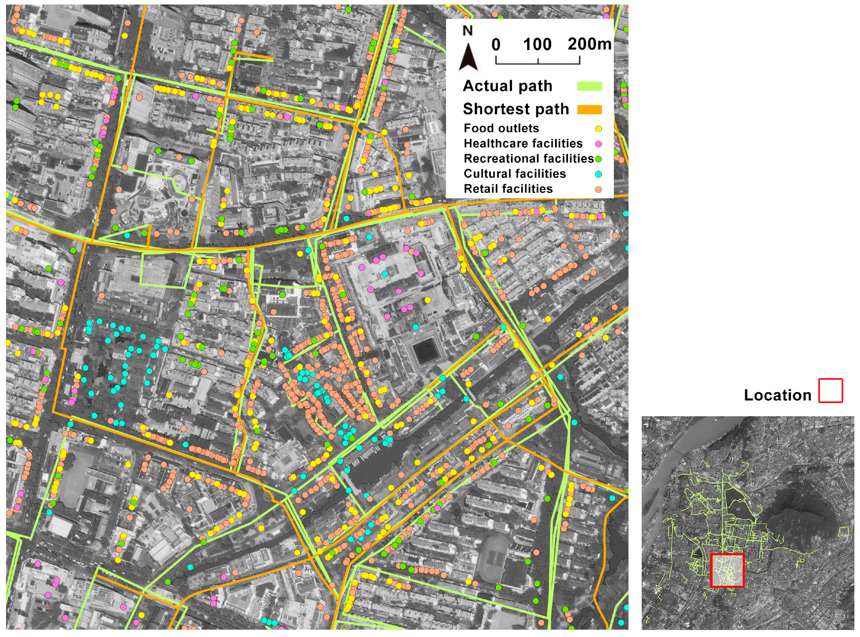
Distribution of POIs of various destinations.

Figure 7.
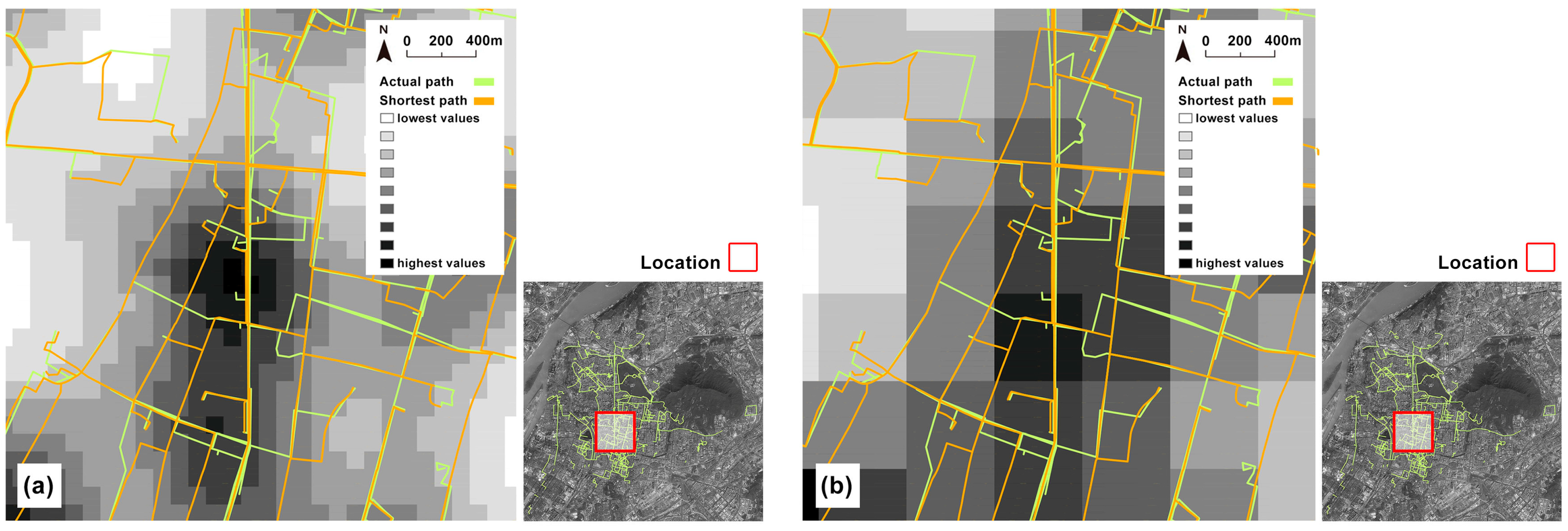
(a) Distribution of land-use mix at 100 m scale and (b) distribution of land-use mix at 500 m scale (results of Kernel density analysis).
Figure 7.
(a) Distribution of land-use mix at 100 m scale and (b) distribution of land-use mix at 500 m scale (results of Kernel density analysis).

Table 1.
The calculation method of built environment variables.
| Dimension | Environment Variables | Method |
|---|---|---|
| Density | Residential density | Total area of residential land within the buffer |
| Density | Building coverage | The ratio of the building footprint to the total area of the buffer zone |
| Density | FAR (floor area ratio) | The ratio of the floor area divided by the total area of the buffer zone |
| Density | Food outlets | Number of points of interest (POIs) of restaurants and cafes within the buffer zone |
| Density | Healthcare facilities | Number of POIs of pharmacies, health service centers, hospitals, and other types within the buffer zone |
| Density | Recreational facilities | Number of POIs of parks, bathing-massage, beauty salons, and karaoke within the buffer zone |
| Density | Cultural facilities | Number of POIs of buildings with historical and cultural significance, attractions, and memorials within the buffer zone |
| Density | Retail facilities | Number of POIs of shopping malls, shopping centers, supermarkets, stores within the buffer zone |
| Density | Industrial area | Total area of land with land use type of industrial land |
| Density | Commercial area | Total area of land with land use type of commercial land |
| Density | Administrative area | Total area of land with land use type of institutional land |
| Design | Intersection density | Number of road intersections divided by the area of the buffer |
| Design | Slope | Mean value of the slope raster within the buffer zone |
| Design | NDVI (normalized difference vegetation index) | Mean value of the NDVI raster within the buffer zone |
| Design | Water area | Total area of all waterbodies in the buffer zone |
| Design | Green area | Total area of green land within the buffer |
| Diversity | Land-use mix | The value of the mixed degree of land use of the buffer zone, calculated using the entropy approach [51]. The land use type includes five categories: residential land, industrial land, green area, commercial land, and institutional land. |
Table 2.
Descriptive characteristics of the participants (n = 105).
| Male | Female | Total | |
|---|---|---|---|
| All | 46 | 59 | 105 |
| Age 21–30 | 9 | 9 | 18 |
| Age 31–40 | 5 | 12 | 17 |
| Age 41–50 | 6 | 14 | 20 |
| Age 51–60 | 12 | 13 | 25 |
| Age 61+ | 14 | 11 | 25 |
Table 3.
Comparison of the length of the actual path and shortest path (m).
| MEAN | SD | |
|---|---|---|
| Actual path | 1707.13 | 2009.88 |
| Shortest path | 1366.03 | 1289.70 |
Table 4.
Mean differences in built environment characteristics along actual versus shortest routes (for other statistical variables, see Appendix A).
Table 4.
Mean differences in built environment characteristics along actual versus shortest routes (for other statistical variables, see Appendix A).
| MEAN | 50 m | 100 m | 200 m | 500 m | 800 m | 1600 m | ||||||
|---|---|---|---|---|---|---|---|---|---|---|---|---|
| Mean Diff | p-Value | Mean Diff | p-Value | Mean Diff | p-Value | Mean Diff | p-Value | Mean Diff | p-Value | Mean Diff | p-Value | |
| Residential Density | −61.7766 | 0.0014 ** | −170.1850 | / | −591.3204 | 0.0060 ** | −430.0442 | 0.6345 | −1863.7666 | 0.1572 | −5259.2856 | 0.0624 |
| Building Coverage | −0.0298 | 0.0000 ** | −0.0159 | 0.0000 ** | −0.0077 | 0.0081 ** | −0.0025 | 0.1653 | −0.0012 | 0.3921 | −0.0011 | 0.2697 |
| FAR | −0.1765 | 0.0000 ** | −0.1203 | 0.0000 ** | −0.0567 | 0.0192 * | −0.0284 | 0.0594 | −0.0124 | 0.3139 | −0.0101 | 0.2149 |
| Food Outlets | −0.0127 | 0.5370 | 0.0491 | 0.3575 | 5.4296 | 0.0000 ** | −0.2955 | 0.5888 | −1.5808 | 0.1600 | −2.7158 | 0.3645 |
| Healthcare Facilities | 0.0038 | 0.2695 | 0.0086 | 0.3776 | 0.0657 | 0.1036 | 0.0136 | 0.9280 | −0.1922 | 0.1861 | −0.1412 | 0.7694 |
| Recreational Facilities | 0.0173 | 0.0600 | 0.0573 | 0.0432 * | 0.1840 | 0.0187 * | −0.1427 | 0.6077 | −0.6645 | 0.2127 | −2.2127 | 0.1090 |
| Cultural Facilities | 0.0246 | 0.0000 ** | −0.0141 | 0.4018 | −0.0450 | 0.3241 | −0.1081 | 0.4610 | −0.2678 | 0.2103 | 0.1206 | 0.8092 |
| Retail Facilities | −0.0800 | 0.0605 | −0.1015 | 0.4811 | −0.2888 | 0.4143 | −1.3402 | 0.3032 | −4.3669 | 0.0612 | −8.0176 | 0.1568 |
| Industrial Area | −8.1237 | 0.1990 | −20.2899 | 0.3774 | −55.2679 | 0.4783 | −490.5920 | 0.3341 | 482.8308 | 0.3906 | −1529.9330 | 0.3941 |
| Commercial Area | −48.1754 | 0.0000 ** | −88.2299 | 0.0103 * | −83.6863 | 0.4651 | −579.7871 | 0.1925 | −1427.5869 | 0.0752 | −3222.9097 | 0.0658 |
| Administrative Area | −12.2204 | 0.1472 | −19.6496 | 0.5272 | 39.8189 | 0.7359 | 235.4142 | 0.6281 | 1135.6488 | 0.2833 | −2210.4884 | 0.2505 |
| Intersection Density | 0.0001 | 0.0000 ** | 0.0000 | 0.0000 ** | 0.0000 | 0.0000 ** | 0.0000 | 0.0078 ** | 0.0000 | 0.9582 | 0.0000 | 0.0046 ** |
| Slope | 0.0358 | 0.7115 | 0.1327 | 0.2289 | 0.1802 | 0.0954 | −0.0629 | 0.6284 | 0.1530 | 0.1351 | 0.0565 | 0.5482 |
| NDVI | −7.9588 | 0.1460 | −148.8251 | 0.0000 ** | 429.2692 | 0.0000 ** | 273.0531 | 0.0165 * | 179.1272 | 0.1367 | 95.1563 | 0.3945 |
| Water Area | −0.1065 | 0.9713 | 2.1019 | 0.8748 | 3.6390 | 0.9512 | −119.3293 | 0.7138 | −530.3960 | 0.5163 | −1162.7928 | 0.6305 |
| Green Area | −7.6143 | 0.5195 | 6.7490 | 0.8674 | 49.1808 | 0.6793 | 586.4563 | 0.1827 | 638.5980 | 0.4757 | 3216.8065 | 0.2445 |
| Land-Use Mix | −0.0078 | 0.0641 | −0.0024 | 0.5345 | 0.0022 | 0.5091 | −0.0029 | 0.3418 | −0.0005 | 0.8037 | −0.0049 | 0.0033 ** |
(Mean diff = Shortest Route-Actual Route). ** Significant at 0.01 level, * significant at 0.05 level.
Disclaimer/Publisher’s Note: The statements, opinions and data contained in all publications are solely those of the individual author(s) and contributor(s) and not of MDPI and/or the editor(s). MDPI and/or the editor(s) disclaim responsibility for any injury to people or property resulting from any ideas, methods, instructions or products referred to in the content. |
© 2023 by the authors. Licensee MDPI, Basel, Switzerland. This article is an open access article distributed under the terms and conditions of the Creative Commons Attribution (CC BY) license (https://creativecommons.org/licenses/by/4.0/).
Share and Cite
MDPI and ACS Style
Ge, Y.; He, Z.; Shang, K. Influence of the Built Environment on Pedestrians’ Route Choice in Leisure Walking. ISPRS Int. J. Geo-Inf. 2023, 12, 384. https://doi.org/10.3390/ijgi12090384
AMA Style
Ge Y, He Z, Shang K. Influence of the Built Environment on Pedestrians’ Route Choice in Leisure Walking. ISPRS International Journal of Geo-Information. 2023; 12(9):384. https://doi.org/10.3390/ijgi12090384
Chicago/Turabian StyleGe, Yifu, Zhongyu He, and Kai Shang. 2023. "Influence of the Built Environment on Pedestrians’ Route Choice in Leisure Walking" ISPRS International Journal of Geo-Information 12, no. 9: 384. https://doi.org/10.3390/ijgi12090384
Note that from the first issue of 2016, this journal uses article numbers instead of page numbers. See further details here.