

Gated Recurrent Unit Embedded with Dual Spatial Convolution for Long-Term Traffic Flow Prediction

School of Automation, Wuhan University of Technology, 122 Luoshi Road, Wuhan 430070, China
*
Author to whom correspondence should be addressed.
†
These authors contributed equally to this work.
ISPRS Int. J. Geo-Inf. 2023, 12(9), 366; https://doi.org/10.3390/ijgi12090366
Submission received: 27 June 2023
/
Revised: 27 August 2023
/
Accepted: 30 August 2023
/
Published: 5 September 2023
(This article belongs to the Topic Geocomputation and Artificial Intelligence for Mapping)
Abstract
:Considering the spatial and temporal correlation of traffic flow data is essential to improve the accuracy of traffic flow prediction. This paper proposes a traffic flow prediction model named Dual Spatial Convolution Gated Recurrent Unit (DSC-GRU). In particular, the GRU is embedded with the DSC unit to enable the model to synchronously capture the spatiotemporal dependence. When considering spatial correlation, current prediction models consider only nearest-neighbor spatial features and ignore or simply overlay global spatial features. The DSC unit models the adjacent spatial dependence by the traditional static graph and the global spatial dependence through a novel dependency graph, which is generated by calculating the correlation between nodes based on the correlation coefficient. More than that, the DSC unit quantifies the different contributions of the adjacent and global spatial correlation with a modified gated mechanism. Experimental results based on two real-world datasets show that the DSC-GRU model can effectively capture the spatiotemporal dependence of traffic data. The prediction precision is better than the baseline and state-of-the-art models.
1. Introduction
AS people’s standards of living improve, their desire for a better life becomes increasingly strong. The convenience of commuting and traveling attracts more and more families to choose cars as their mode of transportation. In most cities across the country, road occupancy rate continues to increase. while the average driving speed during rush peak hours has sustained a decrease. This leads to the deterioration of urban road operations. In this case, not only the efficiency of urban road use will be significantly reduced but also fuel cannot be completely burned when cars drive at a low speed. This shortens the service life of the engine and produces a lot of harmful gas pollution, both of which increase the cost of car maintenance and environmental management [1]. As an integral component of an Intelligent Transportation System (ITS), how to improve the accuracy of traffic flow prediction and use it as the basis for rational route planning to reduce road congestion has emerged as a research focal point [2].
In order to enhance the precision of traffic flow prediction, many scholars in the field of traffic flow prediction have proposed various prediction models in recent years. These models for predicting traffic flow can be generally categorized into three groups, including statistical analysis models, machine learning models, and deep learning models. Statistical analysis models commonly used in traffic flow prediction include the Historical Average model(HA) [3], the Autoregressive Integrated Moving Average model(ARIMA) [4], and the Kalman filtering model [5]. These models can achieve better results when dealing with static data. However, traffic flow data change dynamically over time and have strong spatial dependence. Statistical analysis methods are insensitive to these types of data; so, these models often fail to achieve the desired results when performing traffic flow prediction tasks [6]. Machine learning models for traffic flow prediction are introduced to solve the above problem, such as the K-Nearest Neighbor model (KNN) [7], the support vector regression model [8], and the Bayesian network model [9]. For the sake of achieving superior predictions from machine learning models, it is necessary to set appropriate parameters for the models based on a large amount of a priori knowledge. It is difficult and laborious to set the optimal hyperparameters of the model artificially; so, the power of the model is often not fully exploited. As artificial intelligence is increasingly applied to various fields, deep learning is receiving more and more attention. Deep-learning-based traffic flow prediction models stack multiple layers of neural network to capture various dependence of the traffic data. The effect of hyperparameters is weakened [10], and the influence of human factors is reduced [11]. For example, recurrent neural networks (RNNs) [12] and their variant long short-term memory (LSTM) [13], as well as Gated Recurrent Units (GRUs) [14], have achieved great results in performing temporal features extraction [15]. Graph convolutional networks (GCNs) [16], which evolved from convolutional neural networks (CNNs) [17], are commonly used for learning the temporal features of traffic data.
The main challenges of traffic prediction task originate from the spatial and temporal dependencies inherent in traffic flow data [18]:
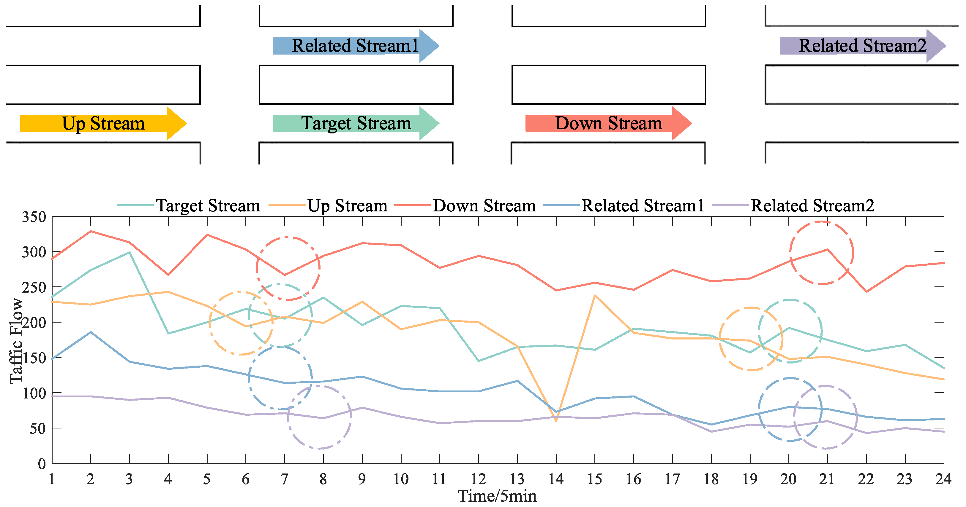
(1) Spatial dependence: The layout of the nodes in the urban road network is generally an irregular graphical topological structure, as shown as Figure 1.
Such a spatial structure will make the traffic state between the nodes interfere with each other. The traffic state of upstream and downstream nodes in the same segment has different effects on the target node [19]. It is also found that even if the node is far from the target node in the road network space, it will affect the prediction of future traffic flow at the target node [20]. As shown in Figure 1, it can be observed that certain segments of the time series share similar trends, as indicated by the circled areas. Additionally, both upstream and downstream traffic flow data exhibit similar patterns, albeit with a delay in the downstream traffic flow changes. This suggests a correlation between the two types of traffic flow and a potential lag effect in the downstream traffic flow. Moreover, these nodes with high spatial correlation have some kind of correlational relationship or common influencing factors that lead to changes in traffic status with similar trends (e.g., Related Stream). How to exploit the existing relationship between spatial nodes is important to improve the accuracy of traffic flow prediction.
(2) Temporal dependence: Temporal modeling of traffic flow data requires consideration of the inherent properties of traffic flows.
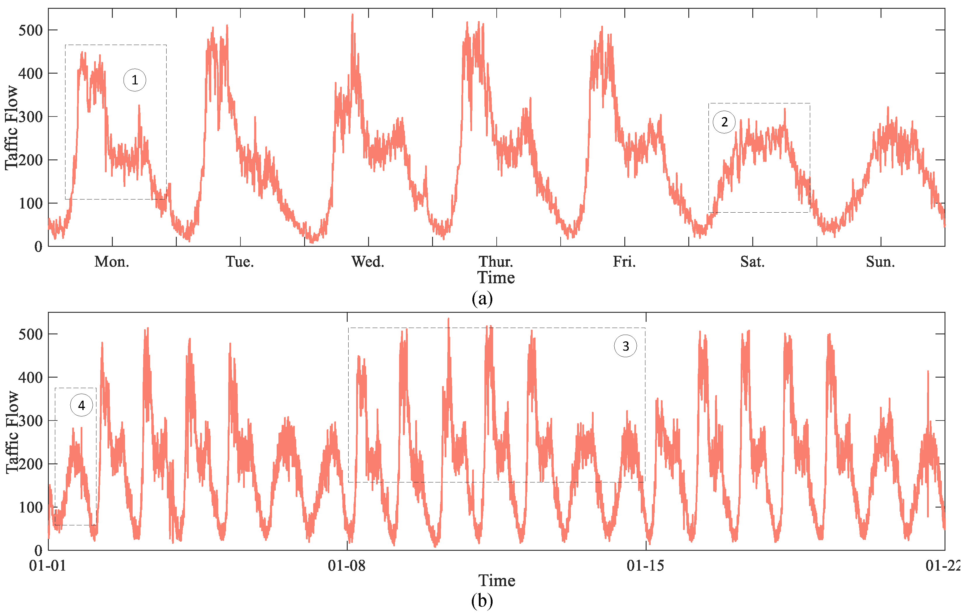
The traffic flow data of each node in the urban road network vary dynamically and periodically with time [21]. Meanwhile, traffic flow data at urban road network nodes can also be subject to many uncertainties (e.g., weather, traffic accidents, etc.) [22].
Figure 2, where ①, ②, ③, and ④ represent the traffic flow data of one workday, weekend, holiday, and week, respectively, demonstrates that the traffic flow data have the following characteristics in the time dimension. First, traffic flow data have obvious daily periodicity (e.g., ① and ②) and weekly periodicity (e.g., ③), and the change pattern of weekdays is significantly different from that of weekends. Second, since the change pattern of traffic data on holidays is different from that of weekdays, it will break the periodicity of traffic state change (e.g., ④). To meet the requirement of prediction accuracy, the above dynamic change patterns must be fully considered.
To address the challenges in traffic flow prediction, the main contributions of this work are as follows:
(1) We propose a new traffic flow prediction model, termed Dual Spatial Convolution Gated Recurrent Unit (DSC-GRU), which considers the spatiotemporal dependence of the traffic flow data and achieves a more accurate prediction result.
(2) Based on the R-Square (), we design a correlation matrix that reflects whether the nodes are spatially related or not, allowing the graph convolution network to be aware of global features, and develop a gated-mechanism-based spatial graph convolution module that integrates the neighborhood and global features through a learnable parameter matrix.
(3) The proposed model is capable of synchronously incorporating both temporal and spatial correlations of traffic flow data. This capability is achieved by embedding a Dual Spatial Convolution (DSC) module into the GRU architecture. The DSC facilitates the integration of spatial information into the state of the GRU without compromising its ability to learn the complex temporal dynamics of the traffic flow data.
Our model is evaluated on two real-world traffic datasets. Compared with the baseline and state-of-art models, the results show that the DSC-GRU outperforms all of them.
The rest of this paper is organized as follows. Section 2 presents related work and introduces various existing models used for traffic flow prediction; Section 3 is the problem description, which defines the traffic flow prediction problem; Section 4 is the methodology, which presents the details of the proposed model; Section 5 is the experimental setting, which presents the relevant details of the experiments; Section 6 is the experimental results and analysis, and it visualizes the results; and Section 7 concludes the whole paper.
2. Related Work
Facing the high-dimensional temporal data of traffic flow, the performance of traditional statistical analysis models and machine learning models are increasingly unable to meet the accuracy requirement of traffic flow prediction. Meanwhile, with the improvement of information collection technology and computer processing power, many researchers have turned their attention to deep-learning-based traffic flow prediction methods [23].
Deep learning methods commonly used in traffic flow prediction can be broadly classified into two categories: temporal feature extraction models and spatiotemporal feature extraction models.
(1) Temporal feature extraction model:
A fundamental feature of time series data is that data at historical moments will affect the pattern of data changes at future moments. Wang et al. [24] designed a traffic flow prediction model based on back propagation neural network. The predicted value is obtained after a series of nonlinear variations in the input data. Huang et al. [25] proposed the deep belief network model, consisting of a deep belief network for unsupervised traffic flow feature learning and a multitasks regression layer for supervised prediction. Lv et al. [26] used a stacked autoencoder to learn traffic flow features, and it was trained bottom-up layer by layer with the greedy wolf algorithm. Logistic regression was used to complete the traffic flow prediction task. These models ignore the sequential relationship in the time series. The output corresponding to the input of each moment is not affected by the previous input. As a result, the prediction accuracy of these models is not satisfactory. To consider the sequential relationship of time series data, RNNs have been proposed. As a classical model for time series processing, RNNs can handle the sequential relationship in the time series. However, they have some defects, such as gradient disappearance and gradient explosion. Many improvements on RNN models have overcome the above problems and achieved better results in time series prediction, such as Ma et al. [27], who were the first to apply LSTM to traffic flow prediction. The error decay problem in the backpropagation process has been overcome. Sun et al. [28] stacked multiple GRUs to enhance the ability to extract the temporal features. In addition, the Seq2Seq model provided a novel idea for traffic flow prediction. The Seq2Seq model was first proposed to solve the machine translation problem [29]. Sutskever et al. [30] created an end-to-end sequence learning method based on the Seq2Seq model. The encoder and decoder are formed by stacking multilayer LSTMs. The encoder encodes the input sequence into a vector of fixed dimensions, and the decoder subsequently decodes the vector to obtain the target sequence.
(2) Spatiotemporal feature extraction model:
With the iterative upgrade of deep learning techniques, researchers increasingly feel that simple time series prediction models cannot meet the accuracy requirement of traffic flow prediction task. Since the topological structure of the road network affects the traffic state of the nodes, researchers have begun to turn their attention to prediction models with the fusion of spatiotemporal features [31]. CNNs point the way to learning spatial features for traffic flow prediction models [32]. The ConvLSTM model created by Shi et al. [33] combined a CNN with LSTM for the first time to address the prediction problem. The CNN can handle the graph structure of Euclidean space well, but it is hard for it to process the graph structure of the road network, which belongs to non-Euclidean space. The GCN was raised to map the traffic road network to Euclidean space for processing. Zhao et al. [34] designed a Temporal Graph Convolutional Network (T-GCN) which used the GCN model to learn the complex spatial topological structure in the road network space and used GRU to obtain the time dependence of the traffic data. The attention mechanism is also widely used in traffic flow prediction tasks. Guo et al. [35] proposed the attention-based spatiotemporal graph convolutional network. The attention mechanism is introduced to model three types of temporal dependence. Much research has been conducted to overcome the drawback that the GCN can only consider the information of adjacent nodes and give equal weight to neighboring nodes. Huang et al. [36] developed a diffusion convolutional recurrent neural network model to integrate the information of all nodes within n-hops by means of random wandering. Bao et al. [37] designed a spatial–temporal complex graph convolution network which considers the influence of external factors such as weather and facilities around the nodes. Wu et al. [38] raised the Graph WaveNet. The adaptive dependency matrix is used to capture the temporal dependence accurately. Song et al. [39] designed a spatiotemporal synchronous modeling mechanism to effectively capture the complex localized spatiotemporal dependence. The improvements on the road network graph structure have become the mainstream methods to capture the spatial dependence of traffic data.
Motivated by the above method, the correlation matrix is designed to learn the global spatial dependence of the traffic data, which enhances the spatiotemporal feature capturing ability of our proposed DSC-GRU model.
3. Problem Description
The traffic flow prediction task aims at predicting the traffic state of the urban road network at a future moment using historical traffic flow data [40]. Traffic flow data includes vehicle speed, traffic flow, and road network density [41]. In this study, we use traffic flow as an example to elaborate the model.
Traffic road network: The road network is used to describe the spatial topology structure of the urban road network. denotes the set of road network nodes, and is the number of nodes. Since the graph used in our model is an undirected graph, is the set of edges connected by any two road network nodes.
Feature matrix: The traffic flow data , where represents the length of the time series collected at each node; then, the traffic flow data at the time is . Based on the above definitions, the traffic sequences input to the model and the predicted sequences output from the model are given as and , respectively, where denotes the length of the historical time series used for prediction, and represents the size of the predicting window.
Mapping function: The traffic flow prediction task can be described as a process of training a mapping function from input to output, which takes historical traffic flow data with known graph structures G as input and calculates the traffic flow values in the following moments, as shown in Equation (1).
4. Methodology
This section explains how the DSC-GRU model can consider spatiotemporal features and complete the traffic prediction task.
4.1. Overview
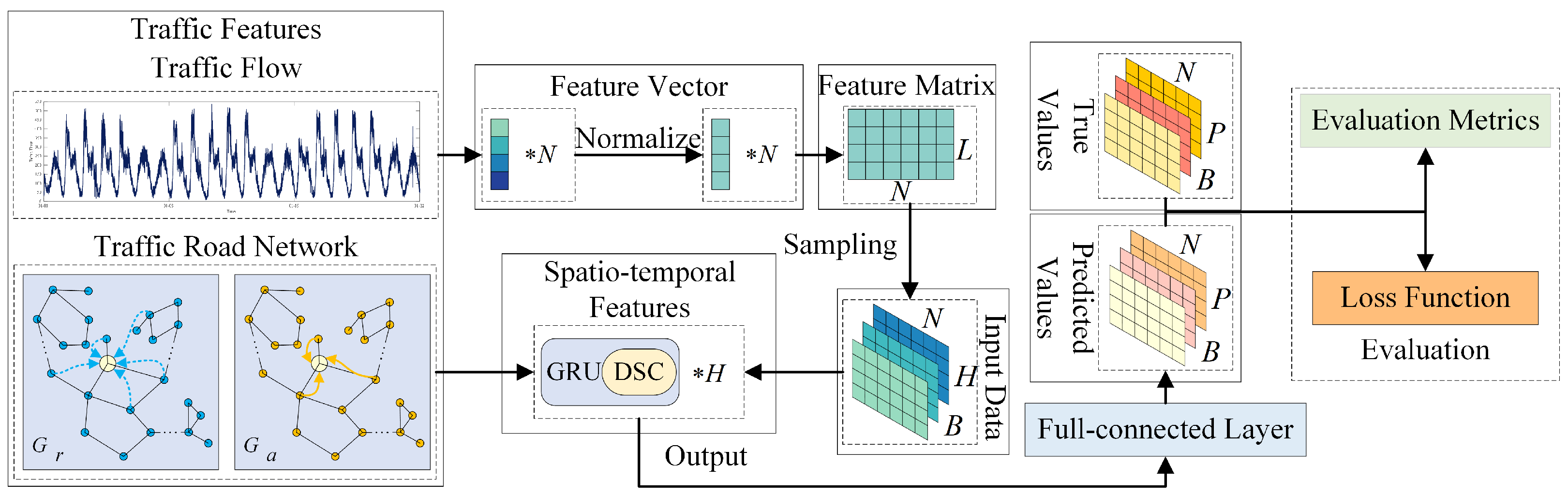
The DSC-GRU model consists of a GRU embedded with a DSC. The framework of our proposed model is shown in Figure 3, where B, H, and P represent the batch size of data used to train the prediction model once, the length of the input model’s historical data, and the length of the model’s output prediction data, respectively. And sampling refers to dividing the feature matrix into a number of H-length matrix blocks along the L dimension and randomly selecting the B-matrix blocks as the input data to the model for a training epoch.
Based on the existing graph structure and , the DSG-GRU model is used to extract the spatial and temporal features of the traffic flow data. The DSC-GRU model retains the ability of the GRU to extract dynamic time series features. The embedded DSC is used to obtain the spatial topological structure of the urban road network, thus capturing the spatial characteristics of the traffic data. Finally, the output prediction results are obtained through a fully connected layer.
The core ideas of the DSC-GRU can be summarized into three aspects: (1) Spatial correlation matrix: design a correlation matrix based on the correlation coefficient to learn the spatial correlation of the traffic road network. (2) Spatial features fusion: a gated mechanism is introduced to integrate adjacent features and global features of the traffic road network to optimize the prediction performance of the network. (3) Temporal features extraction: adopt the GRU network to capture the temporal correlation of the traffic flow data.
4.2. Spatial Dependence Modeling
Obtaining the spatial features of urban road network is a critical problem that has long plagued traffic flow prediction. Although CNN models can capture spatial features in Euclidean space well, the complex topological structure of urban road network belongs to non-Euclidean space, so CNNs cannot accurately capture the spatial dependencies of traffic data [42]. In recent years, the GCN model, which evolved from CNNs, has been widely used in computer vision [43], biochemistry [44], and other fields with good results due to its great ability to handle various graph structures.
4.2.1. Graph Data Definition
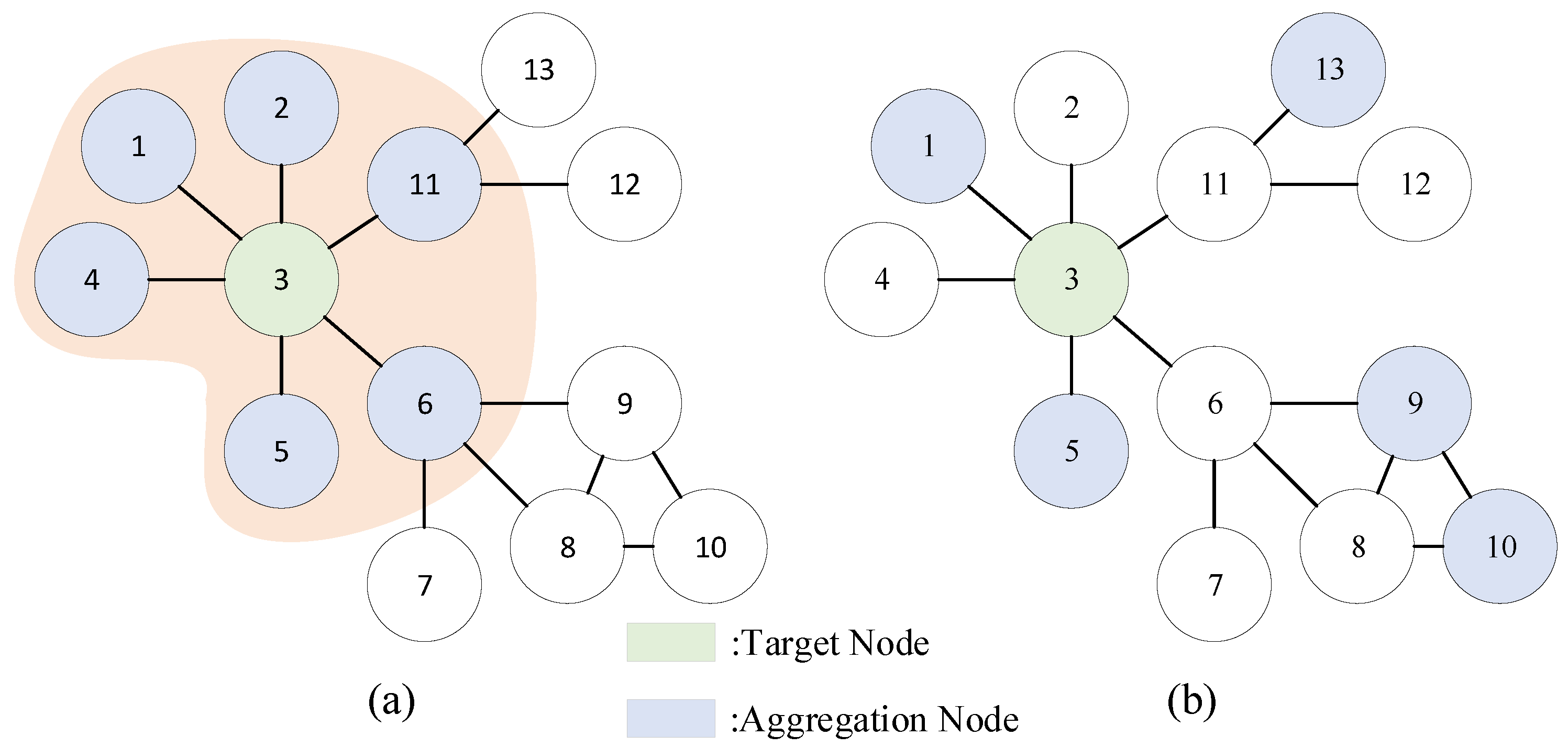
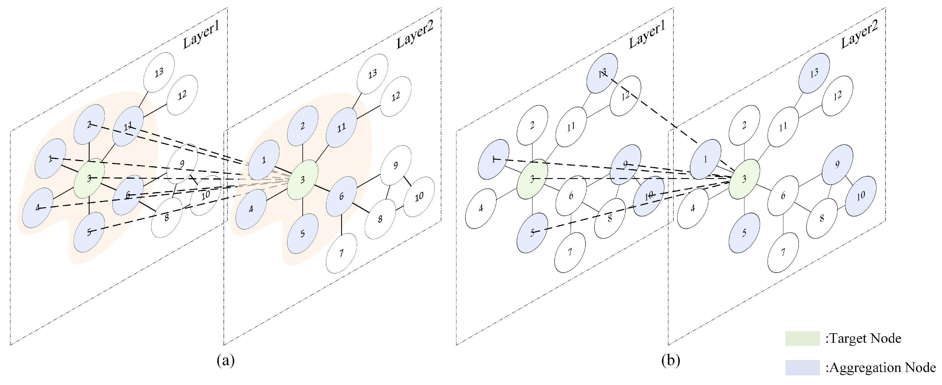
In order to more accurately capture the spatial dependencies in traffic flow data, the GCN model maps the spatial topology of the traffic road network from a non-Euclidean space to a Euclidean space. However, our proposed model involves two distinct scales of spatial structures; so, it is necessary to define the spatial structure graph data separately. Figure 4a,b show the distribution of aggregation nodes in the adjacency graph and the global graph, respectively.
The adjacency graph, which is mapped to Euclidean space to obtain the adjacency matrix , characterizes the spatial structure of adjacent nodes. The adjacency matrix denotes that the connection relationship in the set of edges E is defined in Equation (2),
where represents node i connected to node j and vice versa.
The adjacency matrix used in traditional graph convolution can generally only aggregate the spatial structure within the adjacent nodes or n-hop nodes of the road network. These simple graphs are based on the assumption that the upstream and downstream traffic states on the same road section have a strong influence on the traffic state of the target node, which neglect the topological structure of the whole urban road network.
In order to obtain the spatial feature of the whole road network, some studies used the KNN [45] algorithm to calculate the correlation between the two time series so that the topological structure of the urban road network can be fully explored. The KNN algorithm selects nodes with the highest relevance to the target node in the entire road network. It may happen that nodes are not actually strongly correlated but are identified as strongly correlated by the KNN algorithm. From such nodes, the model will learn a lot of useless information.
To make spatial information aggregation more flexible and accurate, the correlation coefficient is introduced to quantify the correlation between different nodes. The is derived as follows:
where SST, SSR, and SSE refer to Sum of Squares Total, Sum of Squares Regression, and Sum of Squares Error, respectively, represents the correlation between the node and the node , the value closer to 1 means the greater correlation, and and represent the traffic flow value and the average traffic flow value of the node at the time , respectively. The relationship between the correlation coefficient and correlation strength is shown in Table 1 below.
The correlation of road network nodes is calculated based on the correlation coefficient. It is assumed that if the correlation coefficient exceeds the threshold, then the corresponding nodes are considered to be strongly correlated. On this basis, is defined as Equation (7),
where means that the corresponding node is highly correlated and vice versa.
4.2.2. Graph Data Processing
The graph structure used in most traffic flow prediction task is often an undirected graph based on the urban road network. In this case, the GCN network integrates the characteristics of the nodes and their neighbors based on the weight matrix and the adjacency matrix . The GCN network contains a two-layer structure, which is calculated as shown below:
where and are the weight matrices of the first and second layer GCN network, respectively.
Adjacency matrix is defined to merge the node’s own information,
where is an identity matrix with the same dimension as the number of nodes, and is the weight factor and takes a value of 1, indicating that the information of this node is as important as that of its neighbors.
The GCN model normalizes the rows and columns of the adjacency matrix by the symmetric normalized Laplacian matrix,
where the degree matrix is the diagonal matrix, is the element on the degree matrix, and represents the element of the row and column of the matrix .
In summary, the standard format of the GCN network can be described as the following equation:
By replacing the adjacency matrix A in the traditional GCN network with the adjacent matrix and correlation matrix , the topological structure information of the adjacent space and global space can be integrated.
4.2.3. Dual Spatial Convolution
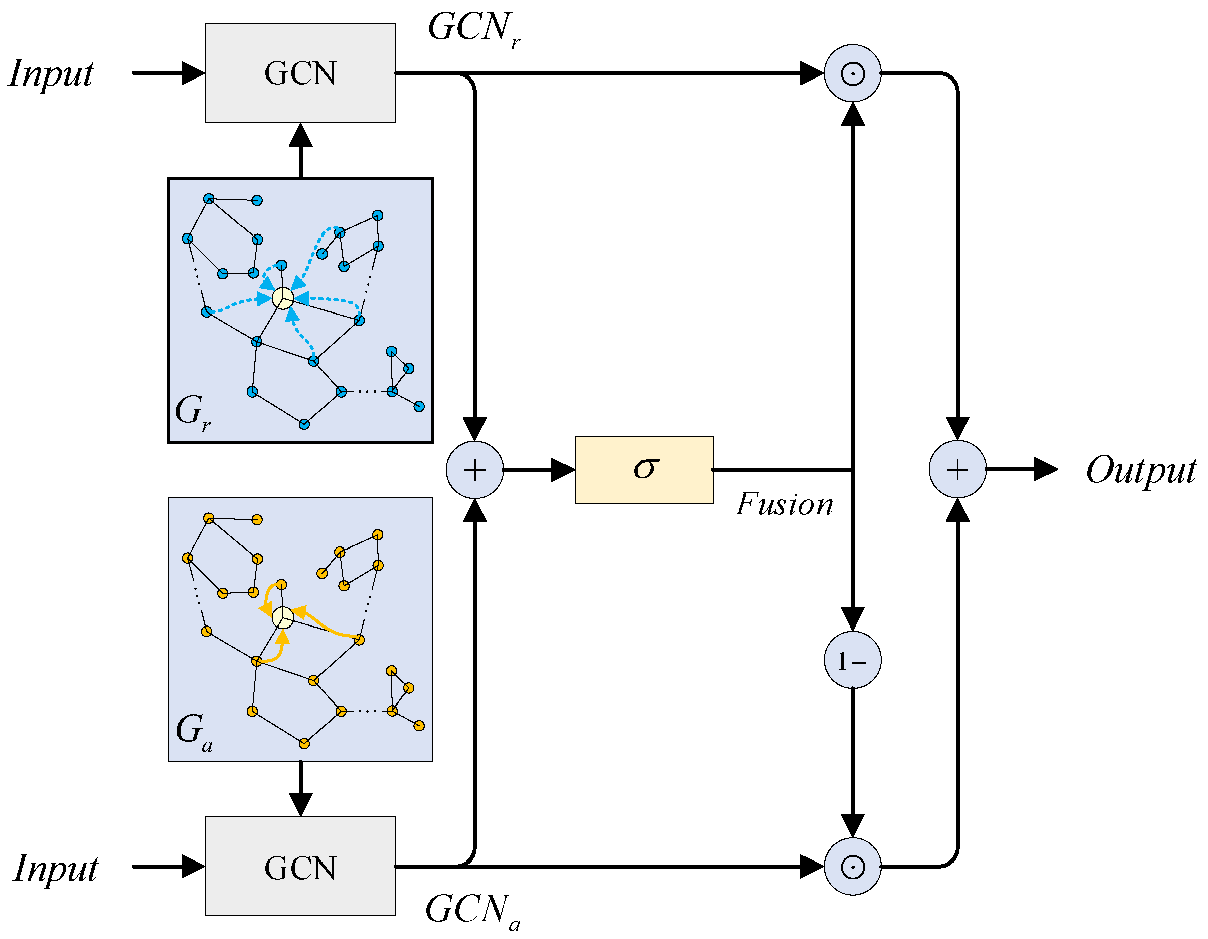
The process of integrating the structural information of the adjacent space and the global space is shown in Figure 5a,b, respectively.
If the adjacent and global information are simply superimposed, it must be assumed that their importance is equal. However, it is impossible to artificially judge the significance of the adjacent and the global information in the traffic flow prediction task. A simple superposition will seriously reduce the prediction accuracy of the model. The role of the gated mechanism is that the learning of the weight matrix can adjust the importance of the adjacent information and the global information to the target node to achieve better prediction accuracy.
In addition, there is a particular case if the calculated correlation between the target node and its neighbor exceeds the set threshold. The information of those neighbor nodes will also be fused when integrating global information. To some extent, it alleviates the problem that the traditional graph convolution model ignores the differences in the influence of different neighborhoods on the target node.
The output of the graph convolution operation for and is recorded as and , respectively. They are used as the inputs to the gated unit. The overall structure of the DSC is shown in Figure 6, where “⊕” and “⊙” represent the addition and multiplication of the corresponding elements of the isotype matrix, respectively, and “” means 1 minus the elements of each position of the matrix. represents the sigmoid activation function, which maps the input to the [0, 1] interval. Its forward propagation equations are shown as Equations (13)–(16):
where W and b are the parameter matrix, represents the output of the DSC unit, and incorporates the spatial information of the adjacent space and the global space. is used to adjust the proportion of the importance of the global information. The closer to 1, the higher the importance of the global information. Then, there is more focus on the spatial information of the whole road network space when performing the prediction task and, conversely, focus on the spatial information of the adjacent space.
In summary, the DSC can balance the relative importance relationship between the adjacent space and the global space through the gated mechanism. This allows the DSC to better extract the topological structure of the urban road network and capture the spatial dependence of traffic data.
4.3. Spatiotemporal Dependence Modeling
In the previous subsection, we used the DSC to extract the spatial dependence of traffic data. Still, another critical issue in the traffic flow prediction task is extracting time series features. The most commonly used method for processing time series data is the RNN, and it achieves promising results on many models. Due to the defects of gradient explosion and gradient disappearance, traditional RNNs cannot obtain the temporal features of traffic flow data, which has long-term time-dependent data. The LSTM and the GRU are proposed as variants of the RNN. They provide solutions to the above problems. The principles of the LSTM and the GRU are similar [46]. Both are based on RNNs and add a gating mechanism and long-term information memory cells, thus solving the problem of long-term dependence on time series.
Compared with LSTM, GRUs have fewer parameters, require less computational power, and are easier to converge during the training process with less risk of overfitting. Therefore, the spatiotemporal dependence is modeled based on the GRU framework in this paper.
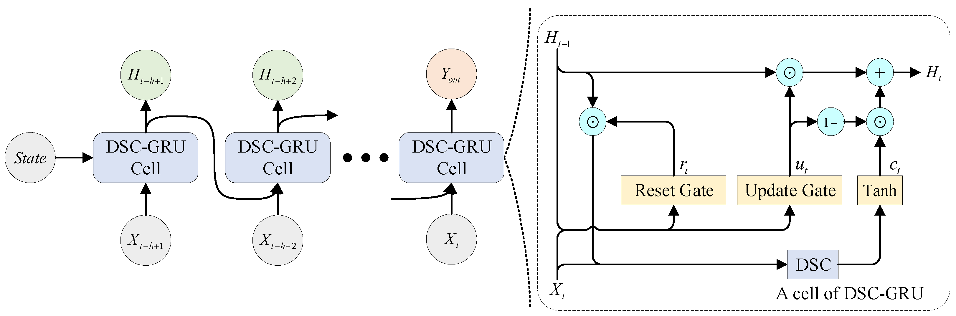
In order to obtain both the temporal-dependent and spatial-dependent traffic flow data, the DSC-GRU traffic flow prediction model is proposed by embedding the DSC into the framework of GRU. The overall prediction process of the DSC-GRU model is shown in Figure 7, where represents the hidden layer state output by the DSC-GRU cell at the time step t, and is the final result of the DSC-GRU cell output. , , and are the calculation results of the reset gate, the update gate, and the candidate hidden state at the time step t, respectively. The left side is the schematic diagram of the forward propagation of the model, and the right side is the specific structure of the DSC-GRU.
The DSC-GRU model forward propagation is formulated as Equations (17)∼(20):
where W, b is the parameter matrix of each state in the training process, has the same meaning as the previous section, represents the tanh activation function, which maps the input to the [−1, 1] interval to prevent the gradient explosion due to the large number of parameters in the backpropagation process, and denotes the result obtained by DSC cell calculation.
The DSC-GRU model retains the ability of the GRU model to capture the long-term dependence of the time series by processing the input at the moment t and the hidden state at the previous moment. The temporal information of the current moment and the historical moment are fused. The dynamic characteristics of the time series are preserved. On this basis, the DSC unit is embedded to capture the spatial dependence of the traffic data. The validity fraction of the historical spatiotemporal information is obtained through reset gates and passed to the next moment. On the moment t, the input hidden layer state of the DSC-GRU model already contains both temporal and spatial information from the previous moment. The DSC fuses valid historical spatiotemporal information with the input of the current moment. On the one hand, the spatial features of the current input data are fused. On the other hand, the importance of spatial features in historical information is strengthened. Up to this point, the embedding of the DSC has added the spatial information of the urban road network to each state in the GRU model. This spatial information is passed from the previous time step to the next time step as the GRU model passes temporal information. Throughout the forward propagation process, the above operation is repeated several times to continuously reinforce the learning of spatial features by the DSC to improve the model’s ability to extract spatial dependencies. The pseudocode of the model is shown in Appendix A.
In summary, the DSC-GRU model can explore the hidden spatial dependence and temporal dependence of traffic flow data. For one thing, the DSC unit is used to obtain the topological structure of the whole urban road network and then obtain the spatial dependence of the traffic flow data. For another, the GRU model is used to obtain the temporal dependence of traffic flow data by considering the long-term temporal relationship in traffic flow data. Finally, the task of traffic flow prediction is completed.
5. Experiment Setting
In order to verify the effectiveness and generalization ability of the traffic flow prediction model proposed in this paper. The prediction performance of the DSC-GRU model is evaluated based on two real datasets, and the results are visualized.
5.1. Data Description
In this paper, the PeMS04 and PeMS08 datasets are used to evaluate model performance. Both of them are highway datasets collected by the California Department of Transportation based on the Caltrans Performance Measurement System (PeMS). The system collects real-time traffic status at 30 s intervals and aggregates all information collected at 5 min intervals. All datasets contain three characteristics dimensions: vehicle speed, traffic flow, and network density. In this paper, the traffic flow is used as the research object. The training set, validation set, and test set are divided in the ratio of 6:2:2. The differences between PeMS04 and PeMS08 are as follows:
(1) PeMS04: This dataset contains a total of 307 road nodes. It was collected for 59 days from 1 January 2018 to 28 February 2018, of which 35 days were used as the training set, 12 days as the validation set, and 12 days as the test set.
(2) PeMS08: This dataset contains a total of 170 road nodes. It was collected for 62 days from 1 July 2016 to 31 August 2016, of which 38 days were used as the training set, 12 days as the validation set, and 12 days as the test set.
5.2. Evaluation Metrics
The predictive performance of our DSC-GRU model is evaluated by the following four evaluation metrics.
(1) Mean Absolute Error (MAE):
(2) Root Mean Squared Error (RMSE):
(3) Mean Absolute Percentage Error (MAPE):
(4) Coefficient of determination ():
where and represent the real traffic state and predicted traffic state of node i at the time j, respectively, is a subsidiary term, and is the average value of traffic flow data. MAE and RMSE are used to measure the degree of deviation of the model’s predicted value from the true value. MAPE indicates the relative size of the deviation of the model’s predicted value from the true value. weighs the ability of the model’s predicted value to represent the true value. The smaller the MAE, RMSE, and MAPE and the larger the , the better the prediction performance of the model.
5.3. Loss Function
The goal of training the traffic flow prediction model is to minimize the deviation of the predicted value from the true value of the traffic flow data, i.e., to minimize the value of the loss function. The loss function used to train this model is shown in Equation (25),
where y and represent the true value and predicted value of traffic flow, respectively. The default value for takes 1.
The advantage of this type of loss function is that the curve is relatively smooth. When the difference between the predicted value and the true value is slight, the gradient will not be too small. When the difference is significant, it is not easy for gradient explosion to appear.
5.4. Parameter Setting
The parameters of the DSC-GRU model include batch size, learning rate, number of iterations, threshold, historical data length h, prediction length p, and the number of neurons in the DSC and the GRU hidden layer ( and ). In the experimental process, the batch size is set to 64, the learning rate is set to 0.002, the number of iterations is set 2000, and the h and p are set to 12, i.e., the historical information of the past hour is used to predict the traffic flow of the future hour. Furthermore, threshold, , and are set to 0.8, 512, and 128, respectively.
In addition, a variable learning rate mechanism is introduced for better learning of traffic flow data. When the current optimal value does not appear in 10 consecutive training epochs, the learning rate of the model is considered too large, and the network hovers around the optimal value. The learning rate is reduced to the original 0.1 so that the model can learn more carefully. When the current optimal value appears, the learning rate is reset to 0.002 to make the model converge quickly in the new solution space. And random seeds are set in the same group of experiments to ensure the same initialization parameters of the model and reduce the effect of random errors.
5.5. Compared Methods
In order to verify the validity and the advancement of the proposed model, the model is compared with five baseline models considering a single feature of the traffic flow data as well as two spatiotemporal models proposed in recent years. These methods are as follows:
(1) HA [3]: The average value of historical traffic flow data is used as the traffic flow prediction for the next moment.
(2) ARIMA [4]: Traffic flow data are considered as a time series with seasonal patterns. It is possible to separate the signal from the noise and obtain predicted values by extrapolating the signal to the future.
(3) LSTM [27]: One of the variants of the recurrent neural network, which obtains long-term dependencies in the time dimension by introducing a gated mechanism. It can solve the problem of gradient disappearance and gradient explosion in traditional recurrent neural networks.
(4) GRU [28]: The principle is similar to that of LSTM, except that the number of parameters in the training process is smaller and the computation is simpler.
(5) GCN [16]: Mapping the road network space from non-Euclidean space to Euclidean space. The spatial features of traffic data are extracted from neighboring nodes in the traffic road network.
(6) T-GCN [34]: Combines the advantages of both the GCN and the GRU, which consider the temporal dependence and spatial dependence of traffic data.
(7) Graph WaveNet [38]: The adaptive dependency matrix and the dilated convolution structure are designed to accurately capture the spatiotemporal dependencies in traffic flow data.
6. Experiment Result and Analysis
This section tests the prediction performance of the DSC-GRU model by setting comparison experiments, different thresholds, structural parameters, and ablation experiments.
6.1. Comparison Experiments
The performance of the different models is shown in Table 2, where the bolded parts are the models proposed in this paper. It is shown that the DSC-GRU model outperformed all comparison models on the four evaluation metrics.
The experiment results are analyzed in four aspects, as follows. Initially, the reason why the statistical analysis models (HA and ARIMA) perform worse than the deep learning models is that these models are insensitive to the dynamically changing traffic flow data and cannot explore the spatial information of the traffic data. Secondly, either the deep learning models that consider only temporal dependence (LSTM and GRU) or those that consider only spatial dependence (GCN) do not achieve satisfactory prediction results. The reason is that the traffic data are essentially time series data, which are influenced by the topological structure of the road network. Neglecting either the temporal or the spatial dependence will lead to a decrease in prediction accuracy. Thirdly, the spatiotemporal characteristics models (T-GCN and Graph WaveNet) have significantly better prediction performance than the LSTM, GRU, and GCN. The improvement in the prediction performance results from these models taking the spatiotemporal dependence of traffic flow data into consideration rather than single dependence. This demonstrates that the spatiotemporal dependence of the traffic data is of great importance for improving prediction accuracy. Finally, the DSC-GRU model proposed in this paper also considers the spatiotemporal dependence of traffic flow data simultaneously. As opposed to the above spatiotemporal models that only consider the spatial characteristics of nodes within a certain range, the DSC-GRU model can capture the global spatial characteristics of nodes. Therefore, the prediction performance is better than that of the T-GCN and Graph WaveNet models. Specifically, compared with the T-GCN and Graph WaveNet, the MAE value is decreased by 10.03% and 6.68%, the MAPE value is lowered by 13.34% and 5.52% on the PeMS04 dataset, the MAE value is reduced by 13.02% and 12.03%, and the MAPE value is dropped by 13.53% and 9.68% on the PeMS08 dataset, respectively.
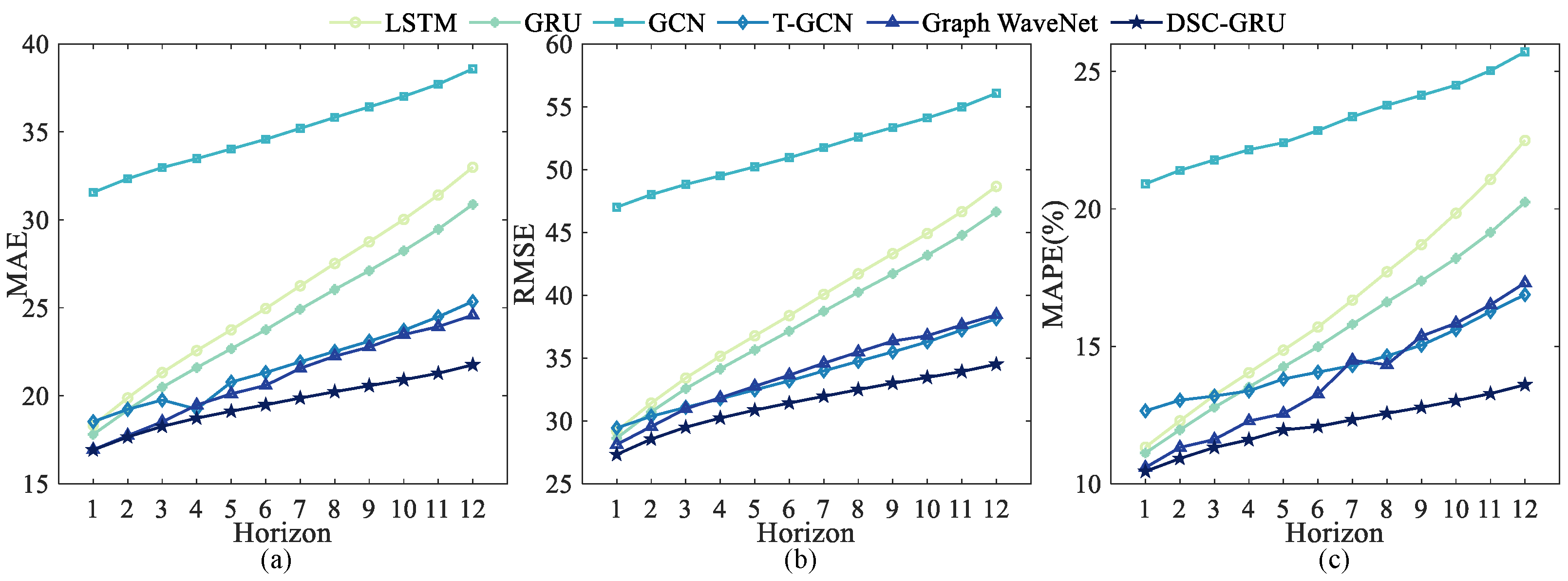
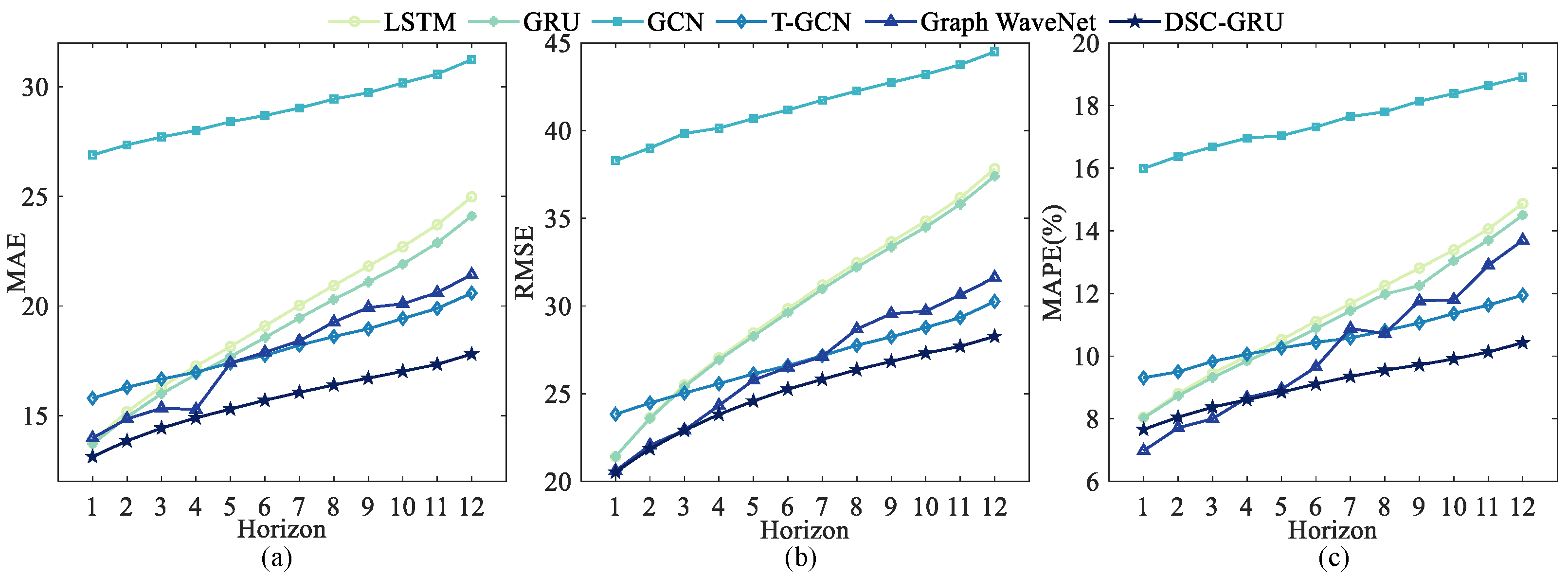
Figure 8 and Figure 9 show the trends of each evaluation metric for different deep learning models based on the PeMS04 and PeMS08 datasets with different horizons. The DSC-GRU model outperforms the the comparison models in all horizons, and the curve rises slowly with the horizon. The experimental results show that our proposed model has better stability.
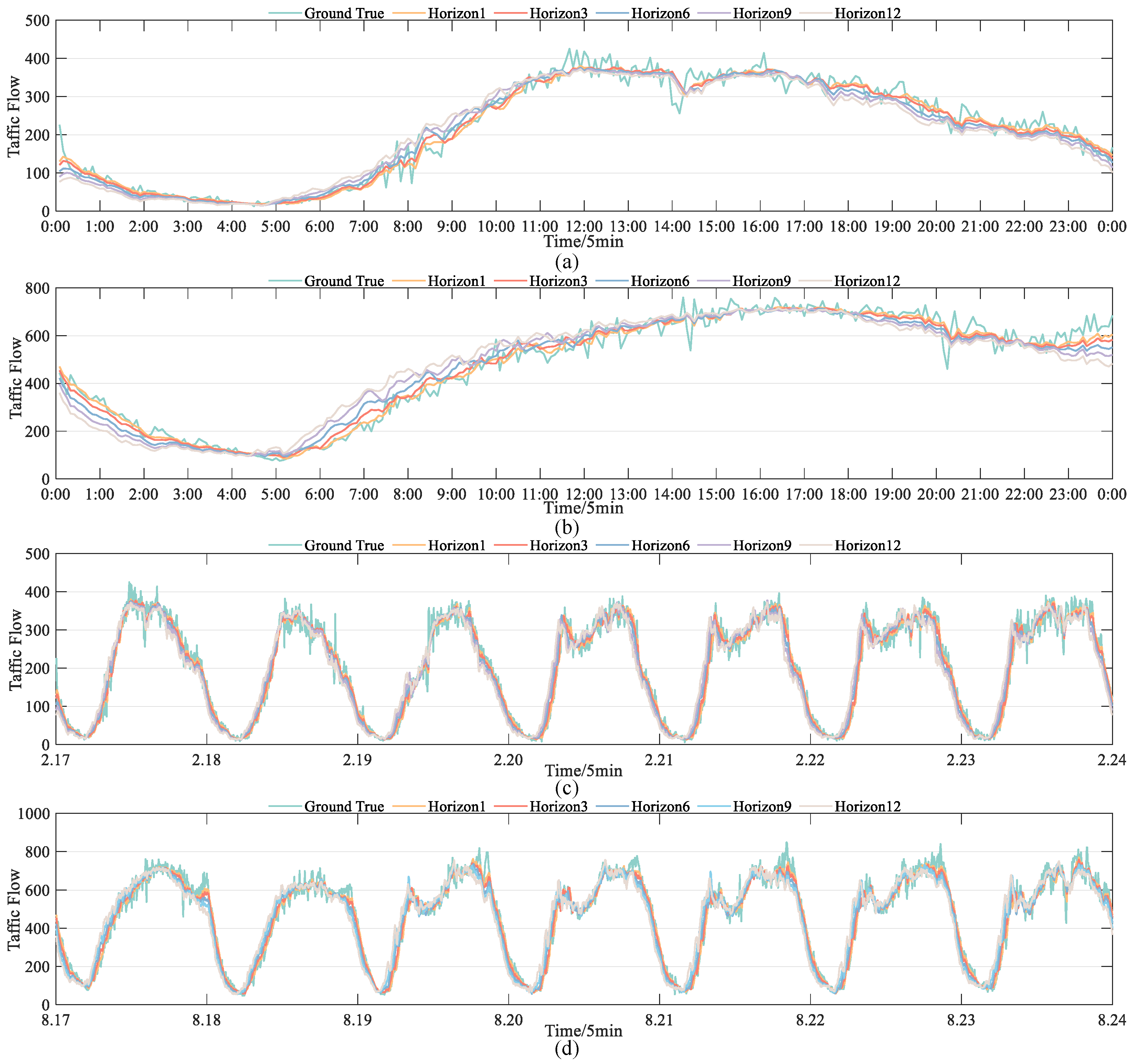
To show the prediction effect of the model more intuitively, the real value and predicted value of the traffic flow data of node 9 for one day and one week in the PeMS04 and PeMS08 datasets are visualized, and the results are shown in Figure 10.
From the visualization results in Figure 10, it can be seen that the model prediction values always follow the real traffic values regardless of all the horizons of the model prediction. This indicates that the DSC-GRU model can correctly consider the spatial and temporal information of the traffic flow data and make predictions.
6.2. Effect of Hyperparameters
This section discusses the role played by three different hyperparameters in the model. The effect of hyperparameters on the prediction performance of the model is tested by altering one of the hyperparameters while ensuring that the other hyperparameters remain constant.
6.2.1. Effect of R2 Threshold Value
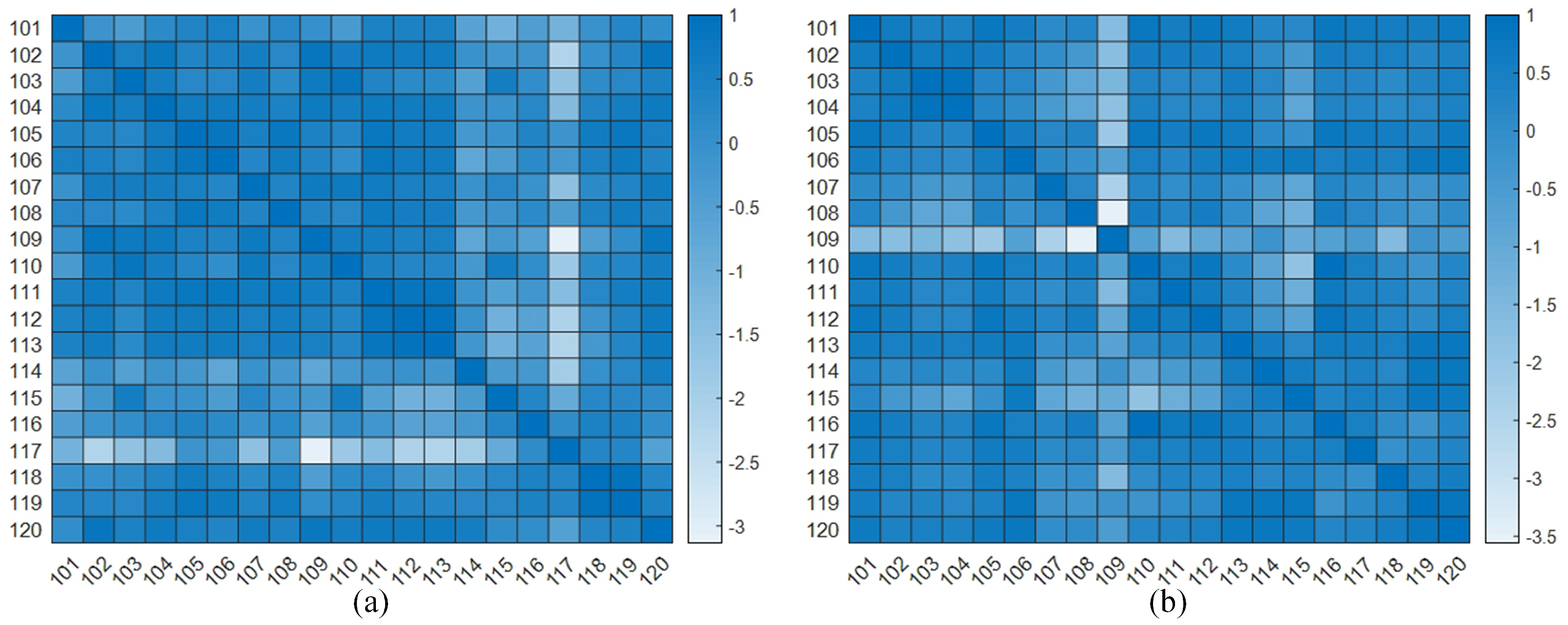
According to Equation (6), the node correlations in the PeMS04 and PeMS08 datasets are calculated. The correlations from node 101 to 120 are visualized and shown in Figure 11.
From the figure above, it can be seen that the magnitude of the correlation between nodes can be effectively quantified by the correlation coefficient. The larger value indicates that the traffic flow state of the corresponding two nodes is more similar. By setting the threshold value, the nodes with similar traffic flow characteristics to the target node are screened out to provide the basis for the model to aggregate the global spatial information of the road network.
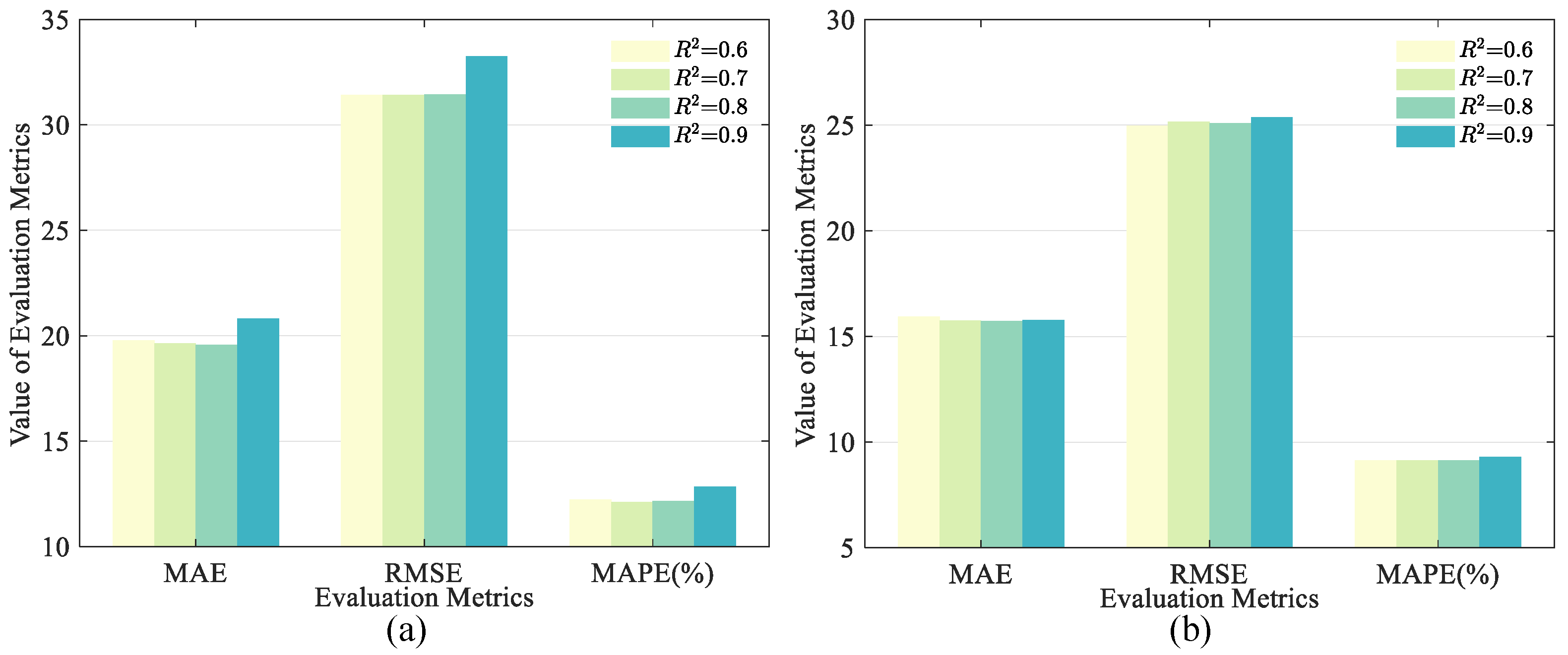
Based on the above analysis, the thresholds affect the information integration of the global space of the road network. They are set to [0.6, 0.7, 0.8, 0.9] according to the case of strong correlation only. By setting different thresholds, the proposed model can control how many nodes are fused to the target node when the global spatial information of the road network is integrated. The larger the threshold, the higher the learning worth of these spatial nodes and the less invalid node information aggregated. The smaller the threshold, the more node information is aggregated, and more spatial information can be obtained. Therefore, it is worth investigating how to set the threshold value so that the model can aggregate the high-quality node information as much as possible while obtaining more spatial information. Therefore, this section tests the model by setting different thresholds to find a balance between high-quality information and more spatial information. and are set to 512 and 128, respectively. The experimental results under different threshold values are shown in Figure 12.
Comparing the experimental results based on the two datasets, it is found that the change trends of the evaluation metrics are not consistent when the threshold value is changed. This is reasonable, because PeMS04 and PeMS08 collect traffic state from different regions. The different spatial characteristics information from the different regions will lead to differences in the model when aggregating spatial information. In addition, the model proposed in this paper has a better ability to fit the traffic flow data when the threshold is set to 0.8.
The experimental results show that in both datasets, setting the threshold too high or too low will lead to a decrease in the predictive ability of the model. This is due to the fact that the larger the threshold is set, the less information is aggregated to the target nodes, which makes the model unable to capture the global spatial structure of the road network well. Conversely, the smaller the threshold is set, the more invalid information is learned by the model, as more information is aggregated to the target node. When the threshold value is set moderately, the model can better balance the amount of aggregated information and the effectiveness of the information.
6.2.2. Effect of Model Structure Parameters
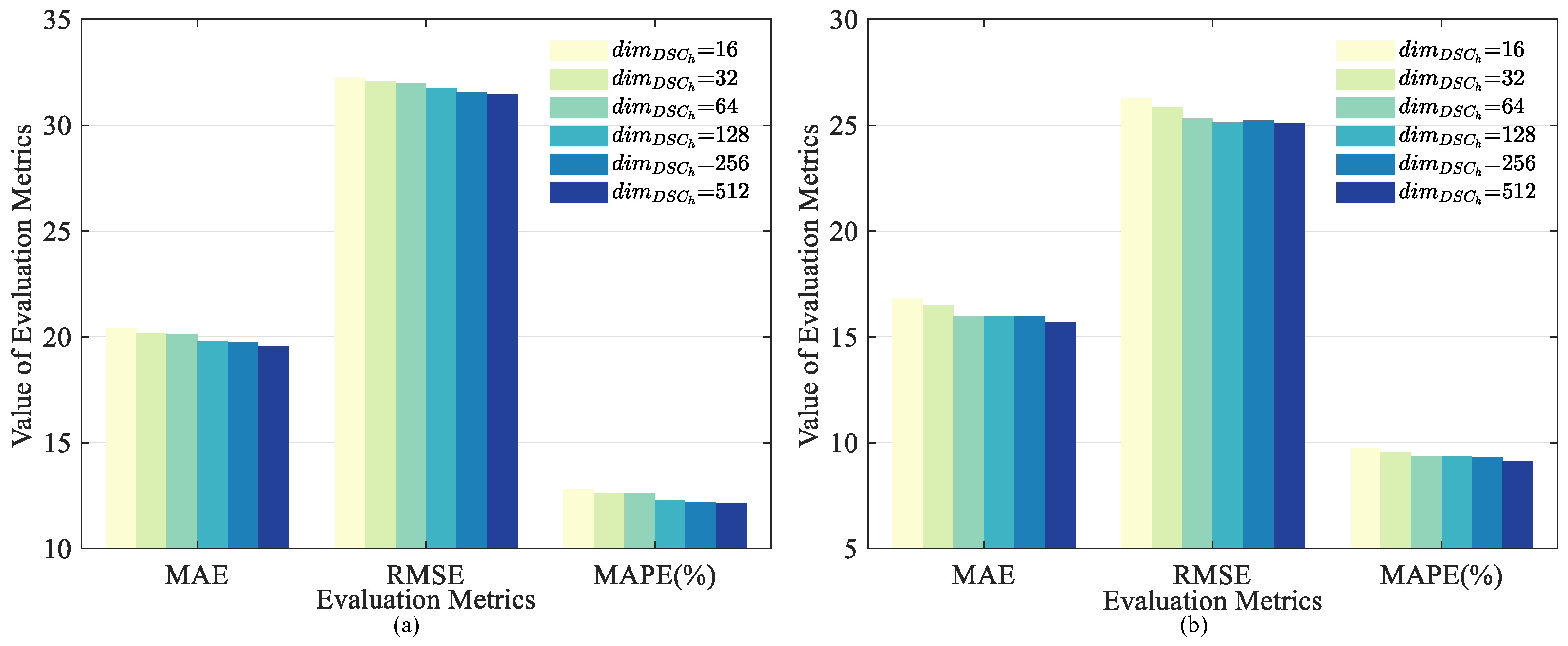
The number of neurons in the hidden layer will affect the fitting ability of the model. Too few neurons may lead to the insufficient ability of the model to extract features from traffic flow data. Too many neurons may increase the burden of the model and make the model training time costlier [47].
Considering that the GCN network in the DSC processes the entire input data, increasing the number of hidden layer neurons has little impact on the training time of the model; so, is set to [16, 32, 64, 128, 256, 512]. In addition, the threshold is set to 0.8 and is set to 128. The experimental results are shown in Figure 13.
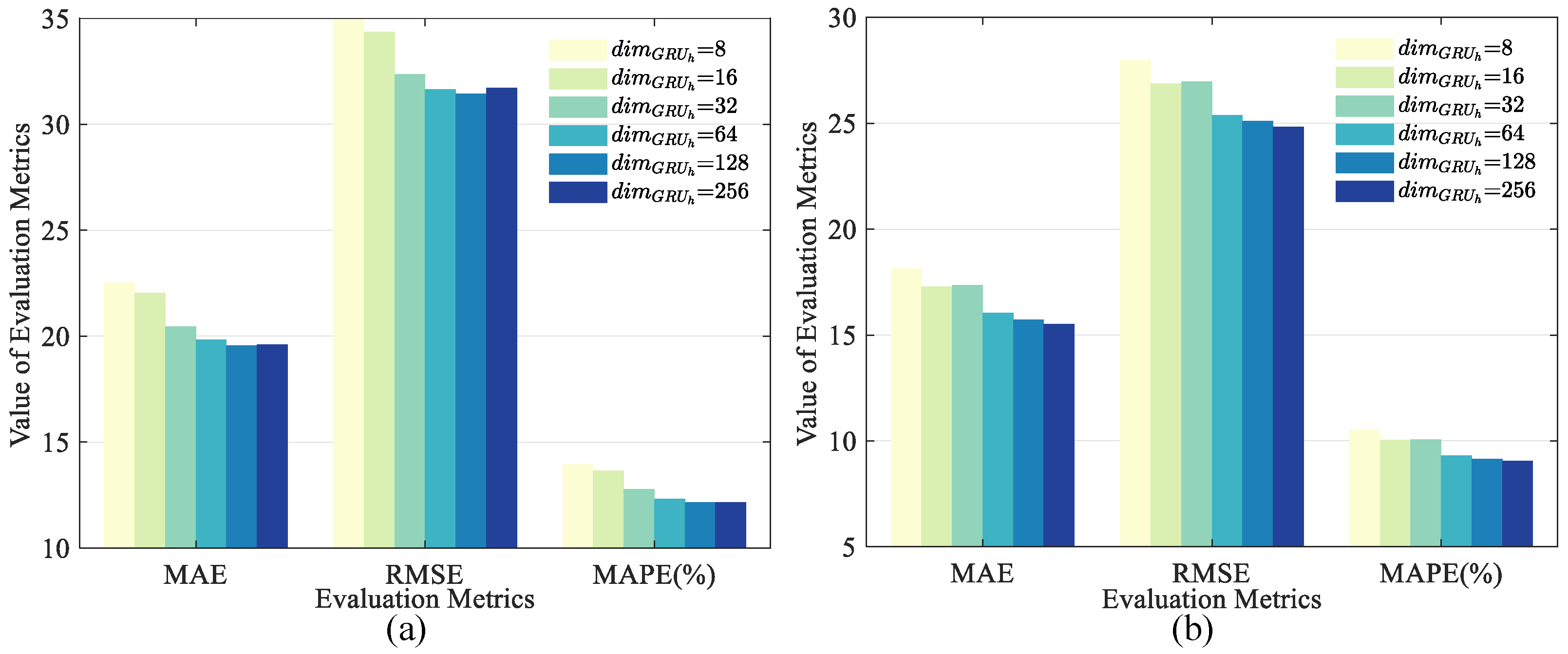
Similarly, since the GRU must process the input at each time step, increasing the number of hidden layer neurons will lead to a significant increase in model training time; so, is set to [8, 16, 32, 64, 128, 256]. In addition, the threshold is set to 0.8 and is set to 512. The experimental results are shown in Figure 14.
According to the experimental results, we can draw the following conclusions. First of all, the DSC-GRU model is insensitive to the , but it does decrease slowly. The GCN in the DSC has the properties of local correlation and shared weight. These properties allow the DSC to capture structural information between nodes and have some robustness to changes in hidden layer neurons while maintaining the structure unchanged. Simultaneously, as the increases, the prediction accuracy of the model initially improves rapidly. The GRU introduces gated mechanisms to control the flow of information, and the parameters of these gated units are learned through the network. When there is a change in the , it affects the input and output of the gated units, which in turn affects the flow and storage of information. Therefore, the GRU model is sensitive to the . After the reaches a certain number, the improvement of model accuracy by increasing the number of neurons becomes weak. This is because too large a may lead to overfitting, which limits performance gains. The cost of model training increases significantly as the number of neurons grows. The other parameters remain unchanged. When the is set to 512, the training time to an epoch is already twice as long as when the number of neurons is 16. Similarly, when the is set to 128, the training time to an epoch is already three times as long as that of 8 neurons. It is undeniable that increasing the number of neurons can improve the accuracy of the model. Still, it is meaningless to blindly increase the number of neurons wihtout considering the significant increase in training cost.
6.3. Ablation Experiments
The DSC-GRU model consists of two components based on the gated mechanism: the dual spatial graph convolution and the temporal dependence recurrent neural network. To explore the performance of each component, the prediction performance is compared between the DSC-GRU model and its two components.
The ablation experiments are set up as follows. (1) DSC: this model ignores the time dependence in the traffic data and only considers the entire spatial topological structure of the road network. (2) GRU: the traditional GRU model considers the long-term temporal dependence of the traffic data but ignores the spatial topological structure of the road network. The threshold is set to 0.8, and the and are set to 512 and 128, respectively. The experimental results are shown in Table 3.
The experiment results show that DSC has the worst prediction accuracy, because traffic flow data are essentially a kind of time series data. The potential time dependence in the historical traffic flow data will affect the prediction results. The DSC model only considers the spatial dependence but ignores the time dependence, and the poor prediction accuracy is reasonable. The GRU model considers the feature that traffic flow data are highly correlated in the temporal dimension and therefore has better prediction performance compared with DSC. In addition, since the DSC-GRU considers the spatiotemporal dependence of traffic flow data, the accuracy of the model is better than any of the components. In the first place, it proves the significance of considering the spatiotemporal dependence of traffic data to improve traffic flow prediction accuracy. In the second place, it demonstrates the effectiveness of the DSC-GRU model for solving the traffic flow prediction task.
7. Conclusions
In this paper, we propose a deep learning model, termed DSC-GRU, which can simultaneously consider the spatiotemporal characteristics of traffic flow data to deal with traffic flow prediction task. On the one hand, the DSC unit is used to capture the topological structure of the road network space and model the spatial dependence of traffic data. Unlike the traditional graph convolutional networks that only consider the characteristics of neighbor nodes, the DSC also considers the global characteristics of nodes in the whole road network space based on the correlation matrix. The gated mechanism is introduced to control the relative importance relationship between the adjacent information and the global information. The impact of the spatial dependence of the traffic road network are fully considered. On the other hand, the GRU is used to capture the characteristics of dynamic changes in traffic flow and to model the time dependence of traffic data. The DSC unit is embedded in the GRU network to add spatial information to each state in the GRU network. Based on two real-world datasets, parametric experiments and ablation experiments are conducted to select the optimal structure and parameters. Comparison experiments show that the DSC-GRU model has better prediction performance at different horizons and outperforms each of the comparison models. In conclusion, the DSC-GRU can be extended to other prediction tasks with spatiotemporal characteristics.
The DSC-GRU model still has some shortcomings. The influence of external factors is not considered in the model. The effects of weather, traffic accidents, and surrounding buildings should be considered to make the predicted traffic flow data more realistic. In subsequent work, the dataset containing the above information needs to be selected for further validation of our proposed model.
Author Contributions
Conceptualization, Qingyong Zhang and Lingfeng Zhou; data curation, Bingrong Xu; formal analysis, Yixin Su; funding acquisition, Yixin Su; investigation, Yixin Su; methodology, Qingyong Zhang; project administration, Yixin Su; resources, Bingrong Xu; software, Huiwen Xia; supervision, Qingyong Zhang; validation, Qingyong Zhang and Lingfeng Zhou; visualization, Qingyong Zhang and Huiwen Xia; writing—original draft, Lingfeng Zhou; writing—review and editing, Lingfeng Zhou. All authors have read and agreed to the published version of the manuscript.
Funding
This research was funded by the National Natural Science Foundation of China under Grant (62206204) and the Natural Science Foundation of Hubei Province grant number [2019CFB571].
Institutional Review Board Statement
Not applicable.
Informed Consent Statement
Not applicable.
Data Availability Statement
A publicly available dataset was analyzed in this study. It can be found here: https://github.com/wanhuaiyu/ASTGCN/tree/master/data, accessed on 1 June 2023.
Acknowledgments
The authors would like to thank the National Natural Science Foundation of China under Grant (62206204) and the Natural Science Foundation of Hubei Province grant number [2019CFB571] for supporting this research.
Conflicts of Interest
The authors declare no conflict of interest. The funder had no role in the design of the study, in the collection, analysis, or interpretation; in the writing of the manuscript; or in the decision to publish the results.
Appendix A. The Pseudocode of DSC_GRU Training
| Algorithm A1 The training of DSC_GRU |
| Input: Traffic flow data at t moment . Initial hidden state . Traffic flow true value Y. Traffic road network . |
| Output: Predicted value . Training epochs . |
| Initialize: The length of historical data used for prediction h. Hidden layer state . Process the adjacent graph . Process the global graph . Loss function . |
|
References
- Liu, Y.; James, J.; Kang, J.; Niyato, D.; Zhang, S. Privacy-preserving traffic flow prediction: A federated learning approach. IEEE Internet Things J. 2020, 7, 7751–7763. [Google Scholar] [CrossRef]
- Lin, X.; Sun, X.; Ho, P.H.; Shen, X. GSIS: A secure and privacy-preserving protocol for vehicular communications. IEEE Trans. Veh. Technol. 2007, 56, 3442–3456. [Google Scholar]
- Yu, B.; Yin, H.; Zhu, Z. Spatio-temporal graph convolutional networks: A deep learning framework for traffic forecasting. arXiv 2017, arXiv:1709.04875. [Google Scholar]
- Kumar, S.V.; Vanajakshi, L. Short-term traffic flow prediction using seasonal ARIMA model with limited input data. Eur. Transp. Res. Rev. 2015, 7, 21. [Google Scholar] [CrossRef]
- Emami, A.; Sarvi, M.; Bagloee, S.A. Short-term traffic flow prediction based on faded memory Kalman Filter fusing data from connected vehicles and Bluetooth sensors. Simul. Model. Pract. Theory 2020, 102, 102025. [Google Scholar] [CrossRef]
- Wang, H.; Liu, L.; Dong, S.; Qian, Z.; Wei, H. A novel work zone short-term vehicle-type specific traffic speed prediction model through the hybrid EMD–ARIMA framework. Transp. B-Transp. Dyn. 2016, 4, 159–186. [Google Scholar] [CrossRef]
- Zhang, X.; He, G.; Lu, H. Short-term traffic flow forecasting based on K-nearest neighbors non-parametric regression. J. Card. Surg. 2009, 24, 178–183. [Google Scholar]
- Petrlik, J.; Fucik, O.; Sekanina, L. Multiobjective selection of input sensors for svr applied to road traffic prediction. In Proceedings of the International Conference on Parallel Problem Solving from Nature, Ljubljana, Slovenia, 13–17 September 2014; pp. 802–811. [Google Scholar]
- Westgate, B.S.; Woodard, D.B.; Matteson, D.S.; Henderson, S.G. Travel time estimation for ambulances using Bayesian data augmentation. Ann. Appl. Stat. 2013, 7, 1139–1161. [Google Scholar] [CrossRef]
- Chen, X.; Wu, S.; Shi, C.; Huang, Y.; Yang, Y.; Ke, R.; Zhao, J. Sensing data supported traffic flow prediction via denoising schemes and ANN: A comparison. IEEE Sens. J. 2020, 20, 14317–14328. [Google Scholar] [CrossRef]
- Cai, Q.; Abdel-Aty, M.; Sun, Y.; Lee, J.; Yuan, J. Applying a deep learning approach for transportation safety planning by using high-resolution transportation and land use data. Transp. Res. Part A-Policy Pract. 2019, 127, 71–85. [Google Scholar] [CrossRef]
- Van Lint, J.; Hoogendoorn, S.P.; van Zuylen, H.J. Freeway travel time prediction with state-space neural networks: Modeling state-space dynamics with recurrent neural networks. Transp. Res. Rec. 2002, 1811, 30–39. [Google Scholar] [CrossRef]
- Hochreiter, S.; Schmidhuber, J. Long short-term memory. Neural Comput. 1997, 9, 1735–1780. [Google Scholar] [CrossRef] [PubMed]
- Parizad, A.; Hatziadoniu, C. Deep Learning Algorithms and Parallel Distributed Computing Techniques for High-Resolution Load Forecasting Applying Hyperparameter Optimization. IEEE Syst. J. 2022, 16, 3758–3769. [Google Scholar] [CrossRef]
- Zhang, Q.; Li, C.; Su, F.; Li, Y. Spatio-Temporal Residual Graph Attention Network for Traffic Flow Forecasting. IEEE Internet Things J. 2023, 10, 11518–11532. [Google Scholar] [CrossRef]
- Liao, Z.; Huang, H.; Zhao, Y.; Liu, Y.; Zhang, G. Analysis and Forecast of Traffic Flow between Urban Functional Areas Based on Ride-Hailing Trajectories. ISPRS Int. J. Geo-Inf. 2023, 12, 144. [Google Scholar] [CrossRef]
- Méndez, M.; Merayo, M.G.; Núñez, M. Long-term traffic flow forecasting using a hybrid CNN-BiLSTM model. Eng. Appl. Artif. Intell. 2023, 121, 106041. [Google Scholar] [CrossRef]
- Peng, H.; Wang, H.; Du, B.; Bhuiyan, M.Z.A.; Ma, H.; Liu, J.; Wang, L.; Yang, Z.; Du, L.; Wang, S.; et al. Spatial temporal incidence dynamic graph neural networks for traffic flow forecasting. Inf. Sci. 2020, 521, 277–290. [Google Scholar] [CrossRef]
- Yin, X.; Wu, G.; Wei, J.; Shen, Y.; Qi, H.; Yin, B. Deep learning on traffic prediction: Methods, analysis, and future directions. IEEE Trans. Intell. Transp. Syst. 2021, 23, 4927–4943. [Google Scholar] [CrossRef]
- Lin, G.; Lin, A.; Gu, D. Using support vector regression and K-nearest neighbors for short-term traffic flow prediction based on maximal information coefficient. Inf. Sci. 2022, 608, 517–531. [Google Scholar] [CrossRef]
- Zhang, Q.; Yin, C.; Chen, Y.; Su, F. IGCRRN: Improved Graph Convolution Res-Recurrent Network for spatio-temporal dependence capturing and traffic flow prediction. Eng. Appl. Artif. Intell. 2022, 114, 105179. [Google Scholar] [CrossRef]
- Nadarajan, J.; Sivanraj, R. Attention-Based Multiscale Spatiotemporal Network for Traffic Forecast with Fusion of External Factors. ISPRS Int. J. Geo Inf. 2022, 11, 619. [Google Scholar] [CrossRef]
- Yue, W.; Zhou, D.; Wang, S.; Duan, P. Engineering Traffic Prediction with Online Data Imputation: A Graph-Theoretic Perspective. IEEE Syst. J. 2023, 17, 4485–4496. [Google Scholar] [CrossRef]
- Wang, T.; Zhang, B.; Wei, W.; Damaševičius, R.; Scherer, R. Traffic flow prediction based on BP neural network. In Proceedings of the International Conference on AIID, Guangzhou, China, 28–30 May 2021; pp. 15–19. [Google Scholar]
- Huang, W.; Song, G.; Hong, H.; Xie, K. Deep architecture for traffic flow prediction: Deep belief networks with multitask learning. IEEE Trans. Intell. Transp. Syst. 2014, 15, 2191–2201. [Google Scholar] [CrossRef]
- Lv, Y.; Duan, Y.; Kang, W.; Li, Z.; Wang, F.Y. Traffic flow prediction with big data: A deep learning approach. IEEE Trans. Intell. Transp. Syst. 2014, 16, 865–873. [Google Scholar] [CrossRef]
- Ma, X.; Tao, Z.; Wang, Y.; Yu, H.; Wang, Y. Long short-term memory neural network for traffic speed prediction using remote microwave sensor data. Transp. Res. Part C-Emerg. Technol. 2015, 54, 187–197. [Google Scholar] [CrossRef]
- Sun, P.; Boukerche, A.; Tao, Y. SSGRU: A novel hybrid stacked GRU-based traffic volume prediction approach in a road network. Comput. Commun. 2020, 160, 502–511. [Google Scholar] [CrossRef]
- Cho, K.; Van Merriënboer, B.; Gulcehre, C.; Bahdanau, D.; Bougares, F.; Schwenk, H.; Bengio, Y. Learning phrase representations using RNN encoder-decoder for statistical machine translation. arXiv 2014, arXiv:1406.1078. [Google Scholar]
- Sutskever, I.; Vinyals, O.; Le, Q.V. Sequence to sequence learning with neural networks. Adv. Neural Inf. Process. Syst. 2014, 27. [Google Scholar]
- Zheng, G.; Chai, W.K.; Katos, V.; Walton, M. A joint temporal-spatial ensemble model for short-term traffic prediction. Neural Comput. 2021, 457, 26–39. [Google Scholar] [CrossRef]
- Ma, X.; Dai, Z.; He, Z.; Ma, J.; Wang, Y.; Wang, Y. Learning traffic as images: A deep convolutional neural network for large-scale transportation network speed prediction. Sensors 2017, 17, 818. [Google Scholar] [CrossRef]
- Shi, X.; Chen, Z.; Wang, H.; Yeung, D.Y.; Wong, W.K.; Woo, W.c. Convolutional LSTM network: A machine learning approach for precipitation nowcasting. Adv. Neural Inf. Process. Syst. 2015, 28. [Google Scholar] [CrossRef]
- Zhao, L.; Song, Y.; Zhang, C.; Liu, Y.; Wang, P.; Lin, T.; Deng, M.; Li, H. T-gcn: A temporal graph convolutional network for traffic prediction. IEEE Trans. Intell. Transp. Syst. 2019, 21, 3848–3858. [Google Scholar] [CrossRef]
- Guo, S.; Lin, Y.; Feng, N.; Song, C.; Wan, H. Attention based spatial-temporal graph convolutional networks for traffic flow forecasting. In Proceedings of the AAAI Conference Artificial Intelligence, Honolulu, HI, USA, 27 January–1 February 2019; Volume 33, pp. 922–929. [Google Scholar]
- Huang, Y.; Weng, Y.; Yu, S.; Chen, X. Diffusion convolutional recurrent neural network with rank influence learning for traffic forecasting. In Proceedings of the 2019 IEEE 3rd Information Technology, Networking, Electronic and Automation Control Conference (ITNEC), Chengdu, China, 15–17 March 2019; pp. 678–685. [Google Scholar]
- Bao, Y.; Huang, J.; Shen, Q.; Cao, Y.; Ding, W.; Shi, Z.; Shi, Q. Spatial–Temporal Complex Graph Convolution Network for Traffic Flow Prediction. Eng. Appl. Artif. Intell. 2023, 121, 106044. [Google Scholar] [CrossRef]
- Wu, Z.; Pan, S.; Long, G.; Jiang, J.; Zhang, C. Graph wavenet for deep spatial-temporal graph modeling. arXiv 2019, arXiv:1906.00121. [Google Scholar]
- Song, C.; Lin, Y.; Guo, S.; Wan, H. Spatial-temporal synchronous graph convolutional networks: A new framework for spatial-temporal network data forecasting. In Proceedings of the AAAI Conference on Artificial Intelligence, Hilton, NY, USA, 7–12 February 2020; Volume 34, pp. 914–921. [Google Scholar]
- Hao, S.; Lee, D.H.; Zhao, D. Sequence to sequence learning with attention mechanism for short-term passenger flow prediction in large-scale metro system. Transp. Res. Part C-Emerg. Technol. 2019, 107, 287–300. [Google Scholar] [CrossRef]
- Li, Z.; Han, Y.; Xu, Z.; Zhang, Z.; Sun, Z.; Chen, G. PMGCN: Progressive Multi-Graph Convolutional Network for Traffic Forecasting. ISPRS Int. J. Geo-Inf. 2023, 12, 241. [Google Scholar] [CrossRef]
- Defferrard, M.; Bresson, X.; Vandergheynst, P. Convolutional neural networks on graphs with fast localized spectral filtering. Adv. Neural Inf. Process. Syst. 2016, 29. [Google Scholar] [CrossRef]
- Engelmann, F.; Bokeloh, M.; Fathi, A.; Leibe, B.; Nießner, M. 3d-mpa: Multi-proposal aggregation for 3d semantic instance segmentation. In Proceedings of the IEEE Conference Computer Vision and Pattern Recognition, Seattle, WA, USA, 14–19 June 2020; pp. 9031–9040. [Google Scholar]
- Gligorijević, V.; Renfrew, P.D.; Kosciolek, T.; Leman, J.K.; Berenberg, D.; Vatanen, T.; Chandler, C.; Taylor, B.C.; Fisk, I.M.; Vlamakis, H.; et al. Structure-based protein function prediction using graph convolutional networks. Nat. Commun. 2021, 12, 3168. [Google Scholar] [CrossRef] [PubMed]
- Adem, K. Diagnosis of breast cancer with Stacked autoencoder and Subspace kNN. Phys. A 2020, 551, 124591. [Google Scholar] [CrossRef]
- Chen, X.; Wang, X.; Yi, B.; He, Q.; Huang, M. Deep Learning-Based Traffic Prediction for Energy Efficiency Optimization in Software-Defined Networking. IEEE Syst. J. 2021, 15, 5583–5594. [Google Scholar] [CrossRef]
- Guo, S.; Lin, Y.; Wan, H.; Li, X.; Cong, G. Learning dynamics and heterogeneity of spatial-temporal graph data for traffic forecasting. IEEE Trans. Knowl. Data Eng. 2021, 34, 5415–5428. [Google Scholar] [CrossRef]
Figure 1.
Effect of the topological structure. Similar trends exist between nodes.

Figure 2.
Periodicity of traffic flow data: (a) Daily periodicity. (b) Weekly periodicity. ① traffic flow data of a workday. ② traffic flow data of a weekday. ③ traffic flow data of a holiday. ④ traffic flow data of one week.
Figure 2.
Periodicity of traffic flow data: (a) Daily periodicity. (b) Weekly periodicity. ① traffic flow data of a workday. ② traffic flow data of a weekday. ③ traffic flow data of a holiday. ④ traffic flow data of one week.

Figure 3.
Framework of the DSC-GRU model.

Figure 4.
Node distribution: (a) Adjacent space. (b) Global space.

Figure 5.
Integration process: (a) Adjacent space. (b) Global space.

Figure 6.
The overall structure of the DSC unit.

Figure 7.
The overall prediction process of the DSC-GRU model.

Figure 8.
Evaluation metrics at different horizons of the model on PeMS04: (a) MAE. (b) RMSE. (c) MAPE.
Figure 8.
Evaluation metrics at different horizons of the model on PeMS04: (a) MAE. (b) RMSE. (c) MAPE.

Figure 9.
Evaluation metrics at different horizons of the model on PeMS08: (a) MAE. (b) RMSE. (c) MAPE.
Figure 9.
Evaluation metrics at different horizons of the model on PeMS08: (a) MAE. (b) RMSE. (c) MAPE.

Figure 10.
Visualization of prediction results: (a) One-day traffic flow at node 9 on PeMS04. (b) One-day traffic flow at node 9 on PeMS08. (c) One-week traffic flow at node 9 on PeMS04. (d) One-week traffic flow at node 9 on PeMS08.
Figure 10.
Visualization of prediction results: (a) One-day traffic flow at node 9 on PeMS04. (b) One-day traffic flow at node 9 on PeMS08. (c) One-week traffic flow at node 9 on PeMS04. (d) One-week traffic flow at node 9 on PeMS08.

Figure 11.
Partial node correlation heat map: (a) Heatmap for PeMS04. (b) Heatmap for PeMS08.

Figure 12.
Evaluation metrics under different threshold values: (a) PeMS04. (b) PeMS08.

Figure 13.
Evaluation metrics under different numbers of DSC hidden layer neurons: (a) PeMS04. (b) PeMS08.
Figure 13.
Evaluation metrics under different numbers of DSC hidden layer neurons: (a) PeMS04. (b) PeMS08.

Figure 14.
Evaluation metrics under different numbers of GRU hidden layer neurons: (a) PeMS04. (b) PeMS08.
Figure 14.
Evaluation metrics under different numbers of GRU hidden layer neurons: (a) PeMS04. (b) PeMS08.


Table 1.
The relationship between the correlation coefficient and correlation strength.
| The Value Range of | Correlation Strength |
|---|---|
| None | |
| Weak | |
| Moderate | |
| Strong | |
| Extreme |
Table 2.
The performance comparison of different models.
| Models | PeMS04 | PeMS08 | |||||||
|---|---|---|---|---|---|---|---|---|---|
| MAE | RMSE | MAPE | MAE | RMSE | MAPE | ||||
| HA | 38.09 | 54.51 | 28.38% | 0.880 | 32.14 | 46.06 | 20.36% | 0.900 | |
| ARIMA | 35.19 | 50.05 | 24.18% | 0.889 | 29.12 | 41.95 | 18.32% | 0.912 | |
| LSTM | 25.64 | 39.13 | 16.49% | 0.937 | 19.50 | 30.16 | 11.45% | 0.956 | |
| GRU | 24.35 | 37.84 | 15.50% | 0.942 | 18.97 | 29.96 | 11.19% | 0.957 | |
| GCN | 34.98 | 51.45 | 23.17% | 0.894 | 28.97 | 41.55 | 17.49% | 0.923 | |
| T-GCN | 21.74 | 34.28 | 14.02% | 0.951 | 18.05 | 26.93 | 10.57% | 0.964 | |
| Graph WaveNet | 20.96 | 33.94 | 13.76% | 0.956 | 17.87 | 26.63 | 10.12% | 0.967 | |
| DSC-GRU | 19.56 | 31.44 | 12.15% | 0.960 | 15.72 | 25.10 | 9.14% | 0.970 | |
Table 3.
The result of ablation experiments.
| Models | PeMS04 | PeMS08 | |||||||
|---|---|---|---|---|---|---|---|---|---|
| MAE | RMSE | MAPE | MAE | RMSE | MAPE | ||||
| DSC | 27.13 | 40.58 | 17.95% | 0.934 | 22.02 | 32.82 | 13.07% | 0.949 | |
| GRU | 24.35 | 37.84 | 15.50% | 0.942 | 18.97 | 29.96 | 11.19% | 0.957 | |
| DSC-GRU | 19.56 | 31.44 | 12.15% | 0.960 | 15.72 | 25.10 | 9.14% | 0.970 | |
Disclaimer/Publisher’s Note: The statements, opinions and data contained in all publications are solely those of the individual author(s) and contributor(s) and not of MDPI and/or the editor(s). MDPI and/or the editor(s) disclaim responsibility for any injury to people or property resulting from any ideas, methods, instructions or products referred to in the content. |
© 2023 by the authors. Licensee MDPI, Basel, Switzerland. This article is an open access article distributed under the terms and conditions of the Creative Commons Attribution (CC BY) license (https://creativecommons.org/licenses/by/4.0/).
Share and Cite
MDPI and ACS Style
Zhang, Q.; Zhou, L.; Su, Y.; Xia, H.; Xu, B. Gated Recurrent Unit Embedded with Dual Spatial Convolution for Long-Term Traffic Flow Prediction. ISPRS Int. J. Geo-Inf. 2023, 12, 366. https://doi.org/10.3390/ijgi12090366
AMA Style
Zhang Q, Zhou L, Su Y, Xia H, Xu B. Gated Recurrent Unit Embedded with Dual Spatial Convolution for Long-Term Traffic Flow Prediction. ISPRS International Journal of Geo-Information. 2023; 12(9):366. https://doi.org/10.3390/ijgi12090366
Chicago/Turabian StyleZhang, Qingyong, Lingfeng Zhou, Yixin Su, Huiwen Xia, and Bingrong Xu. 2023. "Gated Recurrent Unit Embedded with Dual Spatial Convolution for Long-Term Traffic Flow Prediction" ISPRS International Journal of Geo-Information 12, no. 9: 366. https://doi.org/10.3390/ijgi12090366
Note that from the first issue of 2016, this journal uses article numbers instead of page numbers. See further details here.