

Modelling Global Deforestation Using Spherical Geographic Automata Approach

Spatial Analysis and Modeling Laboratory, Department of Geography, Simon Fraser University, Burnaby, BC V5A 1S6, Canada
*
Author to whom correspondence should be addressed.
ISPRS Int. J. Geo-Inf. 2023, 12(8), 306; https://doi.org/10.3390/ijgi12080306
Submission received: 16 June 2023
/
Revised: 12 July 2023
/
Accepted: 26 July 2023
/
Published: 28 July 2023
Abstract
:Deforestation as a land-cover change process is linked to several environmental problems including desertification, biodiversity loss, and ultimately climate change. Understanding the land-cover change process and its relation to human–environment interactions is important for supporting spatial decisions and policy making at the global level. However, current geosimulation model applications mainly focus on characterizing urbanization and agriculture expansion. Existing modelling approaches are also unsuitable for simulating land-cover change processes covering large spatial extents. Thus, the objective of this research is to develop and implement a spherical geographic automata model to simulate deforestation at the global level under different scenarios designed to represent diverse future conditions. Simulation results from the deforestation model indicate the global forest size would decrease by 10.5% under the “business-as-usual” scenario through 2100. The global forest extent would also decline by 15.3% under the accelerated deforestation scenario and 3.7% under the sustainable deforestation scenario by the end of the 21st century. The obtained simulation outputs also revealed the rate of deforestation in protected areas to be considerably lower than the overall forest-cover change rate under all scenarios. The proposed model can be utilized by stakeholders to examine forest conservation programs and support sustainable policy making and implementation.
1. Introduction
Deforestation is a land-cover change (LCC) process caused by natural and anthropogenic factors further entailing environmental degradation with several negative consequences both at the regional and global scales [1,2]. Rates of deforestation especially in developing countries, triggered by factors such as agricultural expansion, timber production, forest fire, mining, and urbanization have been increasing over the last century [3,4,5]. These trends of decreasing forest cover and deteriorating conditions have resulted in deforestation becoming a major global environmental issue considering the several critically important ecosystem services and functions forests provide [6,7]. Forests are important areas for biodiversity, with approximately 80% of the world’s terrestrial biodiversity found in forest regions [8]. Further, forests represent the largest terrestrial sink of carbon dioxide (CO2) and are globally responsible for significant carbon stocks [9,10]. These highlight the important roles forests play in the Earth’s biochemical and ecological systems.
Geosimulation modelling has become an important tool for representing land-cover change (LCC) processes and assisting in understanding the interaction between anthropogenic activities and the impact of deforestation on other environmental systems, permitting spatial analyses of the underlying causes of this dynamic process [11]. Further, the simulation of possible LCC scenarios provides a useful mechanism to inform environmental and forest management policies and decision making for providing valuable insights for developing appropriate measures to alleviate the negative impacts of deforestation [12]. Specifically, data on forest cover and future trajectories provide significant information for estimating carbon stocks, ecosystem service evaluation, and forestry conservation [13,14]. Assessing the performance and effectiveness of environmental policies such as the Reduction in Emissions from Deforestation and Forest Degradation (REDD+) policies requires detailed spatial data on forest-cover change and future scenarios [15].
Forests can be considered as complex biophysical spatial systems with many components, and some considerably depend on human interactions at the local level to give rise to global patterns of deforestation processes over time [16]. Thus, geosimulation modelling approaches are seen as suitable for representing forest change processes. Accordingly, several geosimulation models have been implemented to represent the dynamics of forest changes as a complex spatial process including approaches based on cellular automata (CA) [17,18], and some were enhanced with techniques such as Markov chain [19,20], logistic regression [21,22], multi-criteria evaluation (MCE) [23,24], machine learning [25], and deep learning [26]. Several studies have also been incorporating human interactions to represent deforestation processes using agent-based geosimulation models (ABMs) [27,28]. However, these modelling approaches are all developed mainly to operate on small spatial extents and implemented to simulate forest-cover change dynamics at the local and regional levels.
The use of existing geosimulation models at larger spatial scales presents challenges that are peculiar to spatial modelling at the global level. Primarily, these models do not consider the curvature of the Earth’s surface when modelling at larger extents, which can lead to errors in spatial and statistical analyses due to spatial distortions caused by planar map projections [29]. The limitations of using planar spatial models for analyses and simulations at the global level have been documented in the scientific literature [30,31,32], with spherical models proposed as a possible solution. While spatially explicit land-cover change models have become prevalent over the last decade, geosimulation models for deforestation are still scarce, with existing global applications typically focusing on simulating urbanization [33,34] and agricultural expansion [35]. In order to improve simulation results, CA models are often integrated with other techniques such as spatial multi-criteria evaluation (MCE) to identify suitable or susceptible locations for the potential occurrence of the geographic phenomena and then guide transition rules. The MCE technique provides a comprehensive approach that combines several often-conflicting criteria based on suitability functions, weights, and their overall aggregation [36]. The approach has been implemented in several applications, including land-cover change [37,38], deforestation [23], and urban growth [39], although all these studies address small spatial extents. Therefore, the main objective of this research study is to develop and implement a spherical geographic automata (SGA) modelling approach by integrating MCE and cellular automata to simulate the process of deforestation at the global level and considering the curved surface of the Earth.
2. Materials and Methods
2.1. Spherical Deforestation Model Overview
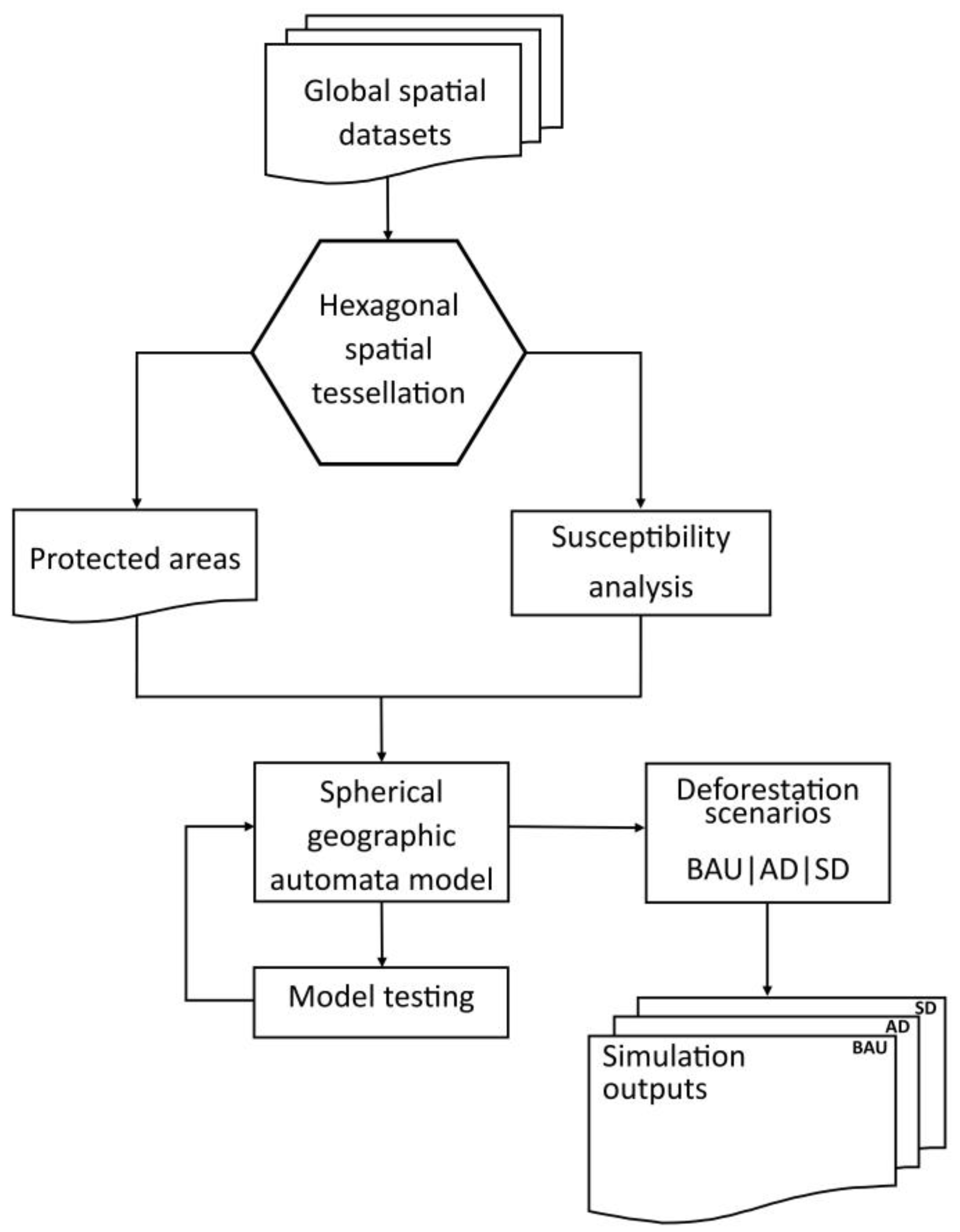
The methodology extends the theoretical concepts of the spherical geographic automata (SGA) approach [40] and integrates susceptibility analysis for global deforestation modelling. The methodological flow chart of the modelling approach is presented in Figure 1. The spherical component of the model is operationalized with the use of a discrete global grid system (DGGS) [41] and hexagonal spatial tessellations as a base unit that allows for geospatial data representation at the global level and with consideration of the curvature of the Earth’s surface. The MCE technique is used to identify susceptible locations for forest-cover loss using several criteria as possible drivers of deforestation. Three scenarios have been developed to represent possible future deforestation processes under different conditions.
2.2. Global Deforestation Spherical Geographic Automata
The spherical geographic automata (SGA) component is the central part of the proposed modelling methodology, and it is designed to simulate the process of deforestation at the global level. The SGA utilizes a spherical cell space based on DGGS and comprising hexagonal tessellation covering the Earth’s curved surface. As a geospatial model, DGGS applies a spherical grid framework to partition and represent the curvature of the Earth’s surface [41]. The DGGS spatial model is based on an icosahedron polyhedron with equal-area hexagonal cells. When used to tesselate spherical surfaces, hexagonal cells are the most compact and offer uniform adjacency and neighbouring relationships over other regular polygons such as squares and triangles. The global spatial datasets are transformed into hexagonal spatial tessellations as the model input. The spherical geographic deforestation model extends the previous research study [42] and can be formulated as follows:
where is the state of the hexagonal cell h at the next time step t + 1, denotes the state of the hexagonal cell at initial time t, represents the hexagonal neighbourhood of six cells surrounding the central cell, is the overall susceptibility value obtained for each hexagonal cell, is the function of transition rules that determine how the state of cells changes over time, and is the discrete time step representing one iteration of the model. The effects of protected areas on deforestation as constraints and values of susceptibility analysis of deforestation are also considered. The function of transition rules represents the actual dynamics of the deforestation process. During each iteration, cells representing forest are converted to the dominant non-forest land-cover type based on the cell’s neighbourhood, susceptibility value, and constraint parameter.
2.3. Datasets
The study area in this research study encompasses the entire global land surface except for Antarctica, and several spatial datasets with global extent were acquired to implement the model. Land-cover datasets were obtained from the European Space Agency (ESA) portal [43], global roads dataset from the Global Roads Inventory Project (GRIP) [44], protected areas from the World Database on Protected Areas (WDPA) [45], past forest disturbance from the Global Wildfire Information System (GWIS) [46], population density from the LandScan portal [47], and elevation dataset from the United States Geological Survey (USGS) portal [48]. All spatial datasets were converted into Icosahedral Snyder Equal Area (ISEA) aperture 3 hexagonal cell format [49] with each cell having an area of 32 km2 and intercell spacing of 6.1 km. A total of 4,235,365 hexagonal cells were used to tessellate the Earth’s land surface, which corresponds to an area of 135.5 million km2. The global land size excluding Antarctica varies between 134.1 million km2 and 135 million km2 based on the scientific literature [50,51,52]. The existing spatial datasets were converted into hexagonal DGGS cells following the approach presented in [53]. The temporal resolution in the research study was determined to be 10 years, and the model was implemented and evaluated using datasets for the years 2000, 2010, and 2020.
2.4. Susceptibility Analysis
General multi-criteria evaluation (MCE) approaches [36] have been adopted to implement deforestation susceptibility analysis and were executed at the global level in this research study. Driving factors were identified to represent relevant criteria that characterize the process of deforestation, and susceptibility functions were derived for each criterion. Susceptibility functions transform criterion values into a normalized range between 0 and 1, where 1 indicates highest satisfaction and 0 denotes no satisfaction for the particular criterion. Moreover, each criterion is normalized with the respective suitability function and then weighted and aggregated to obtain the deforestation susceptibility scores for each hexagonal cell. Finally, susceptibility scores can be used to generate global deforestation susceptibility maps that can be one of the inputs that guide the transition rules of the SGA model.
The selected criteria that express some of the key drivers of the deforestation process at the global level are based on the scientific literature and can be grouped into three categories: socioeconomic (population density), terrain (slope, elevation), and proximity (proximity to urban areas, major roads, water bodies, agriculture, forest edge, past forest disturbances) [5,23,54]. Table 1 presents the selected criteria and their respective susceptibility functions as graphs.
The susceptibility functions were generated for each criterion and informed by the literature [23,55,56,57]. The socioeconomic group of criteria rooted in anthropogenic activities is a major determinant of deforestation, and population density is often used as an indicator for the concentration of urban regions and thus human activities [58]. Increasing population density and urban area expansion cause pressure on nearby forests due to the harvesting of wood for construction and fuel, farming, cattle grazing, and urban and infrastructure development [59]. The population density susceptibility function is expressed as a linear membership based on the maximum population density value obtained from the datasets which is 1,168,691 inhabitants per cell. Characteristics of the terrain build another group of criteria. Differences in elevation and slope can represent restrictions to deforestation. Areas with steep slopes are less prone to deforestation as they are unfavourable for other land-use types such as agriculture, infrastructure, and urban development [54,60]. Flat areas, however, allow for accessibility for clearing of forest for agricultural activities and urban and infrastructure development. For the slope susceptibility function, gradients less than 5° yield maximum satisfaction, and slopes steeper than 59° are considered unsuitable for deforestation. The susceptibility function for elevation has maximum satisfaction in locations where altitude is less than 200 m and decreases with increasing elevation until 4900 m. The maximum elevation is set to 4900 m given the highest forest stand is located at this altitude [61,62].
Proximity-based criteria were selected due to different land-use and land-cover features that are driving the deforestation process. Urbanization creates increased demand for land, and deforestation is more likely in areas closer to urban centres as forests are more likely to be cleared for urban expansion, wood harvesting for fuel, and agricultural activities. The function uses a linear membership with maximum susceptibility in locations within 6.1 km of urban areas, which is equivalent to 1 hexagonal cell, and no susceptibility beyond 61 km of urban areas, corresponding to 10 hexagonal cells in the spatial dataset. Major roads provide accessibility to areas dominated by forest land-cover for anthropogenic activities such as urbanization, infrastructure development, agriculture, and resource extraction [63]. Several research studies have indicated a strong positive correlation between deforestation rates and proximity to major roads [64,65]. Prior studies indicate 95% of deforestation can occur with 4.5 km of major roads, with the influence of roads on deforestation extending as far as 100 km [63]. The susceptibility function decreases with increasing distance from major roads, with no susceptibility beyond 97.6 km of roads, which is equivalent to 16 hexagonal cells in the spatial data layer. Proximity to water bodies can also potentially influence the dynamics of deforestation by increasing accessibility to remote areas, transporting forest resources such as timber, and providing water resources for human settlements [66]. The susceptibility function of proximity to water bodies also decreases with increasing distance from water bodies, with no susceptibility beyond 42.7 km of water bodies, which is represented by 7 hexagonal rings. Further, prior studies have indicated agricultural expansion to be another significant driving factor of deforestation [67,68,69]. Forest areas closer to agricultural lands are more likely to be converted for agricultural purposes to support increasing demand for food, biofuels, and animal production. The susceptibility function is based on a decreasing linear function with no susceptibility past 30.5 km, corresponding to 5 hexagonal cells.
Deforestation typically proceeds from the edge of forests into the interior and subsequently leads to the fragmentation of large forest regions into smaller non-contiguous areas [70,71]. Thus, areas closers to forest edges are more prone to deforestation due to their accessibility by the local population. The susceptibility function for proximity to the forest edge decreases with distance until 61 km. Also, past forest disturbance is often seen as a precursor to future forest degradation, and several studies have indicated deforestation is more likely to occur in areas that have experienced some form of disturbance such as forest fire, logging, or mining [72,73,74]. The past disturbance susceptibility function also uses a linear membership where susceptibility decreases with distance until 67.1 km, which is equal to 11 hexagonal cells.
2.5. Criterion Weight Generation and Global Susceptibility Maps
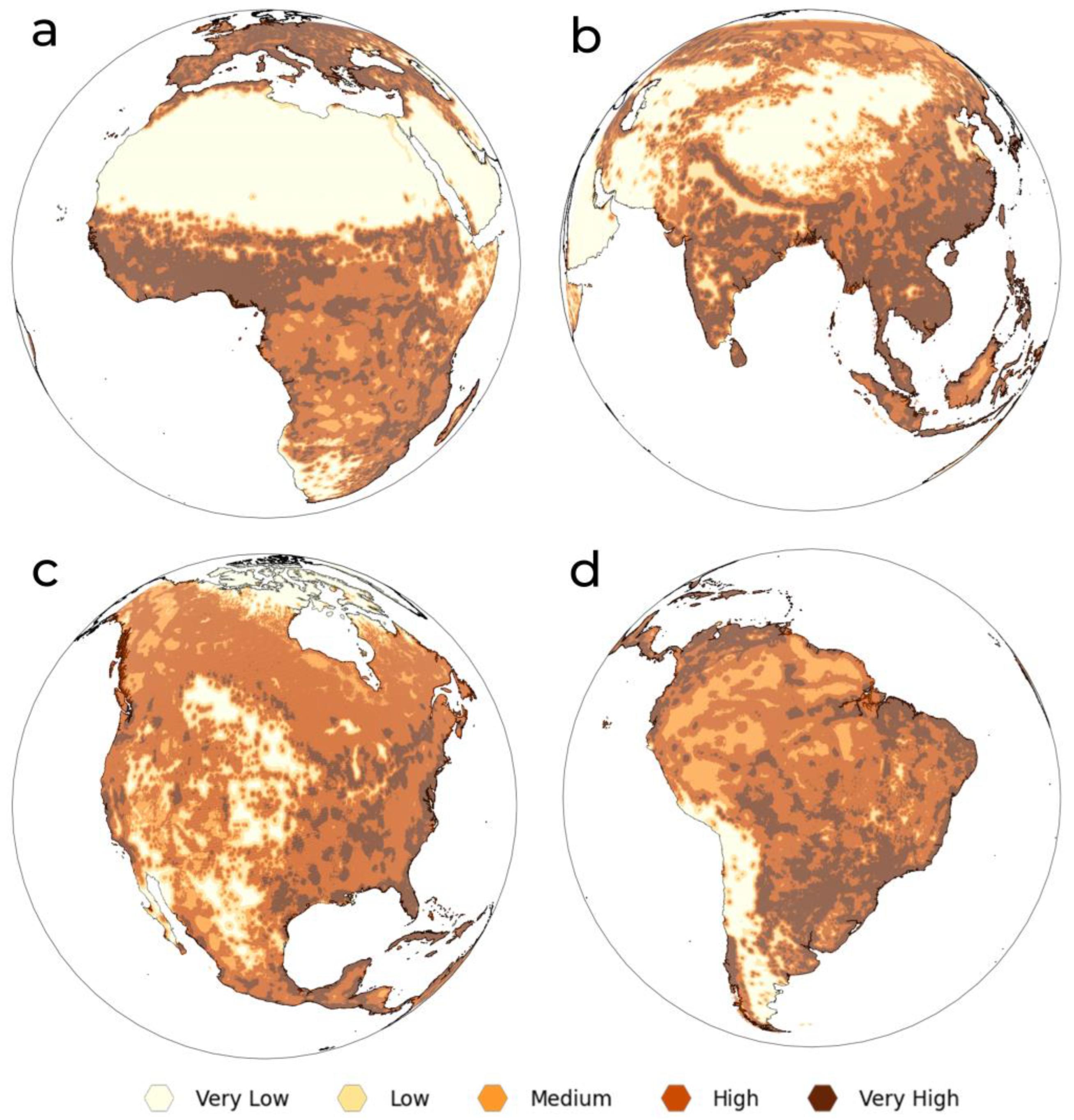
Weights were generated for each criterion to reflect the relative importance of the selected criteria in determining deforestation. While criteria weights in most GIS-based MCE methods can be determined by subject experts or stakeholders, this was not possible in this research study due to the global scope of the model’s application and resource limitations. Thus, the Automatic Weight Selection technique [75] was applied to generate the weights of importance, and values were normalized so the sum of all weights is equal to one. The technique is based on the comparison between locations of deforestation and random sampling sites using the Cohen’s d metric [76]. The obtained criterion weights are presented in Table 1. Based on the normalized criterion values and criterion weights, the Weighted Linear Combination (WLC) technique [77] was used to calculate the overall deforestation susceptibility scores for each hexagonal cell for deforestation. The obtained susceptibility scores were classified into five classes using the equal interval method. They were categorized as very low (0–0.2), low (0.21–0.4), medium (0.41–0.6), high (0.61–0.8), and very high (0.81–1) susceptibility to deforestation. The equal interval method was chosen to classify the susceptibility values due to its ability to create categories of equal sizes and for easy comparison. Figure 2 depicts the obtained global deforestation susceptibility output maps for different parts of the Earth.
2.6. Deforestation Scenarios
In this research study, three deforestation scenarios were designed and implemented to simulate forest land-cover change under different conditions: Business as Usual (BAU), Accelerated Deforestation (AD), and Sustainable Deforestation (SD) scenarios. The Business as Usual scenario assumes the historical rate of deforestation observed between 2010 and 2020 will continue in the future [78]. Further, deforestation inside protected areas is allowed due to ineffective implementation of forest conservation policies in some regions and to allow either for urbanization or agricultural expansion [79]. Research reveals that increased demand for forest products and services could amplify rates of deforestation by half in some parts of the world [80]. Therefore, the Accelerated Deforestation scenario assumes the rate of forest loss would be 50% higher than the current rate as well as loose implementation of environmental conservation policies. This represents a pessimistic deforestation scenario used to characterize forest-cover change under complete absence of forest management policies and lack of political commitments to reducing deforestation at the local and global levels. The Sustainable Deforestation scenario is the most optimistic and assumes a reduction in the current trend of deforestation by 50% through 2050 and 75% by 2100. Also, it encompasses the strict enforcement of forest conservation policies and programmes, and deforestation is restricted in protected areas under this scenario. Prior studies indicate the effective implementation of forest conservation policies and measures can positively impact global climate change. The research findings indicate reducing rates of deforestation by 50% could potentially reduce carbon emissions from land-cover change by 13 to 50 gigatons of carbon (GtC) [81,82].
Under each scenario, the model is constrained by the rate of deforestation at the country level and calculated using the 2010 and 2020 land-cover datasets. However, due to a lack of adequate data, the conversion of forest cover to water and snow and the process of reforestation are not considered.
2.7. Model Implementation and Evaluation
The spherical deforestation model was implemented in the Python programming language [83] using the DDGRID open-source library [84]. The model was implemented on a workstation with an Intel(R) Xeon(R) Gold 6128 CPU @ 3.40 GHz 3.39 GHz processor and 32 GB RAM, with the processing time for each scenario implementation varying between 81 and 88 h. The model was run for eight iterations with a temporal resolution of 10 years to simulate global deforestation between 2020 and 2100 () and for the three scenarios.
Model evaluation was performed using the relative operating characteristic (ROC) technique [85] and the Figure of Merit (FoM) [86]. ROC entails metrics for assessing the performance of binary classification with continuous output or rank order values [87,88]. ROC applies thresholds to generate a contingency table with four performance descriptors: true positives (TP), false negatives (FN), false positives (FP), and true negatives (TN) [89]. True positives (TP) correspond to changed forest cells correctly simulated as change by the model, false negatives (FN) are unchanged forest cells wrongly simulated as changed cells, false positives (FP) are changed forest cells the model was unable to simulate as changed cells, and true negatives (TN) are changed forest cells simulated as change but to the wrong land-cover class [90]. From the contingency table, the true positive rate (TPR) and false positive rate (FPR) can be calculated as follows:
By plotting the TPR on the vertical axis and FPR on the horizontal axis of the graph, the ROC curve and Area Under the Curve (AUC) metrics are obtained [91]. AUC values range between 0 and 1, where a larger value indicates higher model accuracy. Additionally, the simulation outputs are compared with actual land-cover datasets using the Figure of Merit (FoM) index which can be expressed as follows:
where the definition of the term misses is the same as false negatives, hits denote true positives, and false alarms are equivalent to false positives.
In this research study, global datasets for the period 2000–2010 were used for model calibration, and then global datasets for the period 2010–2020 were used for model validation. The AUC value obtained for the global spherical geographic deforestation model was 0.9 in the calibration phase and 0.87 in the validation phase. Other global geosimulation model applications in the scientific literature report AUC values ranging between 0.72 and 0.93 [92,93,94]. For the FoM metric, the value obtained was 36.5 for the model calibration and 29.9% during model validation. FoM values obtained in other global geosimulation models range between 19% and 43% [33,93]. Thus, the evaluation of the proposed modelling methodology yields commensurate values.
3. Results
3.1. Global and Regional Variations in Forest-Cover Change
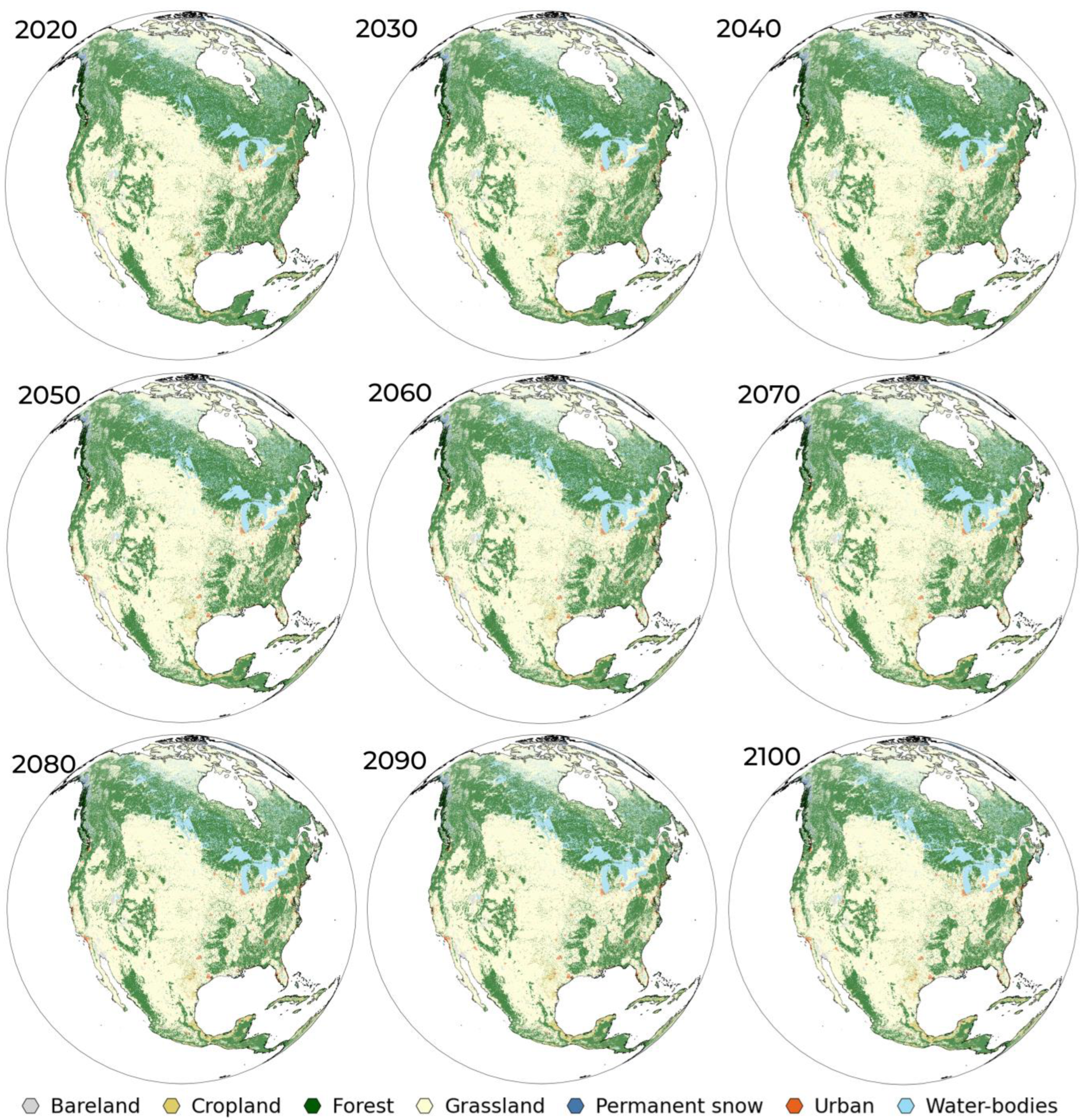
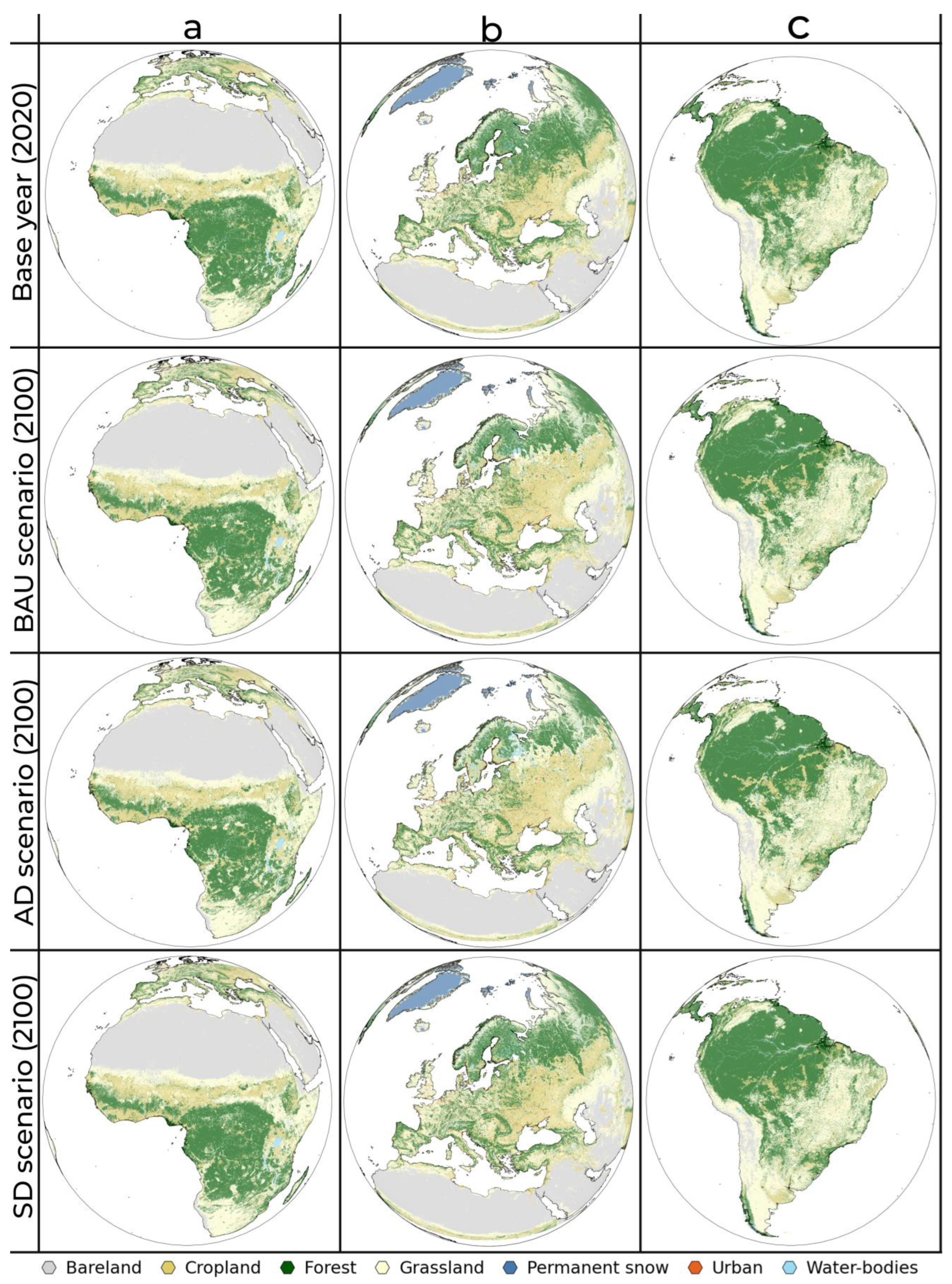
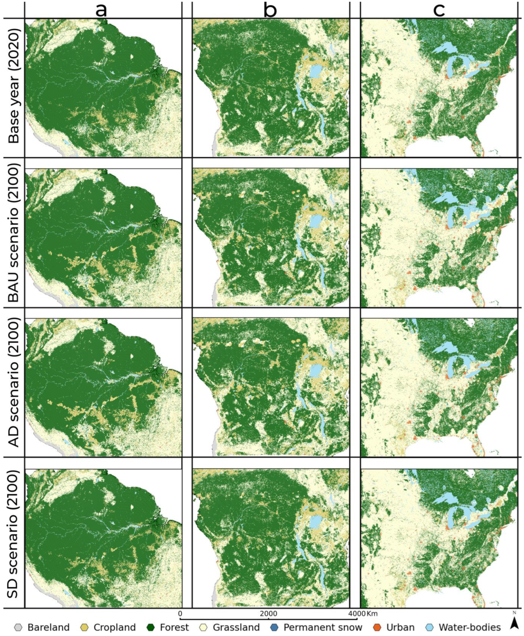
In 2020, forest covered 48 million km2 of the terrestrial Earth’s surface, corresponding to 35.6% of the global land area. The simulation results of deforestation are presented in Figure 3 for North America only as an illustration of detailed model outputs, and for each time step between 2020 and 2100 under the Accelerated Deforestation (AD) scenario. The obtained simulation outputs of deforestation under the different scenarios by the year 2100 compared with the base year 2020 are also presented for different parts of the globe in Figure 4.
Under the BAU scenario, the global forest extent shrinks to 43 million km2, decreasing by 5 million km2 between 2020 and 2100, which corresponds to an annual forest loss of 63 thousand km2 per year, about twice the size of the Netherlands. Approximately 10.5% of the forest extent in 2020 would be lost by the end of the 21st century based on the current trend of deforestation. Under the AD scenario, the global forest extent would decrease by 7.3 million km2, representing a forest loss of 15.3% by 2100. Conversely, the simulation results indicate 1.8 million km2 of the global forest area would be deforested by 2100 under the SD scenario, which represents a global forest loss of 3.7%. Figure 5 presents the global cumulative deforestation obtained for the three scenarios.
The simulation results also revealed marked differences in deforestation dynamics at the continental level. Table 2 presents summaries of the simulated forest-cover change per continent in the period between 2020 and 2100. At the continental level, Europe had the largest forest-cover loss with 1.9 million km2, corresponding to 15.5% of the continent’s forest extent in 2020, under the BAU scenario. The results further indicate forest loss in Europe would reach 2.7 million km2 under the AD scenario. It must however be noted that the Russian Federation which is considered part of Europe in this research accounts for 81.8% of Europe’s forest area in 2020. The simulation outputs also reveal considerable deforestation in North America with 1.02 million km2 of forest lost under the BAU scenario and 1.5 million km2 under the AD scenario. Forest losses in Africa, Asia, and South America are revealed to be 0.58 million km2, 0.66 million km2, and 0.76 million km2, respectively, under the BAU scenario. Figure 6 depicts simulated deforestation in 2100 compared to the base year for different forest regions across the globe under the three scenarios. The Amazon Forest, Congo Basin, and Eastern USA regions are presented here due to the extensive forest loss revealed by the simulation results.
Considerable differences in forest extent and rates of deforestation can be observed at the country level as well. The simulation results indicate the largest extent of deforestation would occur in the Russian Federation, Canada, the United States, and Brazil. Under the AD scenario, for example, 2.3 million km2, 0.81 million km2, 0.67 million km2, and 0.45 million km2 of forest area were lost in the Russian Federation, Canada, the United States, and Brazil, respectively, between 2020 and 2100. In relative terms, 17.4% of the forest in Canada and 20.3% of the forest in the United States would be lost by the end of the 21st century under this scenario. Moreover, there are several countries (over 50) with zero forest loss due to these countries having no forest cover, a lack of data, or the country being too small to capture the change in forest-cover change.
3.2. Forest Change in Protected Areas
In 2020, about 9.3 million km2 of the global forest was in protected areas, corresponding to 19.5% of the global forest extent. Simulation results indicate that this proportion, however, increases to 21.8%, 23%, and 20.2% by 2100 under the BAU, AD, and SD scenarios, respectively. The rate of deforestation within protected areas was significantly lower than the global rate as well. Between 2020 and 2100, only 0.03% of forests in protected areas were deforested under the BAU scenario, and 0.09% of forests in protected areas were deforested under the AD scenario. Conversely, the forest extent in protected areas under the SD scenario remained the same over the simulation period with no forest loss due to the restriction of deforestation in these areas. Table 3 presents the percentages of the share of forest extent located in protected areas at the continental level by 2100 and compared to the base year under the three scenarios. By 2100, 3.7 million km2 of forest in South America would be in protected areas under the BAU scenario, which represents 38.7% of all forest cover on the continent. This represents the largest share of protected forest area at the continental scale. In contrast, Oceania, North America, and Europe have the lowest percentage of protected forests at the continental level under all scenarios.
4. Discussion
Based on the simulation outputs, the global forest extent is projected to decrease over the coming decades, with the total forest extent in 2100 ranging between 46 and 40 million km2. However, the rate and magnitude of deforestation differ among the three scenarios and at the regional and country levels. The results indicate that Europe has the largest extent of deforestation by 2100; however, 85.4% of the deforested areas in Europe would occur in the Russian Federation. The results from the model presented in this research are comparable with other projections found in the literature with a range of outcomes varying between 25 million and 50 million km2 by 2100 under different scenarios [30,31,95]. However, as a caveat, simulation results from the presented model are largely dependent on the quality of the datasets utilized in the research. For instance, the rates of deforestation obtained at the country level for implementing the scenarios are derived from the available ESA-CCI land-cover datasets.
The pattern of forest-cover change observed also follows the process of deforestation as reported by prior studies [70,71]. From the simulation outputs, deforestation initially begins from the fringes of large forest regions and diminishes into the interior. This spatial pattern can be justified where forest regions in proximity to past forest disturbances, urban areas, water bodies, and road networks are more prone to deforestation. Over the course of the simulation run, regions initially covered by large forests become fragmented as deforestation spreads into the forest core. This pattern can be observed from the temporal simulation outputs presented in Figure 3.
While no forest management policies were explicitly included in the scenario design and implementation, the difference in results among the scenarios indicates the model can be utilized to assess different forest conservation policies. When properly implemented, protected areas can be used as effective forest conservation schemes to reduce deforestation. For instance, in the SD scenario where forest management policies are strictly implemented and deforestation in protected areas is not allowed, the simulation results reveal no loss of forest cover. However, such an outcome would be difficult to achieve due to the financial and human resources required to implement such a policy across large regions. However, the positive impact of protected areas on deforestation is proven by other studies in the scientific literature [63,96]. A research study [97] indicates that deforestation in protected areas accounted for only 5% of net forest loss between 2000 and 2021 in the Brazilian Amazon. Presently, protected areas are predominantly located in tropical regions of Africa, Asia, and South America, in contrast to the small proportion of protected forest areas in Europe and North America as obtained from the simulation results. According to [98], less than 10% of subtropical humid forests, temperate steppe and boreal coniferous forests largely found in Europe and North America are protected.
Despite the model’s capabilities in simulating deforestation at the global level and across different regions, the research study has some limitations. Improvements can be made to the model depending on the availability of quality and detailed global datasets to simulate land-cover change at finer spatial resolution as well as including more relevant criteria related to deforestation such as soil properties, climate variables, and forest type classification. By experimenting with different weighting methods such as Analytic Hierarchy Process (AHP) [99] or incorporating advanced spatial decision techniques such as Ordered Weighted Averaging (OWA) [100] and Logic Scoring of Preference (LSP) [101], the deforestation susceptibility analysis can be further improved for the SGA modelling framework. The selection of the relevant drivers of deforestation and generation of criterion weights can also be determined through engagement with subject experts and stakeholders in the model implementation phase of the research study. Considering the spatial heterogeneity and dynamics of the different drivers of deforestation across diverse regions and countries, implementation of region-specific economic or climate policies would be beneficial to improve the model. While only homogeneous forest was considered in this research, different forest types such as rainforest, boreal, deciduous, and mangrove, to name a few, can also be included in order to incorporate detailed characteristics of the different forest change dynamics. Additionally, the model can further be developed to incorporate multiple land-use/land-cover change types to reflect their different dynamics. This can assist in making informed decisions at country or regional levels and considering REDD+ [102] and OECD [103] concepts. Consideration of the natural regeneration of forests, reforestation, afforestation, and age of forested areas would be beneficial to enhance the proposed modelling approach. Moreover, with climate being one of the drivers of forest distribution, the inclusion of climate variables and scenarios can enhance the model’s ability to characterize future deforestation patterns and consider the effects of climate change. Augmenting computational power with more efficient code for the SGA model to run faster or on multiple processors when using global datasets would be another advantage.
5. Conclusions
This research study aimed to develop and implement a unique spherical geographic automata modelling approach that has been applied to represent and simulate the global deforestation process. Compared to existing geosimulation models and applications, the proposed model considers the curvature of the Earth’s surface, which is often ignored when modelling at the global level. For large-scale spatial applications, it is determined that the use of planar spatial models can produce very different results. Further, most global land-cover change models in the literature generally focus on simulating agricultural and urban land-use change, with few studies including deforestation.
Results from this research study indicate the spherical deforestation model can be successfully implemented to simulate the forest land-cover change process at the global level and under different “what-if” scenarios. Ultimately, the model is flexible and allows for further enhancements. Thus, the proposed deforestation modelling approach has a solid foundation to be used by intergovernmental entities, policymakers, ecologists, and researchers to support global forest management and conservation. With the United Nations (UN) Sustainable Development Goal (SDG) 15 set on promoting the sustainable use of terrestrial ecosystems and sustainable forest management and halting biodiversity loss, the spherical geographic deforestation model proposed in this research study can provide valuable insight and a spatial decision-support tool for achieving these targets.
Author Contributions
Conceptualization, Bright Addae and Suzana Dragićević; methodology, Bright Addae and Suzana Dragićević; software, Bright Addae; formal analysis, Bright Addae and Suzana Dragićević; investigation, Bright Addae and Suzana Dragićević; data curation, Bright Addae; writing—original draft preparation, Bright Addae and Suzana Dragićević; writing—review and editing, Bright Addae and Suzana Dragićević; supervision, Suzana Dragićević; funding acquisition, Suzana Dragićević. All authors have read and agreed to the published version of the manuscript.
Funding
This research was funded by the Natural Sciences and Engineering Research Council of Canada (NSERC) Discovery Grant number RGPIN-2023-04052.
Data Availability Statement
Publicly available datasets were used in this study. This data can be found at http://maps.elie.ucl.ac.be/CCI/viewer/download.php (accessed on 29 October 2022) (European Space Agency global land-cover data), https://www.globio.info/download-grip-dataset (accessed on 2 November 2022) (global roads dataset), https://www.protectedplanet.net/en/thematic-areas/wdpa?tab=WDPA (accessed on 10 July 2023) (protected areas dataset), https://gwis.jrc.ec.europa.eu/apps/country.profile/downloads (accessed on 15 February 2023) (global wildfire data), https://landscan.ornl.gov/ (accessed on 7 February 2023) (LandScan population density dataset), and https://earthexplorer.usgs.gov/ (accessed on 15 February 2023) (SRTM Digital Elevation Model).
Acknowledgments
The authors are thankful for the support of the Simon Fraser University Graduate Dean’s Entrance Scholarship (GDES) awarded to the first author and the Natural Sciences and Engineering Research Council of Canada (NSERC) Discovery Grant awarded to the second author. The authors are thankful for the valuable and constructive feedback from the five anonymous reviewers.
Conflicts of Interest
The authors declare no conflict of interest.
References
- Van Asselen, S.; Verburg, P.H. Land cover change or land-use intensification: Simulating land system change with a global-scale land change model. Glob. Chang. Biol. 2013, 19, 3648–3667. [Google Scholar] [CrossRef] [PubMed]
- Foley, J.A.; DeFries, R.; Asner, G.P.; Barford, C.; Bonan, G.; Carpenter, S.R.; Chapin, F.S.; Coe, M.T.; Daily, G.C.; Gibbs, H.K.; et al. Global consequences of land use. Science 2005, 309, 570–574. [Google Scholar] [CrossRef] [PubMed] [Green Version]
- Lambin, E.F.; Geist, H.J. Regional differences in tropical deforestation. Environ. Sci. Policy Sustain. Dev. 2003, 45, 22–36. [Google Scholar] [CrossRef]
- Hoang, N.T.; Kanemoto, K. Mapping the deforestation footprint of nations reveals growing threat to tropical forests. Nat. Ecol. Evol. 2021, 5, 845–853. [Google Scholar] [CrossRef]
- Curtis, P.G.; Slay, C.M.; Harris, N.L.; Tyukavina, A.; Hansen, M.C. Classifying drivers of global forest loss. Science 2018, 361, 1108–1111. [Google Scholar] [CrossRef]
- Brockerhoff, E.G.; Barbaro, L.; Castagneyrol, B.; Forrester, D.I.; Gardiner, B.; González-Olabarria, J.R.; Lyver, P.O.B.; Meurisse, N.; Oxbrough, A.; Taki, H.; et al. Forest biodiversity, ecosystem functioning and the provision of ecosystem services. Biodivers. Conserv. 2017, 26, 3005–3035. [Google Scholar] [CrossRef] [Green Version]
- Felipe-Lucia, M.R.; Soliveres, S.; Penone, C.; Manning, P.; van der Plas, F.; Boch, S.; Prati, D.; Ammer, C.; Schall, P.; Gossner, M.M.; et al. Multiple forest attributes underpin the supply of multiple ecosystem services. Nat. Commun. 2018, 9, 4839. [Google Scholar] [CrossRef] [PubMed] [Green Version]
- Food and Agriculture Organization of the United Nations. Global Gorest Resources Assessment 2020: Main Report; FAO: Rome, Iatly, 2020. [Google Scholar]
- Keenan, T.F.; Williams, C.A. The terrestrial carbon sink. Annu. Rev. Environ. Resour. 2018, 43, 219–243. [Google Scholar] [CrossRef]
- Pan, Y.; Birdsey, R.A.; Fang, J.; Houghton, R.; Kauppi, P.E.; Kurz, W.A.; Phillips, O.L.; Shvidenko, A.; Lewis, S.L.; Canadell, J.G.; et al. A large and persistent carbon sink in the world’s forests. Science 2011, 333, 988–993. [Google Scholar] [CrossRef] [Green Version]
- Ren, Y.; Lü, Y.; Comber, A.; Fu, B.; Harris, P.; Wu, L. Spatially explicit simulation of land use/land cover changes: Current coverage and future prospects. Earth-Sci. Rev. 2019, 190, 398–415. [Google Scholar]
- Vannier, C.; Cochrane, T.A.; Zawar Reza, P.; Bellamy, L. An analysis of agricultural systems modelling approaches and examples to support future policy development under disruptive changes in New Zealand. Appl. Sci. 2022, 12, 2746. [Google Scholar]
- Sun, J.; Zhang, Y.; Qin, W.; Chai, G. Estimation and simulation of forest carbon stock in Northeast China forestry based on future climate change and LUCC. Remote Sens. 2022, 14, 3653. [Google Scholar] [CrossRef]
- Yu, Z.; Ciais, P.; Piao, S.; Houghton, R.A.; Lu, C.; Tian, H.; Agathokleous, E.; Kattel, G.R.; Sitch, S.; Goll, D.; et al. Forest expansion dominates China’s land carbon sink since 1980. Nat. Commun. 2022, 13, 5374. [Google Scholar] [CrossRef] [PubMed]
- Bos, A.B.; De Sy, V.; Duchelle, A.E.; Herold, M.; Martius, C.; Tsendbazar, N.-E. Global data and tools for local forest cover loss and REDD+ performance assessment: Accuracy, uncertainty, complementarity and impact. Int. J. Appl. Earth Obs. Geoinf. 2019, 80, 295–311. [Google Scholar]
- Messier, C.; Puettmann, K.; Filotas, E.; Coates, D. Dealing with non-linearity and uncertainty in forest management. Curr. For. Rep. 2016, 2, 150–161. [Google Scholar] [CrossRef] [Green Version]
- Kura, A.L.; Beyene, D.L. Cellular automata Markov chain model based deforestation modelling in the pastoral and agro-pastoral areas of southern Ethiopia. Remote Sens. Appl. Soc. Environ. 2020, 18, 100321. [Google Scholar] [CrossRef]
- Moreno, N.; Quintero, R.; Ablan, M.; Barros, R.; Dávila, J.; Ramírez, H.; Tonella, G.; Acevedo, M.F. Biocomplexity of deforestation in the Caparo tropical forest reserve in Venezuela: An integrated multi-agent and cellular automata model. Environ. Model. Softw. 2007, 22, 664–673. [Google Scholar] [CrossRef]
- Vázquez-Quintero, G.; Solís-Moreno, R.; Pompa-García, M.; Villarreal-Guerrero, F.; Pinedo-Alvarez, C.; Pinedo-Alvarez, A. Detection and projection of forest changes by using the Markov chain model and cellular automata. Sustainability 2016, 8, 236. [Google Scholar] [CrossRef] [Green Version]
- Adhikari, S.; Southworth, J. Simulating forest cover changes of Bannerghatta National Park based on a CA-Markov model: A remote sensing approach. Remote Sens. 2012, 4, 3215–3243. [Google Scholar]
- Kucsicsa, G.; Dumitrică, C. Spatial modelling of deforestation in Romanian Carpathian Mountains using GIS and Logistic Regression. J. Mt. Sci. 2019, 16, 1005–1022. [Google Scholar] [CrossRef]
- Miranda-Aragón, L.; Treviño-Garza, E.J.; Jiménez-Pérez, J.; Aguirre-Calderón, O.A.; González-Tagle, M.A.; Pompa-García, M.; Aguirre-Salado, C.A. Modeling susceptibility to deforestation of remaining ecosystems in North Central Mexico with logistic regression. J. For. Res. 2012, 23, 345–354. [Google Scholar] [CrossRef]
- Monjardin-Armenta, S.A.; Plata-Rocha, W.; Pacheco-Angulo, C.E.; Franco-Ochoa, C.; Rangel-Peraza, J.G. Geospatial simulation model of deforestation and reforestation using multicriteria evaluation. Sustainability 2020, 12, 10387. [Google Scholar] [CrossRef]
- Takam Tiamgne, X.; Kanungwe Kalaba, F.; Raphael Nyirenda, V.; Phiri, D. Modelling areas for sustainable forest management in a mining and human dominated landscape: A geographical information system (GIS)-multi-criteria decision analysis (MCDA) approach. Ann. GIS 2022, 28, 343–357. [Google Scholar] [CrossRef]
- Mas, J.F.; Puig, H.; Palacio, J.L.; Sosa-López, A. Modelling deforestation using GIS and artificial neural networks. Environ. Model. Softw. 2004, 19, 461–471. [Google Scholar] [CrossRef]
- Ball, J.G.C.; Petrova, K.; Coomes, D.A.; Flaxman, S. Using deep convolutional neural networks to forecast spatial patterns of Amazonian deforestation. Methods Ecol. Evol. 2022, 13, 2622–2634. [Google Scholar] [CrossRef]
- Deadman, P.; Robinson, D.; Moran, E.; Brondizio, E. Colonist household decisionmaking and land-use change in the Amazon Rainforest: An agent-based simulation. Environ. Plan. B: Plan. Des. 2004, 31, 693–709. [Google Scholar]
- Manson, S.M.; Evans, T. Agent-based modeling of deforestation in southern Yucatán, Mexico, and reforestation in the Midwest United States. Proc. Natl. Acad. Sci. USA 2007, 104, 20678–20683. [Google Scholar] [CrossRef]
- Ellis, E.C.; Gauthier, N.; Klein Goldewijk, K.; Bliege Bird, R.; Boivin, N.; Díaz, S.; Fuller, D.Q.; Gill, J.L.; Kaplan, J.O.; Kingston, N.; et al. People have shaped most of terrestrial nature for at least 12,000 years. Proc. Natl. Acad. Sci. USA 2021, 118, e2023483118. [Google Scholar] [CrossRef]
- Cao, M.; Zhu, Y.; Quan, J.; Zhou, S.; Lü, G.; Chen, M.; Huang, M. Spatial sequential modeling and predication of global land use and land cover changes by integrating a global change assessment model and cellular automata. Earth’s Future 2019, 7, 1102–1116. [Google Scholar] [CrossRef] [Green Version]
- Li, X.; Chen, G.; Liu, X.; Liang, X.; Wang, S.; Chen, Y.; Pei, F.; Xu, X. A new global Land-use and land-cover change product at a 1-km resolution for 2010 to 2100 based on human–environment interactions. Ann. Am. Assoc. Geogr. 2017, 107, 1040–1059. [Google Scholar]
- Hu, X.; Næss, J.S.; Iordan, C.M.; Huang, B.; Zhao, W.; Cherubini, F. Recent global land cover dynamics and implications for soil erosion and carbon losses from deforestation. Anthropocene 2021, 34, 100291. [Google Scholar] [CrossRef]
- Chen, G.; Li, X.; Liu, X.; Chen, Y.; Liang, X.; Leng, J.; Xu, X.; Liao, W.; Qiu, Y.A.; Wu, Q.; et al. Global projections of future urban land expansion under shared socioeconomic pathways. Nat. Commun. 2020, 11, 537. [Google Scholar] [CrossRef] [PubMed] [Green Version]
- Gao, J.; O’Neill, B.C. Mapping global urban land for the 21st century with data-driven simulations and Shared Socioeconomic Pathways. Nat. Commun. 2020, 11, 2302. [Google Scholar] [CrossRef] [PubMed]
- Meiyappan, P.; Dalton, M.; O’Neill, B.C.; Jain, A.K. Spatial modeling of agricultural land use change at global scale. Ecol. Model. 2014, 291, 152–174. [Google Scholar] [CrossRef] [Green Version]
- Malczewski, J. A GIS-based approach to multiple criteria group decision-making. Int. J. Geogr. Inf. Syst. 1996, 10, 955–971. [Google Scholar] [CrossRef]
- Feng, H.; Lim, C.W.; Chen, L.; Zhou, X.; Zhou, C.; Lin, Y. Sustainable deforestation evaluation model and system dynamics analysis. Sci. World J. 2014, 2014, 106209. [Google Scholar] [CrossRef] [Green Version]
- Deribew, K.T.; Dalacho, D.W. Land use and forest cover dynamics in the North-eastern Addis Ababa, central highlands of Ethiopia. Environ. Syst. Res. 2019, 8, 8. [Google Scholar] [CrossRef] [Green Version]
- Gharaibeh, A.A.; Shaamala, A.H.; Ali, M.H. Multi-criteria evaluation for sustainable urban growth in An-Nuayyimah, Jordan; post war study. Procedia Manuf. 2020, 44, 156–163. [Google Scholar] [CrossRef]
- Addae, B.; Dragićević, S. Enabling geosimulations for global scale: Spherical geographic automata. Trans. GIS 2023, 27, 821–840. [Google Scholar] [CrossRef]
- Sahr, K.; White, D.; Kimerling, A.J. Geodesic discrete global grid systems. Cartogr. Geogr. Inf. Sci. 2003, 30, 121–134. [Google Scholar] [CrossRef] [Green Version]
- Addae, B.; Dragićević, S. Integrating multi-criteria analysis and spherical cellular automata approach for modelling global urban land-use change. Geocarto Int. 2022, 2152498. [Google Scholar] [CrossRef]
- European Space Agency. ESA CCI Land Cover Map Series 1992–2020; European Space Agency: Paris, France, 2022. [Google Scholar]
- Meijer, J.R.; Huijbegts, M.A.J.; Schotten, C.G.J.; Schipper, A.M. Global patterns of current and future road infrastructure. Environ. Res. Lett. 2018, 15, 064006. [Google Scholar] [CrossRef] [Green Version]
- United Nations Environment Programme World Conservation Monitoring Centre (UNEP-WCMC) and the International Union for Conservation of Nature (IUCN). The World Databse on Protected Areas (WDPA); UNEP-WCMC and IUCN: Cambridge, UK, 2023. [Google Scholar]
- Artés, T.; Oom, D.; de Rigo, D.; Durrant, T.H.; Maianti, P.; Libertà, G.; San-Miguel-Ayanz, J. A global wildfire dataset for the analysis of fire regimes and fire behaviour. Sci. Data 2019, 6, 296. [Google Scholar] [CrossRef] [PubMed] [Green Version]
- Rose, A.N.; McKee, J.J.; Sims, K.M.; Bright, E.A.; Reith, A.E.; Urban, M.L. LandScan 2019, 2019 ed.; Oak Ridge National Laboratory: Oak Ridge, TN, USA, 2020. [Google Scholar]
- United State Geological Survey. Digital Elevation—Shuttle Radar Topography Mission (SRTM) 1 Arc-Second Global; Earth Resources Observation and Science (EROS) Center: Sioux Falls, SD, USA, 2022. [Google Scholar]
- Sahr, K. Hexagonal discrete global GRID systems for geospatial computing. Arch. Photogramm. Cartogr. Remote Sens. 2011, 22, 363–376. [Google Scholar]
- Williams, B.A.; Venter, O.; Allan, J.R.; Atkinson, S.C.; Rehbein, J.A.; Ward, M.; Di Marco, M.; Grantham, H.S.; Ervin, J.; Goetz, S.J.; et al. Change in terrestrial human footprint drives continued loss of intact ecosystems. One Earth 2020, 3, 371–382. [Google Scholar] [CrossRef]
- Dinerstein, E.; Joshi, A.R.; Vynne, C.; Lee, A.T.L.; Pharand-Deschênes, F.; França, M.; Fernando, S.; Birch, T.; Burkart, K.; Asner, G.P.; et al. A “Global Safety Net” to reverse biodiversity loss and stabilize Earth’s climate. Sci. Adv. 2020, 6, eabb2824. [Google Scholar] [CrossRef]
- Gleeson, T.; Befus, K.M.; Jasechko, S.; Luijendijk, E.; Cardenas, M.B. The global volume and distribution of modern groundwater. Nat. Geosci. 2016, 9, 161–167. [Google Scholar] [CrossRef]
- Robertson, C.; Chaudhuri, C.; Hojati, M.; Roberts, S.A. An integrated environmental analytics system (IDEAS) based on a DGGS. ISPRS J. Photogramm. Remote Sens. 2020, 162, 214–228. [Google Scholar] [CrossRef]
- Sharma, P.; Thapa, R.B.; Matin, M.A. Examining forest cover change and deforestation drivers in Taunggyi District, Shan State, Myanmar. Environ. Dev. Sustain. 2020, 22, 5521–5538. [Google Scholar] [CrossRef] [Green Version]
- Hyandye, C.; Martz, L.W. A Markovian and cellular automata land-use change predictive model of the Usangu Catchment. Int. J. Remote Sens. 2017, 38, 64–81. [Google Scholar] [CrossRef]
- Jana, A.; Jat, M.K.; Saxena, A.; Choudhary, M. Prediction of land use land cover changes of a river basin using the CA-Markov model. Geocarto Int. 2022, 37, 14127–14147. [Google Scholar] [CrossRef]
- Grinand, C.; Vieilledent, G.; Razafimbelo, T.; Rakotoarijaona, J.-R.; Nourtier, M.; Bernoux, M. Landscape-scale spatial modelling of deforestation, land degradation, and regeneration using machine learning tools. Land Degrad. Dev. 2020, 31, 1699–1712. [Google Scholar] [CrossRef]
- Uusivuori, J.; Lehto, E.; Palo, M. Population, income and ecological conditions as determinants of forest area variation in the tropics. Glob. Environ. Chang. 2002, 12, 313–323. [Google Scholar] [CrossRef]
- Vieilledent, G.; Grinand, C.; Vaudry, R. Forecasting deforestation and carbon emissions in tropical developing countries facing demographic expansion: A case study in Madagascar. Ecol. Evol. 2013, 3, 1702–1716. [Google Scholar] [CrossRef] [PubMed] [Green Version]
- Adhikari, S.; Fik, T.; Dwivedi, P. Proximate causes of land-use and land-cover change in Bannerghatta National Park: A spatial statistical model. Forests 2017, 8, 342. [Google Scholar]
- Liang, E.; Wang, Y.; Piao, S.; Lu, X.; Camarero, J.J.; Zhu, H.; Zhu, L.; Ellison, A.M.; Ciais, P.; Peñuelas, J. Species interactions slow warming-induced upward shifts of treelines on the Tibetan Plateau. Proc. Natl. Acad. Sci. USA 2016, 113, 4380–4385. [Google Scholar] [CrossRef] [PubMed]
- Georg, M.; Sabine, M.; Jonas, V.; Sonam, C.; Duo, L. Highest treeline in the northern hemisphere found in Southern Tibet. Mt. Res. Dev. 2007, 27, 169–173. [Google Scholar]
- Barber, C.P.; Cochrane, M.A.; Souza, C.M.; Laurance, W.F. Roads, deforestation, and the mitigating effect of protected areas in the Amazon. Biol. Conserv. 2014, 177, 203–209. [Google Scholar] [CrossRef]
- Southworth, J.; Marsik, M.; Qiu, Y.; Perz, S.; Cumming, G.; Stevens, F.; Rocha, K.; Duchelle, A.; Barnes, G. Roads as drivers of change: Trajectories across the Tri-National frontier in MAP, the Southwestern Amazon. Remote Sens. 2011, 3, 1047–1066. [Google Scholar] [CrossRef] [Green Version]
- Bax, V.; Francesconi, W.; Quintero, M. Spatial modeling of deforestation processes in the Central Peruvian Amazon. J. Nat. Conserv. 2016, 29, 79–88. [Google Scholar] [CrossRef]
- González-González, A.; Villegas, J.C.; Clerici, N.; Salazar, J.F. Spatial-temporal dynamics of deforestation and its drivers indicate need for locally-adapted environmental governance in Colombia. Ecol. Indic. 2021, 126, 107695. [Google Scholar] [CrossRef]
- Doggart, N.; Morgan-Brown, T.; Lyimo, E.; Mbilinyi, B.; Meshack, C.K.; Sallu, S.M.; Spracklen, D.V. Agriculture is the main driver of deforestation in Tanzania. Environ. Res. Lett. 2020, 15, 034028. [Google Scholar] [CrossRef]
- Pendrill, F.; Gardner, T.A.; Meyfroidt, P.; Persson, U.M.; Adams, J.; Azevedo, T.; Bastos Lima, M.G.; Baumann, M.; Curtis, P.G.; De Sy, V.; et al. Disentangling the numbers behind agriculture-driven tropical deforestation. Science 2022, 377, eabm9267. [Google Scholar] [CrossRef] [PubMed]
- Gibbs, H.K.; Ruesch, A.S.; Achard, F.; Clayton, M.K.; Holmgren, P.; Ramankutty, N.; Foley, J.A. Tropical forests were the primary sources of new agricultural land in the 1980s and 1990s. Proc. Natl. Acad. Sci. USA 2010, 107, 16732–16737. [Google Scholar] [CrossRef]
- Broadbent, E.N.; Asner, G.P.; Keller, M.; Knapp, D.E.; Oliveira, P.J.C.; Silva, J.N. Forest fragmentation and edge effects from deforestation and selective logging in the Brazilian Amazon. Biol. Conserv. 2008, 141, 1745–1757. [Google Scholar] [CrossRef]
- Precinoto, R.S.; Prieto, P.V.; Figueiredo, M.d.S.L.; Lorini, M.L. Edges as hotspots and drivers of forest cover change in a tropical landscape. Perspect. Ecol. Conserv. 2022, 20, 314–321. [Google Scholar] [CrossRef]
- Brown, S.; Hall, M.; Andrasko, K.; Ruiz, F.; Marzoli, W.; Guerrero, G.; Masera, O.; Dushku, A.; DeJong, B.; Cornell, J. Baselines for land-use change in the tropics: Application to avoided deforestation projects. Mitig. Adapt. Strateg. Glob. Chang. 2007, 12, 1001–1026. [Google Scholar] [CrossRef] [Green Version]
- Hamunyela, E.; Brandt, P.; Shirima, D.; Do, H.T.T.; Herold, M.; Roman-Cuesta, R.M. Space-time detection of deforestation, forest degradation and regeneration in montane forests of Eastern Tanzania. Int. J. Appl. Earth Obs. Geoinf. 2020, 88, 102063. [Google Scholar] [CrossRef]
- Lima, A.; Silva, T.S.F.; Aragão, L.E.O.e.C.d.; Feitas, R.M.d.; Adami, M.; Formaggio, A.R.; Shimabukuro, Y.E. Land use and land cover changes determine the spatial relationship between fire and deforestation in the Brazilian Amazon. Appl. Geogr. 2012, 34, 239–246. [Google Scholar] [CrossRef]
- Veronesi, F.; Schito, J.; Grassi, S.; Raubal, M. Automatic selection of weights for GIS-based multicriteria decision analysis: Site selection of transmission towers as a case study. Appl. Geogr. 2017, 83, 78–85. [Google Scholar]
- Cohen, J. Statistical Power Analysis for the Behavioral Sciences; Lawrence Erlbaum Associates: Hillsdale, NJ, USA, 1977. [Google Scholar]
- Malczewski, J. On the use of weighted linear combination method in GIS: Common and best practice approaches. Trans. GIS 2000, 4, 5–22. [Google Scholar] [CrossRef]
- Galford, G.L.; Melillo, J.M.; Kicklighter, D.W.; Cronin, T.W.; Cerri, C.E.P.; Mustard, J.F.; Cerri, C.C. Greenhouse gas emissions from alternative futures of deforestation and agricultural management in the southern Amazon. Proc. Natl. Acad. Sci. USA 2010, 107, 19649–19654. [Google Scholar] [CrossRef] [PubMed]
- Prevedello, J.A.; Winck, G.R.; Weber, M.M.; Nichols, E.; Sinervo, B. Impacts of forestation and deforestation on local temperature across the globe. PLoS ONE 2019, 14, e0213368. [Google Scholar] [CrossRef] [PubMed] [Green Version]
- Ceccherini, G.; Duveiller, G.; Grassi, G.; Lemoine, G.; Avitabile, V.; Pilli, R.; Cescatti, A. Abrupt increase in harvested forest area over Europe after 2015. Nature 2020, 583, 72–77. [Google Scholar] [CrossRef]
- Kindermann, G.E.; Obersteiner, M.; Rametsteiner, E.; McCallum, I. Predicting the deforestation-trend under different carbon-prices. Carbon Balance Manag. 2006, 1, 15. [Google Scholar] [CrossRef] [PubMed] [Green Version]
- Mollicone, D.; Freibauer, A.; Schulze, E.D.; Braatz, S.; Grassi, G.; Federici, S. Elements for the expected mechanisms on ‘reduced emissions from deforestation and degradation, REDD’ under UNFCCC. Environ. Res. Lett. 2007, 2, 045024. [Google Scholar] [CrossRef]
- Van Rossum, G.; Drake, F. Python 3 Reference Manual; CreateSpace: Scotts Valley, CA, USA, 2009. [Google Scholar]
- Sahr, K. DGGRID Version 7.5. Available online: https://github.com/sahrk/DGGRID (accessed on 13 March 2023).
- Swets, J.A. Measuring the accuracy of diagnostic systems. Science 1988, 240, 1285–1293. [Google Scholar] [CrossRef] [Green Version]
- Pontius, R.G.; Boersma, W.; Castella, J.-C.; Clarke, K.; de Nijs, T.; Dietzel, C.; Duan, Z.; Fotsing, E.; Goldstein, N.; Kok, K.; et al. Comparing the input, output, and validation maps for several models of land change. Ann. Reg. Sci. 2008, 42, 11–37. [Google Scholar] [CrossRef] [Green Version]
- Mas, J.-F.; Soares Filho, B.; Pontius, R.G.; Farfán Gutiérrez, M.; Rodrigues, H. A suite of tools for ROC analysis of spatial models. ISPRS Int. J. Geo-Inf. 2013, 2, 869–887. [Google Scholar] [CrossRef] [Green Version]
- Gilmore Pontius, R.; Pacheco, P. Calibration and validation of a model of forest disturbancein the Western Ghats, India 1920–1990. GeoJournal 2004, 61, 325–334. [Google Scholar] [CrossRef]
- Camacho Olmedo, M.T.; Mas, J.-F.; Paegelow, M. Validation of Soft Maps Produced by a Land Use Cover Change Model. In Land Use Cover Datasets and Validation Tools: Validation Practices with QGIS; García-Álvarez, D., Camacho Olmedo, M.T., Paegelow, M., Mas, J.F., Eds.; Springer International Publishing: Cham, Switzerland, 2022; pp. 189–203. [Google Scholar]
- Pontius, R.G.; Parmentier, B. Recommendations for using the relative operating characteristic (ROC). Landsc. Ecol. 2014, 29, 367–382. [Google Scholar] [CrossRef]
- Paegelow, M. LUCC Based Validation Indices: Figure of Merit, Producer’s Accuracy and User’s Accuracy. In Geomatic Approaches for Modeling Land Change Scenarios; Camacho Olmedo, M.T., Paegelow, M., Mas, J.-F., Escobar, F., Eds.; Springer International Publishing: Cham, Switzerland, 2018; pp. 433–436. [Google Scholar]
- Čengić, M.; Steinmann, Z.J.N.; Defourny, P.; Doelman, J.C.; Lamarche, C.; Stehfest, E.; Schipper, A.M.; Huijbregts, M.A.J. Global maps of agricultural expansion potential at a 300 m resolution. Land 2023, 12, 579. [Google Scholar] [CrossRef]
- Li, X.; Zhou, Y.; Hejazi, M.; Wise, M.; Vernon, C.; Iyer, G.; Chen, W. Global urban growth between 1870 and 2100 from integrated high resolution mapped data and urban dynamic modeling. Commun. Earth Environ. 2021, 2, 201. [Google Scholar] [CrossRef]
- Li, X.; Yu, L.; Sohl, T.; Clinton, N.; Li, W.; Zhu, Z.; Liu, X.; Gong, P. A cellular automata downscaling based 1 km global land use datasets (2010–2100). Sci. Bull. 2016, 61, 1651–1661. [Google Scholar] [CrossRef] [Green Version]
- Chen, M.; Vernon, C.R.; Graham, N.T.; Hejazi, M.; Huang, M.; Cheng, Y.; Calvin, K. Global land use for 2015–2100 at 0.05° resolution under diverse socioeconomic and climate scenarios. Sci. Data 2020, 7, 320. [Google Scholar] [CrossRef]
- d’Annunzio, R.; Sandker, M.; Finegold, Y.; Min, Z. Projecting global forest area towards 2030. For. Ecol. Manag. 2015, 352, 124–133. [Google Scholar] [CrossRef] [Green Version]
- Qin, Y.; Xiao, X.; Liu, F.; de Sa e Silva, F.; Shimabukuro, Y.; Arai, E.; Fearnside, P.M. Forest conservation in Indigenous territories and protected areas in the Brazilian Amazon. Nat. Sustain. 2023, 6, 295–305. [Google Scholar] [CrossRef]
- Food and Agriculture Organization and The United Nations Environment Programme. The State of the World’s Forests 2020; FAO: Rome, Italy, 2020. [Google Scholar]
- Saaty, T.L. The Analytical Hierarchy Process; McGraw-Hill: New York, NY, USA, 1980. [Google Scholar]
- Yager, R.R. On ordered weighted averaging aggregation operators in multicriteria decisionmaking. IEEE Trans. Syst. Man Cybern. 1988, 18, 183–190. [Google Scholar] [CrossRef]
- Dujmovic, J.J.; Tré, G.D.; Weghe, N.V. LSP suitability maps. Soft Comput. 2010, 14, 421–434. [Google Scholar] [CrossRef]
- Angelsen, A. Policy Options to Reduce Deforestation. In REDD+: National Strategy and Policy Options; Angelsen, A., Brockhaus, M., Kanninen, M., Sills, E., Sunderlin, W.D., Wertz-Kanounnikoff, S., Eds.; Center for International Forestry Research (CIFOR): Bogor, Indonesia, 2009; pp. 125–138. [Google Scholar]
- Organisation for Economic Co-operation and Development (OECD). Rethinking Urban Sprawl: Moving Towards Sustainable Cities; OECD Publishing: Paris, France, 2018. [Google Scholar]
Figure 1.
Flowchart of the spherical deforestation model for simulating forest land-cover change at the global level.
Figure 1.
Flowchart of the spherical deforestation model for simulating forest land-cover change at the global level.

Figure 2.
Global deforestation susceptibility maps for (a) Africa, (b) Asia, (c) North America, and (d) South America.
Figure 2.
Global deforestation susceptibility maps for (a) Africa, (b) Asia, (c) North America, and (d) South America.

Figure 3.
Simulated deforestation for North America from 2020 to 2100 for each 10-year iteration under the Accelerated Deforestation (AD) scenario.
Figure 3.
Simulated deforestation for North America from 2020 to 2100 for each 10-year iteration under the Accelerated Deforestation (AD) scenario.

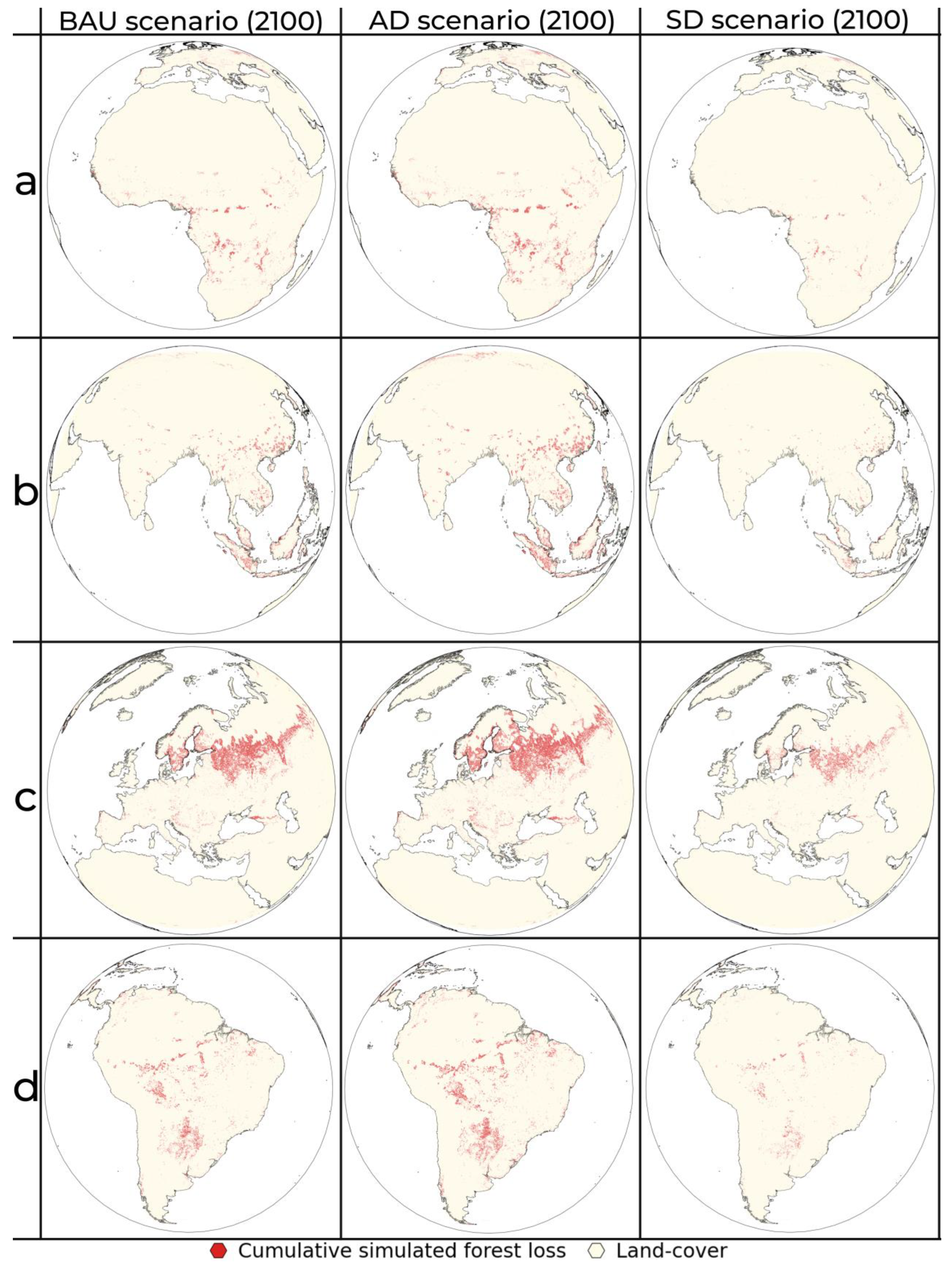
Figure 4.
Comparison of initial year 2020 forest cover with obtained simulation results of deforestation under Business as Usual (BAU), Accelerated Deforestation (AD), and Sustainable Deforestation (SD) scenarios for (a) Africa, (b) Europe, and (c) South America.
Figure 4.
Comparison of initial year 2020 forest cover with obtained simulation results of deforestation under Business as Usual (BAU), Accelerated Deforestation (AD), and Sustainable Deforestation (SD) scenarios for (a) Africa, (b) Europe, and (c) South America.

Figure 5.
Cumulative loss of forest land-cover between 2020 and 2100 based on the obtained simulation results under Business as Usual (BAU), Accelerated Deforestation (AD), and Sustainable Deforestation (SD) scenarios for (a) Africa, (b) Asia, (c) Europe, and (d) South America.
Figure 5.
Cumulative loss of forest land-cover between 2020 and 2100 based on the obtained simulation results under Business as Usual (BAU), Accelerated Deforestation (AD), and Sustainable Deforestation (SD) scenarios for (a) Africa, (b) Asia, (c) Europe, and (d) South America.

Figure 6.
Obtained simulation results of deforestation under Business as Usual (BAU), Accelerated Deforestation (AD), and Sustainable Deforestation (SD) scenarios compared to the base year for (a) Amazon Forest, (b) Congo Basin, and (c) Eastern USA.
Figure 6.
Obtained simulation results of deforestation under Business as Usual (BAU), Accelerated Deforestation (AD), and Sustainable Deforestation (SD) scenarios compared to the base year for (a) Amazon Forest, (b) Congo Basin, and (c) Eastern USA.


Table 1.
Selected criteria of deforestation with their respective susceptibility functions with rationale and criteria weights.
Table 1.
Selected criteria of deforestation with their respective susceptibility functions with rationale and criteria weights.
| Category | Deforestation Criteria | Susceptibility Functions | Rationale | Criteria Weights |
|---|---|---|---|---|
| Socioeconomic | Population density |  | Population density is an indicator for the concentration of human activities and thus closeness of possible deforestation processes. | 0.03418 |
| Terrain | Slope |  | Areas with gentle slopes are more suitable for land-use/land-cover change | 0.04323 |
| Elevation |  | Areas at lower elevation are more prone to deforestation as they are more accessible. | 0.17615 | |
| Proximity | Proximity to urban areas |  | Urbanization creates demand for land to support urban activities and infrastructure, thus entailing deforestation of adjacent forests. | 0.00824 |
| Proximity to major roads |  | Connection to transportation networks enhances deforestation by providing easy access to forest areas. | 0.04777 | |
| Proximity to water bodies |  | Water bodies provide access ways to forest regions and remote areas, thus increasing the possibility of deforestation. | 0.00645 | |
| Proximity to agriculture |  | Forest areas closer to agricultural land are more prone to deforestation due to expansion of farmlands and agroforestry. | 0.12282 | |
| Proximity to forest edges |  | Deforestation typically starts from the edges of existing forest regions as they are much easier to clear. | 0.38784 | |
| Proximity to past forest disturbances |  | Past forest disturbance areas are often precursors to future forest degradation or agricultural use. | 0.17331 |
Table 2.
Simulated forest-cover extent (in million km2) and percentage of cumulative forest lost (%) by continent between 2020 and 2100 under the Business as Usual (BAU), Accelerated Deforestation (AD), and Sustainable Deforestation (SD) scenarios.
Table 2.
Simulated forest-cover extent (in million km2) and percentage of cumulative forest lost (%) by continent between 2020 and 2100 under the Business as Usual (BAU), Accelerated Deforestation (AD), and Sustainable Deforestation (SD) scenarios.
| Continent | 2020 (106 km2) | Scenario | 2030 | 2040 | 2050 | 2060 | 2070 | 2080 | 2090 | 2100 | Lost (%) |
|---|---|---|---|---|---|---|---|---|---|---|---|
| Africa | 8.42 | BAU | 8.34 | 8.27 | 8.20 | 8.12 | 8.05 | 7.98 | 7.91 | 7.84 | 6.85 |
| AD | 8.31 | 8.20 | 8.09 | 7.98 | 7.88 | 7.77 | 7.67 | 7.57 | 10.08 | ||
| SD | 8.38 | 8.34 | 8.31 | 8.29 | 8.27 | 8.25 | 8.23 | 8.22 | 2.40 | ||
| Asia | 7.28 | BAU | 7.19 | 7.11 | 7.03 | 6.94 | 6.86 | 6.78 | 6.70 | 6.62 | 9.03 |
| AD | 7.15 | 7.02 | 6.90 | 6.78 | 6.66 | 6.55 | 6.43 | 6.32 | 13.18 | ||
| SD | 7.24 | 7.20 | 7.15 | 7.13 | 7.11 | 7.09 | 7.07 | 7.05 | 3.21 | ||
| Australia | 1.10 | BAU | 1.08 | 1.07 | 1.05 | 1.04 | 1.03 | 1.01 | 1.00 | 0.98 | 10.20 |
| AD | 1.07 | 1.05 | 1.03 | 1.01 | 0.99 | 0.97 | 0.95 | 0.93 | 14.97 | ||
| SD | 1.09 | 1.08 | 1.07 | 1.07 | 1.07 | 1.06 | 1.06 | 1.06 | 3.61 | ||
| Europe | 12.12 | BAU | 11.88 | 11.64 | 11.39 | 11.15 | 10.92 | 10.68 | 10.46 | 10.24 | 15.48 |
| AD | 11.75 | 11.39 | 11.03 | 10.68 | 10.34 | 10.02 | 9.70 | 9.40 | 22.45 | ||
| SD | 12.00 | 11.88 | 11.77 | 11.71 | 11.65 | 11.58 | 11.52 | 11.46 | 5.41 | ||
| North America | 7.97 | BAU | 7.83 | 7.70 | 7.57 | 7.45 | 7.33 | 7.20 | 7.08 | 6.96 | 12.74 |
| AD | 7.77 | 7.57 | 7.38 | 7.19 | 7.01 | 6.84 | 6.66 | 6.49 | 18.61 | ||
| SD | 7.90 | 7.84 | 7.77 | 7.74 | 7.71 | 7.67 | 7.64 | 7.61 | 4.51 | ||
| Oceania | 0.51 | BAU | 0.50 | 0.50 | 0.49 | 0.49 | 0.48 | 0.48 | 0.48 | 0.47 | 6.58 |
| AD | 0.50 | 0.49 | 0.49 | 0.48 | 0.47 | 0.47 | 0.46 | 0.46 | 9.67 | ||
| AD | 0.50 | 0.49 | 0.49 | 0.48 | 0.47 | 0.47 | 0.46 | 0.46 | 9.67 | ||
| South America | 10.40 | BAU | 10.30 | 10.20 | 10.10 | 10.00 | 9.91 | 9.82 | 9.73 | 9.64 | 7.33 |
| AD | 10.25 | 10.10 | 9.95 | 9.81 | 9.68 | 9.55 | 9.42 | 9.30 | 10.58 | ||
| SD | 10.35 | 10.30 | 10.25 | 10.22 | 10.20 | 10.18 | 10.15 | 10.13 | 2.65 |
Table 3.
Proportions of forest cover in percentages (%) located in protected areas by 2100 at the continental level under the Business as Usual (BAU), Accelerated Deforestation (AD), and Sustainable Deforestation (SD) scenarios and compared to the base year 2020.
Table 3.
Proportions of forest cover in percentages (%) located in protected areas by 2100 at the continental level under the Business as Usual (BAU), Accelerated Deforestation (AD), and Sustainable Deforestation (SD) scenarios and compared to the base year 2020.
| Scenario (%) | Africa | Asia | Australia | Europe | North America | Oceania | South America |
|---|---|---|---|---|---|---|---|
| Base year 2020 | 20.92 | 11.22 | 32.53 | 14.55 | 10.70 | 3.91 | 35.90 |
| BAU 2100 | 22.44 | 12.34 | 36.23 | 17.21 | 12.26 | 4.18 | 38.73 |
| AD 2100 | 23.25 | 12.85 | 38.26 | 18.76 | 13.15 | 4.33 | 40.14 |
| SD 2100 | 21.43 | 11.60 | 33.75 | 15.38 | 11.21 | 4.00 | 36.88 |
Disclaimer/Publisher’s Note: The statements, opinions and data contained in all publications are solely those of the individual author(s) and contributor(s) and not of MDPI and/or the editor(s). MDPI and/or the editor(s) disclaim responsibility for any injury to people or property resulting from any ideas, methods, instructions or products referred to in the content. |
© 2023 by the authors. Licensee MDPI, Basel, Switzerland. This article is an open access article distributed under the terms and conditions of the Creative Commons Attribution (CC BY) license (https://creativecommons.org/licenses/by/4.0/).
Share and Cite
MDPI and ACS Style
Addae, B.; Dragićević, S. Modelling Global Deforestation Using Spherical Geographic Automata Approach. ISPRS Int. J. Geo-Inf. 2023, 12, 306. https://doi.org/10.3390/ijgi12080306
AMA Style
Addae B, Dragićević S. Modelling Global Deforestation Using Spherical Geographic Automata Approach. ISPRS International Journal of Geo-Information. 2023; 12(8):306. https://doi.org/10.3390/ijgi12080306
Chicago/Turabian StyleAddae, Bright, and Suzana Dragićević. 2023. "Modelling Global Deforestation Using Spherical Geographic Automata Approach" ISPRS International Journal of Geo-Information 12, no. 8: 306. https://doi.org/10.3390/ijgi12080306
Note that from the first issue of 2016, this journal uses article numbers instead of page numbers. See further details here.