Article

Place-Centered Bus Accessibility Time Series Classification with Floating Car Data: An Actual Isochrone and Dynamic Time Warping Distance-Based k-Medoids Method

1
School of Resources and Environmental Engineering, Anhui University, Hefei 230601, China; +86-551-6386-1441
2
Anhui Province Key Laboratory of Wetland Ecosystem Protection and Restoration, Anhui University, Hefei 230601, China
3
Anhui Geographic Information Intelligence Technology and Engineering Center, Hefei 230001, China
4
Engineering Center for Geographic Information of Anhui Province, Hefei 230001, China
5
Anhui Mobile Communication Co., Ltd., Hefei 230001, China
*
Author to whom correspondence should be addressed.
ISPRS Int. J. Geo-Inf. 2023, 12(7), 285; https://doi.org/10.3390/ijgi12070285
Submission received: 3 May 2023 / Revised: 3 July 2023 / Accepted: 11 July 2023 / Published: 16 July 2023

Abstract

:
Classifying a time series is a fundamental task in temporal analysis. This provides valuable insights into the temporal characteristics of data. Although it has been applied to traffic flow and individual-centered accessibility analysis, it has yet to be applied to place-centered accessibility research. In this study, we have proposed an actual isochrone and dynamic time-wrapping distance-based k-medoids method and tested its applicability to a bus accessibility analysis. Using bus floating car data, our method calculated the actual isochrone area as an accessibility measurement and constructs an accessibility time series for each hexagonal geographical unit within the area of interest. We then calculated the dynamic time warp distance between the accessibility time series of pairwise geographical units and used these distances for k-medoid clustering. The optimized class number k was selected by considering the elbow method, silhouette score, and human examination. Our case study in Hefei, China demonstrates the feasibility of our method for accessibility time series classification. We also discovered that the resulting classes follow clear spatial patterns, indicating that different time series classes may be correlated with their spatial location. To our knowledge, this is the first time that such a classification method has been applied to place-centered accessibility time series analysis. Our data-driven method can inform place-centered accessibility in an era in which large quantities of spatiotemporal data like floating car data are available.

1. Introduction

Accessibility refers to the ability of individuals, goods, or services to reach their intended destination and acquire necessary services through a transportation network [1,2]. In the context of public transportation, accessibility serves as a crucial indicator of service quality and is essential for public transport planning. While static accessibility measurements consider network conditions, provider capability [3], and demand [4], researchers have long recognized the importance of a temporal perspective in accessibility [2,5]. The condition of the transport network, the density of the service schedule, and the amount of demand all contribute to fluctuations in accessibility. Accessibility research can be grouped into two categories: individual-centered and place-centered [2]. Although accessibility research that is centered on individuals has extensively incorporated a spatiotemporal framework [6,7,8], conventional place-centered accessibility methods have been mostly static [7,9,10]. Only in the last decade has place-centered accessibility research widely incorporated the temporal dynamics of traffic, service, and individual movement, thanks to new data from location-based services and floating car data (FCD) [11]. One group of studies introduced dynamic-describing variables for static accessibility measurements, such as a service schedule, in the accessibility measurement of London, UK, and Santa Barbara, California, USA [12,13]. Another group of studies calculated accessibility measurements for selected time frames and visualized these snapshots to facilitate the researcher’s geo-visual analysis of the accessibility dynamics, such as the research of Zhang et al., in ShenZhen, China [14]. However, studies in both groups are not entirely data-driven and may require subjectively selected metrics, statistical indices, time granularity, and visualization methods. As a result, the analysis could be time-consuming and may miss some of the underlying spatiotemporal patterns that the analyzer had not originally targeted. There is still a lack of a data-driven classification method for place-centered accessibility research based on the feature of the entire accessibility time series. This prevents scientists from classifying different locations in the area of interest into different classes based on their time series features. Such a classification task is fundamental to further spatiotemporal analysis.
This study aimed to classify a bus accessibility time series using a data-driven and quantitative methodology. The proposed method consisted of four steps. First, the study area was divided into uniform hexagonal geographical units, and actual isochrones were calculated repeatedly for each unit with predefined travel time thresholds and the time interval supported by the FCD of buses. This method used the area of the actual isochrone surface as the accessibility index of a certain timeframe and constructed an accessibility time series for each hexagonal unit. Second, the dynamic time warp (DTW) method was used to calculate distances between the accessibility time series of pairwise hexagonal units. Third, based on the pairwise distances, a k-medoids cluster method was used to classify these time series into a predefined number of classes. The research evaluated the classification results with quantitative metrics and thus chose the optimized class number. Finally, different time series groups were plotted on the map, and an explanation of their between-group differences and spatial distribution patterns is given, providing decision support for public transit policy makers. The analysis of the classification results demonstrates the capability of DTW in terms of detecting differences between accessibility time series in different regions and the feasibility of chaining DTW with the following classification algorithm.
To our knowledge, this study is the first to apply dynamic time warp methodology to the time series of actual isochrone-based bus service accessibility for spatial unit classification. With preset class numbers, this methodology can be fully data-driven, automatically analyzing bus transit data, classifying service regions by their accessibility time series, and helping bus managers find service abnormalities.
The remainder of this manuscript is structured as follows: Section 2 reviews the literature in terms of accessibility and its temporal-perspective-related research; Section 3 presents the methodology details of the proposed classification method; Section 4 presents a case study of Hefei’s bus accessibility and explains the observed phenomenon; Section 5 discusses the methodological choice made by this study during the case study and the potential implications; and Section 6 gives a short summary of this study.

2. Accessibility and Its Temporal Perspective

Accessibility is a measure of the ability of individuals, goods, or services to access their desired destination and obtain necessary services via a transportation network. It serves various purposes in different research regions, including facility location selection in Nanjing, China [15], public service evaluation in Tokyo, Japan [16], urban planning in Naples, Italy [17], and policy evaluation in Montreal, Canada, and also in China [18,19]. It also plays a significant role in the emerging fields of urban mobility sustainability [20] and environmental sustainability [21]. While accessibility has been used in urban planning since the 1920s [22], it was only explicitly defined by researchers in 1959 [23], and its definition and measurement remain multifaceted. There are two main categories of accessibility measurement: place-centered (passive accessibility) and individual-centered (active accessibility) [2]. Place-centered accessibility measurement considers accessibility as a characteristic of different locations, while individual-centered accessibility measurement views accessibility as a measure of how easily a person can reach their destination and obtain services [24,25].
A temporal perspective is a critical component of accessibility measurement, in addition to space and human perspectives [5,26]. Studies have established the importance of considering the temporal dimension in accessibility measurement. The temporal perspective can be realized by using time as a cost in the measurement [27,28] or by accounting for the temporal dynamics of attributes in the accessibility algorithm, such as varying traffic conditions or population in an area of interest. Accessibility measurements from an individual perspective have long incorporated temporal dynamics and constraints [5,7,8]. Additionally, some researchers have attempted to stochastically aggregate individual temporal dynamics. However, aggregating these individual-centered measures into place-centered measures has proven to be challenging [29]. Conventional location-based measures are static, but new data sources such as FCD offer researchers opportunities to capture the dynamic nature of accessibility [30,31,32]. With these data, some researchers have embedded static descriptive measurements of time series into accessibility time series [31], while others have created multiple accessibility snapshots for place-centered evaluation [32].
The isochrone map is a classical visual analytic tool used for measuring place-centered accessibility with temporal information and is widely employed in urban planning and public transport management [32]. It displays travel time from a given origin point in the area of interest through points, lines, or area isochrones [33,34,35]. As a passive accessibility measure [32], isochrone maps visualize time, which is often more relevant to passengers than distance [27]. They are particularly useful in time-related accessibility measurements [36] and can be readily integrated into spatiotemporal accessibility analysis [37,38]. The isochrone area can be viewed as a horizontal slice on three-dimensional space–time prisms, and its area can serve as a quantitative measure of accessibility at that specific time window. Isochrones are classified into three categories: ideal isochrones, free-flow isochrones, and actual isochrones [39].
The spatiotemporal analysis of place-centered accessibility, whether isochrone-based or not, typically involves visual analysis of preselected time windows or descriptive statistics of time series. However, the quantitative time series grouping method, which groups time series into different categories based on the similarity of their temporal dynamic patterns, has yet to be widely applied to place-centered accessibility analysis despite its prevalence in time series analysis [40] and traffic flow analysis [41], as well as its recent application in individual-centered accessibility analysis [42]. These methods differ from the latest time grouping method of Park et al. [43] in accessibility studies as their focus was on grouping within an accessibility time series rather than among different ones. Grouping time series could provide insight into the patterns of accessibility dynamics and facilitate abnormality detection. Dynamic time warping with nearest neighbor (DTW-NN) and rotation forest are two strong baseline time series grouping methods [40]. In recent years, deep-learning-based grouping methods such as multi-layer perceptron (MLP), convolutional neural network (CNN), echo state network (ESN), and an efficient federated distillation learning system for multitask time series classification have gained popularity [44,45]. To our knowledge, few studies have applied these grouping algorithms to place-centered accessibility and evaluated their applicability.

3. Methodology

Our place-centered accessibility time series grouping method with bus FCD contained four steps: data preparation and bus network construction, actual isochrone time series calculation, time series grouping, and validation (Figure 1).

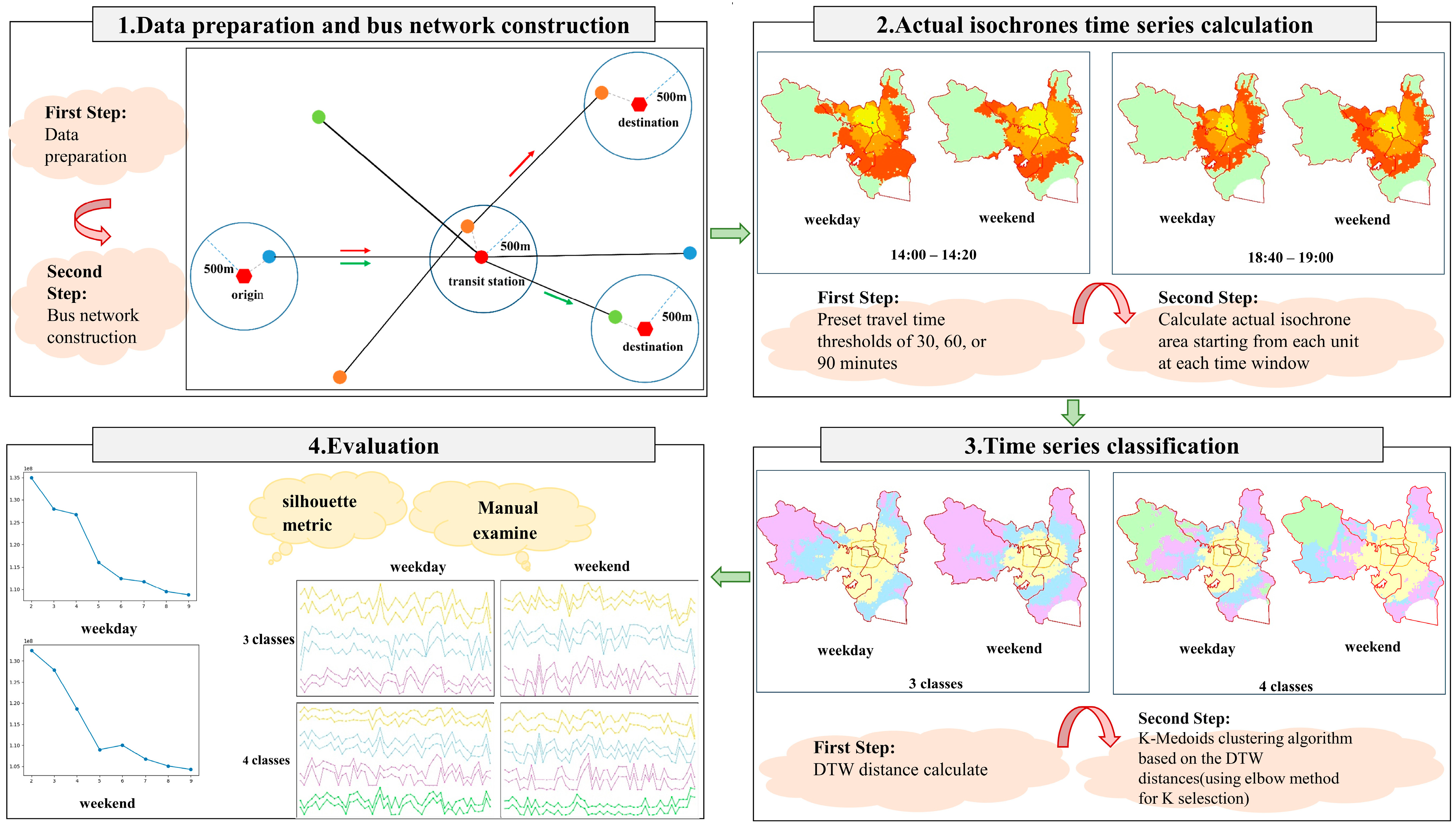
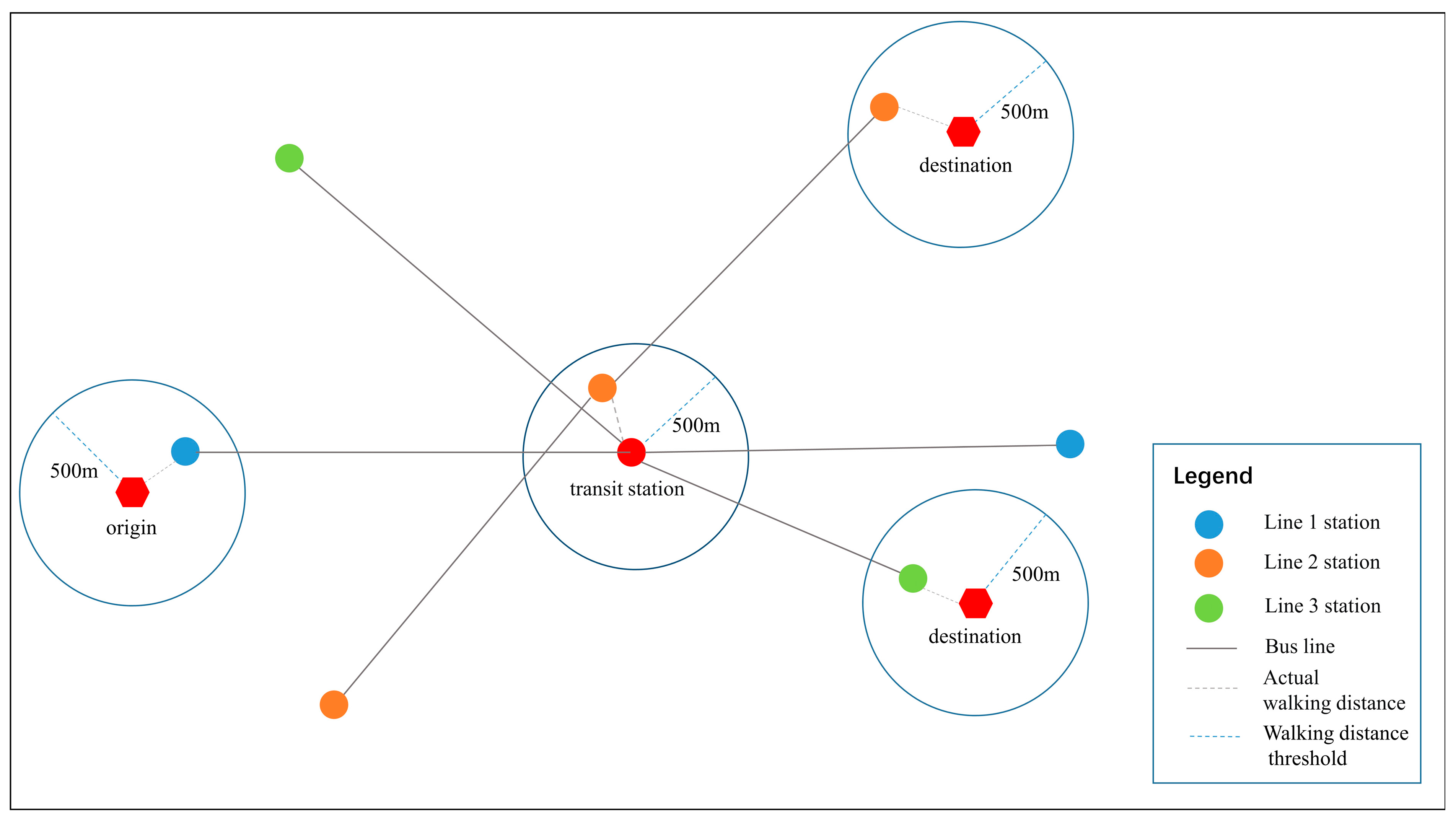
3.1. Data Preparation and Bus Network Construction

The data preparation and bus network construction process involved three data sets:
  • Road network data for the area of interest, which included the vertex, edge, and direction of roads.
  • Bus FCD for a period of interest, which included the location, record time, bus line, and service condition of each bus vehicle, often recorded at preset intervals.
  • Bus station data for the area of interest, which included the precise location and bus lines of all bus stations.
Due to limitations in the global positioning system (GPS) tracking and the obstruction of tall buildings in the city center, the precision of the bus FCD may have been compromised, and outliers may have been created. Therefore, the first step of our processing process involved snapping the bus FCD to the road network and removing outlier records. To achieve this, we employed a state-of-the-art snapping method that chained a hidden Markov model (HMM) and the Viterbi algorithm. Our method assumed that a bus vehicle moves at a constant speed between consecutive GPS sampling points and that the distribution of different bus speeds of a road segment within a short time window followed a Gaussian distribution [14,46]. Using this approach, we created a time series of bus speeds for each road edge by dividing the bus service hours into small time windows and calculating the expected speed in each time window accordingly. By doing so, we created a road network where each edge had a time series of bus speed. The original bus FCD may have introduced uncertainties in the speed calculation, as the location accuracy and update frequency were limited. However, since all of the FCD were processed by the same pipeline, the overall time series patterns should have remained comparable.
The bus network was then derived from the road network, with the bus stations as vertices and the edge representing either a bus traveling or the transit of passengers. The bus traveling edge merged road edges between bus stations and calculated the time series of travel time based on the time series of bus speed and length. There are two types of bus transit: between-station transit and within-station transit. The former refers to the transit that requires passengers to walk a certain distance. If the shortest path between two bus stations was shorter than a preset walking threshold, we established edges of between-station transit of opposite directions. The travel time of the transit edge was calculated based on its length and the pre-defined walking speed, for example 3.6 km/h. We neglected the time that a bus spends at each station, as the mean speed calculated from the FCD already accounts for the stopping delay. Within-station transit refers to the transit that is made within the same bus stop.
Edges representing within-station transit were also created. The time of within-station transit edge was set to half of the bus line interval at each time window, which could be derived from the FCD. The final bus network, as presented in Figure 2, consisted of bus station vertices, bus travel edges, within-station bus transit edges, and between-station bus transit edges. The travel time of each edge was calculated from the original road network and was dynamic.

3.2. Actual Isochrone Time Series Calculation

The dynamic travel time attribute of the bus network provided the basis for calculating dynamic actual isochrones, which reflected the actual traffic and service situation, as opposed to ideal isochrones. This study used the actual isochrone area as a measure of bus service accessibility and employed hexagonal geographical units for its calculation. Hexagonal units are preferred over square ones because they offer six spatially contiguous directions and exhibit smaller distance deviations between their boundary and centroid [47,48]. We calculated the origin destination (OD) matrix of travel time for each time window using the centroid of each hexagonal unit as the origin and destination, and we snapped the centroids to the nearest vertex of the bus network. If the nearest vertex was within the unit boundary, we neglected walking time to or from the vertex. Otherwise, we calculated walking time based on the distance from the nearest vertex to the hexagonal unit boundary and the preset walking speed. Equation (1) illustrates the modeling of the shortest bus travel time with one transfer between two hexagonal unit centroids.
T = O + W 1 + B 1 + S + W 2 + B 2 + D
where T denotes the time for one travel period with the bus; O denotes the time spent walking from the origin point to a nearby bus stop; W 1 denotes the time spent waiting for the first bus; B 1 denotes the time spent travelling on the first bus; S denotes the time for the bus transfer; W 2 denotes the time spent waiting for the second bus; B 2 denotes the time spent travelling on the second bus; D denotes the time spent walking from the last bus stop to the destination.
With multiple bus traveling OD matrices calculated per day, we could use them to calculate the actual isochrone area starting from each unit at each time window with a preset travel time threshold of 30, 60, or 90 min. The isochrone area could be calculated by their actual surface area or the count of geographical units. Using the isochrone area as a measurement, we could then acquire the time series of accessibility for each unit.

3.3. Time Series Classification

We could then employ DTW to calculate the elastic distance between the whole accessibility time series of each hexagonal unit pair. Given the two accessibility time series X = { x 1 , x 2 , , x n } and Y = { y 1 , y 2 , , y m } , their DTW distance was calculated using the following steps: First, we constructed a distance matrix D using the Euclidean distance as the basis function for the metric distance matrix D. The distance between the points x i and y j is denoted by D i , j , where i = 1 , 2 , , n and j = 1 , 2 , , m . Next, we calculated a warping path ( W ) subject to three conditions: the boundary condition, the continuity condition, and the monotonicity condition. The boundary condition required the calculation of the warping path to be performed from the first time point, i.e., from ( x 1 , y 1 ) , until the last time point, i.e., until the end of the point ( x n , y m ) . The continuity condition meant that only one time interval could be advanced at a time during matching, and there could be no crossing in the regularization path. Finally, the monotonic condition restricted the warping path to the next moment and not back. The warping path ( W ) is a sequence of indices w 1 , w 2 , , w K , where m a x ( n , m ) K n + m 1 .
We compared all of the dynamic regularization paths w i to find that with the smallest cumulative distance and defined this warping path as the dynamic regularization distance D T W X , Y between time series, see Equation (2):
D T W X , Y = m i n 1 K D w i
To obtain Equation (2), we solved the recurrent Equation (3):
γ i , j = D i , j + m i n γ i 1 , j γ i , j 1 γ i 1 , j 1
where γ 0,0 = . Then, γ i , j can be viewed as the sum of the base distance value of the current element and the minimum of the cumulative distance values of the 3 elements. The final γ n , m is the minimum cumulative cost of the DTW distance measure X and Y, i.e., D T W ( X , Y ) = γ ( n , m ) . The lower the DTW distance, the more similar the two accessibility time series.
Based on the DTW distances, we employed the k-medoids clustering algorithm [49], which consists of the following steps:
  • Determine the number of clusters K.
  • Randomly select K sample points from all data objects as the initial cluster center.
  • Assign the data into clusters where the nearest cluster centers are located based on the DTW distance of the time series.
  • Find the median member in each cluster, i.e., the member with the smallest average DTW distance from the remaining members and selecting that member as the new cluster center.
  • Repeat steps (3) and (4) and recalculating the centers of K clusters until the cluster centers remain unchanged or the maximum number of iterations set by the program is reached; then, the optimal clusters K for multi-centroid clustering based on dynamic time-wrapping distance are obtained.
Compared with k-means, the k-medoids method is more robust to outliers [50] and is better suited to a non-Euclidean distance where there is no clear definition of mean. It has already been employed in traffic flow [41] and urban planning research [50].
In this paper, a set of K was predefined, and the accessibility time-series classification result according to each K setting was calculated. All preset K and their classification results are also included in the next evaluation steps for K selection and result evaluation.

3.4. Evaluation

Since there were no predetermined class labels for the actual isochrone area time series, we could only quantitatively evaluate the classification using internal evaluation methods that were based only on the original data. To assess the quality of the classification results, we employed two internal metrics: the elbow method by within sum of DTW distance [51] and the Silhouette metric [52]. The silhouette metric is given by Equation (4):
S i = b i a i m a x a i , b i
where, S i is the silhouette metric of data object i , a i is the average distance from data object i to other data objects in the same cluster, and b i is the minimum value of the average distance from object i to objects in other clusters. The average S i of all data objects, called the silhouette score, provided an overall measure of the quality of clustering results, reflecting the validity and rationality of clustering. It ranges from −1 to 1. A higher average S i indicates better clustering results.
To further validate the clustering results, we manually examined the classification of accessibility time series by comparing time series plots within each class and between different classes. We also examined the size of each class and their statistical measurements to discover any abnormalities. The spatial distribution of the accessibility class distribution was also examined by categorically coloring the hexagonal units according to their class and presenting them in a thematic map of the area of interest. The classification thematic map provides a visual analytic tool for accessibility researchers to understand the spatial distribution of different time series classes and identify possible outlier groups.

4. Case Study: Hefei Bus Service

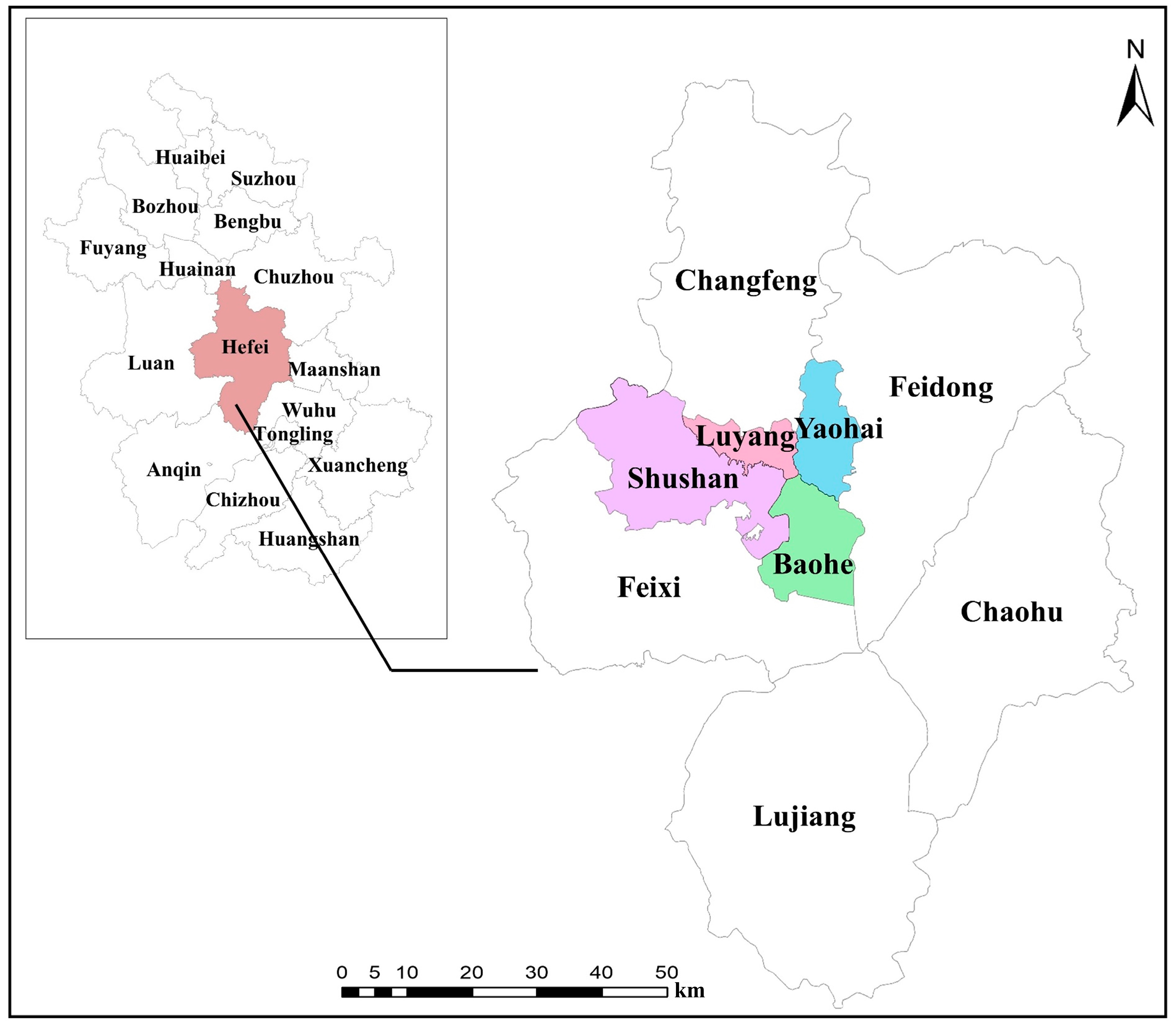
4.1. Study Area and Period

The study area, shown in Figure 3, is the urban area of Hefei, the capital of Anhui province in China, which is composed of four districts: Baohe, Shushan, Luyang, and Yaohai. This study utilized bus FCD that included the GPS location and time-stamped information of each bus vehicle, collected between 6 am and 11 pm for a week-long period from 2 November, 2020, to 8 November, 2020. Each day, the data set contained approximately 1 million points. The location updates occurred every minute, with some delays due to network connectivity issues. The Hefei metropolitan region spans over 1250 km2, with 406 daily bus lines, considering the upper and lower directions as separate bus lines, and around 3100 active vehicles. The bus network has over 2000 bus stations, with each stop accommodating an average of four bus lines. The road network data used in this research were derived from OpenStreetMap, while the bus station information was obtained from the bus company’s website and validated. The bus station information included the precise location and connected bus lines.

4.2. Data Preparation and Bus Network Construction

To accurately analyze the bus FCD, we utilized a Markov model (HMM) and Viterbi algorithm [53] to snap the data to Hefei’s road network and eliminate any outliers and inactive vehicles. Due to the limited availability of computational resources and the infrequent FCD updates, we set the time window to 20 min, resulting in 51 consecutive phases per day. Using the snapped FCD, we calculated the average bus speed for each road segment in each phase and reformed the road network with bus stations. The reform involved replacing the original vertices, mainly road intersections, with the vertices of bus stations. We constructed edges of the bus network representing the bus route between consecutive bus stations along a bus line and the passenger transit route. We represented within-station transit as edges connecting all possible transit bus lines passing a bus station and between-station transit edges connecting two possible bus station vertices. In accordance with the Urban Road Traffic Planning and Design Standards of China (GB50220-95), we set the between-station walking transit distance threshold to 500 m. Walking speed was set to 3.6 km/h based on analysis of mobile data from Anhui Mobile Communication Co., Ltd. The waiting time for each transit was set to half the arrival interval of each bus line at that bus station, derived by calculating possible bus arrival times using the road network with bus speed information. To construct the bus network, we employed OSMNX [54] and NetworkX [55] libraries and stored the resulting bus network in GraphML files for further processing.

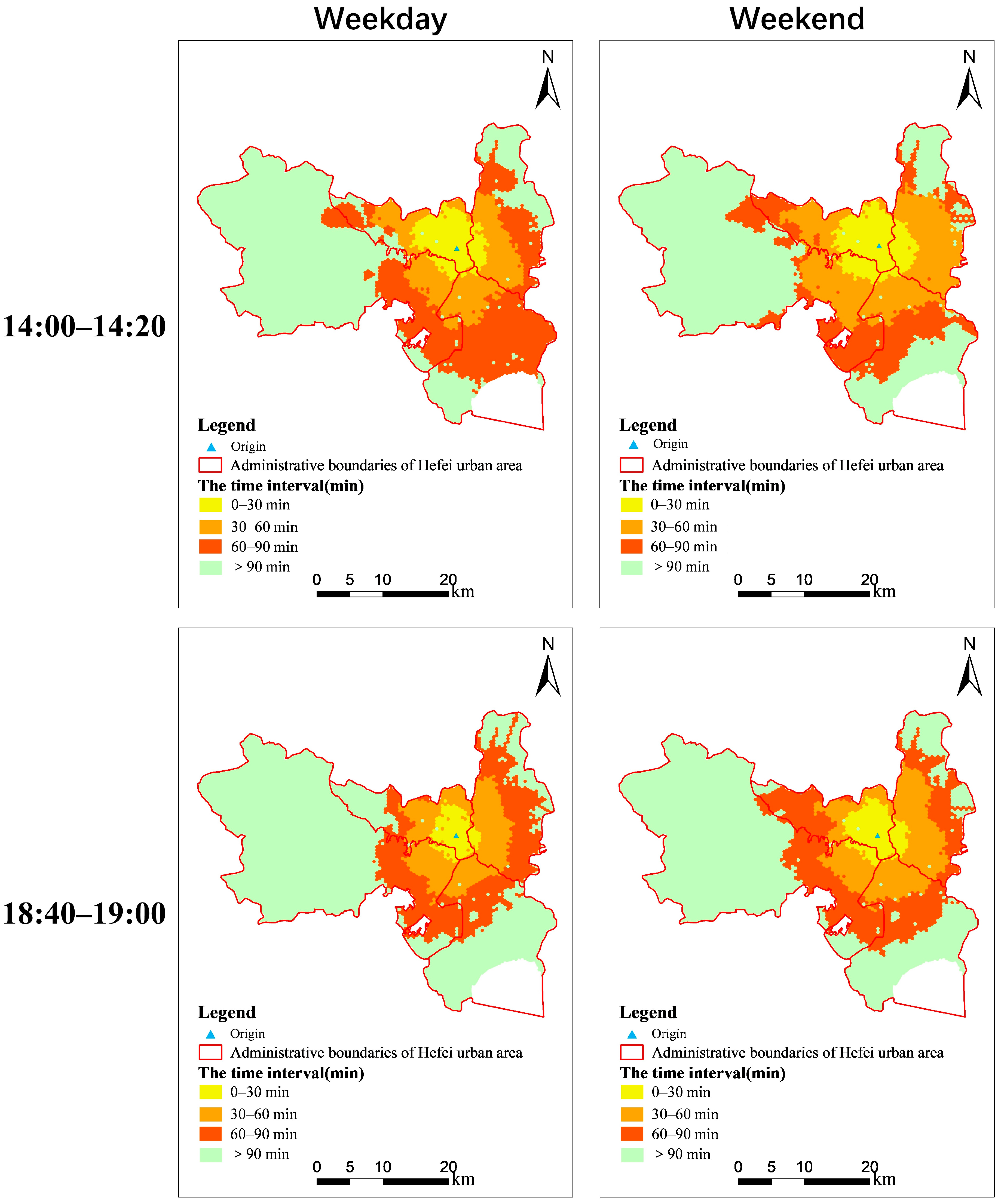
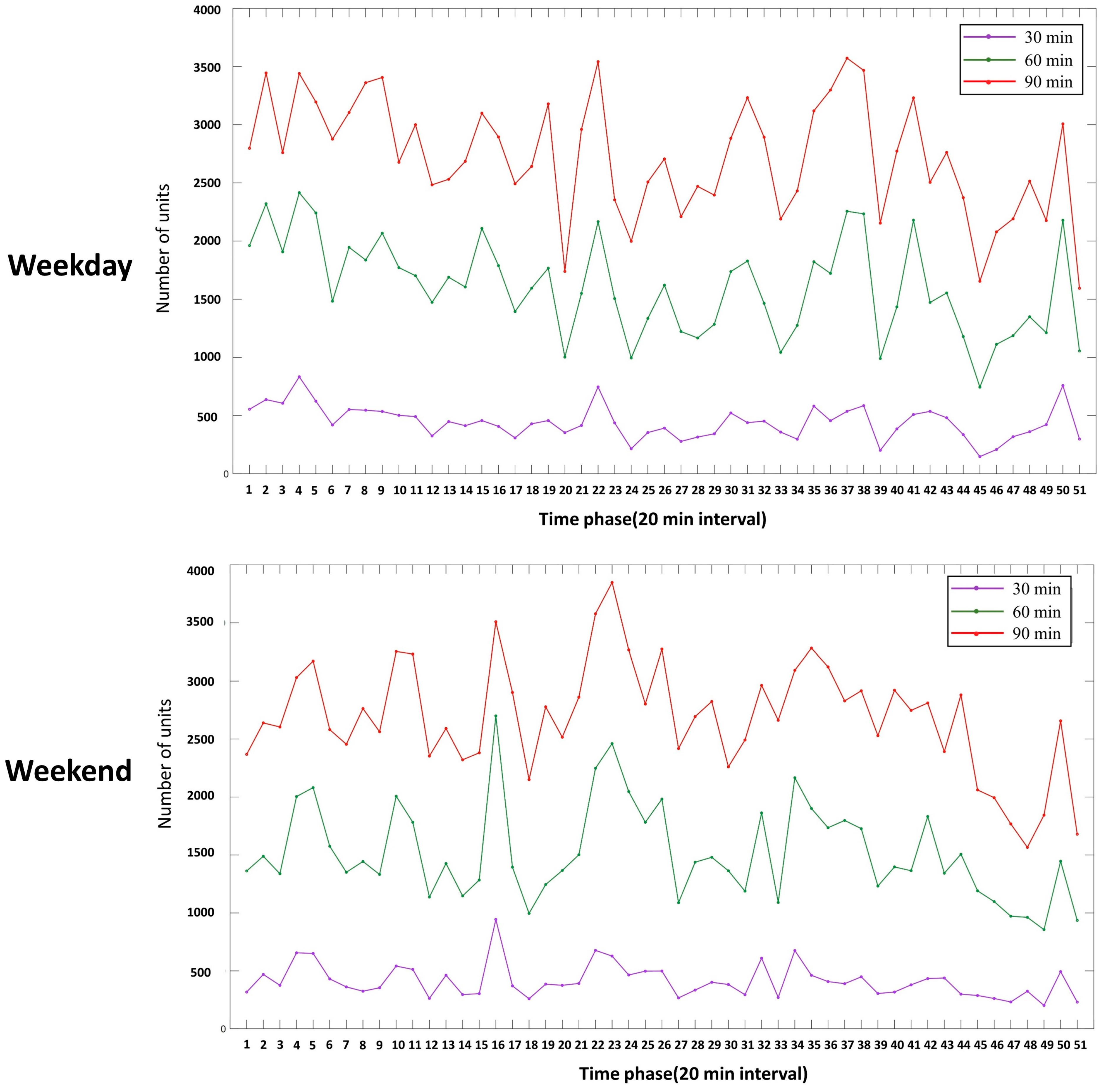
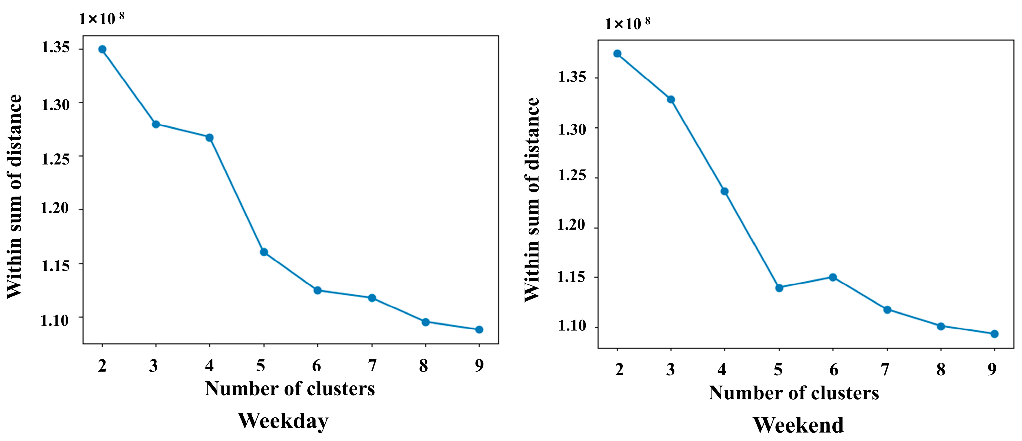
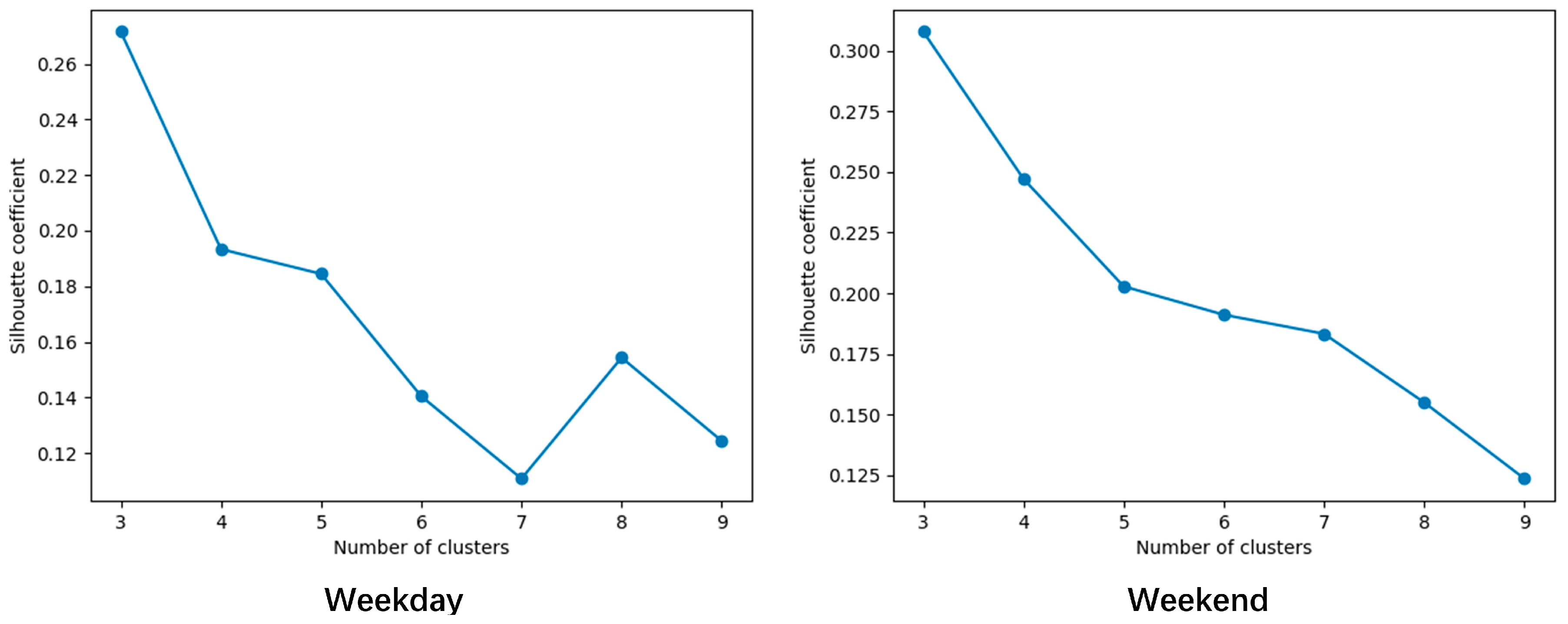
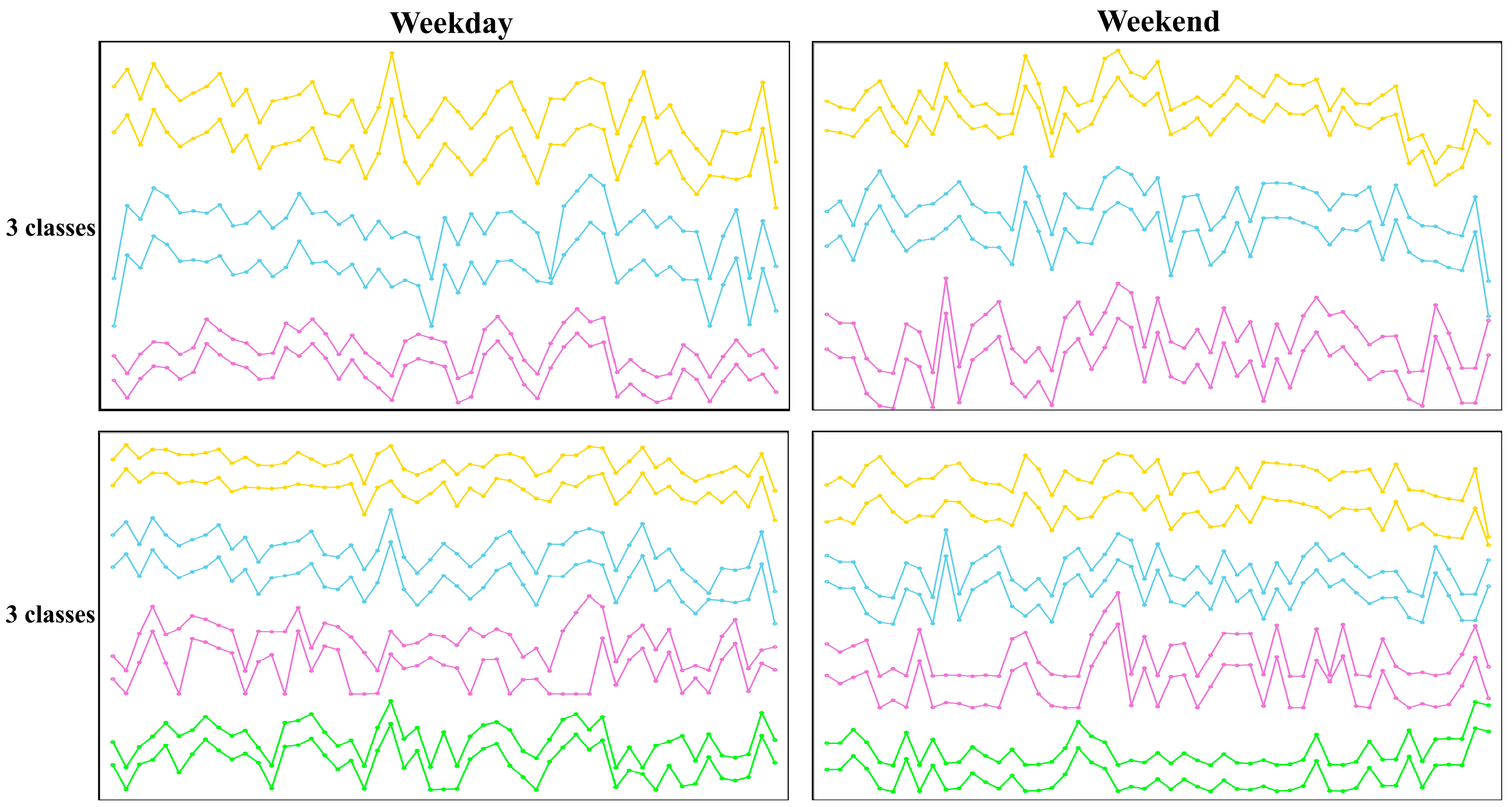
4.3. Actual Isochrone Time Series Calculation and Classification
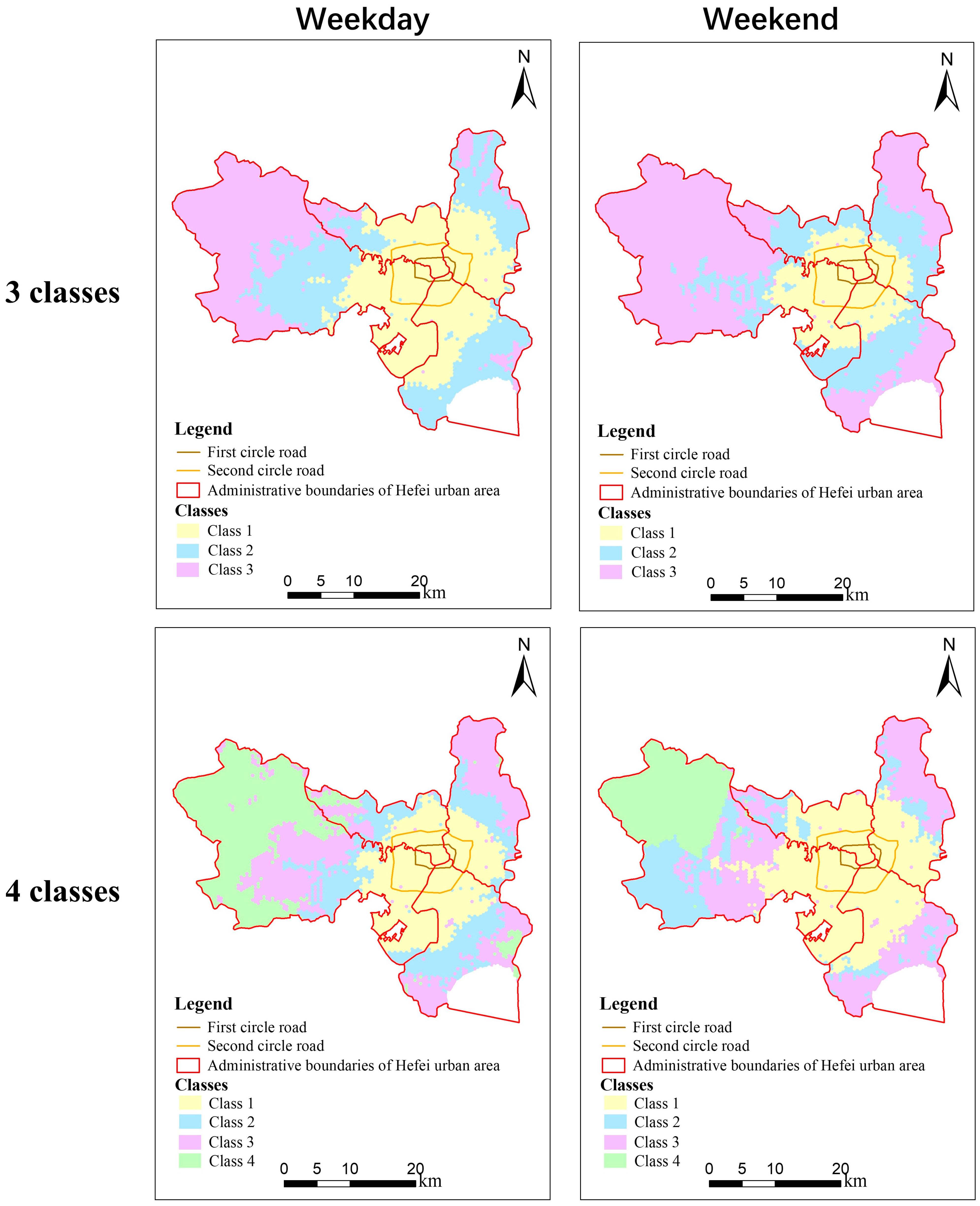
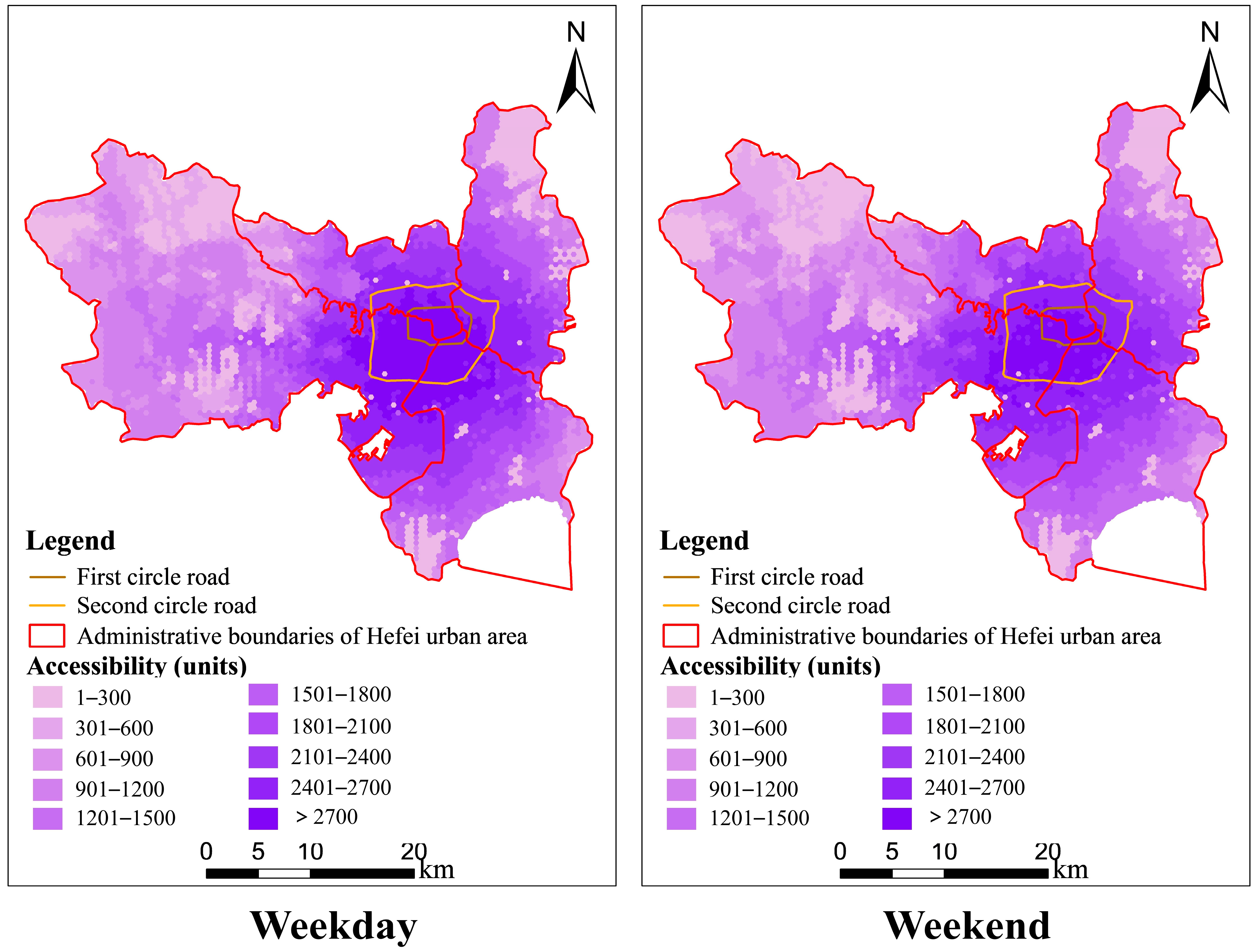
Due to data and computational resource constraints, we employed a 250 m hexagonal-based calculation scheme for the study. We calculated an origin destination (OD) matrix for every time window, with each hexagonal unit serving as both the origin and destination. We then aggregated the count of hexagonal units within 30, 60, and 90 min travel times for each hexagonal unit to measure its accessibility. To classify each hexagonal unit into different accessibility classes, we used a time series classification method based on dynamic time warping (DTW) and k-medoids. We optimized the number of classes using both the elbow method of within the sum of distance and silhouette score. The classification results were plotted on thematic maps, which colored each unit according to their class, to demonstrate whether there were spatial distribution patterns of time series classification.

4.4. Result

Figure 4 presents two isochrone maps, one for a weekday and another for a weekend, starting from one hexagonal unit. The resulting time series of accessibility values for this hexagonal unit is presented in Figure 5, which shows the 30, 60, and 90 min isochrone areas. The isochrone-based accessibility time series displays a fluctuation pattern that cannot be fully explained by peak and leisure times alone. While there were peak time windows in the morning, at noon, and in the late afternoon when accessibility declines, accessibility during most of the peak hours was not significantly lower than during leisure hours. An analysis of the bus FCD indicated that there were more active bus vehicles and lower bus arrival intervals during peak times compared to leisure times, which may explain why accessibility was not significantly lower during peak hours. However, once those extra peak hour buses arrived at their destination station, there was an immediate accessibility decline. Additionally, the bus service interval increase could explain the accessibility decline at noon when traffic conditions were not compromised. Weekend accessibility, with an average of 1435 units for the 90 min isochrone, was slightly lower than that of the weekday at 1493. However, their time series patterns were significantly different, as shown in Figure 5.
Figure 6 displays the sum of distance within classes as the classification number K increases. Figure 7 shows the silhouette score as K increases. The elbow method suggested an optimized K of 5 or 6, despite the elbow point in the diagram being vague. On the other hand, the silhouette score indicated 3 to be the best. The literature suggests that the silhouette score often performs best when evaluating cluster metrics [56,57]. The silhouette score for three class classifications was approximately 0.3, which is considered fair. Furthermore, we manually compared the time series diagrams of different classes and concluded that three classes were the best to account for the main time series classes and largely prevented overlapping between classes. The result of four classes was also presented as a reference, and Figure 8 shows two time series in each group with three and four classes on both weekdays and weekends. The time series is vertically offset from its original y-value in order to be presented together. Despite there being no dramatic time series shape difference, the time series shape of different classes in the three class classifications was distinguishable, but the shape differences in some patterns from different classes in the four class classifications for weekdays were not as obvious. The mean and median accessibility of each class were also significantly different, as shown in Table 1, which presents the all-day average accessibility for each class in the three class classifications.
Plotting hexagonal units with classes as different categories and with different colors revealed clear spatial patterns (Figure 9). These patterns differed from those of the whole-day median accessibility (Figure 10). The hexagonal units in class 1 compose a continuous surface in the city center, which is encircled by the first and second circle freeways. Moreover, class 2 encircles class 1, and class 3 encircles class 2. This pattern clearly indicates that the city center, suburbs, and outskirts have different accessibility time series features. Class 1 in the city center generally had a higher average accessibility evaluated by 30, 60, and 90 min isochrones, and it also presented different dynamic patterns, such as a clear accessibility peak at noon, while the other two classes did not. The city center, suburbs, and outskirts may exhibit distinct demographic characteristics, bus service provisions, and network profiles. These factors collectively contribute to the variations in accessibility time series features. Linear features were observed on the map, particularly towards the west direction, coinciding with two main routes where many bus stations are located. Holes within the continuous surface of class 1 can be explained by special ground situations, such as mountains, parks, and industrial fields, where both bus stations and bus lines are sparse. The four-class classification also presented some detailed spatial features of the suburban region. A noteworthy finding of the four-class classification was that the classification of weekdays and weekends differed significantly in the southwest part of the city. During the weekend, classes 2 and 3 no longer followed circular patterns. Unlike the continuous class 1, which remained in the city center during weekends, classes 2 and 3 were interwoven with both line and hole regions.
In summary, this study utilized an actual isochrone and dynamic time warping distance-based k-medoids method to classify bus accessibility time series in Hefei, China. The results of the case study, which yielded a fair silhouette score, demonstrated the feasibility of applying such a method to bus accessibility spatiotemporal analysis. The overall process was data-driven and provided valuable insights into the dynamic features of bus accessibility in Hefei. The strong spatial patterns observed in the distribution of different accessibility classes suggest a potential correlation between bus service and ground conditions, such as the situation of road networks and bus stations. Overall, the findings of this study contribute to a better understanding of Hefei’s bus service accessibility and its underlying influential factors in urban areas with the consideration of their temporal dynamics.

5. Discussion

The present study demonstrated the feasibility of actual isochrones and DTW distance-based k-medoid classification for analyzing the spatiotemporal accessibility of bus services. In this section, we discuss the methodological choices that were made in the case study of this study and their potential implications. The selection of the spatial and temporal granularity is a crucial step in any analysis of spatiotemporal data. In our study, we chose a geographical unit size of 250 m and constructed time series on a daily basis with each time window being 20 min. These choices were based on the frequency of bus FCD and the need to capture fine-grained spatiotemporal patterns. In our study, the upload frequency of each vehicle GPS device was 1 min. On average, a bus can travel 250 m for 1 min, so setting the geographical unit size to 250 m was reasonable. Park et al., made a similar decision [43]. The bus speed of each road segment was statistically determined, and a 20 min time window was required to robustly calculate the speed expectation. However, we acknowledge that different choices of unit size and time window may lead to different results, as indicated in previous studies [30,58], and further investigation is needed to understand the sensitivity of our method to these choices.
The selection of the number of classes (K) was another important parameter in our classification analysis. We used both the silhouette score and elbow method to evaluate the quality of clustering for different K values. In cases where the two methods produced conflicting results, we manually inspected the results. Our evaluation favored the silhouette score, which is consistent with previous benchmark studies [56,57]. Nonetheless, the choice of K is ultimately subjective and may require human intervention. Future studies could explore fully automatic K optimization methods, like that of Bholowalia et al. [51], for selecting the optimal K value. The k-medoid clustering method produces K classes at the same level, but a hierarchical classification may be more suitable for time series classification in the urban context, as some researchers have argued [42]. This could be an interesting direction for future research.
The DTW distance metric is influenced by both the shape of the time series and their Euclidean distance. Therefore, the accessibility time series of a given class should have similar shapes and similar absolute accessibility values. This explains why the mean accessibility of each class in our study was significantly different from each other. It also explains why some units with a similar all-day mean accessibility were assigned to different classes. Future work could focus on analyzing the dynamicity of accessibility time series alone.
This study focused solely on the analysis of bus floating car data (FCD). Consequently, the accessibility assessment was limited to the bus service alone. In reality, passengers also have the option to utilize subway services, which often have precise schedules and are not affected by road network traffic conditions. Exploring how to integrate subway schedule data with bus FCD in place-centered accessibility analysis presents an interesting avenue for future research. Additionally, in a multimodal public transit system like the one described, incorporating individual-centered accessibility into place-centered accessibility classification could offer valuable insights for future studies.
It is important to note that the case study conducted on the bus service in Hefei, presented in this research, serves primarily as an illustration of the proposed methodology. To the best of our knowledge, this methodology represents the first place-centered accessibility time series classification method. This unsupervised clustering approach offers two significant advantages for FCD-based and place-centered accessibility analysis. Firstly, it is data-driven, allowing for seamless integration into automated analysis pipelines and greatly reducing the need for manual intervention. This aspect is particularly beneficial in an era characterized by the prevalence of big data applicable to FCD. Secondly, the method enables spatiotemporal accessibility analysis based on features extracted from the entire time series, as opposed to selected snapshots. This approach enhances the objectivity and robustness of place-centered accessibility analysis. Furthermore, it enables the mapping of accessibility time series into categories and facilitates visual analysis of spatial distribution patterns. The findings from the case study conducted in Hefei, China, indicate that both accessibility and its time series feature exhibit spatial distribution patterns. This discovery suggests that the accessibility time series feature is a spatial phenomenon that may align with Tobler’s geographic first law. While our results revealed intriguing spatiotemporal patterns, we did not statistically investigate their correlations with the city’s geographical features, such as demographics and road networks. Exploring these correlations would be a fruitful avenue for future research.
The proposed accessibility time-series classification method also holds practical value for bus service planners and urban planners. It can assist practitioners in swiftly identifying abnormal zones, which may manifest as either temporal or spatial outliers. For instance, a class with a significantly smaller quantity of hexagonal units could indicate an accessibility time series outlier, while holes within the continuous class surface may suggest potential spatial outliers. The classification results of spatial units can also be readily utilized as raster data layers in subsequent spatial analysis processes. With access to longer periods of bus FCD, researchers could further develop new paradigms for bus transportation planning, location selection, urban planning, and policy evaluation.

6. Conclusions

This study has presented a novel method for bus accessibility time series classification based on actual isochrones and DTW distance-based k-medoid clustering using bus FCD. By constructing a bus service network with dynamic travel time using FCD and calculating the actual isochrones for each hexagonal geographical unit, the proposed method generates the accessibility time series of each unit and measures the pairwise distance between time series of different units using DTW. The results of the case study demonstrate the feasibility of the proposed method, with all the units being classified into three distinct classes based on their time series features. The classification result shows strong spatial cluster patterns and is well aligned with the underlying conditions of the bus network. This research has significant implications for place-centered accessibility research and provides a new data-driven method for public transit and urban planning practitioners. The proposed method has the potential to reveal the spatiotemporal dynamic patterns of bus accessibility by providing a precise classification of accessibility time series. Overall, this study fills a gap in the current literature and offers a valuable contribution to the field of time series classification in the context of bus accessibility analysis.

Author Contributions

Conceptualization, Chen Wang, Si-jia Zhao; methodology, Chen Wang; software, Chen Wang; validation, Si-jia Zhao; resources, Zong-qiang Ren, Qi Long; data processing, Si-jia Zhao; writing, Chen Wang; project administration, Chen Wang. All authors have read and agreed to the published version of the manuscript.

Funding

This work was supported in part by the National Natural Science Foundation of China under Grants 41901410, 42104036, 41701390, and 41906168; by the Open Research Fund Program of the Key Laboratory of Digital Mapping and Land Information Application Engineering, NASG, China, under Grant ZRZYBWD201905; by the Natural Science Foundation of Anhui Province under Grant 1908085QD161; and by the Hefei Municipal Natural Science Foundation No. 2021041.

Data Availability Statement

The sample data presented in this study are available on request from the corresponding author. The data are not publicly available due to their confidentiality.

Acknowledgments

The authors would like to thank Bei-ping Song and Bo Yang for their technical support in this project.

Conflicts of Interest

The authors declare no conflict of interest.

References

  1. Weibull, J.W. On the numerical measurement of accessibility. Environ. Plan A 1980, 12, 53–67. [Google Scholar] [CrossRef]
  2. Geurs, K.T.; Van Wee, B. Accessibility evaluation of land-use and transport strategies: Review and research directions. J. Transp. Geogr. 2004, 12, 127–140. [Google Scholar] [CrossRef]
  3. Ni, J.; Liang, M.; Lin, Y.; Wu, Y.; Wang, C. Multi-mode two-step floating catchment area (2SFCA) method to measure the potential spatial accessibility of healthcare services. ISPRS Int. J. Geo.-Inf. 2019, 8, 236. [Google Scholar] [CrossRef] [Green Version]
  4. Luo, J. Integrating the huff model and floating catchment area methods to analyze spatial access to healthcare services. Trans. GIS 2014, 18, 436–448. [Google Scholar] [CrossRef]
  5. Hägerstrand, T. Space, time and human conditions. Dyn. Alloc. Urban Space 1975, 3, 2–12. [Google Scholar]
  6. Weber, J.; Kwan, M.P. Bringing time back in: A study on the influence of travel time variations and facility opening hours on individual accessibility. Prof. Geogr. 2002, 54, 226–240. [Google Scholar] [CrossRef]
  7. Miller, H. Place-based versus people-based geographic information science. Geogr. Compass 2007, 1, 503–535. [Google Scholar] [CrossRef]
  8. Van Wee, B. Accessible accessibility research challenges. J. Transp. Geogr. 2016, 51, 9–16. [Google Scholar] [CrossRef] [Green Version]
  9. Neutens, T.; Delafontaine, M.; Scott, D.M.; De Maeyer, P. An analysis of day-to-day variations in individual space–time accessibility. J. Transp. Geogr. 2012, 23, 81–91. [Google Scholar] [CrossRef] [Green Version]
  10. Kwan, M.P. Beyond Space (as we Knew it): Toward Temporally Integrated Geographies of Segregation, Health, and Accessibility. Ann. Am. Assoc. Geogr. 2013, 103, 1078–1108. [Google Scholar] [CrossRef]
  11. Zook, M.; Kraak, M.J.; Ahas, R. Geographies of mobility: Applications of location- based data. Int. J. Geogr. Inf. Sci. 2015, 29, 1935–1940. [Google Scholar] [CrossRef]
  12. Ford, A.C.; Barr, S.L.; Dawson, R.J.; James, P. Transport accessibility analysis using GIS: Assessing sustainable transport in London. ISPRS Int. J. Geo.-Inf. 2015, 4, 124–149. [Google Scholar] [CrossRef] [Green Version]
  13. Lei, T.L.; Church, R.L. Mapping transit-based access: Integrating GIS, routes and schedules. Int. J. Geogr. Inf. Sci. 2010, 24, 283–304. [Google Scholar] [CrossRef]
  14. Zhang, T.; Dong, S.; Zeng, Z.; Li, J. Quantifying multi-modal public transit accessibility for large metropolitan areas: A time-dependent reliability modeling approach. Int. J. Geogr. Inf. Sci. 2018, 32, 1649–1676. [Google Scholar] [CrossRef]
  15. Yao, J.; Zhang, X.; Murray, A.T. Location optimization of urban fire stations: Access and service coverage. Comput. Environ. Urban. Syst. 2019, 73, 184–190. [Google Scholar] [CrossRef]
  16. Xia, T.; Song, X.; Zhang, H.; Song, X.; Kanasugi, H.; Shibasaki, R. Measuring spatio-temporal accessibility to emergency medical services through big GPS data. Health Place 2019, 56, 53–62. [Google Scholar] [CrossRef] [PubMed]
  17. Gaglione, F.; Gargiulo, C.; Zucaro, F.; Cottrill, C. Urban accessibility in a 15-minute city: A measure in the city of Naples, Italy. Transp. Res. Procedia 2022, 60, 378–385. [Google Scholar] [CrossRef]
  18. Páez, A.; Scott, D.M.; Morency, C. Measuring accessibility: Positive and normative implementations of various accessibility indicators. J. Transp. Geogr. 2012, 25, 141–153. [Google Scholar] [CrossRef]
  19. Shaw, S.L.; Fang, Z.; Lu, S.; Tao, R. Impacts of high speed rail on railroad network accessibility in China. J. Transp. Geogr. 2014, 40, 112–122. [Google Scholar] [CrossRef]
  20. Pavlyuk, D.; Spiridovska, N.; Yatskiv, I. Spatiotemporal dynamics of public transport demand: A case study of Riga. Transport 2020, 35, 576–587. [Google Scholar] [CrossRef]
  21. Lee, S.; Yoo, C.; Seo, K.W. Determinant factors of pedestrian volume in different land-use zones: Combining space syntax metrics with GIS-based built-environment measures. Sustain. Sci. 2020, 12, 8647. [Google Scholar] [CrossRef]
  22. Batty, M. Accessibility: In search of a unified theory. Environ. Plan. B Plan. Des. 2009, 36, 191–194. [Google Scholar] [CrossRef]
  23. Hansen, W.G. How accessibility shapes land use. J. Am. Inst. Plann. 1959, 25, 73–76. [Google Scholar] [CrossRef]
  24. Hu, Y.; Downs, J. Measuring and visualizing place-based space-time job accessibility. J. Transp. Geogr. 2019, 74, 278–288. [Google Scholar] [CrossRef]
  25. Cascetta, E.; Cartenì, A.; Montanino, M. A behavioral model of accessibility based on the number of available opportunities. J. Transp. Geogr. 2016, 51, 45–58. [Google Scholar] [CrossRef]
  26. Geurs, K.T.; Ritsema van Eck, J.R. Accessibility Measures: Review and Applications. Evaluation of Accessibility Impacts of Land-Use Transportation Scenarios, and Related Social and Economic Impact. RIVM Rapport 408505006. 2001. Available online: https://www.researchgate.net/publication/46637359_Accessibility_Measures_Review_and_Applications (accessed on 2 May 2023).
  27. Ullah, R.; Kraak, M. An alternative method to constructing time cartograms for the visual representation of scheduled movement data. J. Maps 2015, 11, 674–687. [Google Scholar] [CrossRef] [Green Version]
  28. Bertolini, L.; Le Clercq, F.; Kapoen, L. Sustainable accessibility: A conceptual framework to integrate transport and land use plan-making. Two test-applications in the Netherlands and a reflection on the way forward. Transp. Policy 2005, 12, 207–220. [Google Scholar] [CrossRef]
  29. Horner, M.W.; Downs, J.A. Integrating people and place: A density-based measure for assessing accessibility to opportunities. JTLU 2014, 7, 23–40. [Google Scholar] [CrossRef] [Green Version]
  30. Benenson, I.; Ben-Elia, E.; Rofé, Y.; Geyzersky, D. The benefits of a high-resolution analysis of transit accessibility. Int. J. Geogr. Inf. Sci. 2017, 31, 213–236. [Google Scholar] [CrossRef]
  31. Kujala, R.; Weckström, C.; Mladenović, N.; Saramäki, J. Travel times and transfers in public transport: Comprehensive accessibility analysis based on Pareto-optimal journeys. Comput. Environ. Urban. Syst. 2018, 67, 41–54. [Google Scholar] [CrossRef]
  32. Li, Q.; Zhang, T.; Wang, H.; Zeng, Z. Dynamic accessibility mapping using floating car data: A network-constrained density estimation approach. J. Transp. Geogr. 2011, 19, 379–393. [Google Scholar] [CrossRef]
  33. Moya-Gómez, B.; Salas-Olmedo, M.H.; García-Palomares, J.C.; Gutiérrez, J. Dynamic accessibility using big Data: The role of the changing conditions of network congestion and destination attractiveness. Netw. Spat. Econ. 2018, 18, 273–290. [Google Scholar] [CrossRef] [Green Version]
  34. Efentakis, A.; Grivas, N.; Lamprianidis, G.; Magenschab, G.; Pfoser, D. Isochrones, traffic and DEMOgraphics. In Proceedings of the 21st ACM SIGSPATIAL International Conference on Advances in Geographic Information Systems, Orlando, FL, USA, 5–8 November 2013; pp. 558–561. [Google Scholar] [CrossRef] [Green Version]
  35. Marciuska, S.; Gamper, J. Determining Objects within Isochrones in Spatial Network Databases. ADBIS 2010, 10, 392–405. [Google Scholar] [CrossRef]
  36. Wang, L.; Liu, Y.; Liu, Y.; Sun, C.; Huang, Q. Use of isochrone maps to assess the impact of high-speed rail network development on journey times: A case study of Nanjing city, Jiangsu province, China. J. Maps 2016, 12, 514–519. [Google Scholar] [CrossRef] [Green Version]
  37. O’Sullivan, D.; Morrison, A.; Shearer, J. Using desktop GIS for the investigation of accessibility by public transport: An isochrone approach. Int. J. Geogr. Inf. Sci. 2000, 14, 85–104. [Google Scholar] [CrossRef]
  38. van den Berg, J.; Köbben, B.; van der Drift, S.; Wismans, L. Towards a Dynamic Isochrone Map: Adding Spatiotemporal Traffic and Population Data. In Lecture Notes in Geoinformation and Cartography; Springer International Publishing: Cham, Switzerland, 2018; pp. 195–209. [Google Scholar] [CrossRef]
  39. Śleszyński, P.; Olszewski, P.; Dybicz, T.; Goch, K.; Niedzielski, M.A. The ideal isochrone: Assessing the efficiency of transport systems. Res. Transp. Bus. Manag. 2023, 46, 100779. [Google Scholar] [CrossRef]
  40. Bagnall, A.; Lines, J.; Bostrom, A.; Large, J.; Keogh, E. The great time series classification bake off: A review and experimental evaluation of recent algorithmic advances. Data Min. Knowl. Disc. 2017, 31, 606–660. [Google Scholar] [CrossRef] [PubMed] [Green Version]
  41. Li, M.; Zhu, Y.; Zhao, T.; Angelova, M. Weighted dynamic time warping for traffic flow clustering. Neurocomputing 2022, 472, 266–279. [Google Scholar] [CrossRef]
  42. He, L.; Agard, B.; Trépanier, M. A classification of public transit users with smart card data based on time series distance metrics and a hierarchical clustering method. Transp. A 2020, 16, 56–75. [Google Scholar] [CrossRef]
  43. Park, J.; Kang, J.Y.; Goldberg, D.W.; Hammond, T.A. Leveraging temporal changes of spatial accessibility measurements for better policy implications: A case study of electric vehicle (EV) charging stations in Seoul, South Korea. Int. J. Geogr. Inf. Sci. 2022, 36, 1185–1204. [Google Scholar] [CrossRef]
  44. Xing, H.; Xiao, Z.; Qu, R.; Zhu, Z.; Zhao, B. An efficient federated distillation learning system for multitask time series classification. IEEE Trans. Instrum. Meas. 2022, 71, 1–12. [Google Scholar] [CrossRef]
  45. Ismail Fawaz, H.; Forestier, G.; Weber, J.; Idoumghar, L.; Muller, P.A. Deep learning for time series classification: A review. Data Min. Knowl. Disc. 2019, 33, 917–963. [Google Scholar] [CrossRef] [Green Version]
  46. Mazloumi, E.; Currie, G.; Rose, G. Using GPS data to gain insight into public transport travel time variability. J. Transp. Eng. 2010, 136, 623–631. [Google Scholar] [CrossRef]
  47. Zepp, H.; Groß, L.; Inostroza, L. And the winner is? Comparing urban green space provision and accessibility in eight European metropolitan areas using a spatially explicit approach. Urban For. Urban Gree. 2020, 49, 126603. [Google Scholar] [CrossRef]
  48. Lee, J.; Miller, H.J. Robust accessibility: Measuring accessibility based on travelers’ heterogeneous strategies for managing travel time uncertainty. J. Transp. Geogr. 2020, 86, 102747. [Google Scholar] [CrossRef]
  49. Park, H.-S.; Jun, C.-H. A simple and fast algorithm for K-medoids clustering. Expert Syst. Appl. 2009, 36, 3336–3341. [Google Scholar] [CrossRef]
  50. Chen, Y.; Liu, X.; Li, X.; Liu, X.; Yao, Y.; Hu, G.; Xu, X.; Pei, F. Delineating urban functional areas with building-level social media data: A dynamic time warping (DTW) distance based k-medoids method. Landsc. Urban Plan. 2017, 160, 32–43. [Google Scholar] [CrossRef]
  51. Bholowalia, P.; Kumar, A. EBK-means: A clustering technique based on elbow method and K-means in WSN. Int. J. Comput. Appl. 2014, 105, 17–24. [Google Scholar] [CrossRef]
  52. Subbalakshmi, C.; Krishna, G.R.; Rao, S.K.M.; Rao, P.V. A method to find optimum number of clusters based on fuzzy Silhouette on dynamic data set. Procedia Comput. Sci. 2015, 46, 346–353. [Google Scholar] [CrossRef] [Green Version]
  53. Saki, S.; Hagen, T.A. Practical Guide to an Open-Source Map-Matching Approach for Big GPS Data. Sn Comput. Sci. 2022, 3, 415. [Google Scholar] [CrossRef]
  54. Boeing, G. OSMnx: New Methods for Acquiring, Constructing, Analyzing, and Visualizing Complex Street Networks. Comput. Environ. Urban Syst. 2017, 65, 126–139. [Google Scholar] [CrossRef] [Green Version]
  55. Aric, A.H.; Daniel, A.S.; Pieter, J. Exploring Network Structure, Dynamics, and Function using Networkx; U.S. Department of Energy Office of Scientific and Technical Information: Oak Ridge, TN, USA, 2008. [Google Scholar]
  56. Shi, C.; Wei, B.; Wei, S.; Wang, W.; Liu, H.; Liu, J. A quantitative discriminant method of elbow point for the optimal number of clusters in clustering algorithm. Eurasip. J. Wirel. Comm. 2021, 1, 31. [Google Scholar] [CrossRef]
  57. Arbelaitz, O.; Gurrutxaga, I.; Muguerza, J.; Pérez, J.M.; Perona, I. An extensive comparative study of cluster validity indices. Pattern Recognit. 2013, 46, 243–256. [Google Scholar] [CrossRef]
  58. Zhang, Y.; Cao, M.; Cheng, L.; Gao, X.; De Vos, J. Exploring the temporal variations in accessibility to health services for older adults: A case study in Greater London. J. Transp. Health 2022, 24, 101334. [Google Scholar] [CrossRef]
Figure 1. Steps of place-centered bus accessibility time series classification with bus floating car data.
Ijgi 12 00285 g001
Figure 2. The schematic diagram of bus network construction with a 500 m between-station transit threshold.
Ijgi 12 00285 g002
Figure 3. The case study area: urban area of Hefei, China (117.27° N, 31.86° E).
Ijgi 12 00285 g003
Figure 4. Comparison of one weekday and one weekend day’s isochrones from one hexagonal unit.
Ijgi 12 00285 g004
Figure 5. Comparison of isochrone area time series of one weekday and one weekend day from one hexagonal unit (same unit as Figure 4).
Ijgi 12 00285 g005
Figure 6. The results of elbow method for weekday and weekend.
Ijgi 12 00285 g006
Figure 7. The results of silhouette score for weekday and weekend.
Ijgi 12 00285 g007
Figure 8. Comparison of 90 min isochrone time series of different classes between weekday and weekend. Different colors represent different classes, and two time series are presented in each class. The times series is offset vertically for presentation purpose.
Ijgi 12 00285 g008
Figure 9. Comparison of results for different classes between weekday and weekend.
Ijgi 12 00285 g009
Figure 10. Comparison of whole-day median accessibility between weekday and weekend.
Ijgi 12 00285 g010
Table 1. Values of all-day average accessibility for each class in the three class classifications, presented as the mean and median of the number of hexagonal units within the 90 min isochrone area.
DateWeekdayWeekend
Class
MeanMedianMeanMedian
Class 12351240325302573
Class 21134118517941843
Class 3824745836810
Disclaimer/Publisher’s Note: The statements, opinions and data contained in all publications are solely those of the individual author(s) and contributor(s) and not of MDPI and/or the editor(s). MDPI and/or the editor(s) disclaim responsibility for any injury to people or property resulting from any ideas, methods, instructions or products referred to in the content.

