Analysis of the Aggregation Characteristics and Influencing Elements of Urban Catering Points in Small Scale: Methods and Results

Abstract

Urban catering systems constitute an important subsystem of the complex urban system. They can reveal not only the impact of urban functional structure on the catering but also the behavioral patterns of individual catering points through the exploration of their small-scale aggregation characteristics and influencing elements, thus becoming an essential basis for urban functional planning. In this study, we analyze the aggregation characteristics of catering points in a particular study area using the probabilistic methods, with Beijing catering points as a sample. The analysis revealed a good power-law distribution characteristic of the catering points density at the small scale. Then, an aggregation effect analysis model and an agglomeration effect analysis model were established. Based on this, an empirical analysis of candidate agglomeration kernel elements was conducted. The results showed that the influence of candidate agglomeration kernel elements on catering points exhibited a categorical nature. Additionally, a good power-law attenuation relationship was uncovered between the density and distance of catering points, which ultimately revealed the mechanism of preferential attachment in the competition for catering point site selection. Using the results of the agglomeration analysis, a reasonable explanation was provided for the power-law distribution characteristic of the density of catering points, which achieved an organic connection between micro-analysis and macro-characteristic analysis. These findings could provide a reference for the analysis of aggregation characteristics of other urban commercial formats.

1. Introduction

As urbanization accelerates, multifarious urban commercial formats are thriving, with the catering becoming an increasingly indispensable part of urban development. The catering industry encompasses various establishments, including restaurants, cafes, dessert houses, bakeries and other related businesses, that provide food services to meet the dining needs of individuals and communities. These establishments can be collectively abstracted to as “catering points”. The catering industry plays a vital role in fulfilling the fundamental daily needs of residents, namely “clothing, food, housing, and transportation”, and it significantly influences their living standards and quality of life. Moreover, within the urban economic structure, the catering industry contributes significantly to employment generation, tax revenue increase, and consumption promotion. Thus, it represents a typical and representative component of urban commercial formats. Based on prior knowledge, there are spatial entities, referred to as influencing elements, within a city that have an “agglomeration effect” on catering points, resulting in a larger quantities and higher densities of catering points to emerge in their proximity compared to average conditions. As a result of this agglomeration effect, catering points exhibit aggregation characteristics. The aggregation characteristics of the catering are a significant manifestation of the urban commercial formats’ aggregation characteristics, and studying them holds great significance. On the one hand, it can enhance the understanding of potential behavioral patterns of individual catering points, leading merchants to enhance their profitability by locating in areas with aggregation benefits [1]. On the other hand, it can reveal trends in the development of catering business models and activities in response to changing consumer and market demand [2]. Additionally, the aggregation characteristics of various urban commercial formats, which include catering, represent a vivid snapshot of the functional structure of the city [3,4]. This can provide a reference for urban planners and decision-makers to enhance the economic vitality of cities and promote sustainable development.

The current literature on the aggregation characteristics of urban commercial formats, including catering, can be divided into two main aspects. The first aspect concerns the spatial distribution of the urban commercial formats that can be identified through various methods and indicators such as KDE, Moran’s I, Getis-Ord G*, and DBSCAN [5,6,7,8,9]. On this basis, analyses of different urban commercial formats’ location choices have also been conducted. For example, Zheng et al. [10] discovered that the industries of food, clothing and daily necessities tend to be densely distributed in the core circle, while the industries of spare parts, hardware and furniture tend to distributed in the peripheral areas. The second aspect covers the analysis of the relationship between urban commercial formats’ aggregation and other social–economic determinants, such as population distribution [11,12,13], urban road network traffic [13,14,15], and service facilities [16]. Existing research on catering mainly focuses on large-scale and qualitative studies, exploring the development trends, spatial distribution, and influencing elements of catering at the city or business district level. There is an insufficient exploration of the aggregation characteristics and formation mechanisms of small-scale catering points. This deficiency has several aspects: (1) a lack of effective modeling representing the characteristics of the aggregation makes analysis confined to static statistics; (2) analysis of influencing elements mainly relies on qualitative analysis or correlation analysis, making it difficult to achieve an accurate description of the influencing modes and degrees; (3) a lack of an organic connection between micro (or local) and macro (or overall) characteristics makes it challenging to explain the latter in the context of the former.

Filling these gaps in the literature brings forth several significant benefits and contributions. Firstly, a more comprehensive understanding of the dynamics of the catering industry can be achieved. Delving into the specific characteristics and mechanisms at the small-scale level offers valuable insights into the localized dynamics and intricacies of the industry. This micro-level analysis enables a finer-grained examination of the factors driving the distribution of catering points. Secondly, addressing the insufficiency in effective modeling of aggregation characteristics enables the accurate capture of the overall density distribution characteristics of catering points. This advancement facilitates a deeper understanding of the competitive mechanisms underlying the location preferences of catering points. Moreover, establishing an organic connection between the micro and macro characteristics offers a holistic perspective on the aggregation of catering points, enabling researchers to explain the overall characteristics in the context of local dynamics. To address the aforementioned deficiencies, this study conducted the following works. (1) A probabilistic model was utilized to describe the overall density distribution characteristics of catering points. It was found that the density distribution of catering points displays different degrees of power-law distribution characteristics whilst at a small scale, and these characteristics become more significant as the scale decreases. This discovery can effectively explain the competitive mechanism behind the location preference of catering points. (2) This study defines spatial entities that have an “agglomeration effect” on catering points as “agglomeration kernel elements”, and it believes that these elements have a significant impact on the aggregation of catering points. Therefore, corresponding analysis methods were proposed and analyzed to yield corresponding results. (3) Based on the analysis results, an endeavor was made to explain the overall characteristics of the aggregation of catering points.

The study has established the following terminology agreements:

Agreement 1.

The term “density”, when not modified, should refer to spatial density rather than probability density, and the term “distribution” should refer to probability distribution rather than spatial distribution. For instance, “density distribution” should refer to the probability distribution of spatial density.

Agreement 2.

The use of “[]” denotes a set of POI (Point of Interest) data of a certain category, such as “[cp]”. “[***,***]” signifies two sets of POI data of different categories, such as “[SP, cp]”. “[***→***]” represents one set of POI data with respect to another set, such as “[SP→cp]”.

2. Study Area and Data Sources

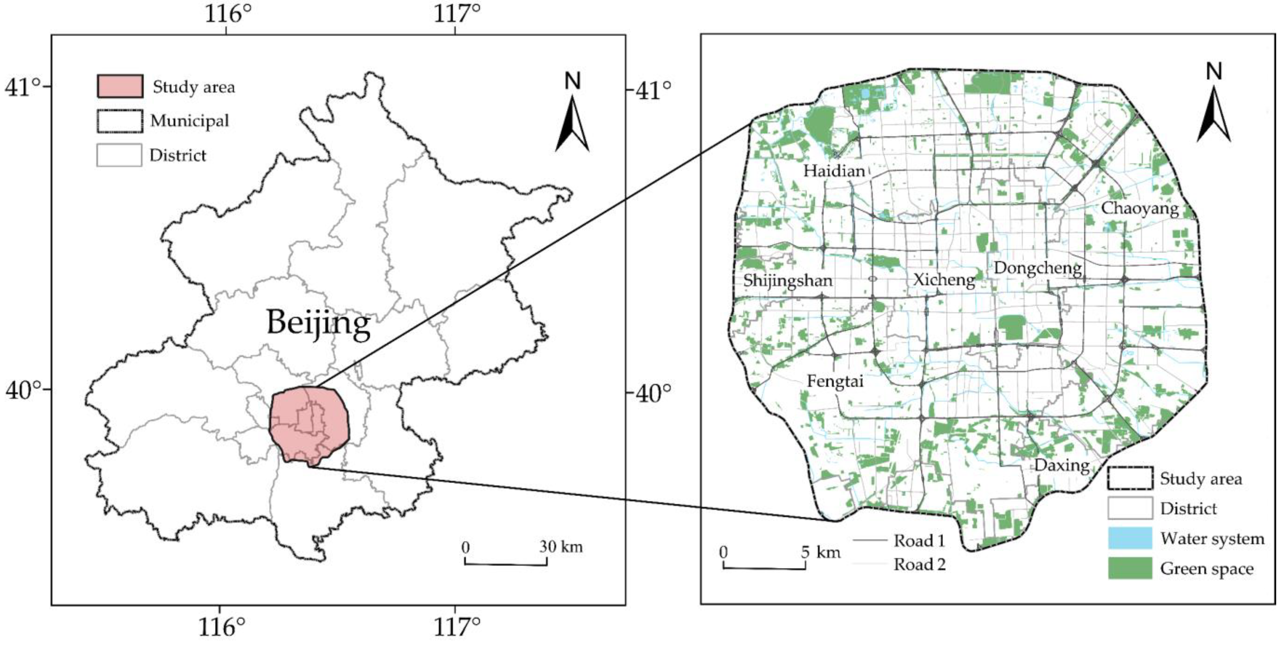
Beijing, the capital of China, is located in the north of China and comprises 16 districts under its jurisdiction, covering a total area of 16,410.54 square kilometers. The Fifth Ring Road, also known as “Wuhuanlu” in Chinese, is a highway encircling Beijing’s urban and suburban areas, serving as a boundary between them. As shown in Figure 1, the study area is within Beijing’s Fifth Ring Road (116°12′–116°32′ E, 39°45′–40°1′ N) with a total area of roughly 660 square kilometers. It includes the entirety of Xicheng and Dongcheng districts, the majority of Haidian, Chaoyang, Fengtai, Shijingshan districts, and a small portion of the northern region of Daxing district. The study area is the central urban area of Beijing, and it is marked by a favorable geographical position, adequate supporting facilities and a high population density. This area is a typical and important region for the growth of urban commercial formats, ranging from various formats such as catering, shopping, entertainment and others. The catering industry, in particular, is highly developed in this region, and it is characterized by a sizeable market scale, diverse operating modes, typical features, and representativeness.

The POI data used in this study are obtained from Amap (https://www.amap.com (accessed on 30 December 2021)) as of December 2021. After data cleaning and area selection, the core dataset required for this study was obtained. The research object dataset chosen from the selected datasets includes:

(1)

[cp], with a total of 92,668 catering points.

Based on prior knowledge, the candidate agglomeration kernel element datasets was selected to include:

(2)

[SC], with 210 shopping centers, which are comprehensive commercial complexes that house a large number of retail stores, dining establishments, entertainment facilities, and service amenities;

(3)

[SP], including 365 shopping plazas, 298 chain supermarkets, amounting to 663 points in total, which are generally smaller in scale and have a relatively focused commercial format, primarily focusing on retail and providing purchasing and sales services for goods;

(4)

[BS], including 6792 business office buildings, which are specifically designed and designated for housing offices and conducting business activities;

(5)

[RE], including 15,617 residential entry points, which are the designated locations through which individuals enter or exit residential areas or properties.

The datasets (2)~(5) are referred to as [Candidate] in this paper.

3. Overall Characteristics of the Density Distribution of Catering Points

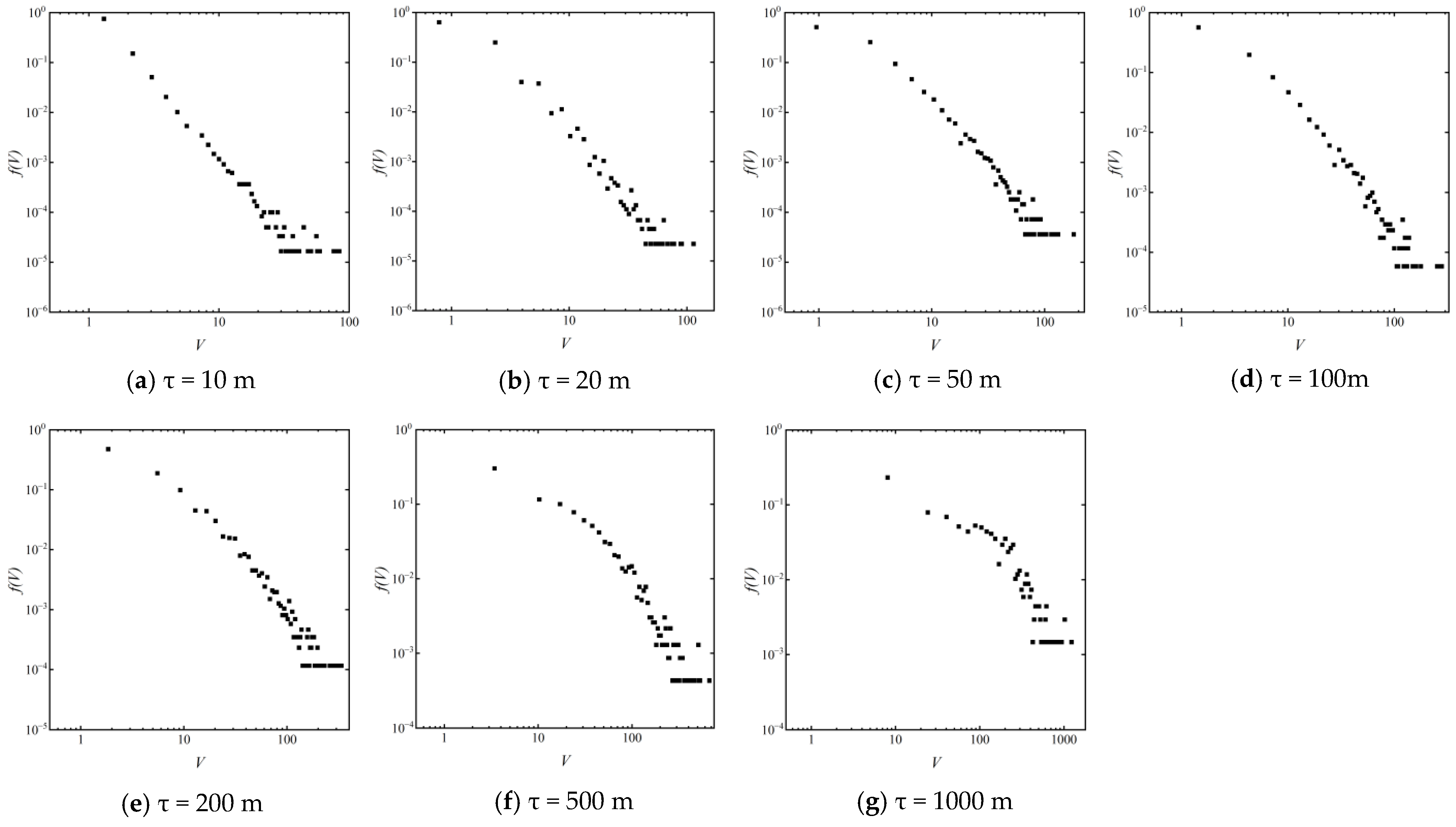
How to characterize the aggregation characteristics of catering points at a small scale? A commonly used and intuitive method is to characterize them with quantitative indicators of spatial density, such as a kernel density map. One advantage is that the spatial distribution of density is immediately apparent, while a disadvantage is that it fails to accurately capture the structural characteristics of density, posing challenges in forming a concise and precise description of the overall characteristics of catering points. Building upon this, the objective of this article is to establish a probability distribution of catering points density at a small scale. By doing so, a mathematical description of density distribution can be achieved. In this regard, the study area is divided into square grid cells, with candidate grid sizes of 10 m, 20 m, 50 m, 100 m, 200 m, 500 m, and 1000 m.

The statistical process is as follows: Let the scale be τ (such as 100 m).

(1)

Divide the study area into square grid cells with a side length of τ. The number of catering points in each grid cell is counted to obtain a set of grid cells containing more than 0 catering points, represented as $G=\left\{G_i\right|i=0,1,2,\dots \mathrm{n}\}$, where n is the total sample size. The number of catering points contained in $G_i$ is denoted as $N_i$, which represents the sample value of $G_i$.

(2)

Group the samples into a reduced number of “bins” using the data binning method, where each “bin” represents a specific interval of sample values. Set the number of bins as $m=100$. For comparability purposes, the same number of bins is used across all scales (corresponding to different τ, with different sample maximum and minimum values and bin widths). All samples are binned, and a value of $v_j\mathrm{corresponds}\mathrm{to}\mathrm{bin}{B}_j$, which is the central value of bin $B_j$. Since the planar area of all grids is the same, $v_j$ represents the number of catering points instead of density. The number of samples falling into bin $B_j$ is $s_j$. Using the method of frequency instead of probability, the probability distribution function is defined as:

$$f\left(V=v_j\right)=\frac{s_j}{n}, j=1,2,\dots m$$

(1)

The statistical parameters for each scale are shown in

Table 1. The statistical parameters for each scale.

Scale	Sample Size	Minimum	Maximum	Number of Bins	Information Entropy
10 m	60,271	1	84	100	1.301
20 m	45,561	1	114	100	1.577
50 m	27,755	1	181	100	2.166
100 m	17,206	1	278	100	2.168
200 m	8687	1	338	100	2.711
500 m	2322	1	672	100	3.799
1000 m	682	1	1228	100	4.345

.

3.1. Power-Law Distribution Characteristics of Planar Density

Statistical analysis reveals that at varying scales, the density of catering points exhibits power-law distribution characteristics to different degrees (Figure 2). Additionally, as the scale decreases, the power-law distribution characteristics become more noticeable. These findings suggest that (1) there is a prevalent competition among individual catering points for site selection, which is evidenced by their preferential attachment of individual catering points to other spatial entities (this topic will be discussed later in this article); (2) the site selection competition mechanism is more pronounced at smaller scales, revealing that catering points prioritize the “proximity” of smaller scales, such as “being 20 m closer to a shopping mall”, rather than whether they are in this block or another.

3.2. Information Entropy of Density Distribution

Information entropy reflects the level of uncertainty of a probability distribution, with higher values indicating more uniform probability distributions. Thus, to assess the uniformity of the density distribution of catering points across various scales, the information entropy is calculated (Table 1) using the following formula:

$$H\left(f\left(V\right)\right)={\sum }_{j=1}^{m}f\left(v_j\right){\log }_{2}f\left(v_j\right)$$

(2)

As shown in Table 1, the information entropy of the density distribution of catering points increases as the scale τ increases, indicating that within the range of 10~1000 m, the density distribution of catering points becomes increasingly non-uniform as the scale decreases. This observation reveals, from another perspective, the scale mechanism of site selection competition among individual catering points.

3.3. Mechanism of Preferential Attachment

Power-law distribution is perceived by researchers as a product of competition or preferential attachment mechanism [17] that is frequently observed in nature and human society. This study suggests that one significant contributing factor to the power-law distribution of the density of catering points at smaller scales is the distance-based preferential attachment mechanism in site selection competition; i.e., closer ones are preferred to attach. In addition, the agglomeration kernel elements are the objects that are “prioritized for attachment” by the catering points. This mechanism significantly impacts the aggregating of catering points, ultimately affecting the probability distribution characteristics of the density of catering points.

4. Aggregation Effect Analysis of Agglomeration Kernel Elements and Catering Points

Although individual analysis is still necessary, this paper aims to study the effect of a category of agglomeration kernel elements on the aggregation of catering points rather than focusing on individual or partial entities. This impact has the nature of categorical and represents the collection of all entities in this category. On this basis, comparisons are made between different categories. The purpose of this section is to establish a method for analyzing the aggregation effect and to conduct a categorization analysis of potential impacts by applying this method.

The research question of this section is abstracted as follows: given two finite sets of points, A and B, within the plane region r, then how to analyze the aggregation effect of A and B? The abstraction can simplify the solution process, as it operates solely on spatial position data. By inputting the [Candidate] as A and [cp] as B, the model can provide the solution of the problem. The primary approach for constructing the model involves establishing a spatial process, using distance as the independent variable, constructing a process function based on this, and analyzing the aggregation effect of A and B through process analysis.

4.1. Basic Spatial Process Function

Definition 1.

Distance–Quantity Function. Let $A=\left\{A_i,i=1,2,\dots n\right\}$ and $B=\left\{B_j,j=1,2,\dots m\right\}$ be two finite sets of points in a planar region r. Let $d_{i,j}$ be the distance between $A_i$ and $B_j$, whereas let $d_{j,i}$ be the distance between $B_j$ and $A_i$. $d_{i,B}$ denotes the minimum distance between $A_i$ and all points in B, which is referred to as the distance between $A_i$ and B. Its formula is given by:

$$d_{i,B}=Min\left(d_{i,1},d_{i,2},\dots ,d_{i,m}\right),$$

(3)

similarly,

$$d_{j,A}=Min\left(d_{j,1},d_{j,2},\dots ,d_{j,n}\right).$$

(4)

Let:

$$d_{max}=Max\left\{d_{i,B},d_{j,A};i=1,2,\dots n;j=1,2,\dots m\right\},$$

(5)

suppose a positive distance value, where  $0<x\le d_{max}$, and consider set A. Let  $N_{A\to B}\left(x\right)$ signify the count of points in A, whose minimum distance to a point in B is less than or equal to x:

$$N_{A\to B}\left(x\right)=\left|\left\{A_k|d_{k,B}\le x\right\}\right|$$

(6)

$N_{A\to B}\left(x\right)$ is referred to as the distance–quantity function by A to B. Similarly, the distance–quantity function by B to A is denoted by $N_{B\to A}\left(x\right)$.

4.2. Distance–Proportion Function

Definition 2.

Distance–Proportion (D-P) Function. Let $P_{A\to B}\left(x\right)$ be the distance–proportion function of A to B:

$$P_{A\to B}\left(x\right)=\frac{N_{A\to B}\left(x\right)}{n},0<x\le d_{max}$$

(7)

The D-P function reflects the proportion of A to B at varying distances, describing the two dimensions of “distance” and “proportion” of the “closeness” between A to B. The smaller the distance, the larger the proportion, indicating that A is “closer” to B.

Let $E\left(P_{A\to B},(x_s,x_t]\right)$ represent the average value of $P_{A\to B}\left(x\right)$ on the interval $(x_s,x_t]$ (i.e., the average proportion), which is expressed as:

$$E\left(P_{A\to B},(x_s,x_t]\right)=\frac{{\int }_{x_s}^{x_t}{P}_{A\to B}\left(x\right)dx}{x_t-x_s}$$

(8)

In particular, when $x_s=0$, the formula above can be represented as $E\left(P_{A\to B},x_t\right)$. For instance, $E\left(P_{A\to B},500 \mathrm{m}\right)$ represents the average proportion of A to B within 0–500 m.

4.3. Baseline Distribution and Baseline D-P function

While the D-P function reflects the degree of “closeness” between A and B, it does not account for the degree to which A actively approaches or moves away from B, given that it may be influenced by external factors. Thus, we define the “baseline spatial distribution”.

Definition 3.

Baseline Distribution. To investigate whether there is an effect of “approaching” or “moving away” by A to B based on distance, an ideal spatial distribution state is established for A, which is uniformly distributed within the region r, and this is referred to as the baseline distribution. It is assumed that under the baseline distribution, there is no effect of either “approaching” or “moving away” by A to B.

The D-P function of A to B under the baseline distribution is called the baseline D-P function, which is denoted as $P_{A\to B}^d\left(x\right)$. To define $P_{A\to B}^d\left(x\right)$, we use the D-P function of an infinite point set in the region r (represented by r) to B, thus:

$$P_{A\to B}^d\left(x\right)=P_{r\to B}\left(x\right)$$

(9)

It can be seen that $P_{r\to B}\left(x\right)$ is only related to r and B, and it is independent of A. However, since r is an infinite point set, it is difficult to obtain its analytical solution, so a simulation method is used to determine the numerical solution of $P_{r\to B}\left(x\right)$.

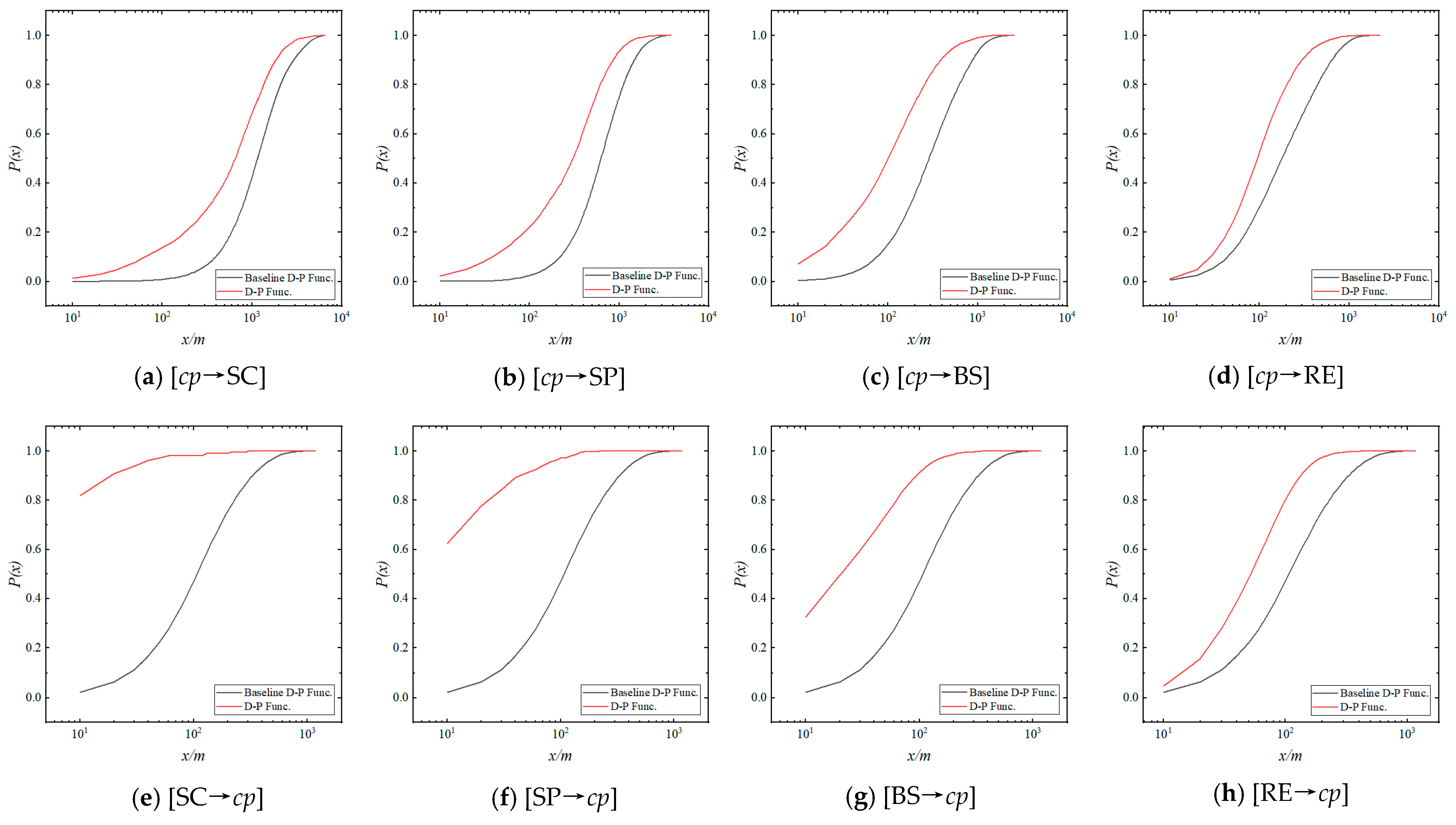
The definition of D-P function and baseline distribution provides a way to analyze the mutual effect of “approaching” between A and B. Accordingly, the D-P function and baseline D-P function between [Candidate] and [cp] are calculated, and their function graphs are shown in Figure 3. To highlight the comparison within smaller distances, a logarithmic transformation is applied to distance.

To quantitatively characterize the degree of the effect of “approaching” or “moving away” by A to B at different distances, the following function is defined.

Definition 4.

Distance–Proportion Coefficient Function. Let $P_{A\to B}\left(x\right)$ be the D-P function of A to B, and let $P_{A\to B}^d\left(x\right)=P_{r\to B}\left(x\right)$ be the baseline D-P function. Given a distance x, the distance–proportion coefficient function of A to B is defined as:

$$P_{A\to B}^c\left(x\right)=\frac{E\left(P_{A\to B},\hspace{1em}x\right)}{E\left(P_{A\to B}^d, x\right)},0<x\le d_{max}$$

(10)

If $P_{A\to B}^c\left(x\right)>1$, A is considered “approaching” B at the scale of x, if $P_{A\to B}^c\left(x\right)<1$, A is considered “moving away” from B at the scale of x. When $x=d_{max}$, it is considered at the global scale.

Definition 5.

Aggregation Effect. Given a distance x, if $P_{A\to B}^c\left(x\right)>1$ and $P_{B\to A}^c\left(x\right)>1$, A and B are considered to exhibit an aggregation effect at the scale x (i.e., both are “approaching” each other). In particular, if $P_{A\to B}^c\left(d_{max}\right)>1$ and $P_{B\to A}^c\left(d_{max}\right)>1$, A and B are considered to exhibit an aggregation effect at the global scale.

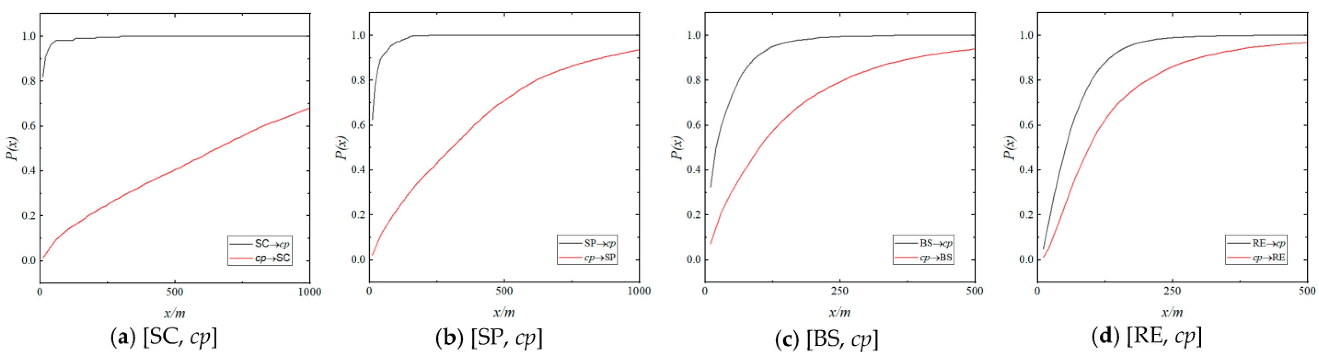
In Figure 3, the D-P function curves of [cp→Candidate] and [Candidate→cp] are located above their respective baseline D-P function curves, indicating that the [Candidate] and [cp] are “approaching” each other across all scales from 0 to ${\mathrm{d}}_{\mathrm{m}ax}$, implying an aggregation effect at all scales from 0 to ${\mathrm{d}}_{\mathrm{m}ax}$. Moreover, the smaller the scale, the higher the degree of aggregation (i.e., the higher the proportion compared to the baseline distribution).

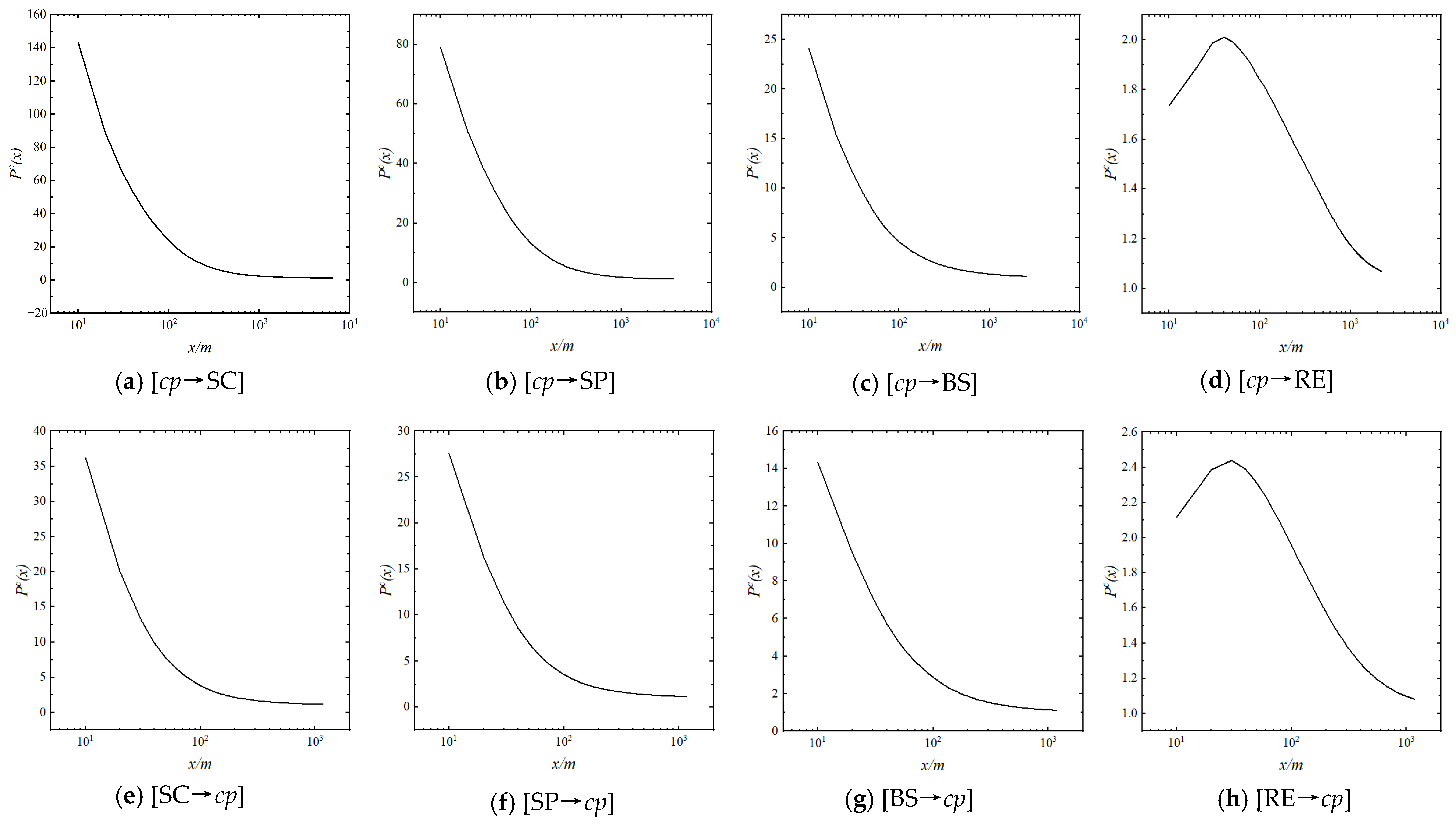
Figure 4 illustrates the distance–proportion coefficient function curves (with a log distance) for [cp→Candidate] and [Candidate→cp]. It can be observed that the proportion coefficient rapidly diminishes at small distances and then gradually flattens out. This provides the foundation for analyzing the aggregation effect at small scales in particular and establishes preconditions to investigate the agglomeration effect further.

Table 2. Proportion Coefficient at Some Scales.

	Pc(x)
	100 m	200 m	500 m	dmax
[cp→SC]	23.908	11.379	4.302	1.116
[cp→SP]	13.343	6.702	2.804	1.120
[cp→BS]	4.628	2.859	1.731	1.106
[cp→RE]	1.841	1.639	1.356	1.069
[SC→cp]	3.844	2.166	1.372	1.134
[SP→cp]	3.561	2.091	1.354	1.128
[BS→cp]	2.878	1.875	1.299	1.108
[RE→cp]	1.957	1.574	1.222	1.081

lists the proportion coefficient values at some small scales of [cp→Candidate] and [Candidate→cp].

4.4. Symmetry Analysis of Aggregation Effect

The proportion coefficient reflects the degree of unilateral participation of a point set in the aggregation effect. The symmetry of two sets of D-P functions is analyzed by comparison. To that end, the following function is defined.

Definition 6.

Distance–Proportion Symmetric Coefficient Function. The distance–proportion symmetric coefficient function for A and B is given as:

$$P_{A,B}^s\left(x\right)=1-\frac{\left|E\left(P_{A\to B},x\right)-E\left(P_{B\to A},x\right)\right|}{E\left(P_{A\to B},x\right)+E\left(P_{B\to A},x\right)}, 0<x\le d_{max}$$

(11)

Figure 5 shows all D-P function curves for [Candidate, cp]. The [Candidate→cp] D-P function curves are all located above the [cp→Candidate] D-P function curves, which indicates that all [Candidate] have a greater proportion of participation in the aggregation effect at all scales. This demonstrates that [cp] are not exclusively connected to a single [Candidate] but display an aggregation effect with all [Candidate].

Table 3. Proportion Symmetric Coefficients of [Candidate, cp].

	Ps(x)
	100 m	200 m	500 m
[SC, cp]	0.159	0.239	0.396
[SP, cp]	0.260	0.381	0.604
[BS, cp]	0.610	0.724	0.865
[RE, cp]	0.712	0.815	0.917

lists the symmetric coefficients at some small scales.

5. Agglomeration Effect Analysis of Agglomeration Kernel Elements to Catering Points

Definition 7.

Agglomeration Effect. If A and B exhibit aggregation effects at scale x, and $\left|A\right|\ll \left|B\right|$ (i.e., asymmetric in sample size), then there is an effect of agglomeration by A to B at scale x.

Based on this definition and the results in Section 4.3, it can be inferred that all [Candidate→cp] display agglomeration effects at scales ranging from 0 to $d_{max}$.

5.1. Basic Characteristic Parameters

Definition 8.

Distance–Agglomeration Proportion Function. The distance–agglomeration proportion function by A to B is given as:

$$C_{A\to B}^p\left(x\right)=P_{B\to A}\left(x\right)=\frac{N_{B\to A}\left(x\right)}{m},\hspace{1em}0<x\le d_{max}$$

(12)

It reflects the proportion of the agglomeration effect by A to B at scale x. The value of the function $C_{A\to B}^p\left(x\right)$ is identical to that of the D-P function $P_{B\to A}\left(x\right)$ by B to A.

Definition 9.

Distance–Agglomeration Ratio Function. The distance–agglomeration ratio function by A to B is given as:

$$C_{A\to B}^r\left(x\right)=\frac{N_{B\to A}\left(x\right)}{N_{A\to B}\left(x\right)},\hspace{1em}0<x\le d_{max},$$

(13)

i.e., it refers to the number of points in B that correspond to each point in A at scale x, which reflects the agglomeration effect in terms of quantity.

Table 4. Agglomeration Effect Basic Parameters of [Candidate→cp].

	Cp (x)			Cr (x)
	100 m	200 m	500 m	100 m	200 m	500 m
[SC→cp]	0.138	0.217	0.406	61.757	96.332	178.329
[SP→cp]	0.222	0.371	0.712	31.710	51.730	99.089
[BS→cp]	0.499	0.729	0.941	7.427	10.031	12.789
[RE→cp]	0.522	0.796	0.969	3.873	4.853	5.758

lists the agglomeration effect basic parameters of [Candidate→cp] at some small scales.

5.2. Distance–Density Function

Definition 10.

Distance–Area Function. Within the planar region r, there is a finite set of points $A=\left\{A_i,i=1,2,\dots n\right\}$. Let $R_{A_i}\left(x\right)$ denote the buffer region with center A_i and distance x. Let $R_A\left(x\right)=[R_{A_1}\left(x\right)\cup R_{A_2}\left(x\right)\cup \dots \cup R_{A_n}\left(x\right)]\cap r$, which is the union of all buffer regions within r. $R_A\left(x\right)$ is referred to as the buffer region with distance x of A. Let $Are{a}_A\left(x\right)$ be the area of $R_A\left(x\right)$, which is known as the distance–area function of A. Utilizing spatial analysis methods, $Are{a}_A\left(x\right)$ can be calculated.

Definition 11.

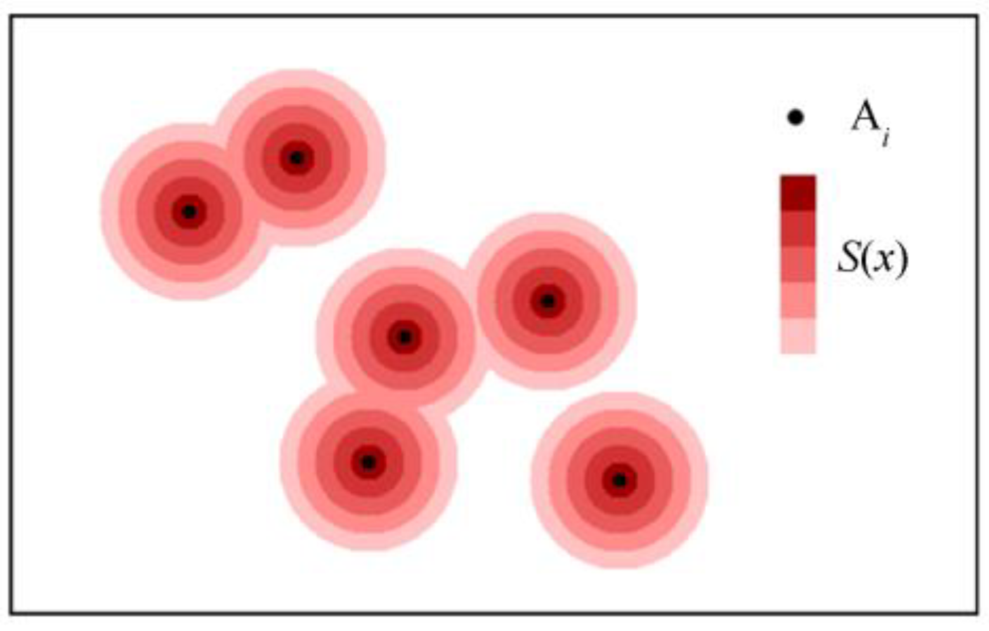
Distance–Density (D-S) Function. Given a distance x, adding a small distance increment ∆x, then the distance–density function by A to B is as follows:

$$S_{A\to B}\left(x\right)=\underset{\Delta x\to 0}{\lim }\frac{N_{B\to A}\left(x,\Delta x\right)}{Are{a}_A\left(x+\Delta x\right)-Are{a}_A\left(x\right)},\hspace{1em}0<x\le d_{max},$$

(14)

where

$$N_{B\to A}\left(x,\Delta x\right)=\left|\left\{B_k|x<d_{k,A}\le x+\Delta x\right\}\right|$$

(15)

After increasing a small distance increment $\Delta x$, the buffering area of A expands by a small amount $Are{a}_A\left(x+\Delta x\right)-Are{a}_A\left(x\right)$, and the D-S function reflects the average density of points in B located within this small area (Figure 6). As $\Delta x\to 0$, $S_{A\to B}\left(x\right)$ represents the density at the boundary of the buffering area with a distance of x. The D-S function characterizes the impact of agglomeration effect on density.

Definition 12.

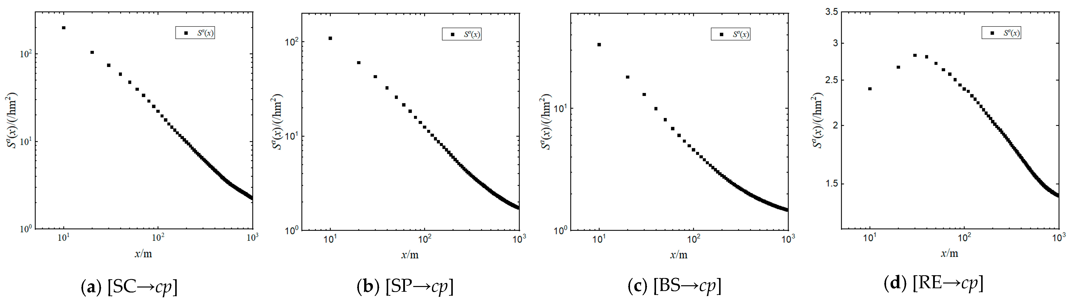
Distance–Average Density (D-S^a) Function. The distance–average density function by A to B is as follows:

$$S_{A\to B}^a\left(x\right)=\frac{N_{B\to A}\left(x\right)}{Are{a}_A\left(x\right)},0<x\le d_{max}$$

(16)

The definition implies that $S_{A\to B}^a\left(x\right)$ describes the average density of B within the buffering area $R_A\left(x\right)$ of A.

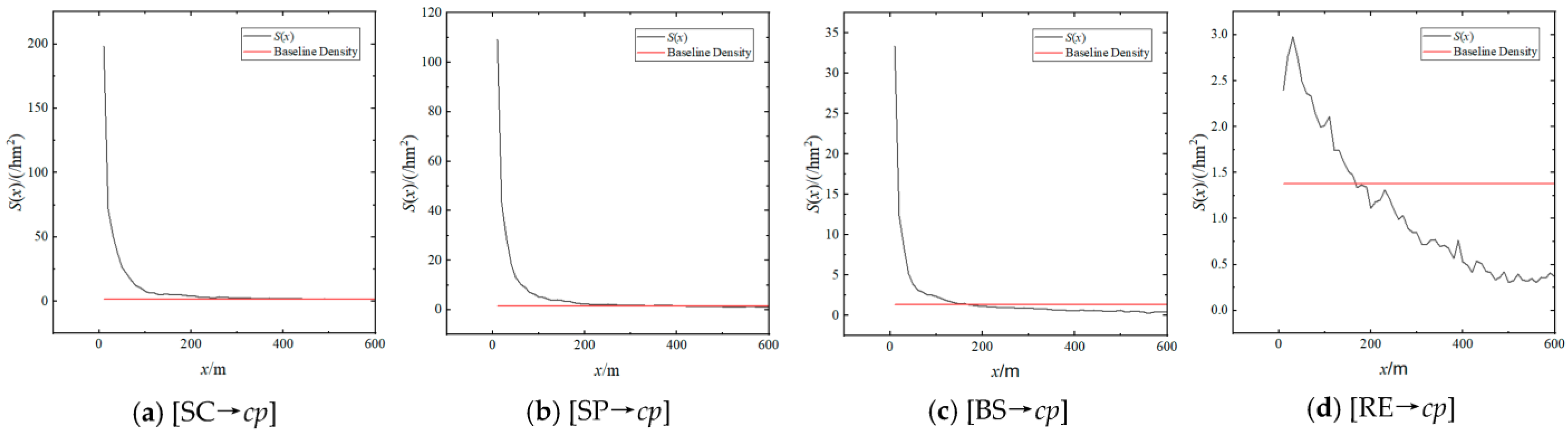
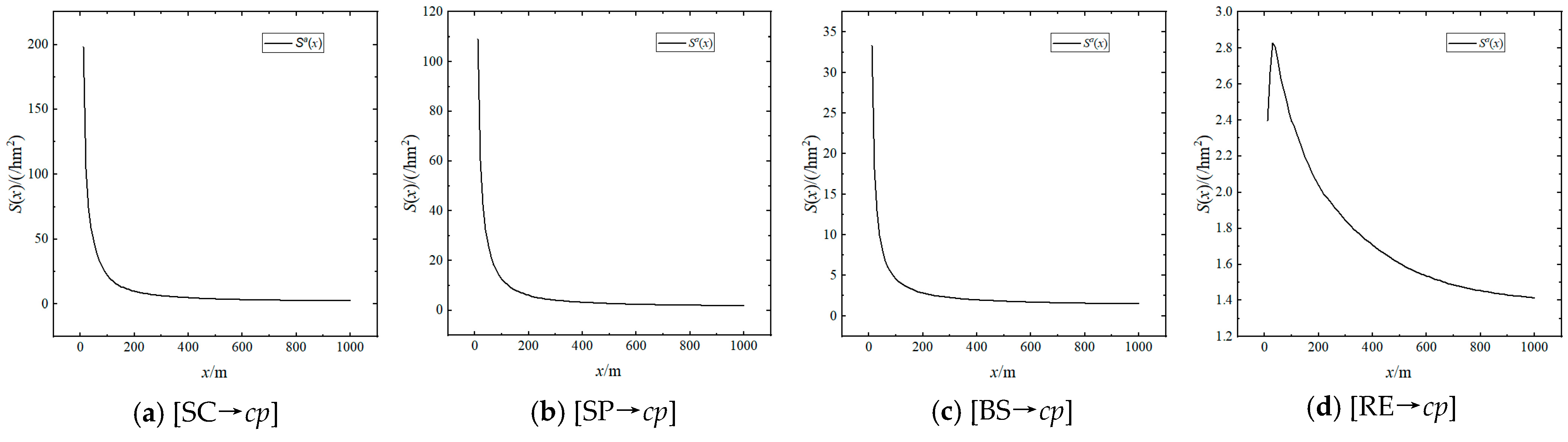
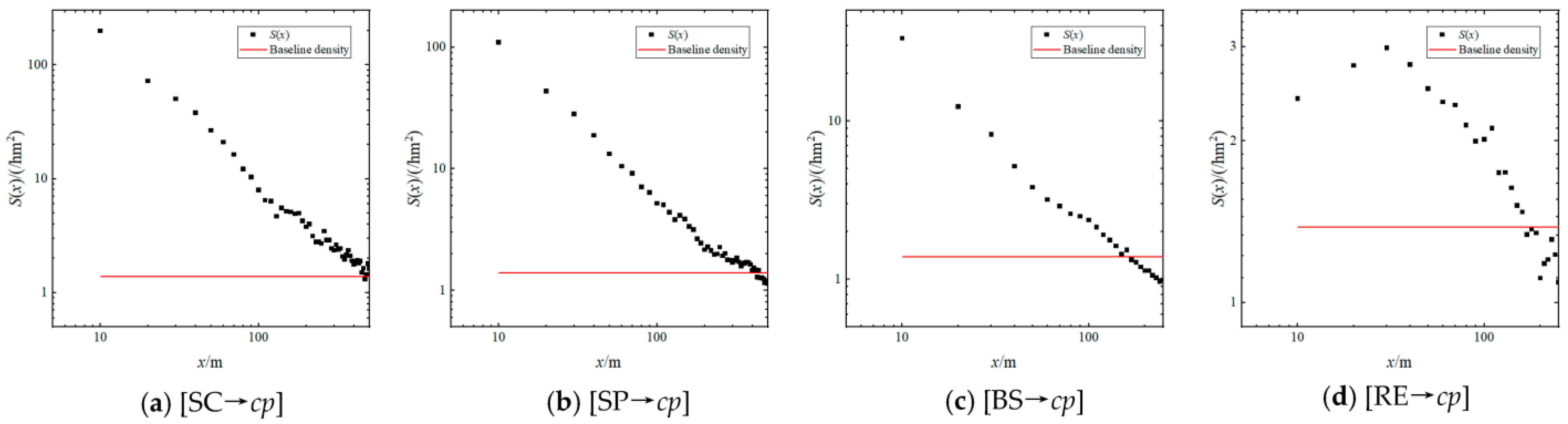
Figure 7 and Figure 8 shows the function curves of $S\left(x\right)$ and $S^a\left(x\right)$ of [Candidate→cp], respectively. It is evident that both functions show a rapid decrease within 200 m and then become stable.

Definition 13.

Baseline Density and Cutoff-Distance. The density of B under the baseline distribution is referred to as the baseline density of B. The distance x at which $S_{A\to B}\left(x\right)$ first decays to baseline density is called the cutoff distance by A to B. Statistical analysis shows that the baseline density of catering points in the study area is 1.382/hm².

Table 5. Density Analysis Parameters of [Candidate→cp].

	S(x)(/hm2)			Sa(x)(/hm2)			Cutoff- Distance(m)
	100 m	200 m	500 m	100 m	200 m	500 m
[SC→cp]	7.965	3.769	1.630	22.116	9.856	3.727	800
[SP→cp]	5.172	2.152	1.131	12.468	5.973	2.618	450
[BS→cp]	2.365	1.133	0.615	4.580	2.827	1.801	170
[RE→cp]	2.012	1.109	0.307	2.394	2.038	1.606	150

lists the density analysis parameters of [Candidate→cp].

5.3. Distance–Density Correlation

In this section, correlation analysis is conducted between distance and density. Through curve fitting, it is found that at small scales, the D-S functions and D-S^a functions of [Candidate→cp] exhibit good power-law relationships (Figure 9 and Figure 10). Taking [SC→cp] as an example, a power-law distribution was fitted with parameters a = 3905.2888 and b = −1.298, resulting in an R² value of 0.9966. This indicates a power-law decay of density as distance increases, which can be expressed as:

$$S\left(x\right)~x^{-\beta }$$

(17)

$$S^a\left(x\right)~x^{-{\beta }_a}$$

(18)

The power-law decay relationship between density and distance provides a mathematical method for accurately describing the agglomeration effect by agglomeration kernel elements to catering points as well as a more precise basis for the mechanism of preferential attachment in the competition for catering point site selection.

5.4. Effective Distance of Agglomeration Effect

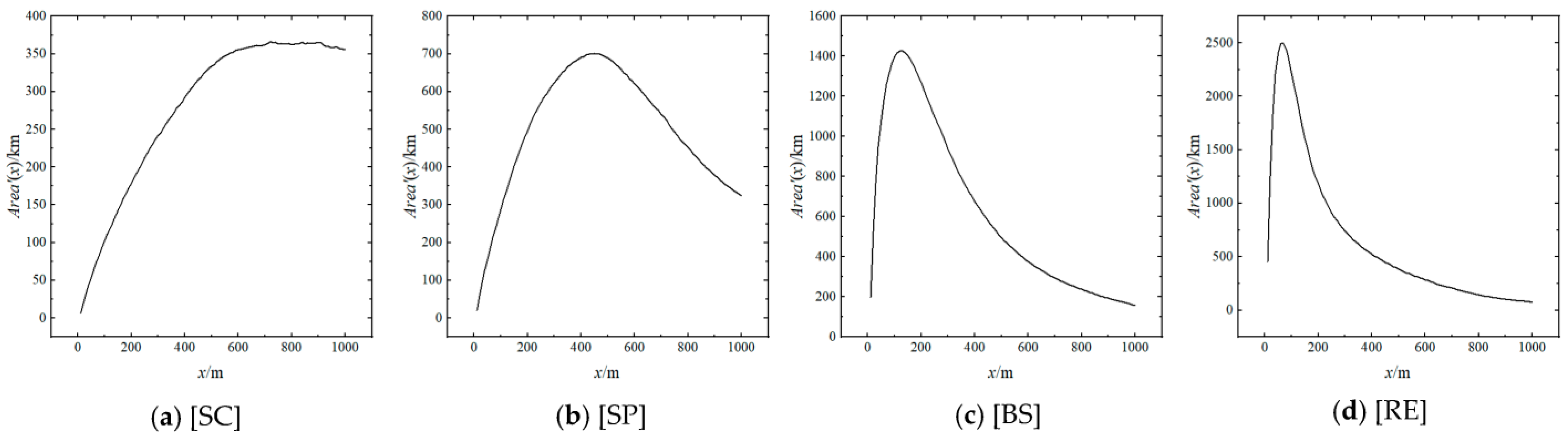
Looking back, let us analyze the derivative of the distance–area function, which represents the relationship between the corresponding growth rate in buffering area and x with a small distance increment $\Delta x$. It is defined as:

$${Area}_A^{\prime }\left(x\right)=\underset{\Delta x\to 0}{\lim }\frac{Are{a}_A\left(x+\Delta x\right)-Are{a}_A\left(x\right)}{\Delta x}$$

(19)

Figure 11 illustrates the ${Area}^{\prime }\left(x\right)$ function curves of [Candidate].

Figure 11 illustrates the presence of an extremum point on each curve. The x-axis value corresponding to the extremum point is referred to as the “inflection point distance”, which represents a change in the area growth rate. The inflection point distance is dependent on the size and spatial location of the [Candidate]. In Figure 11, when x is small, each $R_{A_i}\left(x\right)$ in A does not intersect the others. At this point, the relationship between ${Area}_A^{\prime }\left(x\right)$ and x is roughly proportional (as evidenced by the linear relationship of each curve before the inflection point in Figure 11, which is analogous to the derivative of the area of a circle that is proportional to the radius). As x increases, each $R_{A_i}\left(x\right)$ begins to intersect the others, the intersecting area becomes larger, and the contribution of more $R_{A_i}\left(x\right)$ to ${Area}_A^{\prime }\left(x\right)$ decreases until it disappears. Therefore, ${Area}_A^{\prime }\left(x\right)$ has an inflection point, and the value decreases after the inflection point.

This paper suggests that using the “inflection point distance” to represent the effective agglomeration distance of A is appropriate. Notably, the “inflection point distance” does not indicate the agglomeration distance of an individual in A but rather serves as a representation of the effective agglomeration distance of A as a whole. This is because after the inflection point, the density of ${Area}_A^{\prime }\left(x\right)$ no longer represent the total agglomeration effect by A. The excellent correspondence between the inflection point distance and the cutoff distance (as shown in Table 5) provides strong support for the use of the inflection point distance to represent the effective agglomeration distance of A.

5.5. Explanation of The Power-Law Distribution Characteristic of Catering Points Density

Let [Candidate] be A, [cp] be B, and the inflection point distance be $d_c$. $S_{A\to B}\left(x\right)$ is the D-S function by A to B. Based on Equation (17), assume:

$$S_{A\to B}\left(x\right)=a{x}^{-\beta },\hspace{1em}0<x\le d_c$$

(20)

Base on the analysis in Section 5.4, let us assume that the following equation holds true (i.e., the new area is proportional to the distance before the inflection point):

$${Area}_A^{\prime }\left(x\right)=bx,\hspace{1em}0<x\le d_c,$$

(21)

then,

$$Are{a}_A\left(d_c\right)={\int }_0^{d_c}{Area}_A^{\prime }\left(x\right)dx=\frac{b{d}_c{}^2}{2}.$$

(22)

Let

$$s=S_{A\to B}\left(x\right)=a{x}^{-\beta },\hspace{1em}0<x\le d_c,$$

(23)

and let $P\left(s\right)$ denote the probability density; then, it can be deduced that:

$$P\left(s\right)=\frac{{Area}_A^{\prime }\left(x\right)}{Are{a}_A\left(d_c\right)}=\frac{2x}{d_c^2}=\frac{2a^{\frac{1}{\beta }}}{d_c^2}{s}^{-\frac{1}{\beta }}.$$

(24)

Let $\mathsf{\gamma }=\frac{1}{\beta }$; then,

$$P\left(s\right)\propto s^{-\gamma },$$

(25)

i.e., the density distribution of B within $R_A\left(d_c\right)$ of A follows a power-law distribution. The density distribution within the study area is a result of the compounding effect of various agglomeration kernel elements. In addition, the varying inflection point distances of each [Candidate] result in a more pronounced power-law characteristic of the catering points density distribution at smaller scales, which is particularly significant at scales below 200 m.

6. Conclusions

Based on POI data, this study conducted statistical analysis on small-scale aggregation characteristics of urban catering points, and we concluded that the agglomeration kernel elements are important elements influencing the aggregation of catering points. A corresponding analysis model was proposed, and the impact analysis of candidate points sets was carried out from two aspects: aggregation effect and agglomeration effect. The following conclusions were drawn:

(1)

The spatial density distribution of catering points in the study area presents power-law distribution characteristics at scales ranging from 10 to 1000 m, with a more pronounced characteristic at smaller scales. This data-driven finding interprets the mechanism of preferential attachment in the competition for catering point site selection.

(2)

Using the spatial process analysis method, an aggregation effect analysis model based on the distance–proportion function and an agglomeration effect analysis model based on the distance–density function were established. An empirical analysis between the candidate points sets and the catering points set was conducted, which demonstrated the validity of the model.

(3)

The aggregation effect analysis revealed that the candidate agglomeration kernel elements exhibited a global-scale aggregation effect on catering points, indicating their categorical impact on the aggregation characteristics of catering points.

(4)

The agglomeration effect analysis revealed that the candidate agglomeration kernel elements exhibit an agglomeration effect on catering points. Two important conclusions were drawn: firstly, there is a power-law decay relationship between the density and distance of catering points, revealing the mechanism of preferential attachment in the competition for catering point site selection. Secondly, it identified the effective distance of agglomeration effect by different agglomeration kernel elements.

(5)

Based on the conclusions derived from the agglomeration effect analysis, mathematical methods were utilized to explain the power-law distribution characteristics of density of catering points. The study formed an organic connection between micro-level effect analysis and macro-level characteristic analysis.

The analysis model proposed in this study also provides a reference for analyzing the aggregation characteristics and influencing elements of other urban commercial formats.

References

- Hotelling, H. Stability in Competition. Econ. J. 1929, 39, 41–57. [Google Scholar] [CrossRef]
- Oppewal, H.; Holyoake, B. Bundling and retail agglomeration effects on shopping behavior. J. Retail. Consum. Serv. 2004, 11, 61–74. [Google Scholar] [CrossRef]
- James, P.; Bound, D. Urban morphology types and open space distribution in urban core areas. Urban Ecosyst. 2009, 12, 417–424. [Google Scholar] [CrossRef]
- Yang, Z.; Sliuzas, R.; Cai, J.; Ottens, H.F. Exploring spatial evolution of economic clusters: A case study of Beijing. Int. J. Appl. Earth Obs. Geoinf. 2012, 19, 252–265. [Google Scholar] [CrossRef]
- Lan, T.; Yu, M.; Xu, Z.; Wu, Y. Temporal and spatial variation characteristics of catering facilities based on POI data: A case study within 5th ring road in Beijing. Procedia Comput. Sci. 2018, 131, 1260–1268. [Google Scholar] [CrossRef]
- Li, Y.; Liu, H.; Wang, L.-E. Spatial distribution pattern of the catering industry in a tourist city: Taking Lhasa city as a case. J. Resour. Ecol. 2020, 11, 191–205. [Google Scholar]
- Prayag, G.; Landré, M.; Ryan, C. Restaurant location in Hamilton, New Zealand: Clustering patterns from 1996 to 2008. Int. J. Contemp. Hosp. Manag. 2012, 24, 430–450. [Google Scholar] [CrossRef]
- Wang, T.; Wang, Y.; Zhao, X.; Fu, X. Spatial distribution pattern of the customer count and satisfaction of commercial facilities based on social network review data in Beijing, China. Comput. Environ. Urban Syst. 2018, 71, 88–97. [Google Scholar] [CrossRef]
- Wang, W.; Wang, S.; Chen, H.; Liu, L.; Fu, T.; Yang, Y. Analysis of the characteristics and spatial pattern of the catering industry in the four central cities of the Yangtze River Delta. ISPRS Int. J. Geo-Inf. 2022, 11, 321. [Google Scholar] [CrossRef]
- Zheng, D.; Li, C. Research on Spatial Pattern and Its Industrial Distribution of Commercial Space in Mianyang Based on POI Data. J. Data Anal. Inf. Process. 2020, 8, 20. [Google Scholar] [CrossRef] [Green Version]
- Fang, Y.; Mao, J.; Liu, Q.; Huang, J. Exploratory space data analysis of spatial patterns of large-scale retail commercial facilities: The case of Gulou District, Nanjing, China. Front. Archit. Res. 2021, 10, 17–32. [Google Scholar] [CrossRef]
- Reigadinha, T.; Godinho, P.; Dias, J. Portuguese food retailers–Exploring three classic theories of retail location. J. Retail. Consum. Serv. 2017, 34, 102–116. [Google Scholar] [CrossRef] [Green Version]
- Zheng, T. Relationship between Urban Retail Commercial Space Distribution and the Road Network & Population Distribution: Comparison of Mobility and Non-Current Factors. IOSR J. Bus. Manag. 2019, 21, 42–48. [Google Scholar]
- Porta, S.; Strano, E.; Iacoviello, V.; Messora, R.; Latora, V.; Cardillo, A.; Wang, F.; Scellato, S. Street centrality and densities of retail and services in Bologna, Italy. Environ. Plan. B Plan. Des. 2009, 36, 450–465. [Google Scholar] [CrossRef] [Green Version]
- Saraiva, M.; Pinho, P. Spatial modelling of commercial spaces in medium-sized cities. GeoJournal 2017, 82, 433–454. [Google Scholar] [CrossRef]
- Wang, F.; Niu, F.-Q. Urban commercial spatial structure optimization in the metropolitan area of Beijing: A microscopic perspective. Sustainability 2019, 11, 1103. [Google Scholar] [CrossRef] [Green Version]
- Barabási, A.-L.; Albert, R. Emergence of scaling in random networks. Science 1999, 286, 509–512. [Google Scholar] [CrossRef] [PubMed] [Green Version]
Figure 1.
Map of the Fifth Ring Road of Beijing.
Figure 2.
The Power-Law Distribution Characteristics of Catering Points Density at Different Spatial Scales.
Figure 3.
D-P Functions and Baseline D-P Functions of [cp→Candidate] and [Candidate→cp].
Figure 4.
Distance–Proportion Coefficient Function of [cp→Candidate] and [Candidate→cp].
Figure 5.
D-P Function Curves of [Candidate, cp].
Figure 6.
The Schematic Diagram of D-S Function.
Figure 7.
D-S Function of [Candidate→cp].
Figure 8.
D-Sa Function of [Candidate→cp].
Figure 9.
Power-Law Characteristic of D-S Functions of [Candidate→cp].
Figure 10.
Power-Law Characteristic of D-Sa Functions of [Candidate→cp].
Figure 11.
Function Curves of [Candidate].