
Classification of Spatial Objects with the Use of Graph Neural Networks

1
Institute of Spatial Management, Wrocław University of Environmental and Life Sciences, 50-375 Wrocław, Poland
2
Institute of Geodesy and Geoinformatics, Wrocław University of Environmental and Life Sciences, 50-375 Wrocław, Poland
3
Wroclaw Institute of Spatial Information and Artificial Intelligence, 50-374 Wrocław, Poland
4
Institute of Automatic Control and Robotics, Poznan University of Technology, 60-965 Poznań, Poland
*
Author to whom correspondence should be addressed.
ISPRS Int. J. Geo-Inf. 2023, 12(3), 83; https://doi.org/10.3390/ijgi12030083
Submission received: 20 December 2022
/
Revised: 6 February 2023
/
Accepted: 18 February 2023
/
Published: 21 February 2023
Abstract
:Classification is one of the most-common machine learning tasks. In the field of GIS, deep-neural-network-based classification algorithms are mainly used in the field of remote sensing, for example for image classification. In the case of spatial data in the form of polygons or lines, the representation of the data in the form of a graph enables the use of graph neural networks (GNNs) to classify spatial objects, taking into account their topology. In this article, a method for multi-class classification of spatial objects using GNNs is proposed. The method was compared to two others that are based solely on text classification or text classification and an adjacency matrix. The use case for the developed method was the classification of planning zones in local spatial development plans. The experiments indicated that information about the topology of objects has a significant impact on improving the classification results using GNNs. It is also important to take into account different input parameters, such as the document length, the form of the training data representation, or the network architecture used, in order to optimize the model.
1. Introduction
The classification of spatial objects aims to assign a spatial object to the appropriate class from a given set of classes based on the values of the object’s attributes. These characteristics can be distance, direction, or topological relationships between spatial objects [1]. In geographic information systems (GISs), machine-learning-based classification algorithms are widely used in the field of remote sensing. Both supervised and unsupervised learning techniques are used for the classification of images such as aerial or satellite photos. Convolutional neural networks are particularly useful in such applications because they take into account the topology and neighborhood of pixels using masks in the learning process.
The use of machine learning algorithms for raster data yields very good results and is well described in the literature. However, for features represented in a vector model, the preparation of data for machine learning is more difficult. In that case, a graph structure is required to fully describe the topology, which cannot be projected onto a single vector. Spatial data, represented as polygons such as cadastral parcels or planning zones, can be represented as a graph where each node represents a spatial object (e.g., parcel) and edges represent the neighborhood of the spatial object (that is, the topology in GISs). GNNs are able to learn representations of each node by aggregating information from its neighboring nodes and edges. This allows them to capture the contextual information from the surrounding objects and improve the classification of the central object. In the field of spatial planning, it is important to take into account the dependencies between the functions of individual areas. This relationship results from the fact that the function of a given area is related to and often determined by the functions of neighboring areas. As a result, it is important to take this dependence into account when predicting the function of a specific area. In geographic information systems, this is a common problem that involves many land features that are dependent on their neighbors.
Text classification is one of the most-popular tasks in machine learning. It is essentially the process of assigning a given set of data (in this case, text documents) to one or more classes assuming a predefined set of classes. There are a number of methods for classifying documents, both supervised and unsupervised. These include algorithms such as support vector machine (SVM), the naive Bayes classifier, and XGBoost. More advanced methods include those that use large language models such as BERT and GPT-3.
The aim of this article is to develop a multi-class classification method for spatial objects (represented as polygons) using graph neural networks, which takes into account the textual description of the object and information about its geometry and mutual neighborhood (topology) with other objects. We chose spatial development plans as a case study. These are documents that consist of two integral parts: a graphical (plan drawing) and a descriptive (plan text) part. The graphical part represents spatial objects such as the boundary of the plan, planning zones, or other objects regulating land use, such as building lines, restricted use zones, conservation zones, etc. All spatial objects that appear on the plan drawing have a corresponding reference in the plan text. The basic reference unit in the plan is the planning zone, for which detailed provisions are formulated regulating the use of space in a given area. The basic information characterizing the planning zone is the category of future land use, such as residential development areas, communication areas, service areas, etc.
In the absence of a planning data model, as is the case in many European countries, such as Poland, the heterogeneity of planning data models is very high. In addition, the classifications of future land use are diverse. Currently, in the absence of a planning data model, as well as a standard for the classification of land uses applied to planning zones, there is still limited use of such data. It is not possible to integrate and comprehensively compare them on a larger scale, such as an entire region [2]. The developed method of classifying spatial objects using graph neural networks has been applied to spatial development plans. In this case, it aims to support the process of standardizing the future land use classification in plans and, thus, harmonizing them.
This article describes three methods for classifying planning zones based on fragments of text and information on the mutual neighborhood of spatial objects. Two of these methods are based on the use of the XGBoost classifier, while the third method uses graph neural network models. In order to find the best of these models, a series of experiments was conducted using the multilingual language model sentence embeddings to vectorize the text [3,4] and various graph neural network models. The aim of the experiments was to assign a specific future land use category to each planning zone.
The article is related to our previous work. In [2], we developed a model for classifying planning zones using supervised and unsupervised learning methods. We used a developed network architecture based on convolutional neural networks for this purpose. In the created classification model, the training data consisted of text data, i.e., fragments of text from plans. The model was trained on the basis of these data. However, in the present study, we also took into account the mutual spatial relationships of objects, i.e., the arrangement of planning zones with respect to each other in geographical space. The consideration of the spatial aspect was possible thanks to the use of graph neural networks. They allowed for the consideration of the topology and geometric characteristics of objects represented in the form of a graph.
2. Related Work
Deep learning has been successfully used for the analysis of raster data to detect geographical features or phenomena based on images [5,6,7,8]. It is common to use neural networks to detect buildings or other spatial objects in satellite images [9] or to classify land cover [10].
The graph as a mathematical structure is used to present and study the relationships between objects. The representation of data as graphs, along with the registration of relations between particular objects under consideration have been very popular in recent years. Among the most-obvious applications of graphs are molecule representation, transportation maps, social networks, citation networks, etc. The latter one, close to ours, is constructed as follows. The nodes of the graph are scientific articles; each article is assigned to one of the given categories; connections between articles (edges of the graph) are created on the basis of citations, while the properties of individual nodes are keywords that describe a given article.
Graph neural networks (GNNs) are a response to the need to process such mathematical structures as graphs. GNNs were introduced already in [11,12], but in recent years, numerous publications have shown a growing interest in this subject, both at the level of designing new structures of this type of neural network and their specific applications.
For example, the analysis of the molecule representations mentioned above led scientists to discover new antibiotics [13,14]. Another example is the work [15], which presented the prediction of the travel time solution used in Google Maps.
As a rule, graphs composed of nodes and their connecting edges do not contain information about the spatial distribution of individual vertices. In publications related to GISs, this is often the issue, where the GNNs are combined with, namely, the graph structure of the data together with the geographic spatial position of the nodes. In the literature, not only related to geographic data, it is possible to find solutions that address this issue. An example would be the Spatial GNNs presented in [16]. Another solution, based on positional encoder GNNs, was given in [17]. In the paper [18], a neighbor supporting graph convolutional neural network was used for urban scene classification, which consisted of visual and semantic features and exhibited spatial relationships among land use types. Other examples of GNN applications in GISs include, for example, traffic forecasting problems [19], road surface extraction from high-resolution remote sensing images [20], or site selection tasks [21].
One of the most-popular datasets is the CORA citation dataset [22], which is freely available, so there are plenty of examples of implementations using these data in the literature. In addition, the example we present is from the field of natural language processing (NLP); hence, the examples from the CORA set were easier for us to understand and then develop towards our needs.
There are now a number of Python packages that support GNNs. Among them, it is possible to find TensorFlow and Keras. However, there are a number of specialized TensorFlow-based libraries that provide rich GNN APIs, such as Spektral [23] or StellarGraph [24], while coding with TensorFlow might be rather low-level. Of course, the approaches may be different; first of all, GNNs can be used in two main ways:
- Classification of nodes, where one extended graph is sufficient for the analysis, in which we do not know the category of the nodes’ parts;
- Full graph classification, where, in the analyzed dataset, we must have a large number of “full” graphs.
Each of the existing libraries provides the same or similar features, offering similar structures of neural networks or individual layers, which can then be stacked into the desired structures. It is worth noting that the graph can be understood as a strict generalization of the image. This observation allows for better understanding of the convolutional GNN layer, mostly described in the GNN literature. In the image, each pixel can be treated as a graph node, and each node has 4 or 8 neighbors, which determines the adjacency matrix between nodes. The layers of graph neural networks used in this work are described in the Methods Section.
3. Methods: Graph Convolutional Neural Networks
In this section, we use the following notation:
—input to a considered layer;
—output of a considered layer;
—diagonal degree matrix, which contains the number of edges attached to each node;
—adjacency matrix;
—adjacency matrix with added self-connections;
, —trainable weights matrices;
—trainable bias vector;
—neighborhood of node i;
—identity matrix.
Due to the fact that, as we have already mentioned, the graph can be understood as a generalization of an image, the so-called graph convolutional neural networks are usually used. In the classical approach, the convolutional layer performs the convolution operation of a filter, given in the form of a matrix, with the input image. The output of such a convolutional layer can be presented as:
where is the filter matrix and ∗ represents the convolution operation.
In graph convolutional layers, the filter of a matrix form is replaced with more sophisticated structures, i.e., polynomial filers. In this paper, we considered three types of such GNNs. The first model, called the GraphSage Network (GCN) [25], is built from the convolutional layer, the output of which can be described as
where
and stands for activation function, such as rectified linear unit (ReLU).
The GraphSage [26] architecture consists of a combination of GCNs and a neighborhood aggregation mechanism. The GCNs are used to generate low-dimensional representations of each of the neighboring nodes, and these representations are then combined to form a representation of the node itself. This is typically performed by concatenating or averaging the representations of the neighbors.
The architecture contains an encoder, which is a GCN that takes as the input the feature vector of a node and outputs a low-dimensional representation of the node. The encoder is applied to the input node and to a fixed number of its neighbors, selected by a neighborhood sampling strategy.
Then, the aggregator takes the representation of the input node, concatenates it with the representations of its neighbors, and applies a fully connected layer to obtain the final representation of the input node.
In the remaining three models, we used three types of graph convolutional layers: a graph attention (GAT) layer, an auto-regressive moving average (ARMA) layer, and a Chebyshev convolutional layer.
The GAT layer uses the attention mechanism [27], which has become a standard in many sequence-based tasks [28,29]. The output of the GAT layer can be calculated as
where
where is a trainable attention kernel, represents the LeakyReLU activation function, and denotes concatenation operation.
The ARMA layer [30] is designed as a stack of T graph convolutional skip (GCS) layers. The output of a single GCS is calculated as
where and is an activation function (ReLU, sigmoid, or hyperbolic tangent (tanh)). Then, the output of the ARMA layer is calculated as
where K is the number of stacked GCS layers.
A Chebyshev layer [31] uses Chebyshev polynomials as filters. Its output is calculated as
where are Chebyshev polynomials of of the form:
and
is a symmetrically normalized Laplacian of the graph, and , where are the eigenvalues of .
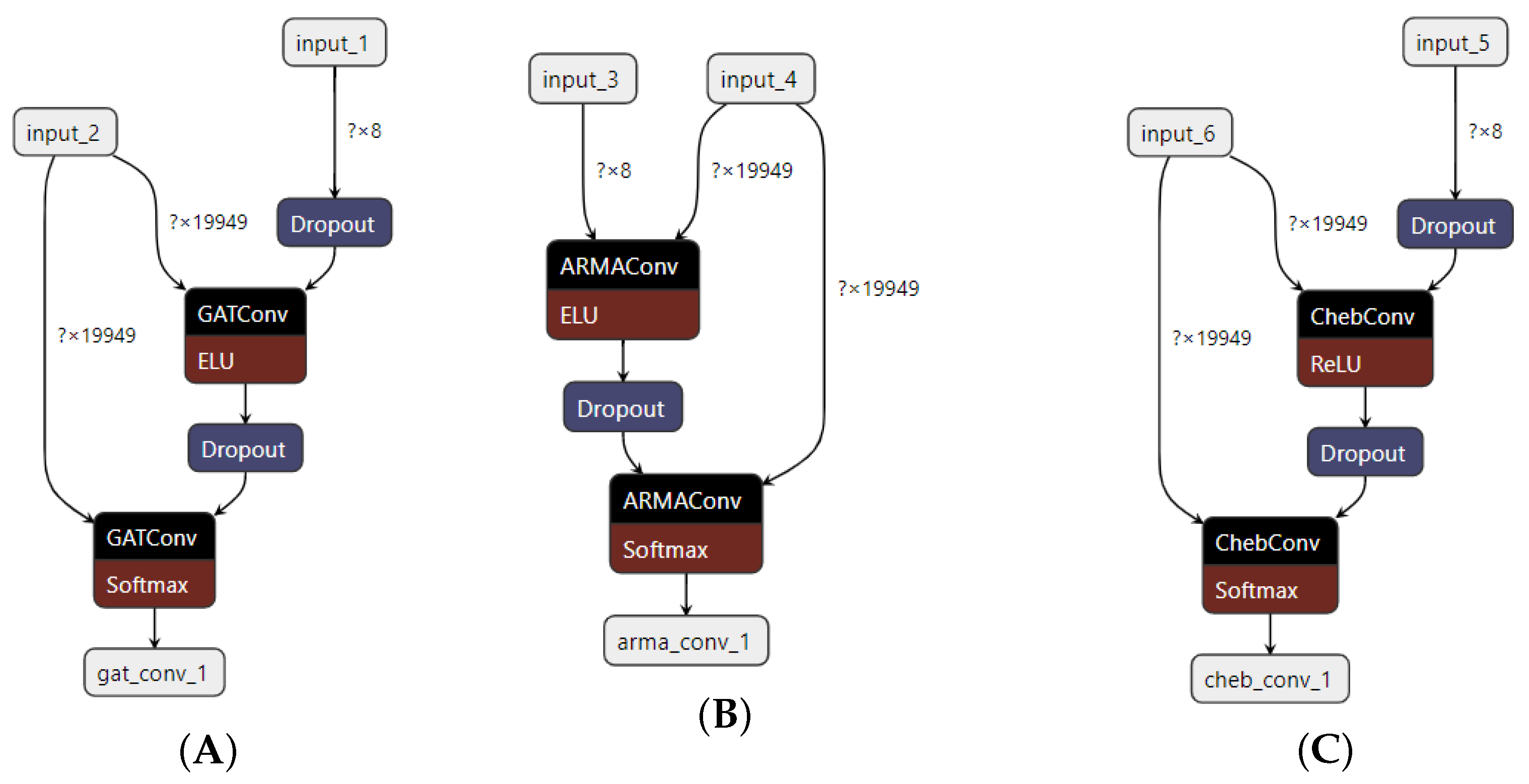
In Figure 1, we present the structures of GAT, ARMA, and Chebyshev graph neural networks (it is not common to represent GraphSage as a diagram). In the presented neural network diagrams, question marks are used to represent the dimensions of the input or output data, rather than specific values. This is because the exact dimensions of the data may vary depending on the specific problem or dataset being used, and the diagrams are meant to convey the general structure of the network, rather than the specific values it will be working with. The use of question marks in these diagrams is a common convention in the field of machine learning and artificial intelligence, as they allow the diagram to be more general and applicable to a wide range of different problems and datasets. Another reason to use question marks is that they allow showing the expected format of the input, without going into the details of the specific data. This means that the network architecture is designed to handle an input of a certain shape, without specifying how that input is going to be.
4. Experiment Description
4.1. Data Preparation
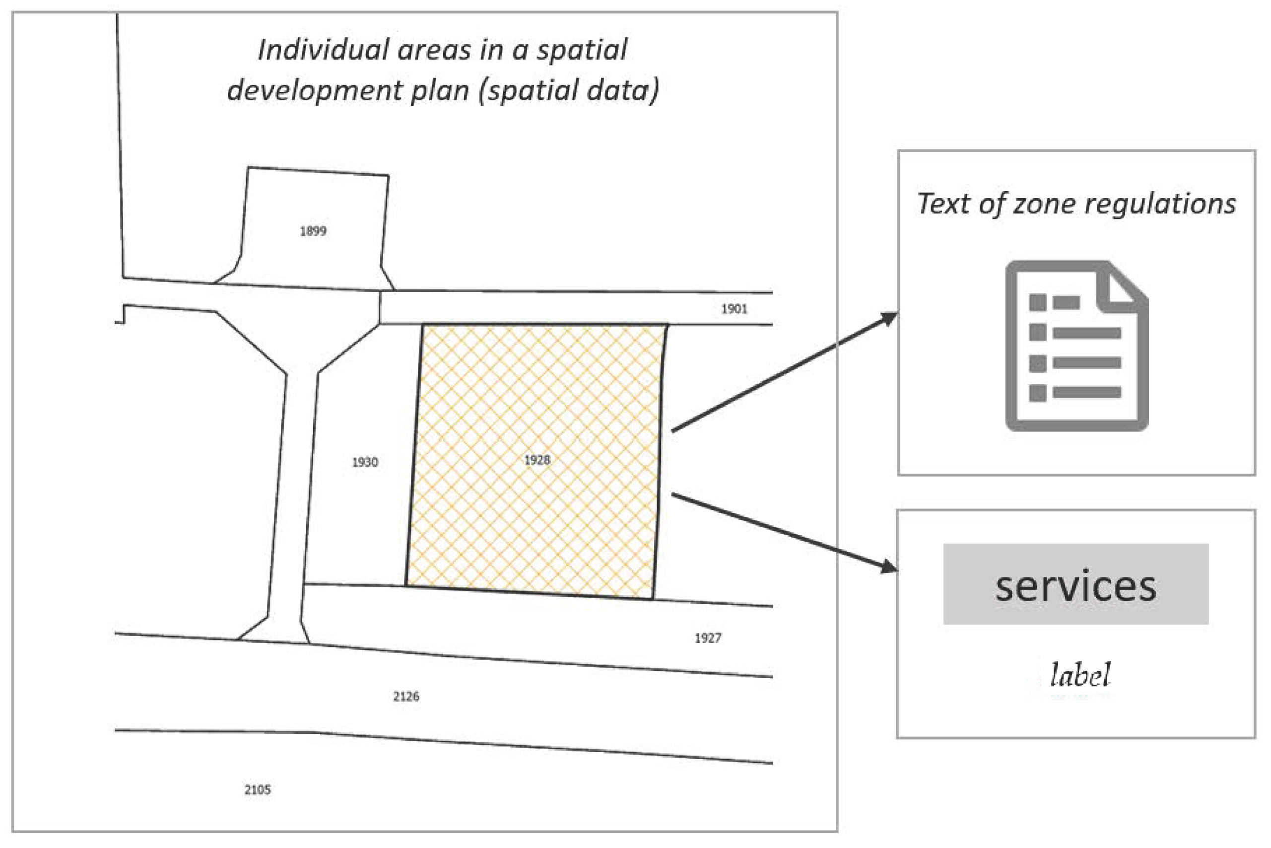
The data obtained for the purposes of the work included 19,948 spatial objects, i.e., planning zones along with their corresponding texts. The texts were detailed provisions for each spatial object (see Figure 2). Depending on the method used, the prepared data had different representations. In the experiments described in Section 4.2.1, the data only included the texts of the detailed plans. In the experiments described in Section 4.2.2, both text data and a neighborhood matrix of the planning zones were used. In the experiments described in Section 4.2.3, the training data were prepared in the form of a graph containing information about the mutual neighborhood of the planning zones, the category of the zone, and its textual description. The preparation of the training data required labeling the category of land use for the planning zones. Due to the lack of a standard for a uniform classification of future land use in plans, it was necessary to adopt a simplified classification for all zones. The labels for the training data were, therefore, categories of land use, from which 8 classes were defined: agriculture, communication and infrastructure, forestry, housing, mining and quarrying, natural areas, production, and services.
4.2. Assumptions for the Experiments
The machine learning algorithms for supervised learning were trained using the Sentence Transformers, TensorFlow, Stellargraph, Spektral, and NetworkX libraries in Python 3.7. In the learning process, homogeneous areas of municipalities were selected in order to maintain the spatial relationship between objects. As a result, 14 consistent regions were distinguished. We applied the cross-validation technique using 7 folds to evaluate the performance of our models.
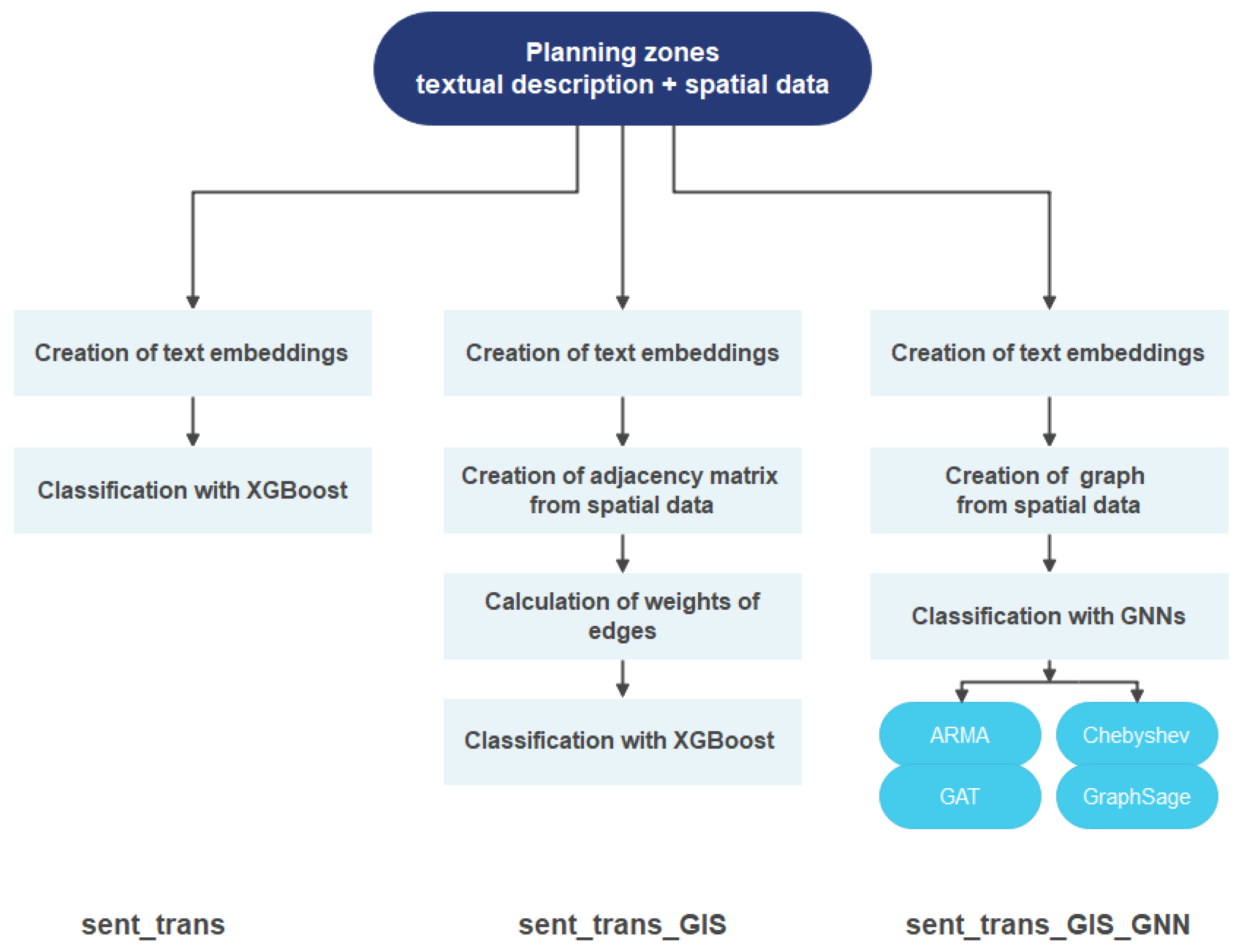
In the experiments presented below, variants were used that differed in the length of the training text data. Tests were performed for the first 35, 50, 100, 150, 200, and 300 words in the texts of local plan provisions. The following subsections describe the classification methods for spatial objects and the experiments performed in this regard. The proposed flowchart for all methods is shown in Figure 3. In the method described in Section 4.2.1, named the sent_trans method, the training data consisted only of the texts of the plans. In the method described in Section 4.2.2, named the sent_trans_GIS method, the training data included the texts of the plans and the adjacency matrix of the objects. In the method described in Section 4.2.3, named the sent_trans_GIS_GNN method, the training data included the text of the plans and the topology of the spatial objects, represented as a graph.
4.2.1. Classification of Spatial Objects Based on Text
In this method, a classifier was created using the corpus of the plan texts as the input data. The vector representation of the text data was created using an embedding generated using the Sentence Transformers model. Sentence Transformers are a type of neural network model that allows for creating numerical representations of sentences or text fragments, called embeddings. In this work, we used the language-independent BERT sentence embedding model, which is a version of BERT. It has been trained to generate embeddings, that is numerical representations of sentences or paragraphs of text in a way that is not specific to any particular language. This means that the model can be used to generate embeddings for text in any language, as long as it is entered in the appropriate format. The dimension of the embedding vector was 768. The XGBoost algorithm was used to classify the texts [32].
4.2.2. Classification of Spatial Objects Based on Text and Adjacency Matrix
In this method, the training data included not only the corpus of the texts, but also aggregated information about the direct neighborhood of the planning zones based on the adjacency matrix. The adjacency matrix of the planning zones was developed for two variants. The adjacency matrix is the sum of two pieces of information. The first is information about which areas are neighbors, and the second is about the potential strength of the interaction between them (the weight value). In the first variant, in the adjacency matrix, spatial objects had equal weight values, i.e., values of 1, in the case of having a neighbor, and 0, in the case of no neighbor. In the second case, the spatial weight value of the neighborhood was based on the adjacency of the objects (common boundary). A common boundary of the objects being compared is understood as a common segment of non-zero length. The individual weights are defined as the ratio of the length of the common boundary of two neighboring areas to the perimeter of the given area. The weights are not symmetrical. Despite the common boundary, the perimeter of the areas is different, so two neighboring objects sharing the same boundary may have different weights. If the area is adjacent to at least two areas of the same category, the weight is the sum of the weights of both of these objects. Like in the previous experiment, the embedding was created using the language-agnostic BERT sentence embedding model, and XGBoost was used as a classifier.
4.2.3. Classification of Spatial Objects Based on Text and Topology of Objects
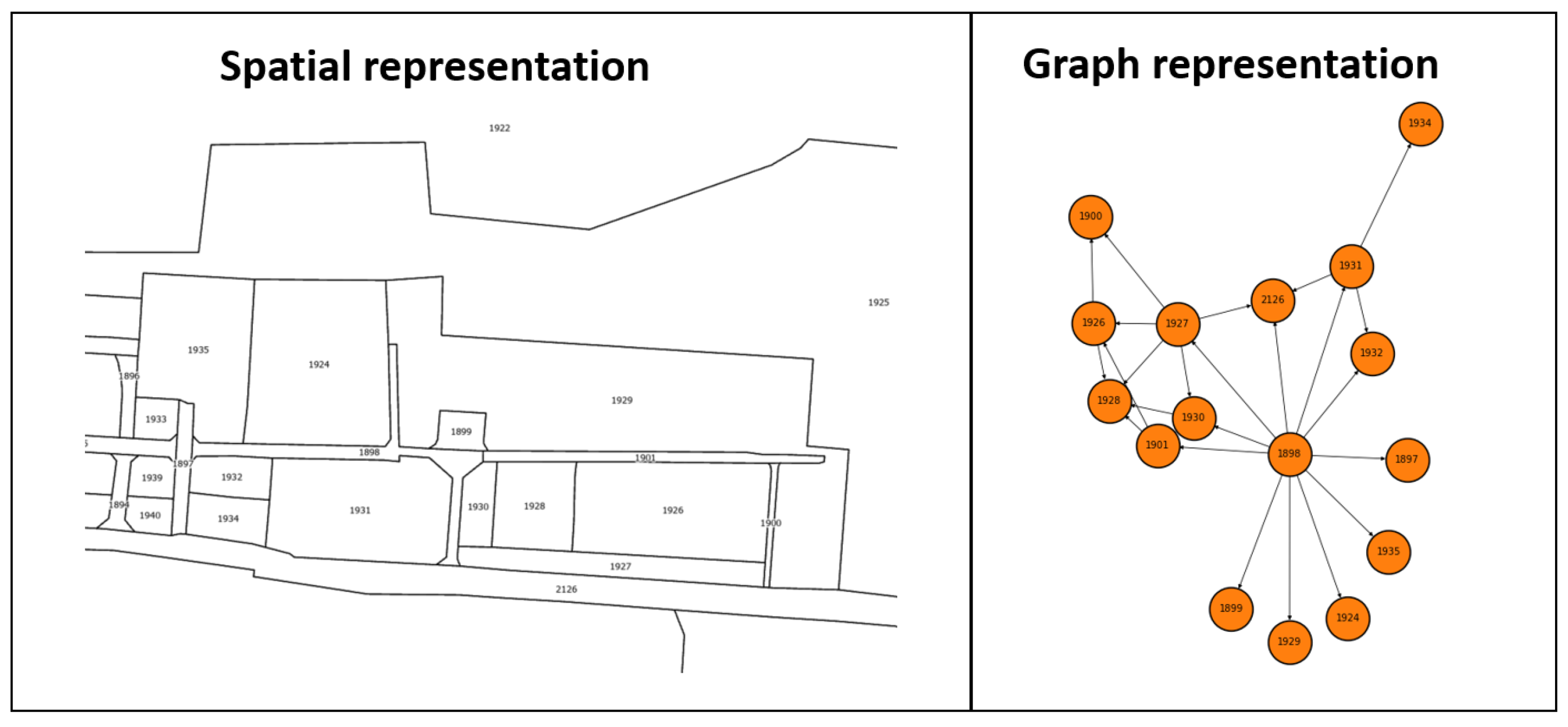
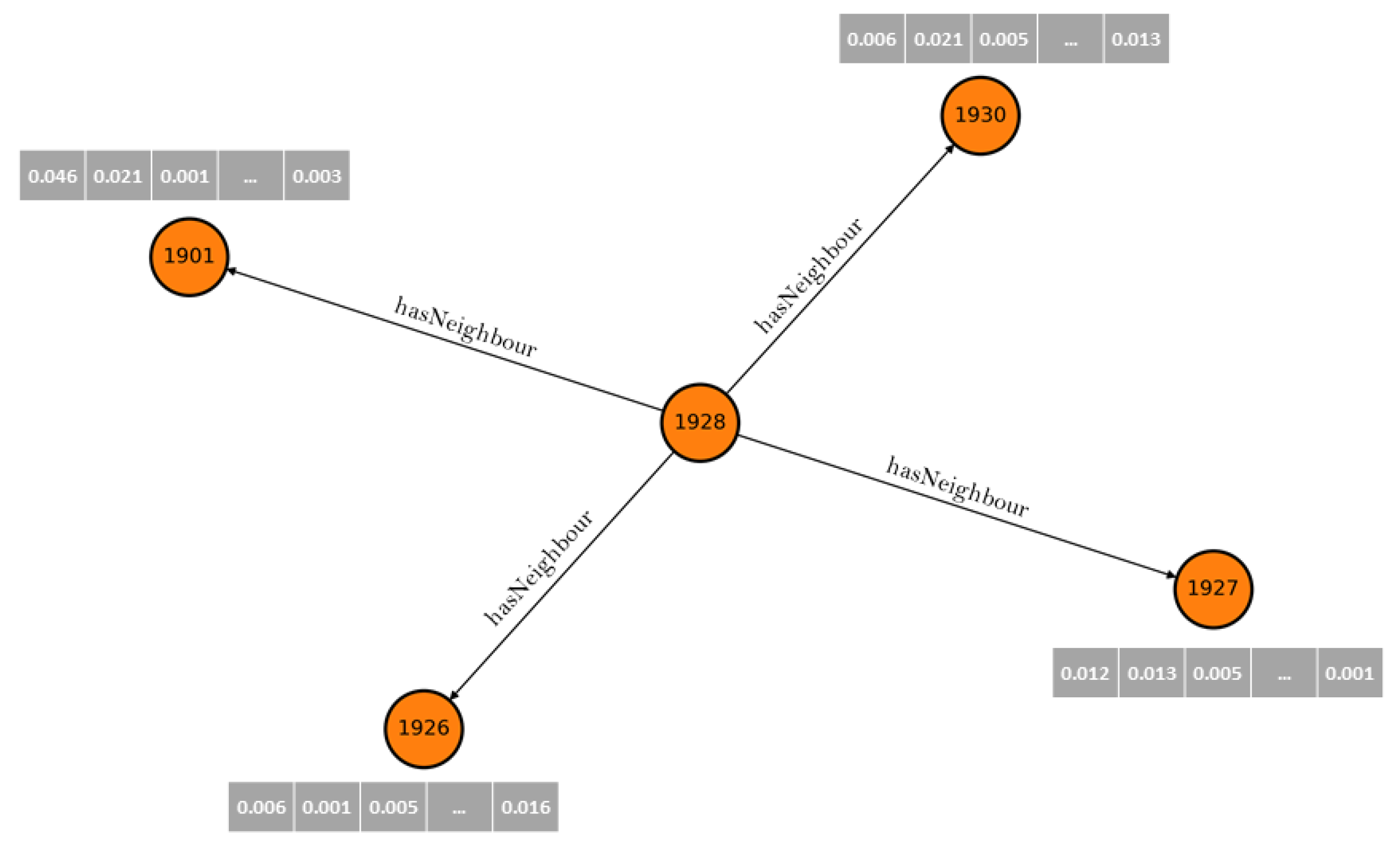
The training data used in this method consisted of spatial and text data, which were represented as a graph. The graph was based on the geometry of the spatial objects, their topology, and the text description (Figure 4). Each node in this graph corresponds to the identifier of the object, its land use category, and the text description.
The textual description is represented in the form of an embedding, created, as in previous methods, with the use of sentence Transformers. The edges, on the other hand, describe the neighborhood relationships between the planning zones (see Figure 5). Thus, by writing the data in the form of a graph, it is possible to represent the full topology of the spatial objects.
The experiments were performed for the four neural network structures described in Section 3, namely GAT, ARMA, Chebyshev, and GraphSage.
5. Results and Discussion
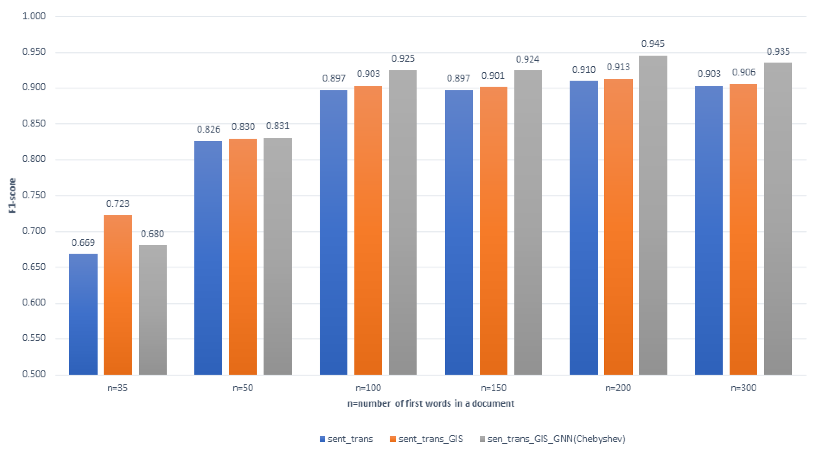
The following drawings show the results of the evaluation of the methods developed in Section 4. Figure 6 shows the values of the F1 measure, which is the harmonic mean of the precision and recall for different document lengths, using semantic Transformer embeddings, an XGBoost classifier, and graph neural networks (Chebyshev). The sent_trans method described in Section 4.2.1 uses only the plan documents as the training data. The sent_trans_GIS method described in Section 4.2.2 takes into account the spatial neighborhood information in the form of an aggregated neighborhood matrix. The sent_trans_GIS_GNN method uses a Chebyshev model based on the graph neural networks described in Section 4.2.3, in which spatial data and text representation in the form of embeddings are stored in the form of a graph.
It can be noticed that there are diverse F1-scores for the above-mentioned methods in different document length categories. For the shortest documents (), poor F1 results were achieved with all three methods, ranging from 0.669 for text-only classification to 0.723 for the use of a neighborhood matrix and 0.680 for GNNs. For the document length , the F1 value was similar for all three methods and oscillated within the range of 0.826–0.831. For document lengths greater than 100 words, the model using graph neural networks outperformed the others, achieving F1 values of 0.925 for 100 words, 0.924 for 150, 0.945 for 200 words, and 0.935 for 300 words. It is worth noting that, for a document length of 200 and 300 words, the other two models, namely the model using only text and the model using the spatial object neighborhood matrix, had lower quality, with an F1 value of 0.897 to 0.913, compared to the graph neural-network-based model, where the F1 value was, respectively, 0.945 and 0.935.
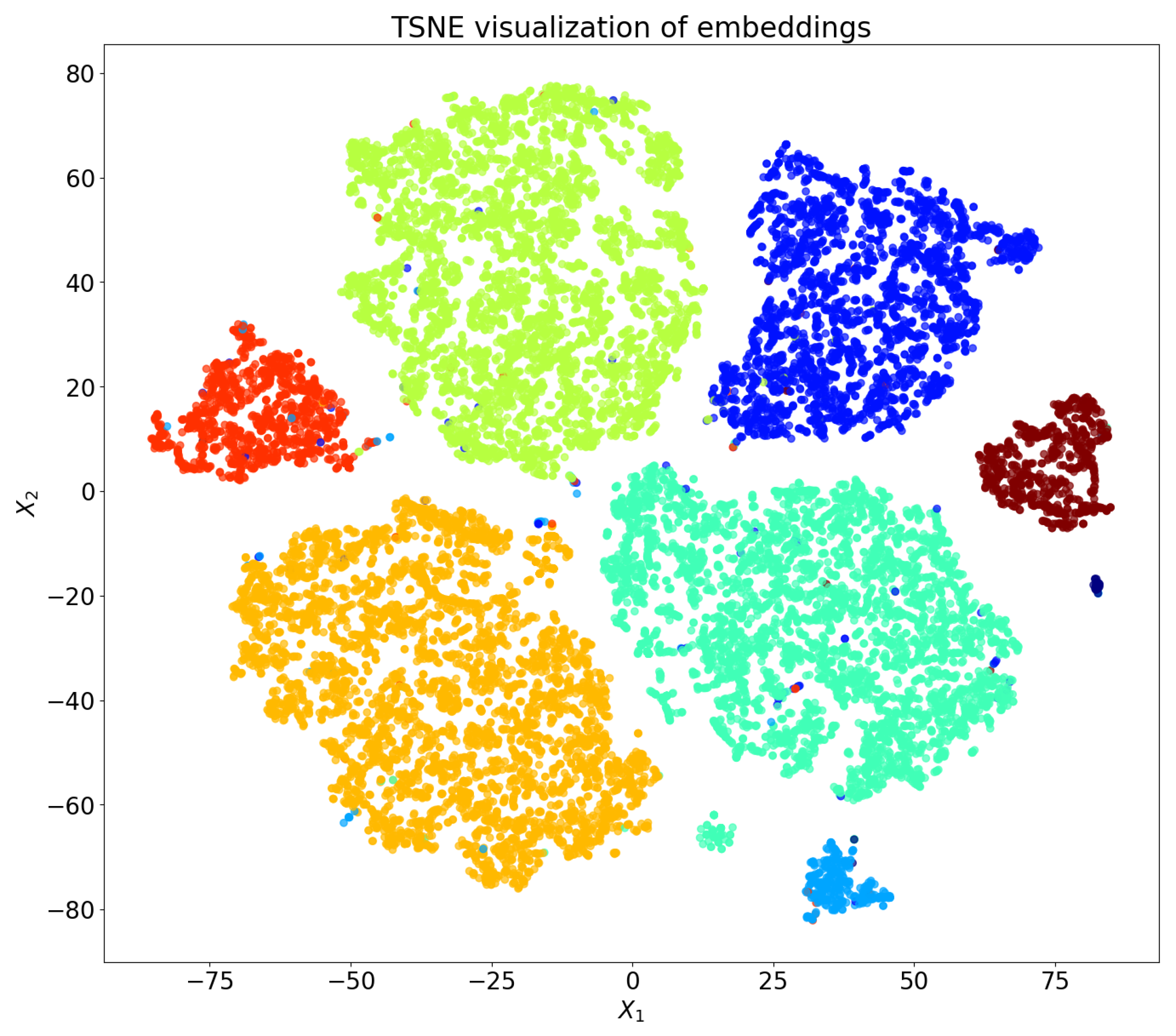
An example visualization of the classification results is shown in Figure 7, where the classification of objects according to the method from Section 4.2.1 is presented. The dimension of the embedding vector was reduced to two using principal component analysis (PCA), and the category labels were assigned the corresponding colors.
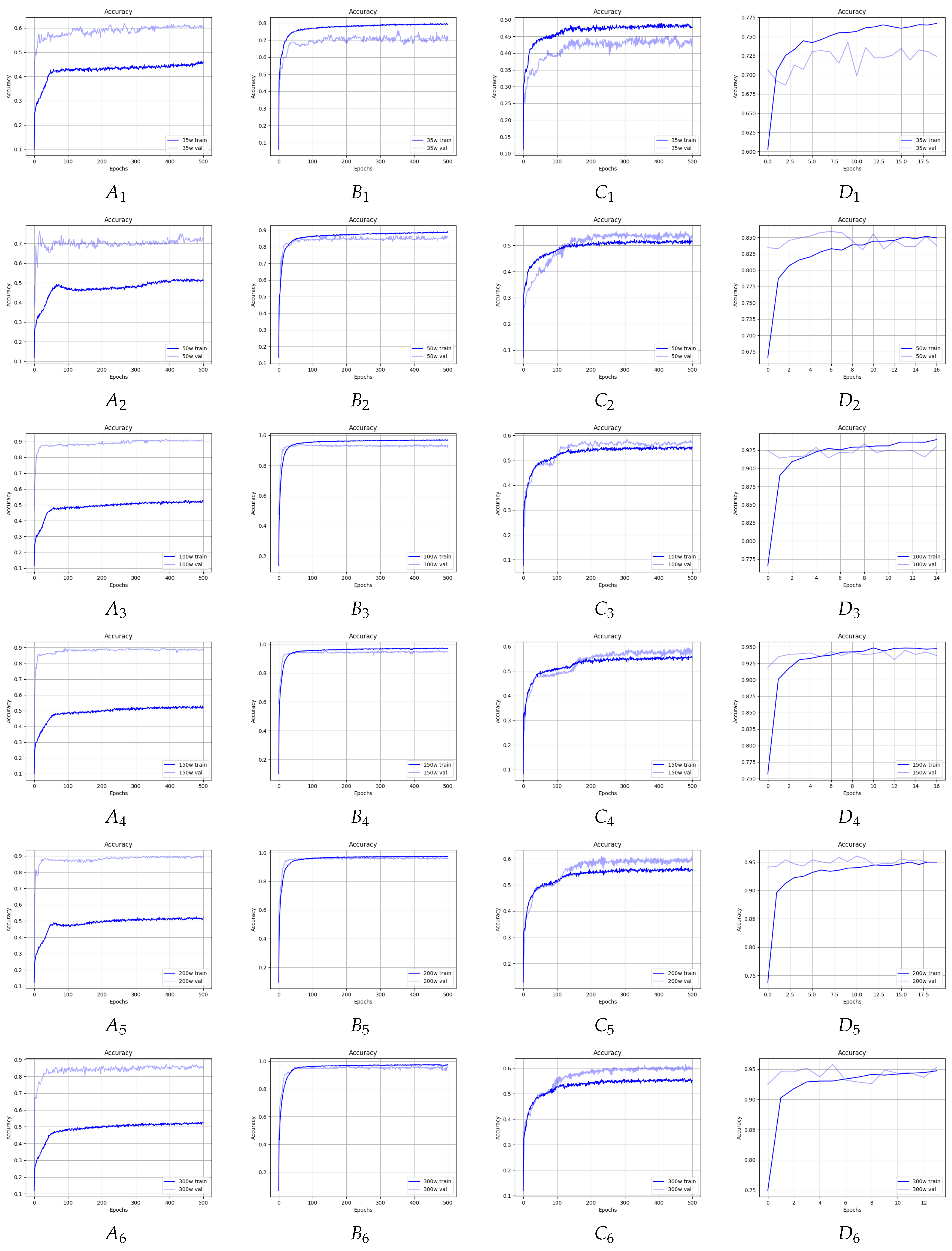
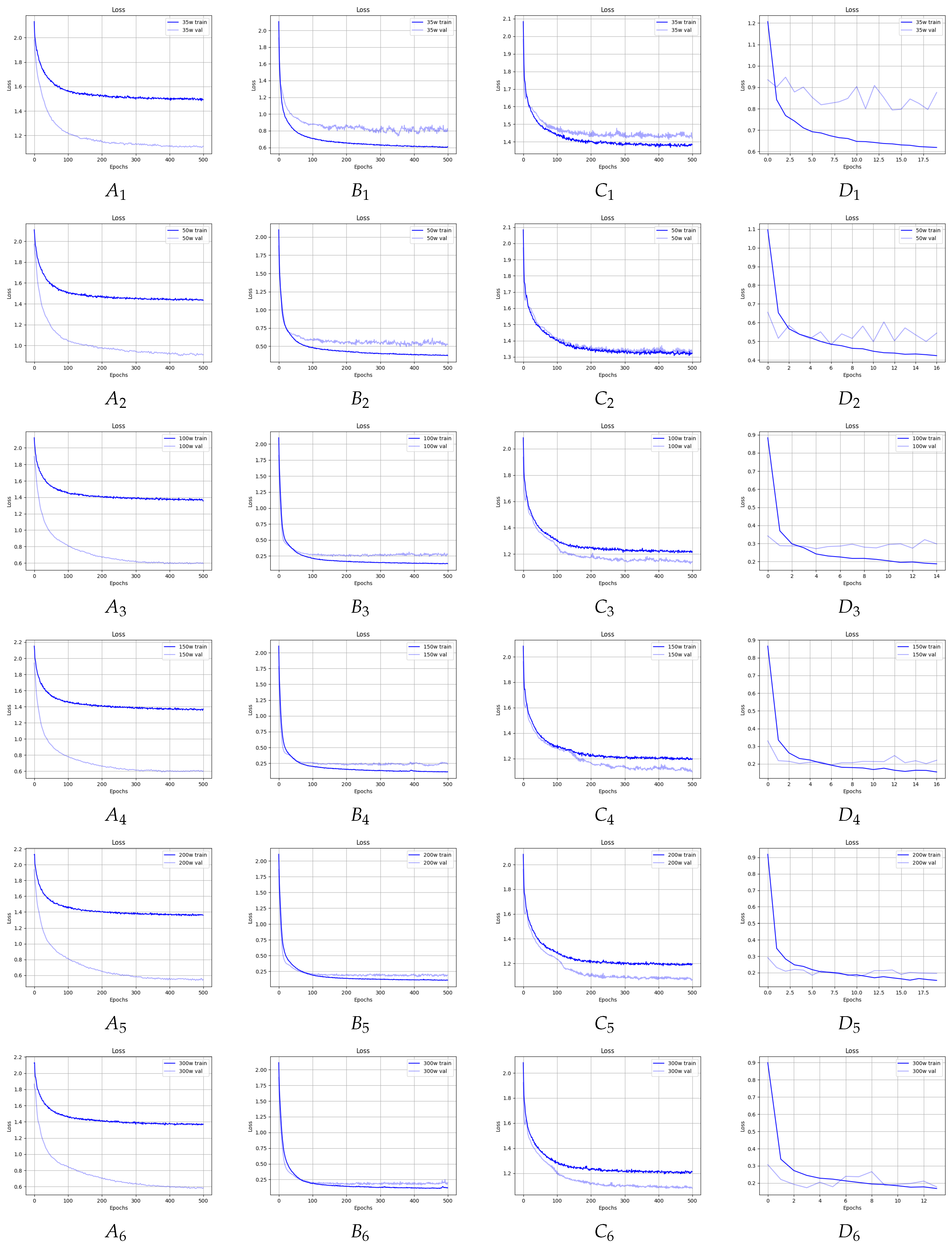
Figure 8 and Figure 9 shows the waveforms of the accuracy and loss functions for the training and validation sets for all considered GNNs and for all considered lengths of the input sequences. In the case of the ARMA, Chebyshev, and GAT models, it was necessary to train for up to 500 epochs to obtain satisfactory accuracy and loss values for the training and validation sets, while in the case of the GraphSage model, about 20 epochs turned out to be sufficient, after which, further training led to overtraining. Observing the accuracy and loss waveforms, we can see that, when classifying texts with a length of 35, the models were usually overtrained, but shorter training resulted in poor accuracy. For texts with a length of 50 or more, we obtained correctly trained models.
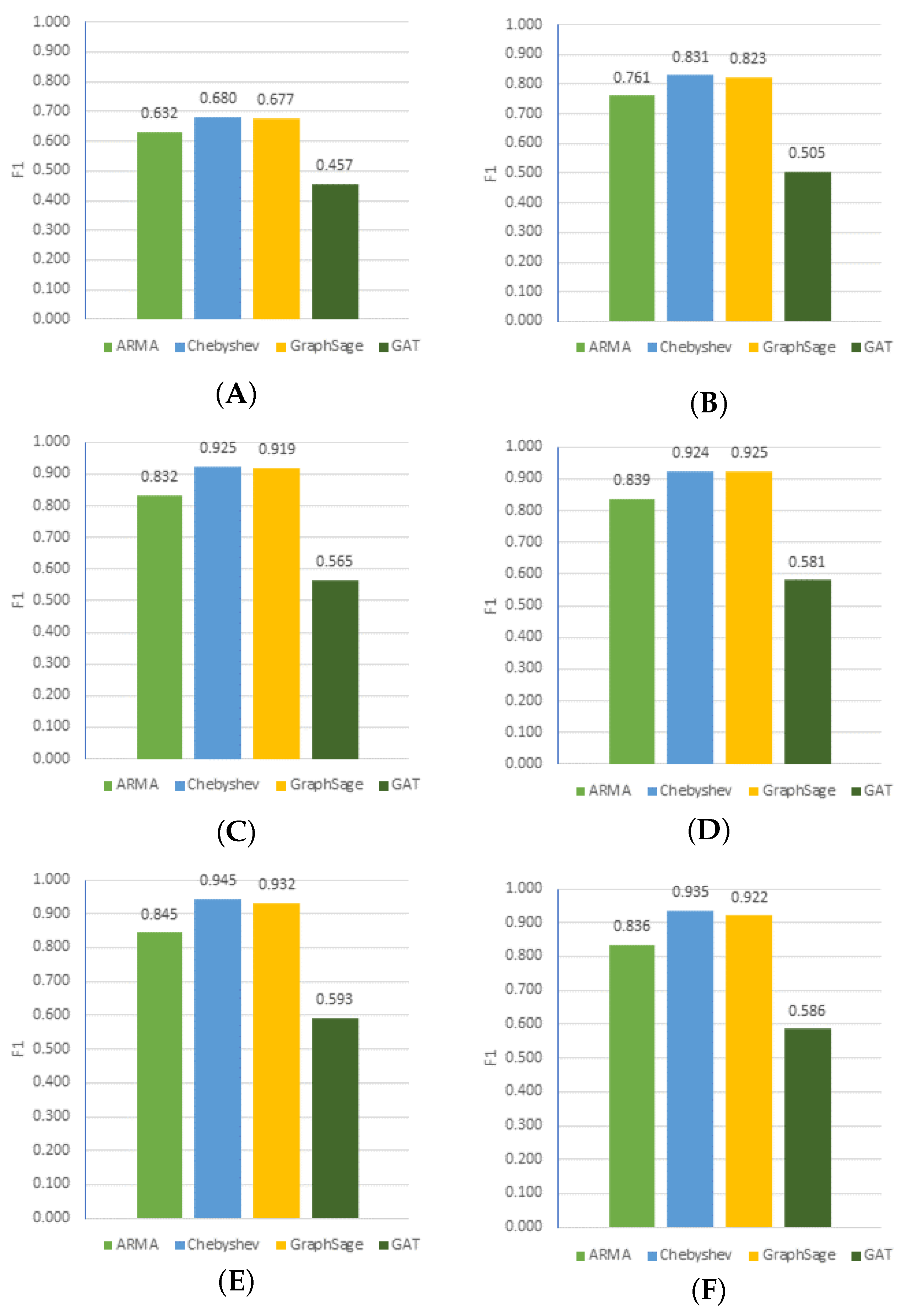
Figure 10 shows the F1 values for all tested graph neural network architectures using different document lengths. The best quality was achieved by the Chebyshev model, with an F1 measure of 0.945 for document lengths . It can be seen that the results were slightly worse at a 300 word length than at a 200 word length. It can be noticed that the best results occurred with document lengths of 200. This situation resulted from the fact that the key information about the land use of the planning zones was at the beginning of the document, which is consistent with the way of formulating text arrangements for individual areas in the plans. Such models that are used to classify documents can be sensitive to the document length because longer documents can contain more information and be more difficult to classify.
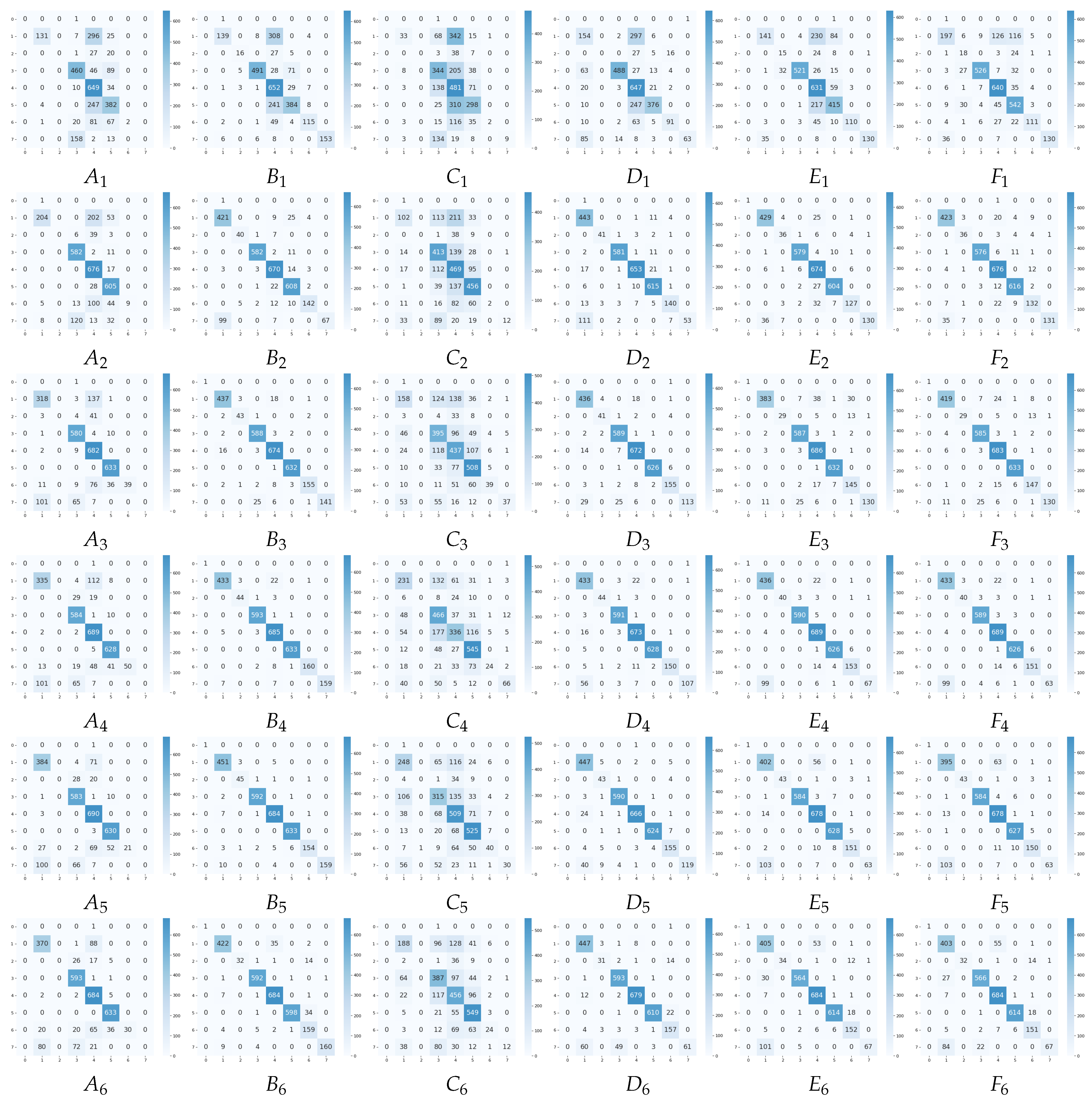
Figure 11 shows selected confusion matrices for the ARMA, Chebyshev, GraphSage, and XGBoost models. For each model, we chose two matrices with the best results (in our opinion), for different lengths of the analyzed texts: ARMA for 150 and 200 words, Chebyshev for 150 and 200 words, GraphSage for 200 and 300 words, and XGBoost for 150 and 200 words. By analyzing all the matrices, for all the considered lengths of the analyzed texts, it can be seen that the quality of the classification improved with the increase in the number of words. Analyzing the matrices, we can observe a high imbalance in the data that we considered, which usually strongly affects the quality of the classifier. In this case, taking into account information about the vicinity of objects significantly improved the quality of the classifiers. Additionally, it is possible to observe that the ARMA model did not detect the seventh class even for a larger number of words. Surprisingly, the Chebyshev neural network recognized this class for a smaller number of considered words. However, due to the small number of texts in this class, it can be seen that it was a problem for most models.
To compare the efficiency of trained models, we executed pairwise paired t-tests with the Benjamini–Hochberg correction for multiple comparisons at the 95% confidence level [33]. For this purpose, we randomly repeated the selection of seven folds for the models’ evaluation three times. The results were used to conduct a statistical test. We found that the Cheby GNN outperformed all other models with its mean F1-score equal to 0.945. The second-best model was GraphSage (F1 = 0.935), which was indistinguishable in the t-test from Cheby (F1 = 0.913, p = 0.252), but worked better than XGBoost (F1 = 0.910, p = 0.021) and less efficient than GAT (p < 0.001) and ARMA (p < 0.001). The baseline GAT model was the least-successful model with its poor performance (F1 = 0.60). The ARMA model (F1 = 0.846) worked much better than GAT, but was beaten by all other approaches. The results of the tests are presented in Table 1.
6. Conclusions
In summary, the classification method based on GNNs presented in this article gave better results than the methods based solely on spatial objects represented as text embeddings or text embeddings with an adjacency matrix only. These conclusions were confirmed by the statistical tests. Testing the algorithms on short texts was intended to check the impact of neighborhood information on the classification result. Reducing the length of the text caused a deterioration in the classification results for the methods using embedding and highlighted the importance of topological information for classification quality.
The conducted experiments clearly indicated that topological information is important in the process of classifying spatial objects. The developed method was tested for spatial objects such as planning zones in spatial development plans. The specificity of spatial planning is holistic, and the functions of neighboring lands are interdependent. However, we believe it is universal and can be applied to other vector data, where objects’ geometry and topology are represented as a graph and object features are written in the form of embeddings.
The method using text and the adjacency matrix, although it gave good results, had limited application only to individual objects. Information about the categories of adjacent areas is required as the input data for prediction. Therefore, in the case of the need to predict a category of land use for the entire area, not a single object, this method is not applicable. It is different in the case of the method based on GNNs, where the adjacency matrix is not required and the prediction of new categories is based on the created graph and object features represented as embeddings.
Combining spatial information with lexical knowledge bases is a tempting direction of development. Sajjadian and Scheider [34] used WordNet to enrich the content of users’ queries in geodata source retrieval. We plan to use the Polish WordNet [35] to describe the predicates of the spatial graph using lexical information, which in combination with the language model (in a hybrid approach) should bring interesting results.
Author Contributions
Conceptualization, Iwona Kaczmarek; methodology, Iwona Kaczmarek, Adam Iwaniak, and Aleksandra Świetlicka; software, Aleksandra Świetlicka and Adam Iwaniak; validation, Adam Iwaniak and Iwona Kaczmarek; formal analysis, Iwona Kaczmarek, Aleksandra Świetlicka, and Adam Iwaniak; investigation, Iwona Kaczmarek, Aleksandra Świetlicka, and Adam Iwaniak; resources, Iwona Kaczmarek; data curation, Iwona Kaczmarek and Adam Iwaniak; writing—original draft preparation, Iwona Kaczmarek and Aleksandra Świetlicka; writing—review and editing, Iwona Kaczmarek, Aleksandra Świetlicka, and Adam Iwaniak; visualization, Aleksandra Świetlicka; supervision, Adam Iwaniak; project administration, Adam Iwaniak; funding acquisition, Adam Iwaniak. All authors have read and agreed to the published version of the manuscript.
Funding
This research was funded by The National Centre for Research and Development in Poland under the POIR.01.01.01-00-0359/20 project ”TeleCyfro”—methods of automated data extraction from analog unstructured engineering documentation using AI in remote work environment. The work was also financed by the research grant No. 0211/SBAD/0122 by Poznan University of Technology.
Institutional Review Board Statement
Not applicable.
Informed Consent Statement
Not applicable.
Data Availability Statement
Restrictions apply to the availability of these data. The data used for the purposes of this article were obtained by the authors under a closed license without the right to further distribution.
Conflicts of Interest
The authors declare no conflict of interest.
References
- Kim, C. Spatial Data Mining, Geovisualization. In International Encyclopedia of Human Geography; Kitchin, R., Thrift, N., Eds.; Elsevier: Oxford, UK, 2009; pp. 332–336. [Google Scholar] [CrossRef]
- Kaczmarek, I.; Iwaniak, A.; Świetlicka, A.; Piwowarczyk, M.; Nadolny, A. A machine learning approach for integration of spatial development plans based on natural language processing. Sustain. Cities Soc. 2022, 76, 103479. [Google Scholar] [CrossRef]
- Reimers, N.; Gurevych, I. Sentence-BERT: Sentence Embeddings using Siamese BERT-Networks. arXiv 2019, arXiv:1908.10084. [Google Scholar] [CrossRef]
- Reimers, N.; Gurevych, I. Making Monolingual Sentence Embeddings Multilingual using Knowledge Distillation. In Proceedings of the 2020 Conference on Empirical Methods in Natural Language Processing, Online, 19–20 November 2020; Association for Computational Linguistics: Toronto, ON, Canada, 2020. [Google Scholar]
- Li, Y.; Zhang, H.; Xue, X.; Jiang, Y.; Shen, Q. Deep learning for remote sensing image classification: A survey. WIREs Data Min. Knowl. Discov. 2018, 8, e1264. [Google Scholar] [CrossRef] [Green Version]
- Alem, A.; Kumar, S. Deep Learning Methods for Land Cover and Land Use Classification in Remote Sensing: A Review. In Proceedings of the 2020 8th International Conference on Reliability, Infocom Technologies and Optimization (Trends and Future Directions) (ICRITO), Noida, India, 4–5 June 2020; pp. 903–908. [Google Scholar] [CrossRef]
- Zhu, X.X.; Tuia, D.; Mou, L.; Xia, G.S.; Zhang, L.; Xu, F.; Fraundorfer, F. Deep Learning in Remote Sensing: A Comprehensive Review and List of Resources. IEEE Geosci. Remote Sens. Mag. 2017, 5, 8–36. [Google Scholar] [CrossRef] [Green Version]
- Song, J.; Gao, S.; Zhu, Y.; Ma, C. A survey of remote sensing image classification based on CNNs. Big Earth Data 2019, 3, 232–254. [Google Scholar] [CrossRef]
- Prathap, G.; Afanasyev, I. Deep Learning Approach for Building Detection in Satellite Multispectral Imagery. In Proceedings of the 2018 International Conference on Intelligent Systems (IS), Funchal, Portugal, 25–27 September 2018; pp. 461–465. [Google Scholar] [CrossRef] [Green Version]
- Wambugu, N.; Chen, Y.; Xiao, Z.; Wei, M.; Aminu Bello, S.; Marcato Junior, J.; Li, J. A hybrid deep convolutional neural network for accurate land cover classification. Int. J. Appl. Earth Obs. Geoinf. 2021, 103, 102515. [Google Scholar] [CrossRef]
- Gori, M.; Monfardini, G.; Scarselli, F. A new model for learning in graph domains. In Proceedings of the Proceedings. 2005 IEEE International Joint Conference on Neural Networks, Montreal, QC, Canada, 31 July–4 August 2005; Volume 2, pp. 729–734. [Google Scholar] [CrossRef]
- Scarselli, F.; Gori, M.; Tsoi, A.C.; Hagenbuchner, M.; Monfardini, G. The Graph Neural Network Model. IEEE Trans. Neural Netw. 2009, 20, 61–80. [Google Scholar] [CrossRef] [Green Version]
- Stokes, J.M.; Yang, K.; Swanson, K.; Jin, W.; Cubillos-Ruiz, A.; Donghia, N.M.; MacNair, C.R.; French, S.; Carfrae, L.A.; Bloom-Ackermann, Z.; et al. A Deep Learning Approach to Antibiotic Discovery. Cell 2020, 180, 688–702.e13. [Google Scholar] [CrossRef] [Green Version]
- Yang, K.; Swanson, K.; Jin, W.; Coley, C.; Eiden, P.; Gao, H.; Guzman-Perez, A.; Hopper, T.; Kelley, B.; Mathea, M.; et al. Analyzing Learned Molecular Representations for Property Prediction. J. Chem. Inf. Model. 2019, 59, 3370–3388. [Google Scholar] [CrossRef] [Green Version]
- Derrow-Pinion, A.; She, J.; Wong, D.; Lange, O.; Hester, T.; Perez, L.; Nunkesser, M.; Lee, S.; Guo, X.; Wiltshire, B.; et al. ETA Prediction with Graph Neural Networks in Google Maps. In Proceedings of the 30th ACM International Conference on Information & Knowledge Management, Online, 1–5 November 2021; ACM: New York, NY, USA, 2021. [Google Scholar] [CrossRef]
- Danel, T.; Spurek, P.; Tabor, J.; Śmieja, M.; Struski, Ł.; Słowik, A.; Maziarka, Ł. Spatial Graph Convolutional Networks. arXiv 2019, arXiv:1909.05310. [Google Scholar] [CrossRef]
- Klemmer, K.; Safir, N.; Neill, D.B. Positional Encoder Graph Neural Networks for Geographic Data. arXiv 2021, arXiv:2111.10144. [Google Scholar] [CrossRef]
- Xu, Y.; Jin, S.; Chen, Z.; Xie, X.; Hu, S.; Xie, Z. Application of a graph convolutional network with visual and semantic features to classify urban scenes. Int. J. Geogr. Inf. Sci. 2022, 36, 2009–2034. [Google Scholar] [CrossRef]
- Jiang, W.; Luo, J. Graph neural network for traffic forecasting: A survey. Expert Syst. Appl. 2022, 207, 117921. [Google Scholar] [CrossRef]
- Yan, J.; Ji, S.; Wei, Y. A Combination of Convolutional and Graph Neural Networks for Regularized Road Surface Extraction. IEEE Trans. Geosci. Remote Sens. 2022, 60, 1–13. [Google Scholar] [CrossRef]
- Lan, T.; Cheng, H.; Wang, Y.; Wen, B. Site Selection via Learning Graph Convolutional Neural Networks: A Case Study of Singapore. Remote Sens. 2022, 14, 3579. [Google Scholar] [CrossRef]
- Sen, P.; Namata, G.; Bilgic, M.; Getoor, L.; Galligher, B.; Eliassi-Rad, T. Collective Classification in Network Data. AI Mag. 2008, 29, 93. [Google Scholar] [CrossRef] [Green Version]
- Grattarola, D.; Alippi, C. Graph Neural Networks in TensorFlow and Keras with Spektral. arXiv 2020, arXiv:2006.12138. [Google Scholar] [CrossRef]
- CSIRO’s Data61. StellarGraph Machine Learning Library. GitHub Repository 2018. [Google Scholar]
- Kipf, T.N.; Welling, M. Semi-Supervised Classification with Graph Convolutional Networks. arXiv 2016, arXiv:1609.02907. [Google Scholar] [CrossRef]
- Hamilton, W.L.; Ying, R.; Leskovec, J. Inductive Representation Learning on Large Graphs. arXiv 2017, arXiv:1706.02216. [Google Scholar] [CrossRef]
- Vaswani, A.; Shazeer, N.; Parmar, N.; Uszkoreit, J.; Jones, L.; Gomez, A.N.; Kaiser, L.; Polosukhin, I. Attention Is All You Need. arXiv 2017, arXiv:1706.03762. [Google Scholar] [CrossRef]
- Bahdanau, D.; Cho, K.; Bengio, Y. Neural Machine Translation by Jointly Learning to Align and Translate. arXiv 2014, arXiv:1409.0473. [Google Scholar] [CrossRef]
- Gehring, J.; Auli, M.; Grangier, D.; Dauphin, Y.N. A Convolutional Encoder Model for Neural Machine Translation. arXiv 2016, arXiv:1611.02344. [Google Scholar] [CrossRef]
- Bianchi, F.M.; Grattarola, D.; Livi, L.; Alippi, C. Graph Neural Networks with Convolutional ARMA Filters. IEEE Trans. Pattern Anal. Mach. Intell. 2021, 44, 3496–3507. [Google Scholar] [CrossRef]
- Defferrard, M.; Bresson, X.; Vandergheynst, P. Convolutional Neural Networks on Graphs with Fast Localized Spectral Filtering. arXiv 2016, arXiv:1606.09375. [Google Scholar] [CrossRef]
- Chen, T.; Guestrin, C. XGBoost: A Scalable Tree Boosting System. In Proceedings of the KDD’16: 22nd ACM SIGKDD International Conference on Knowledge Discovery and Data Mining, San Francisco, CA, USA, 13–17 August 2016; ACM: New York, NY, USA, 2016; pp. 785–794. [Google Scholar] [CrossRef] [Green Version]
- Benjamini, Y.; Hochberg, Y. Controlling the False Discovery Rate: A Practical and Powerful Approach to Multiple Testing. J. R. Stat. Soc. Ser. B (Methodol.) 1995, 57, 289–300. [Google Scholar] [CrossRef]
- Sajjadian, M.; Scheider, S. Geodata source retrieval by multilingual/semantic query expansion: The Case of Google Translate and WordNet version 3.1. AGILE GISci. Ser. 2022, 3, 60. [Google Scholar] [CrossRef]
- Maziarz, M.; Piasecki, M.; Rudnicka, E.; Szpakowicz, S.; Kędzia, P. plWordNet 3.0—A Comprehensive Lexical-Semantic Resource. In Proceedings of COLING 2016, the 26th International Conference on Computational Linguistics: Technical Papers; The COLING 2016 Organizing Committee: Osaka, Japan, 2016; pp. 2259–2268. [Google Scholar]
Figure 1.
Structures of examined graph neural networks: (A) GAT, (B) ARMA, and (C) Chebyshev.

Figure 2.
Representation of the data.

Figure 3.
Flowchart of the proposed methods.

Figure 4.
Spatial and graph representation of spatial objects.

Figure 5.
Representation of spatial objects in the form of a graph.

Figure 6.
Comparison of F1-score for three different classification models for spatial objects.

Figure 7.
T-SNE visualization of the embedding matrix generated with the language-agnostic BERT sentence embedding model.
Figure 7.
T-SNE visualization of the embedding matrix generated with the language-agnostic BERT sentence embedding model.

Figure 8.
Accuracy waveforms for the (A) ARMA, (B) Chebyshev, (C) GAT, and (D) GraphSage models, which considered: 1. 35, 2. 50, 3. 100, 4. 150, 5. 200, and 6. 300 words.
Figure 8.
Accuracy waveforms for the (A) ARMA, (B) Chebyshev, (C) GAT, and (D) GraphSage models, which considered: 1. 35, 2. 50, 3. 100, 4. 150, 5. 200, and 6. 300 words.

Figure 9.
Loss waveforms for the (A) ARMA, (B) Chebyshev, (C) GAT, and (D) GraphSage models, which considered: 1. 35, 2. 50, 3. 100, 4. 150, 5. 200, and 6. 300 words.
Figure 9.
Loss waveforms for the (A) ARMA, (B) Chebyshev, (C) GAT, and (D) GraphSage models, which considered: 1. 35, 2. 50, 3. 100, 4. 150, 5. 200, and 6. 300 words.

Figure 10.
Comparison of the quality of three graph neural network models, ARMA, Chebyshev, and GraphSAGE, for different document lengths measured by word count. (A) 35, (B) 50, (C) 100, (D) 150, (E) 200, and (F) 300.
Figure 10.
Comparison of the quality of three graph neural network models, ARMA, Chebyshev, and GraphSAGE, for different document lengths measured by word count. (A) 35, (B) 50, (C) 100, (D) 150, (E) 200, and (F) 300.

Figure 11.
Confusion matrices for models: (A) ARMA, (B) Chebyshev, (C) GAT, (D) GraphSage, (E) XGBoost, and (F) XGBoost with the GIS, which considered 1. 35, 2. 50, 3. 100, 4. 150, 5. 200, and 6. 300 words.
Figure 11.
Confusion matrices for models: (A) ARMA, (B) Chebyshev, (C) GAT, (D) GraphSage, (E) XGBoost, and (F) XGBoost with the GIS, which considered 1. 35, 2. 50, 3. 100, 4. 150, 5. 200, and 6. 300 words.


Table 1.
Results of paired pairwise t-tests.
| Model 1 | Model 2 | Fdr_bh |
|---|---|---|
| GAT | Cheby | 0.000 |
| GAT | ARMA | 0.000 |
| GAT | GraphSage | 0.000 |
| GAT | sent_trans_GIS | 0.000 |
| GAT | sent_trans | 0.000 |
| Cheby | ARMA | 0.000 |
| Cheby | GraphSage | 0.252 |
| Cheby | sent_trans_GIS | 0.025 |
| Cheby | sent_trans | 0.021 |
| ARMA | GraphSage | 0.000 |
| ARMA | sent_trans_GIS | 0.000 |
| ARMA | sent_trans | 0.000 |
| GraphSage | sent_trans_GIS | 0.113 |
| GraphSage | sent_trans | 0.101 |
| sent_trans_GIS | sent_trans | 0.101 |
Disclaimer/Publisher’s Note: The statements, opinions and data contained in all publications are solely those of the individual author(s) and contributor(s) and not of MDPI and/or the editor(s). MDPI and/or the editor(s) disclaim responsibility for any injury to people or property resulting from any ideas, methods, instructions or products referred to in the content. |
© 2023 by the authors. Licensee MDPI, Basel, Switzerland. This article is an open access article distributed under the terms and conditions of the Creative Commons Attribution (CC BY) license (https://creativecommons.org/licenses/by/4.0/).
Share and Cite
MDPI and ACS Style
Kaczmarek, I.; Iwaniak, A.; Świetlicka, A. Classification of Spatial Objects with the Use of Graph Neural Networks. ISPRS Int. J. Geo-Inf. 2023, 12, 83. https://doi.org/10.3390/ijgi12030083
AMA Style
Kaczmarek I, Iwaniak A, Świetlicka A. Classification of Spatial Objects with the Use of Graph Neural Networks. ISPRS International Journal of Geo-Information. 2023; 12(3):83. https://doi.org/10.3390/ijgi12030083
Chicago/Turabian StyleKaczmarek, Iwona, Adam Iwaniak, and Aleksandra Świetlicka. 2023. "Classification of Spatial Objects with the Use of Graph Neural Networks" ISPRS International Journal of Geo-Information 12, no. 3: 83. https://doi.org/10.3390/ijgi12030083
Note that from the first issue of 2016, this journal uses article numbers instead of page numbers. See further details here.