Mapping Cropland Extent in Pakistan Using Machine Learning Algorithms on Google Earth Engine Cloud Computing Framework

Abstract

An actual cropland extent product with a high spatial resolution with a precision of up to 60 m is believed to be particularly significant in tackling numerous water security concerns and world food challenges. To advance the development of niche, advanced cropland goods such as crop variety techniques, crop intensities, crop water production, and crop irrigation, it is necessary to examine how cropland products typically span narrow or expansive farmlands. Some of the existing challenges are processing by constructing precision-high resolution cropland-wide items of training and testing data on diverse geographical locations and safe frontiers, computing capacity, and managing vast volumes of geographical data. This analysis includes eight separate Sentinel-2 multi-spectral instruments data from 2018 to 2019 (Short-wave Infrared Imagery (SWIR 2), SWIR 1, Cirrus, the near infrared, red, green, blue, and aerosols) have been used. Pixel-based classification algorithms have been employed, and their precision is measured and scrutinized in this study. The computations and analyses have been conducted on the cloud-based Google Earth Engine computing network. Training and testing data were obtained from the Google Earth Engine map console at a high spatial 10 m resolution for this analysis. The basis of research information for testing the computer algorithms consists of 855 training samples, culminating in a manufacturing field of 200 individual validation samples measuring product accuracy. The Pakistan cropland extent map produced in this study using four state-of-the-art machine learning (ML) approaches, Random Forest, SVM, Naïve Bayes & CART shows an overall validation accuracy of 82%, 89% manufacturer accuracy, and 77% customer accuracy. Among these four machine learning algorithms, the CART algorithm overperformed the other three, with an impressive classification accuracy of 93%. Pakistan’s average cropland areas were calculated to be 370,200 m², and the cropland’s scale of goods indicated that sub-national croplands could be measured. The research offers a conceptual change in the development of cropland maps utilizing a remote sensing multi-date.

1. Introduction

Precise agricultural croplands are of considerable value in assessing and tracking the world’s food and water health in broad regions that chart small to large fields. The presence of humans has already been a significant part of the research on the Earth’s atmosphere [1]. However, stronger relations the with economic and social sciences are required to study the projected population development, migration trends, allocation of food resources, and earth management practice to adapt to current global biodiversity challenges [2]. These methods are also very relevant to assess the worldwide cultivation of water, the productivity of crops (productivity per unit of soil), the productivity of water (crop per drop or productivity per unit of water), and studies regarding food security [3,4,5,6]. The efficient monitoring of crop conditions requires the regional, timely, precise, and cost-effective mapping of croplands. In this case, spatially dispersed remote monitoring maps with high spatial resolution provide a powerful means for the monitoring of croplands [7].

The recent decades have seen a proliferation of global and national cropland devices that make use of the medium to coarse (250 m to 1 km) distant sensing data, such as the (AVHRR) Advanced Very High-Resolution Radio, and the (MODIS) Moderate Resolution Image Spectroradiometer [8,9,10,11,12,13]. Their geographical distribution patterns and features, such as the strength of crops and crop superiority, are highly beneficial to offer an initial evaluation of agricultural croplands. However, the poor resolution of such materials hinders the applicability of these materials in appraising small farms [14]. In addition, the Land Use Land Cover (LULC) products generated using various remote sensing data containing croplands that are agricultural in one or more categories are subject to worldwide regional land utilization. Topics include the MCD12Q1 [15], Global Land Cover Fine Resolution [16], and Globeland30 [17]. However, the LULC-focused goods did not focus on mapping croplands in depth. Cropland accuracy is also affected [18]. Many of these products are often coarse.

Cropland concepts often vary from product to product, with specific cropland outcomes and features for each product. In general, the current cropland scale items are of gross resolution, lack field specifics, or are mapped in certain LULC categories with no emphasis on different cropland classes [19]. Consequently, very high risks and failures exist at cropland locations. In the past, there have been incidences of agricultural cropland monitoring using sophisticated remote-sensing technologies. Such studies were based on numerous sensor data for various irrigated and rain-fed cultures with spectral, radiometric, and spatial-temporal resolutions [8,9,13,20,21,22,23,24,25,26,27]. This approach consists of object-based or pixel-based techniques or a combination of unsupervised and supervised techniques. Pixel-based approaches include: (a) employing a time-weighted dynamic temporal warping analysis based on pixels and objects [20], (b) the Knowledge-Based Temporal Features method [7], (c) the RF Algorithm [22,28], (d) SVM Support Vector Machines [29], (e) the probabilistic method [30], (f) Decision Tree [31,32], (g) Spectral Matching techniques [33,34], and (h) phenomenological approaches [35,36].

A current attempt was made to map the cropland scale to semi-automatics preparation and multi-classification method approaches [37,38]. Nevertheless, such approaches have primarily been applied to: (a) high-resolution (Landsat 30-m) areas, (b) limited areas, and (c) multi-temporal intermediate (250-m or higher) remotely sensed data. Obtaining high-quality, cloud-accessible imagery and using multi-temporal, high-resolution data has previously been challenging for farmland mapping over broad expanses. However, these problems have been eliminated due to a shift in underlying data collection regarding remote sensing, administration, and analysis paradigms. Sentinel-2 routinely collects the high-resolution visual imagery of land and ocean environments (10 m to 60 m) [39]. The Sentinel-2 multi-spectral satellite captures details in 13 invisible, short-wave, short-spectrum frequencies. Sentinel-2 protects the coast and the Mediterranean Sea from 56° S to 84° N. The Sentinel-2 satellite revisits and captures land area imagery of the exact land area coordinates or the same area of land at five day intervals. However, the viewing angles vary. Sentinel-2 captures scenes with room resolutions of 10 m, 20 m, and 60 m [40]. Managing vast amounts of Landsat data for study across broad areas is a primary challenge in modern remote sensing strategies utilizing commercial imagery processing tools on PC-based workstations [41].

Whatever the strength of the devices, the entire data analysis operation, including pre-processing, is complicated, slower, and repetitive in vast areas, including 1000 sentinel-2 images. Large-scale sensing without these limitations is now possible thanks to the advent of the internet and the widespread adoption of high-powered ML algorithms in cloud computing platforms such as the Google Earth Engine [42,43]. Ref. [43] demonstrated that a GEE database that incorporates earth observers and airborne sensors, such as the United States Department of Agriculture (USDA), Moderate Resolution Imaging Spectroradiometer (MODIS), National Agriculture Statistical Service (NASS), National Aeronautics and Space Administration (NASA), Cropland Data Layer(CDL), and the United States Geological Survey (USGS) Landsat, and weather/climate databases, as well as automated elevator templates, can be integrated to include multi-petabyte repositories of georeferenced databases.

This framework’s robust data management has made it applicable to various geospatial processing tasks. GEE allows batch processing using Python or JavaScript on application program interfaces and supports essential machine learning algorithms (MLAs) that are commonly beneficial for image enhancement and picture classification application programming interfaces (APIs). It does away with the need for many pre-processing steps in traditional remote sensing systems. Some research [44] has recently utilized the GEE platform for global and continental-scale mapping projects. Thus, this analysis’s primary objective was to map all croplands comprehensively using high-resolution (up to 60 m), multi-year (2018–2020) (five-days), and multi-spectral instrument (sentinel-2) level-1C data for all of Pakistan. Pakistan has vast fields of cropland with different crop systems. It is a primary producer of agricultural produce and an exporter of large commercial agricultural fields [44].

Significant crops in agriculture, including rice, wheat, cotton, sugarcane, and maize, have recorded 25.6 percent value-added in agriculture and 5.3% of the gross domestic product in Pakistan. Wheat is a major crop in this region’s agricultural industry, accounting for 10% of the value-added agriculture and 2.1% of the gross domestic product [45]. There has been a downturn in the field of wheat growing and development. The area of wheat-growing regions decreased from 9,199,000 to 9,180,000 hectares from 2013 to 2015. The wheat output decreased from 25,979,000 tons in 2013–2014 to 25,478,000 tons in 2014–2015, which accounted for 0.7% of the GDP, and a 3.2% additional value of cultivation compensated for rice crops [46]. There has been an increase and development in the regions planted with rice. From 2014 to 2015, the production of rise rose from 6,798,000 to 7,005,000 tons and the area grew from 2,789,000 to 2,892,000 hectares. Maize is a significant crop of grain, contributing 0.4% of the gross domestic product and 2.1% value-added for agriculture. The region and yield planted with maize has decreased. The field area decreased from 1,168,000 hectares to 1,130,000 (4,695,000 tons) hectares [47].

The Sentinel-2A satellite includes a large, swath-high resolution multi-spectral imager consisting of 13 spectral bands. It is undertaking field-based surveys in favor of forest surveillance, analysis of improvements in the region of ground cover, and the control of natural disasters [48]. Sentinel-2B was deployed on 7 March 2017 as a European satellite for optical imagery. The second Sentinel-2 satellite deployed under the European Space Agency Copernicus System would be 180° relative to Sentinel-2A. The Sentinel-2A satellite has a wide bandwidth of 13 spectral bands and high-resolution multi-spectral images. The satellite provides details including predicted crop yields, agriculture, and forestry [49].

The province of Punjab is Pakistan’s largest wheat-producing district and comprises roughly 76% of Pakistan’s total area under wheat [50]. Pakistan has an average field area of 2.1 ha [51] in a small-form land tenure system. Approximately 10% of fields less than 1 ha are in the Punjab province. The wheat of sugar cane, clover, vegetables, and fruit groves may sometimes be cultivated in mixed cropping systems. In countries with small-scale farms and heterogeneous agricultural regimes, remote detection strategies are often considered unsuitable [52]. Therefore, satellite data’s adequate characterization of Pakistan’s wheat region poses many challenges. Medium-resolution sensors, such as the MODIS, are highly insufficient at monitoring smaller or scattered crop fields at 250 m (1 pixel is approximately 6.25 ha). Sentinel-2 Multi-spectral instrument (MSI-Level-1C) photos can display tiny and scattered farms in addition to broad farms at a high resolution of up to 60 m (1 pixel roughly 0.09 ha). Furthermore, the farmlands in Pakistan, as well as its valleys, river banks, and vast plains, are quite complex.

We are using the GEE cloud-computing infrastructure with Sentinel-2 MSI data from many classifiers; the project aimed to create a 60-m-deep picture of Pakistan’s cropland. While the United States Department of Agriculture (USDA) has a farmland layer called the 30 m Cropland Data Layer (CDL) derived from Landsat imagery, Pakistan does not have anything comparable [53]. Therefore, the research aimed to generate a precise 30-m cropland extent map of Pakistan using 16-day Landsat-8 Operational Land Imager (OLI) data for the notional year 2018–2019 using a range of machine learning classifiers through the GEE cloud computing platform. Since MLAs have effectively categorized large datasets at high spatial and temporal resolutions for wide-area land cover mapping, we employ pixel-based machine learning approaches for this investigation [54]. Second, this research used a large quantity of reference training and validation data, such as data from reputable secondary sources and data ranging from sub-meter to 5-m extremely high-resolution photography. The machine learning classifier’s accuracy and degree of uncertainty were determined by its training on these reference datasets. Third, the 30-m farmland product’s calculated cropland area was compared to national and subnational agricultural areas based on statistical analysis.

For these reasons, creating accurate maps of farmland in these two nations is crucial. Since MLAs were extremely useful for categorizing big datasets at high spatial and temporal resolutions for mapping vast expanses of land, we opted for a pixel-dependent MLA approach for this study [55]. Second, this research trained and compared its models using a diverse set of high-resolution sub-meter to 10-m picture samples. Machine learning classifiers benefited from being trained on such comparison datasets, which also helped to measure classification accuracy and generate uncertainty.

Sentinel-2 Data Literature Study

A brief literature study on Sentinel-2 data with its social implications is presented below. For the literature study, research articles in the context of geospatial data analysis on Sentinel-2 data & Sentinel-2 data analysis with ML algorithms were gathered and selected, as shown in

Table 1. The literature study of Sentinel-2 data analysis with Machine Learning algorithms.

Authors	Social Implications/Article Summary
(Belgiu&Csillik, 2018) [20]	This paper assesses how the Sentinel-2 approach for time-weighted dynamic time-setting (TWDTW) works in three fields of research (In Romania, Italy, and the US) for pixel- and object-based categorization of various crop varieties. The classification outputs for pixel-and object-based image processing systems are contrasted with Random Forest (RF). Both approaches have been tested for their response to the testing samples.
(Xiong, J., Thenkabail, P.S., Tilton, J.C., Gumma, M.K., Teluguntla, P., Oliphant, A., Congalton, R.G., Yadav, K. and Gorelick, N., Xiong, J., 2017) [56]	This work reveals that we use Sentinel-2 (10 m to 20 m) for 10 days, and Google Earth Engine Landsat-8 Data for a mapping approach to cropland in broad spatial resolution (30 m or better).
(Csillik&Belgiu, 2017) [57]	This article presents the findings of a study on cropland mapping using artifacts as spatial analysis units from the Sentinel-2 time series information. A multi-resolution segmentation algorithm was automatically divided into the Sentinel-2 data series, and the resulting image artifacts were categorized using the Time-Weighted Time Warping (TWDTW) technique. We used this method in the agricultural region of southeast Romania to chart wheat, corn, rice, sunflower, and trees. The applied cropland mapping system has obtained a cumulative precision of 93.43% and a kappa index of 92%.
(Lebourgeois, V., Dupuy, S., Vintrou, É., Ameline, M., Butler, S. and Bégué, A., 2017) [58]	To construct land utilization charts from a smallholder agricultural zone in Madagascar at five different nomenclature rates, we analyzed and enhanced the performance of a hybrid Random Forest classifier/object technique. Step one was to improve the RF classifier by increasing the number of input variables.
(Castaldi, F., Hueni, A., Chabrillat, S., Ward, K., Buttafuoco, G., Bomans, B., Vreys, K., Brell, M. and van Wesemael, 2019) [59]	This research aims to use signal-to-noise ratio (SNR) to evaluate the efficacy and importance of spectral and spatial resolution. The capabilities of multi-spectral S2 and hyperspectral airborne remote sensing data are compared in this study.
(Lambert, Traoré, Blaes, Baret, & Defourny, 2018) [60]	This paper establishes a method of analyzing crop performance at farm-to-community rates with Sentinel-2 high-resolution series and soil data in the Koningué municipality of Mali. The study is based on the supervised, pixel-dependent classification of crop forms in the current cultivable mask.
(Kolecka, Ginzler, Pazur, Price, & Verburg, 2018) [61]	This study examines whether a Sentinel-2 data time series can be used to examine mowing rates in the Swiss Canton of Aargau. Two Cloud Casting techniques and three SPM devices were evaluated for their capacity to detect and track grassland management tasks (pixels, pavement polygons & shrunken pail polygons).
(Van Tricht, Gobin, Gilliams, & Piccard, 2018) [62]	This crop map of Belgium was made using optical data from the Sentinel-1 and Sentinel-2 satellites. The excellent accuracy of 82% and a Kappa value of 0.77 were achieved while estimating eight crop forms using an automated random forest classifier.
(Poortinga, A., Tenneson, K., Shapiro, A., Nquyen, Q., San Aung, K., Chishtie, F. and Saah, D., 2019) [63]	This method combined the sensors’ data into a unified yearly composite. The south’s water, forests, urban and built-up water, croplands, rubber, palm oil, and mangrove were used as benchmarks against which to analyze and assess several factors. Through this training data, we were able to generate many levels of biophysical probability for each class. In decision-tree logic and Monte Carlo simulations, these fundamental building blocks were used for the base and probability charts.
(Kanjir, Đurić, & Veljanovski, 2018) [64]	In this study, we examined the applicability of the Breaks for Additive Season and Trend (BFAST) method for characterizing land-use anomalies in land-use research, and we provided an overview of a time-series approach utilizing Sentinel-2 images. This study examines the relationship between time-defined greenness and the improper use of permanent widows and agricultural fields throughout one growing season (vegetative vigor).
(Mahdianpari, Salehi, Mohammadimanesh, Homayouni, & Gill, 2019) [65]	The research provides one of the wealthiest wetland-sized provinces in Canada with a first comprehensive inventory chart of wetlands. Five wetland groups and three non-wetland groups were set up around the island of Newfoundland. Together, they cover about 106,000 km2.
(Shelestov, Lavreniuk, Kussul, Novikov, & Skakun, 2017) [66]	The research addresses the benefits and limitations of classification compared to the consistency obtained for various categories for the Ukrainian environment and uses a neural network method to equate it to the classifier.

.

2. Literature Review

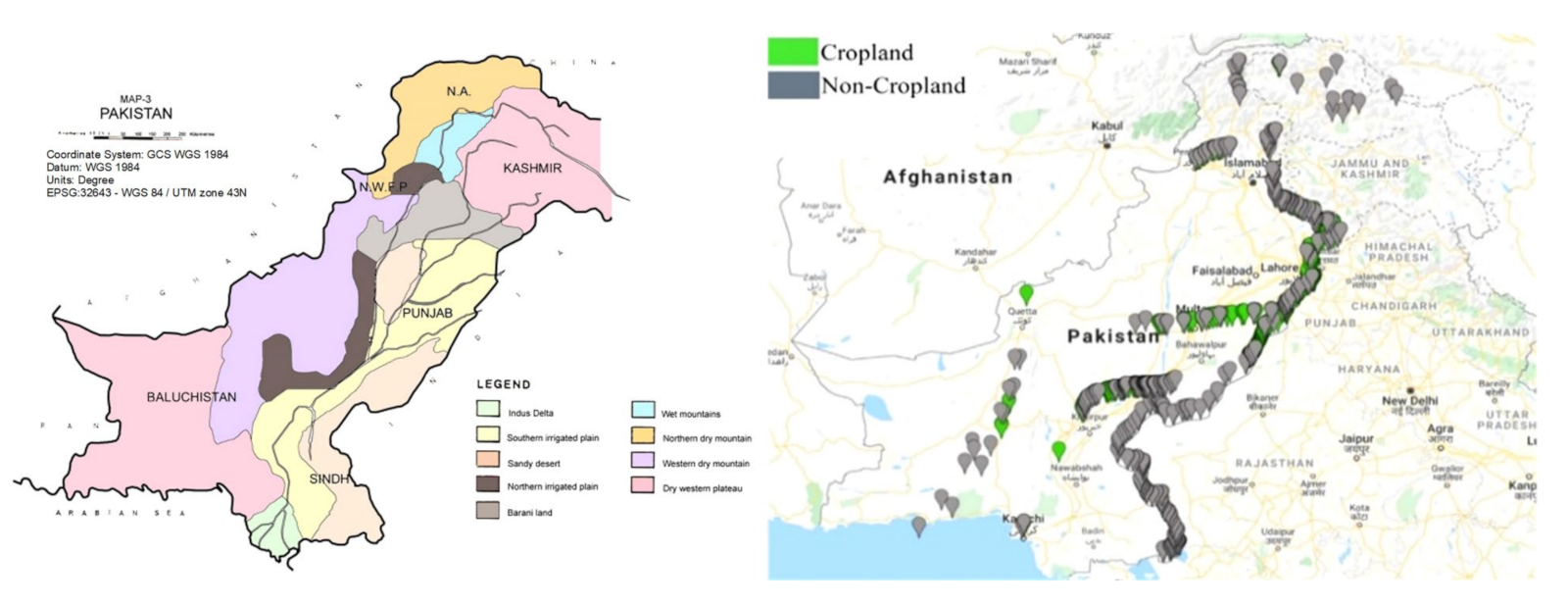
The literature uses various classification techniques and algorithms for picture segmentation and classification, including SVM, Deep Learning, Random Forest, and others. The Random Forest framework has been built with the help of particle swarm optimization and the learned representation of filter [67] photos of a road scene and an Indore scene in order to do semantic segmentation. Random Forest was used for landcover classification as an object-based image classification method [68]. The Mudrock picture segmentation model was built using deep learning and pixel values. A comparison was made between this model and the Random Forest algorithm to determine its efficacy [69]. Semantic ground cover segmentation in Worldview-2 pictures was performed using a CNN model. SVM and Random Forest were used to evaluate the outcomes [70]. Using the Semantic Texton Forest framework, we have successfully applied class-specific picture semantic segmentation based on textual and color characteristics to the publicly available datasets CamVid and MSRC-v2 [71]. Support Vector Machine (SVM) [72] has been implemented [73] to use landcover data to develop a unified method that can account for variations in both spectral and spatial dimensions. We examined the performance of four machine learning algorithms, Random Forest, Support Vector Machine, Naive Bayes, and k-Nearest Neighbor on satellite data for object-based analysis and semantic land cover segmentation [74]. Using optical remote sensing images, semantic segmentation, and a Deep Convolutional Network, we were able to forecast potential landslide danger zones [75]. To create a land cover map, we utilized the SVM algorithm on images from the CORONA collection [76]. A method of categorization was presented for use in object-based picture analysis via a comparison of random forest and support vector machine (SVM) for wetland area categorization utilizing Deep Convolutional Neural Networks (DCNN) and Fully Convolutional Networks (FCN). The difference results from the additional time and effort spent on the computer and on additional training data [77]. To classify the land cover dataset, a Multi-Level Feature Aggregation Network was introduced to combine feature extraction with up-sampling [78]. One way to segment the Kalideos database remote sensing images into distinct study areas was to use object and pixel processing. Using a Multilayer Feed-Forward Neural Network (MLFFNN), we compared its performance to that of SVM and Maximum Likelihood Classification when segmenting images for semantic meaning (MLC) [79]. Wetlands were modelled using four classifiers (k-Nearest Neighbor, Random Forest, and Decision Tree). Classification accuracy was calculated by comparing these models to a hybrid model including ANN [80]. The semantic segmentation of roadways, shoulders, guardrails, ditches, fences, and boundaries was performed using PointNet and ANN [81]. Using CNN’s features together with various filters and multi-resolution segmentation, a technique was proposed for semantic segmentation of LiDAR data and high-resolution optical images [82].

These methods use pixel-wise semantic segmentation to label the area of interest. Satellite photos are complicated and challenging to segment because of the similarities in the texture of different regions. These algorithms extract the texture, patterns, and orientation of images to identify distinct areas. The literature does not reveal any studies focusing on mapping agricultural acreage and increasing agricultural output to the same extent. Our group mapped agricultural farmland using semantic segmentation results to identify cultivated and uncultivated areas. The weak regions might be used in agriculture and horticulture to distribute food better. Additionally, it helps pinpoint the yearly decline of farmland, which is a crucial indicator for environmental sustainability. Compared with deep learning algorithms, machine learning methods such as Random Forest, Support Vector Machine (SVM), Naive Bayes, and CART are more efficient regarding data amounts, computational complexity, and memory utilization.

3. Study Area

Pakistan, located in Southern Asia, has a total land area of over 790,000 km² and has a moderate climate. Some regions of the United States have dry or semi-arid climates, whereas others do not. Most of Pakistan’s arable land is located in the country’s southern and eastern regions rather than its northern and western ones. The appearance of the same crop growing in several locations might vary considerably [83]. Mountains (such as the Himalayas and Karakoram), plateaus, bare-rock regions, and deserts are a part of the varied landscape. Most northern and southwestern farmland fields are small because mountains, bare rocks, and deserts are poor locations to raise crops. There are extensive plains in the southeast, with densely populated agricultural areas running beside the Indus River [84].

Our field of research included Pakistan, the world’s largest cropland region. Four developed agro-ecological zones, which help to define areas with everyday cultivation activities, and forms with soil and environment trends, are stratified among Pakistan’s regions, as shown in Figure 1.

Pakistan’s long history of extensive and cautious farming has resulted in sophisticated agricultural practices, a diverse selection of crops, and a variety of croplands that can adjust to a broad range of environmental and topographical factors [85]. When these factors come into play, it becomes more challenging to acquire farmland. Cropland on the southeastern plains is uniform in shape, closely spaced, and widely dispersed. The southwest plateaus are dotted with towns and farmland. Terraces and fields strung out along valleys and rivers may also be seen in the northern mountain areas. Pakistan, as a “paradigmatic example of Asian agriculture, is characterized by a wealth of crop varieties, significant spatial differences in crops, intra-class variations of the same crop in different regions, and complex small-scale farming techniques, including crop rotation on the same plot during different seasons and intercropping”.

There is a great deal of work in farmland mapping utilizing earth observation data sets despite the limited availability of operational charts, for various reasons. Identifying plant types necessitates using fine-scale time-lapse images to establish the minute differences between crop phenology. Second, crops are unique landscape units that require an adequate spatial resolution to be resolved unambiguously [86], which is the standard technological compromise between time and geographical resolution for Earth observation satellites. For data sets with poor spatial resolution, duplicated imagery at a given location does not yield a high return quality. Moderate-resolution imaging spectrometer (MODIS) sensors with a worse spatial resolution, such as 250 m per 250 m, have wider swaths and greater repeat imaging frequencies, but are restricted to producing accurate surface estimates for small farm sizes [87].

Since its introduction in 2015, Sentinel-2 has been available in two unique versions: Sentinel-2A and Sentinel-2B. Three hundred and fifty photographs from the Sentinel-2 satellite were selected using the Google Earth Engine (GEE); they were collected between January 2018 and December 2019. High-resolution Google Earth remotely sensed images were utilized to provide visual interpretations of land cover categories, and the Google Earth Engine platform was used to generate 857 training sample points and 200 test sample points at random. Vegetable gardens were retrieved together with planted croplands, since their distinction could not be made while processing remotely sensed images. Furthermore, in this case, we are talking about adjustments to the Food and Agricultural Organization’s (FAO) Global Agro-Ecological Zones (GAEZs), with a spatial resolution of 10 km, with an eye on the increasing importance of days, soil, and land [88]. As many of these locations contain a negligible proportion of cropland relative to the rest of the nation, the GAEZs include various zones to partition croplands. Consequently, we refined GAEZ into Refined Agro-Ecological Zones (RAEZs) with the ASTER Global Digital Model 2 (GDEM V2) 30 m data slope generated from 30 m GDEM and cropland percentage data in one region, utilizing advanced space-based thermal emission and reflection radiometers (ASTER). Various RAEZs, based on the area’s significance for croplands, are merged into vast regions.

4. Dataset

Data was used for the analysis of Sentinel-2 MSI (Level-1C). First, the satellite sensor data will be identified and discussed, followed by comparison validation and training in Pakistan.

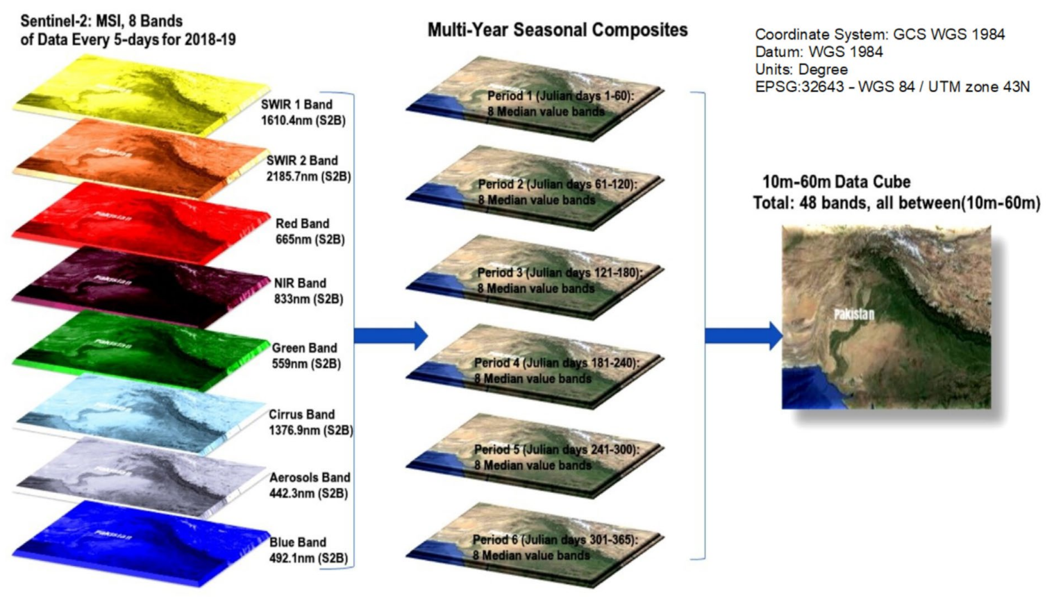
4.1. Sentinel-2 MSI Satellite Imagery Data

Data from the Sentinel-2 MSI satellite’s multi-spectral sensor were stored in Pakistan’s GEE cloud for two years (2018–2019) to study grain dynamics at different times of the year. Recent advances in multi-spectral sensors, such as the Sentinel-2 Multi-Spectral Imager (MSI), have improved signal-to-noise ratios and narrowed spectral bands, promising fruitful rangeland management [89]. According to research comparing S-2 to Landsat-8 and earlier Landsat sensors, the geographical and spectral ability of Sentinel-2 to differentiate between range and land management has been improved [90]. Information from Sentinel-2 between 10 m and 60 m in resolution is updated every 5 days. Due to cloud limitations, we cannot get continuous 5-day server-free time series results for wall-to-wall coverage over the whole region. Bimonthly composites were created to overcome this barrier and guarantee clear or almost perfect wall sight everywhere (taking into account the cloudiness of different countries and locations). As seen in Figure 2, mega-file data cubes (MFDCs) ranging in size from 10 m to 60 m were constructed. These MFDCs were used to generate a 48-band MFDC for six-time intervals (temporal composites).

Regarding the research region, we used the multi-year (2018–2019) five-day Sentinel-2 for (1) maintaining the wall-to-wall data coverage; and (2) maintaining the effect of the cloud coverage. Based on seasonal variations in the region and the quality of cloud-free Sentinel-2 data, the nominal years 2018 and 2019 were further subdivided into various cycles or phases. MFDC cloud-free wall-to-wall collections from Pakistan were developed in bi-monthly or tri-monthly intervals. The product of a total of six cycles (period 6: 301–365, period 5: 240–300, period 4: 181–240, period 3: 131–240, period 2: 61–120, and term 1: Julian 1–60 covering 12 months may be produced in cloud-free or nearly cloud-free pictures for bi-monthly intervals. Notably, Sentinel-2 multi-year (2018–2019) details are used to optimize the chances of cloud-free pixel purity over Pakistan over each period (e.g., 1–60 days). As a result, all Sentinel-2 five-day photographs were gathered covering Pakistan. Cirrus (1376.9 nm), Aerosol (442.3 nm), SWIR 2 (2185.7 nm), SWIR (1610.4 nm), NIR (833 nm), red (665 nm), green (559 nm), and blue (492.1 nm) were used with each duration. These images contributed to a 48-band MFDC with eight median-meaning bands consisting of six cycles. The band stack and periods lead to MFDC. Both compositions were carried out on the GEE cloud-based geospatial data research tool [43]. The restricted supply of temporal pictures and Sentinel-2 TOA items were used instead of Surface Reflectiveness (SR), as shown in Figure 2 and

Table 2. Sentinel 2: MSI 10 m to 60 m data used in the study characteristics multi-temporal multimedia.

	Name of the Data Provider	The Mega-File Data Cube with Total # of Bands	The Time-Composite of Julian Days over Data	Data Years	The Series of Sentinel-2	Name of the Data Provider
Pakistan	European Union/ESA/ Copernicus	48	C1: 1–60	2018, 2019	Multi-Spectral Instrument, Level-1C	European Union/ESA/ Copernicus
			C2: 61–120
			C3: 121–180
			C4: 181–240
			C5: 241–300
			C6: 301–365

.

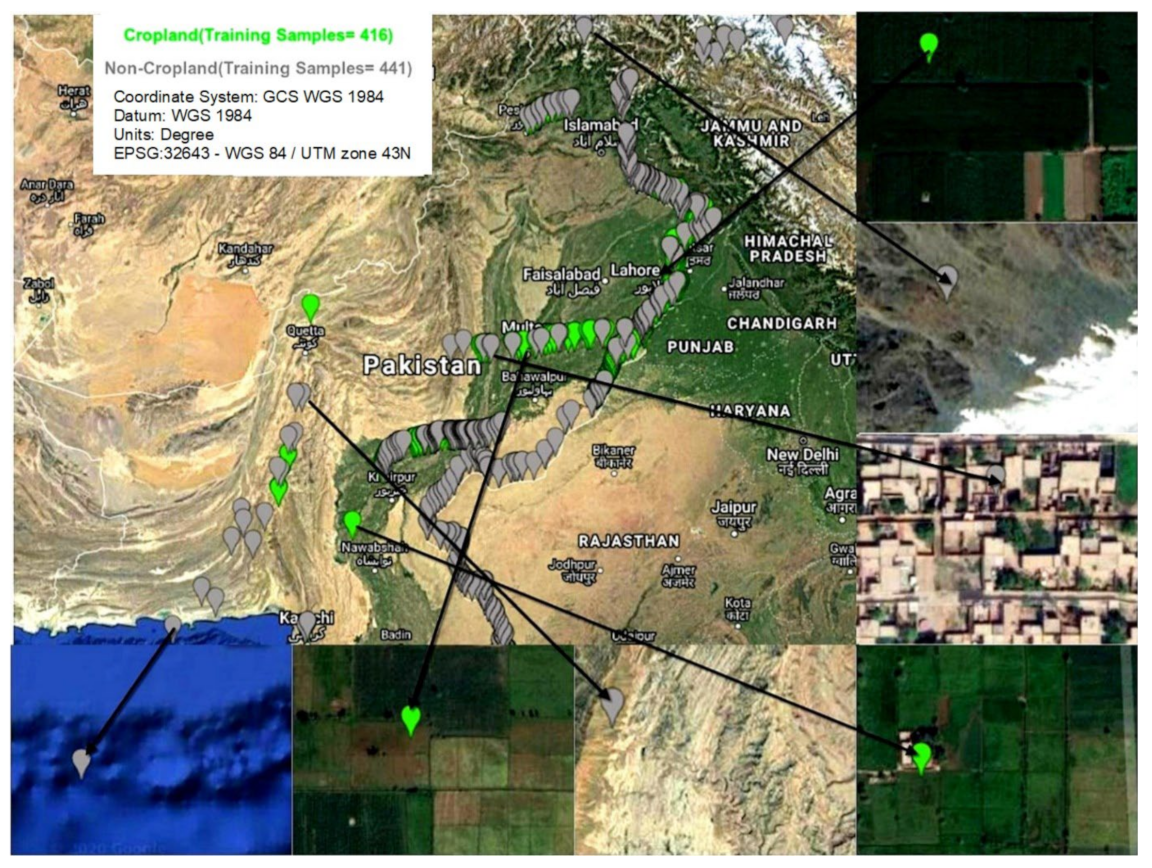
4.2. Training and Validation Sample Croplands

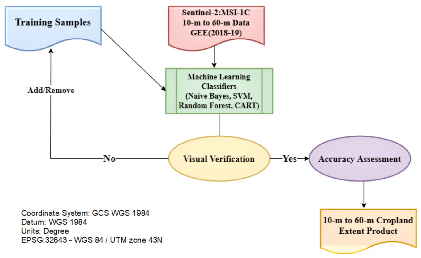
In the following stage, Pakistan’s training and assessment data were compiled. Training and testing data points or samples have been collected to train our machine learning algorithms in this phase. A machine learning algorithm used training samples to learn the underlying knowledge and then used these samples as a reference for classifying the land surface as cropland or non-cropland areas. Furthermore, testing samples were used to test how well our machine learning algorithm learned from the training phase. Samples have been obtained for a wide range of cropland and non-cropland groups with stable distribution in Pakistan. Validation data have been used for precision, mistake, and uncertainty. Croplands have been described as farmlands with an annual crop standing + croplands fallows + permanent crops [21]. The comparison training and evaluation data were then correctly labeled. In Pakistan, other observations were made using very high spatial resolution imaging (VHRI) sub-meter to 10-m and several years of Google Earth Engine photos. Of these, 857 measurements and 200 study samples were obtained, as shown in Figure 3.

Table 3. Education and confirmation details on sources. A collection of comparison samples used by machine-learning algorithms and the number of testing samples required to determine autonomous accuracy.

	Class	Training Samples	Validation Samples
Pakistan	Cropland	416	100
	Non-Cropland	441	100

describes the distribution of the comparison training and validation results.

5. Methodology

The objective of the analysis was for Pakistan to develop the correct cropland scale commodity Sentinel-2 at 10 m to 60 m. Figure 3 illustrates the procedure to generate croplands for Pakistan utilizing five days’ time-series data for the 2018–2019 time frame. We have implemented a pixel-based supervised classification technique using the many machine learning classifiers in the GEE cloud computing architecture. A description of the method has been provided in Figure 4.

5.1. Machine Learning Algorithms

We have selected four different algorithms: Rides, Support Vector Machine (SVM), Random Tree, and Naïve Bayes Pixel-based supervised. In addition, the algorithm accuracies listed were compared. They are often robust to detect noise and overfitting and are particularly effective for categorizing remote sensing devices. In remote sensing systems, SVM receives the most attention. SVMs are subjected to highly effective classifiers and possible remote sensing data inquiry methods. SVMs have a technique for categorization, not a statistical norm but a geometrical norm based on the margins. To achieve the categorization function, SVMs do not require inferences of statistical distribution in the groups, but by manipulating the edge maximization model, they describe the categorizing model [91]. An array of binary decision trees constructs a random forest classifier by selecting a portion of the sample bootstrap from the input data and selecting an informative subset for each partition [92]. The RF concept is superior to that of a single decision tree. The bootstrap combines (bag) a collection of decision trees by scanning random subspaces from the data (features) and breaking up the nodes at most, eliminating the association between the trees. In random forest, graders often quantitatively calculate the contribution of each variable to the classification performance, which is helpful in determining the significance of each variable. They have a test of internal precision for an ‘off-bag’ technique (OOB), in which roughly one third of the knowledge is retained as a test data collection to determine the classification accuracy. The RF classification can be cross-validated using separate data sets. The GEE ran specific forest classifiers using five inputs: (1) classification tree numbers, (2) leaf maxes, (3) decision tree input percentage, (4) out-of-bag mode of the random seed variable, and (5) the decision tree development random seed variable. The random forest classification variable in GEE requires six input parameters. With growing numbers of plants, the average classification accuracy improves non-excessively [93].

The Naive Bayes Method is a Bayesian classification methodology that predicts a class mark for a data instance by the distribution of attribute values, and is a statistical and linear classification method. It is a parametric classification in which the assignment element remains consistent. The distribution of the nucleus, multivariate or multi-nominal, can be the usual (Gaussian). Bayesian classifiers use the theorem of Bayes to determine subsequent probabilities for all class input results. The data instance [94] is allocated to class labels with optimum conditional probability. These distribution assumptions would influence the creation of the NBC model and model parameters. If an attribute defined to an entity is identified by $\mathrm{F}=\left\{{\mathrm{f}}_1,\dots ,{\mathrm{f}}_{\mathrm{d}}\right\}$, and the distribution of each attribute (function) is natural, then the probability (process), recognized as a class j^th(Cj), is as the following equation:

$$\mathrm{P}(\mathrm{F}|{\mathrm{C}}_{\mathrm{j}})={\displaystyle \prod _{k=1}^{d}P({\mathrm{F}}_{\mathrm{k}}|{\mathrm{C}}_{\mathrm{j}})}={\displaystyle \prod _{k=1}^d\mathrm{N}({\mathrm{f}}_{\mathrm{k}};{\hat{\mu }}_{\mathrm{j}\mathrm{k}};{\hat{\sigma }}_{\mathrm{j}\mathrm{k}})}$$

(1)

where ${\hat{\mu }}_{\mathrm{j}\mathrm{k}}$ and ${\hat{\sigma }}_{\mathrm{j}\mathrm{k}}$ are estimated results of μ and σ for the k^th feature and j^th class. Then, by using the conditional probability rule, the following equation is obtained.

$$\mathrm{P}({\mathrm{C}}_{\mathrm{j}}|\mathrm{F})=\mathrm{P}({\mathrm{C}}_{\mathrm{j}})\mathrm{P}(\mathrm{F}|{\mathrm{C}}_{\mathrm{j}})=\mathrm{P}({\mathrm{C}}_{\mathrm{j}}){\displaystyle \prod _{k=1}^d\mathrm{N}({\mathrm{f}}_{\mathrm{k}};{\hat{\mu }}_{\mathrm{j}\mathrm{k}};{\hat{\sigma }}_{\mathrm{j}\mathrm{k}})}$$

(2)

The description outcomes of the artifacts may be calculated based on their attributes (functions) with the maximum probability value of P (${\mathrm{C}}_{\mathrm{j}}$|F)

$$\hat{c}={\arg }_{{\mathrm{c}}_{\mathrm{j}}}\max \mathrm{P}({\mathrm{C}}_{\mathrm{j}}){\displaystyle \prod _{k=1}^d\mathrm{N}({\mathrm{f}}_{\mathrm{k}};{\hat{\mu }}_{\mathrm{j}\mathrm{k}};{\hat{\sigma }}_{\mathrm{j}\mathrm{k}})}$$

(3)

where ${\mathrm{C}}_{\mathrm{j}}$ is the description of the outcome/output.

The CART is a supervised computer analysis algorithm that constitutes a binary decision tree, similar to the Decision Tree algorithm. It necessitates defining and developing the tree using samples for which the optimal classification cannot be determined. The Decision Tree concludes with a root node for each element in the function space, minimizing the uncleanness of all nodes. The decision tree then progresses through incremental splits, so impurity does not decrease dramatically as more separation is introduced [95]. Therefore, the decision tree expands. The tree of judgment consists of multi-level and multi-leaf nodes, and after it has been built, the judgment tree is broken. The designed trees are sometimes unnecessarily suited because there is always a disproportionate number of knots and branches. The tree may be sliced by manipulating the younger branches’ parameters or thresholds.

The following procedures were used to train machine-learning algorithms to construct an iterative sample selection process to achieve an appropriate sample size, as shown in Figure 5. The step-by-step approach is listed below:

• Produce a computer description of current examples in instruction.
• Classify MFDC from 10 m to 60 m based on the existing classification with the GEE cloud on Support Vector Machine, Random Forest, and Naïve Bayes algorithms, as shown in Figure 2.
• Visually examine the categorization tests using current reference maps and sub-meter to 10-m VHRI.
• Connect field samples to designated zones with comparison submeter to 10 m VHRI from Google Earth Imagery.
• Repeat measures 1–4 of the expanded training data collection to optimize classification and obtain high precision.

The number of iterations available for the sample collection of the testing depends on the area’s difficulty. To conduct the classification shown in Figure 3, Pakistan has been divided into many agro-ecological regions (see Figure 1), with the iterative sorting frequently replicated ∼2–3 fold, enhancing the initial categorized performance. We began with a limited number of samples (250 to begin with) and then gradually increased the measurement size to a high degree of precision. Following each repetition, we visually contrasted the classification outcome at 100 s of locations with submeters of VHRI of 10 m. When the assessment outcomes were insufficient, we passed the tests sufficiently. Using the independent validation results, the accuracy evaluation team conducted accuracy analysis, as shown in Table 3.

5.2. Google Earth Platforms Cloud Computing

For the pixel description of croplands, we have used Google Earth Engine (GEE) cloud computing for machine learning algorithms. GEE’s accessible Sentinel-2 MSI archives are already optimized for atmospheric and topographical impacts, saving us much time in accessing the information. Throughout the GEE application editor, we used the JavaScript API. Google Fusion tables were utilized to import all testing samples and zonal boundaries into GEE (Appendix A).

Remote Sensing Analysis Accuracy on the GEE Platform

GEE generally performed exceptionally in simplifying access to remote sensing products through the cloud platform and executing sophisticated processes for satellite data processing. Numerous processed-ready satellite scenes or composites are immediately available to the user. Even though our research did not focus on massive volumes of data, we demonstrated that the GEE cloud platform might be used to construct massive-scale applications that access and analyze satellite data. Because of what GEE can do, the methods discussed in the paper can be used globally. The study also looked at the validity or accuracy of crop mapping with GEE using existing commodities and processing chains.

However, we think that there are a few things that need to be changed before GEE can be used to map crops on a large scale, especially in an operational context:

• It would help if it was possible to find solutions to the problem of data loss caused by weather conditions (such as clouds and shadows) that were easily accessible.
• Improve existing classifiers, especially the SVM, by incorporating neural network classifiers (through a library such as TensorFlow’s deep learning capabilities).

6. Results and Discussion

This portion consists of three distinct components, beginning with a demonstration of the ML-based mapping technique for Pakistan using up to 60 m of Sentinel-2 MSI, followed by an evaluation of farmland distribution precision, errors, and uncertainties. Finally, croplands are described and addressed at a regional level.

Having accurate, detailed, and high-resolution farmland maps at the national scale is crucial for ensuring long-term agricultural productivity and food security [96]. This research looked at the feasibility of using a machine-learning-based method to precisely map and label GEE’s agricultural districts. Other authors have indicated that the GEE cloud platform provides a legitimate tool and processing environment for generating a precise and accurate cropland extent product in a matter of minutes [97] thanks to its computing capacity and well-integrated large-scale analytic approaches.

As a result of its unusual revisit frequency of 5 days (for twin satellites S2A and S2B) and 10m per pixel spatial resolution, Sentinel-2 was chosen as the significant resource satellite to identify and map agricultural distribution at the field size. Since fields and farms in Pakistan and similar locations are, on average, 0.9 hectares in size and only data with such high spatial resolution can give sufficient information for efficient and detailed crop monitoring and classification, Sentinel-2 is better suited to the diversity of agroecosystems, terrain patterns, and agricultural methods present there.

Our approach is premised on extracting phenological variables (metrics) for farmland-type mapping, since these characteristics have previously shown their usefulness in monitoring and identifying unique vegetation cover at different spatial scales [98].

Moreover, the findings confirmed the efficacy of the machine learning techniques used in GEE to create granular estimates of agricultural expansion over large regions. Classifiers from the field of machine learning (Support Vector Machine, CART, Naive Bayes, and Random Forest) were chosen because they produce probabilities for each label, are computationally efficient when dealing with large amounts of data, have outperformed other state-of-the-art methods, and have few parameters that need tuning [54]. Since complex classification will involve more uncertainty when numerous classes concurrently occupy the same pixel [99], this final benefit gives a soft category (probability estimate), which is especially relevant in Pakistan’s fragmented and diversified landscapes. The probability maps we generate are well correlated with the corresponding high-resolution images. Each pixel was classified as cropland or non-cropland based on the probability maps, and the threshold used was 60%. These findings represent a significant improvement above the state-of-the-art, as seen in Figure 5. The standard picture stacking approach, which may miss critical phenological events and make it impossible to identify the farmland or crop type, has been replaced by our suggested framework, which incorporates phenological data to map cropland and how it varies. Furthermore, current products prioritize LULC even when the primary objective is not to create a comprehensive map of agricultural areas. Moreover, they are exclusively accessible for specific years and are seldom updated [100].

Some additional difficulties arise when using GEE to locate reference samples in areas with insufficient ground data. When operating in Asia, obtaining a representative sample at the Sentinel scale and choosing a uniform pixel is challenging. The only way to solve this issue is to improve the quality of the input samples, include more data layers whenever feasible, and do away with the outliner altogether. Using Google Earth Engine to locate reference samples raises eyebrows, since the resulting interpretations are not as reliable as data gathered in the field. Previous studies, however, corroborate the usefulness of rapid and easy methods of mapping land cover. Crowdsourced Google Earth data regarding the geographical distribution of farmland in Pakistan was found to be more accurate than global land cover datasets. People tend to understate the extent to which humans affect things when analyzing crowdsourced data, and there was little difference between specialists and non-experts in terms of identifying human impact.

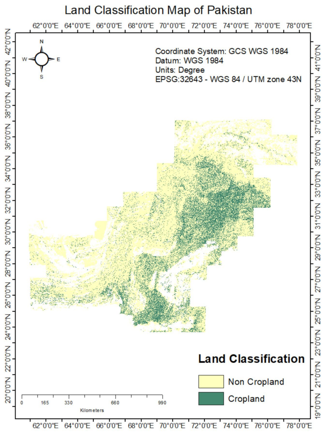
6.1. 10 m to 60 m Cropland Extent Product for Pakistan

In the nominal years 2018–2019, the trial generated 10 m to 60 m of croplands extracted from Sentinel-2 MSI 5-day time series data for Pakistan. The machine learning algorithms listed in Section 4 were used to distinguish croplands from non-croplands in the GEE cloud computing setting. The method was iterated, and the samples were modified and input to the algorithms several times before optimum cultivable cropland outcomes relative to non-cropland were obtained (see Figure 5).

6.2. Accuracy Assessment

The cropland map for Pakistan was evaluated for accuracy with an error matrix that did not apply to the manufacturer of this dataset [101]. The accuracy error matrix has been developed for the entire world. The precision of the ultimate cropland map of Pakistan was calculated using a minimum of 200 stratified, randomly spaced testing samples. An error matrix, as shown in

Table 4. The computer analysis performance error matrix algorithms. The 10 m to 60 m cropland expanded commodity for Pakistan’s precision error matrix.

CART Algorithm Accuracy on Training and Validation Datasets
	Cropland	Non-Cropland	Total	User Accuracy	Classification Accuracy: 93% Validation Accuracy: 82%
Cropland	73	27	100	73%
Non-Cropland	9	91	100	91%
Total	82	118	200
Producer Accuracy	89%	77%
Random Forest Algorithm Accuracy on Training and Validation Datasets
	Cropland	Non-Cropland	Total	User Accuracy	Classification Accuracy: 91% Validation Accuracy: 75%
Cropland	71	29	100	71%
Non-Cropland	21	79	100	79%
Total	92	108	200
Producer Accuracy	77%	73%
Naïve Bayes Algorithm Accuracy on Training and Validation Datasets
	Cropland	Non-Cropland	Total	User Accuracy	Classification Accuracy: 83% Validation Accuracy: 76%
Cropland	54	46	100	54%
Non-Cropland	13	87	100	87%
Total	67	133	200
Producer Accuracy	81%	65%
Support Vector Machine Algorithm Accuracy on Training and Validation Datasets
	Cropland	Non-Cropland	Total	User Accuracy	Classification Accuracy: 83% Validation Accuracy: 74%
Cropland	68	32	100	68%
Non-Cropland	21	79	100	79%
Total	89	111	200
Producer Accuracy	76%	71%

for complete accuracy (Pakistan as a whole), Naïve Bayes, Ride, Random Tree, and SVM algorithms was developed, and its accuracy on a 10 m to 60 m Sentinel-2 MSI dataset and validation data collection is provided below. In the validation dataset, the average precision of the CART algorithm was 82%, with an accuracy of 89% for the producer and 73.0% for the customer for the cropland class. The validation data collection had a complete accuracy of 75% for the Random Forest method, a vendor accuracy of 77% for the cropland class, and an implementation accuracy of 71.0%. The validation data collection was 76% for the Naïve Bays method, 81% for the manufacture, and 54.0% for the cropland class for consumer accuracy. Similarly, SVM’s total validity data accuracy was 74%, the producer’s accuracy was 76%, and cropland accuracy was 68%. Table 4 demonstrates the performance of the algorithm CART with the best average validity performance relative to the other three algorithms. Classification accuracy defines the performance of the machine learning algorithm on the provided training data, while validation accuracy defines the implementation of the machine learning algorithm on detailed testing data supplied to the algorithm externally.

Classification accuracies can be further increased, particularly the accuracies of the consumer and supplier (see Table 4), by separating the regions (see Figure 1). Google Earth Engine (GEE) is a powerful tool for capturing, storing and classifying photographs via a cloud storage network. While GEE allows the handling of extensive data and easy calculations, it is restricted to how GEE handles comprehensive data using MLAs. There are still several obstacles to overcome, such as the lack of data on comparative training from agricultural fields of greater variety. By illustration, for a specific classifier, the study of the entire broad data population contributes to inconsistencies in the classification performance and a decrease in accuracy instead of classifying data for each pixel. Many directions to boost precision and raise uncertainty are better than spatial mappings, such as the convergence of global forest maps [102] and global water masks [103]. Since 10 m to 60 m of Sentinel-2 images include thousands of pixels in such broad fields, this is not a substantial study, but is perhaps the best one to obtain, considering the difficulty of general areas and capital. Larger samples for training and testing are possible, particularly in numerous croplands, including highland to lowland deltas that consider specific subspecies within permanent cultivations, cropland falls, and permanent plants. Similar approaches have often been implemented in many nations of the world in addition to those employed here. In a recent report on Africa [56], for instance, 94% of the development lands had an average weighted precision (85% or 14.1% omission error) and 68.5% (31.5% commission error), with a producers’ accuracy of 85%, and an Africa overall consumer accuracy of 31.5% (commission error).

6.3. The Analogy to Other Datasets and Agricultural Regions

Aside from creating a map, it is an essential component of the 10 m to 60 m region of cropland commodity to quantify the cropland region statistics. Pakistan features two distinct types of croplands (croplands and pastures under management). For 2018–2019, Pakistan’s gross cropland region was estimated to have been 370,200 square kilometers.

Table 5. Net cropland areas derived based on the 10 m to 60 m Sentinel-2 MSI.

Country.	Agriculture Land in Sq. Km (The World Bank Data)	Govt. of Pakistan (Agriculture Census Organization-2010) in Sq. Km.	Net Cropland Area in Sq. Km. (Estimated in the Current Study)	Agriculture Land (Pakistan Bureau of Statistics) in Sq. Km.	% of the Total Agriculture Land Areas
Pakistan	368,440	274,814	370,200	303,400	47.79%

presents statistics for the cropland area produced for Pakistan in this study compared to other sources like the Pakistan Statistical Bureau. However, the area created by this analysis of the cultivated land in Pakistan between 10 m and 60 m is high. Every pixel up to 60 m is approximately 0.099 ha. It is, therefore, necessary, also at the farm stage, vast or small-scale, to catch regions at the sub-national level. It is a significant advantage in contrast to other current cropland goods.

6.4. Input Parameters for Cropland Extent Mapping

After examining the literature and conducting tests, we decided to use nine bands for this analysis: green, red, blue, SWIR1, SWIR2, and near-infrared, as well as the vegetation indices EVI, NDVI, and LSWI (see

Table 6. Characteristics of Sentinel 2 MSI data used in this study.

Band Name	Sentinel 2-MSI Wavelength (nm)	Vegetation Index (VI)	Equation
Blue	496.6 nm (S2A)/492.1 nm (S2B)	EVI	EVI = 2.5 (NIR-red)/(NIR + 6*red–7.5*blue + 1)
Green	560 nm (S2A)/559 nm (S2B)
Red	664.5 nm (S2A)/665 nm (S2B)	NDWI	NDWI = (NIR-SWIR1)/(NIR + SWIR1)
NIR	835.1 nm (S2A)/833 nm (S2B)
SWIR1	1613.7 nm (S2A)/1610.4 nm (S2B)
SWIR2	2202.4 nm (S2A)/2185.7 nm (S2B)	NDVI	NDVI = (NIR-red)/(NIR + red)

). NDVI was used to detect dense plant groupings, such as forests. The Enhanced Vegetation Index (EVI) is a modified version of the Normalized Difference Vegetation Index (NDVI) that was created to detect plants that were too faintly luminous to be seen with the naked eye. The cultivable land was determined using the Normalized Difference Water Index (NDWI). The USGS formerly performed Top of Atmosphere (TOA) processing before the images were used: when this study was undertaken for Sentinel-2 on GEE, insufficient Surface Reflectance images were available. In addition, we have chosen to incorporate GDEM-derived elevation, which helps machine learning classifiers differentiate between classes with similar spectral signatures but different characteristics. It is especially beneficial for separating rice fields in river deltas and other low-lying agricultural regions from higher-lying agricultural and non-crop areas in the uplands. Combining ground data with sub-meter to 5-m data and supplementary data based on their relative elevation permits the identification of several spectrally-related groups.

7. Conclusions

Using Sentinel-2 data for the notional years 2018–2014, this research created the first map of Pakistan’s farmland expanse at a resolution of 60 m. This research used the Google Earth Engine to showcase the efficacy of pixel-based CART, Random Forest, Naive Bayes, and Support Vector machine learning algorithms for agricultural farmland mapping across extensive regions, with a resolution of 60 m. (GEE). The CART algorithm has the best validation accuracy (82%) among the various machine learning techniques. Table 4 displays the detailed accuracy evaluation analysis and confusion matrix for Pakistan’s 60 m Landsat-derived agricultural extent product for 2018–2019. The research team used “48 input bands derived from seasonal composites of remotely sensed observations, topographic variables, 857 reference training samples, and 200 reference validation samples spread across 14 Agro-Ecological zones to develop a novel approach to creating cropland versus non-cropland maps”. According to the agricultural map, the study area has 370,200 square kilometers of cropland, or 47.79% of Pakistan’s total agricultural land.

Considering the “computer capacity and ever-expanding archive of satellite observation accessible in GEE, the classification technique used in this work may be duplicated to map net croplands for additional years in the same study regions, as well as in any other location and period given the inputs”. Research into environmental monitoring, climate change, land cover change, land use, food security, water, agriculture, and policy development all stand to benefit significantly from the findings given here.

8. Future Work

Large-scale optical and SAR crop mapping considers the worldwide coverage of the Landsat-8, Proba-V, Sentinel-1, and Sentinel-2 satellites. We want to implement a parcel-based classification approach based on the GEE-linked pixel method, in addition toother methods, to improve the pixel-based crop classification map.

References

1. Estévez, J.; Salinero-Delgado, M.; Berger, K.; Pipia, L.; Rivera-Caicedo, J.P.; Wocher, M.; Reyes-Muñoz, P.; Tagliabue, G.; Boschetti, M.; Verrelst, J. Gaussian processes retrieval of crop traits in Google Earth Engine based on Sentinel-2 top-of-atmosphere data. Remote Sens. Environ. 2022, 273, 112958. [Google Scholar] [CrossRef]
2. Suni, T.; Guenther, A.; Hansson, H.C.; Kulmala, M.; Andreae, M.O.; Arneth, A.; Artaxo, P.; Blyth, E.; Brus, M.; Ganzeveld, L.; et al. The significance of land-atmosphere interactions in the Earth system—iLEAPS achievements and perspectives. Anthropocene 2015, 12, 69–84. [Google Scholar] [CrossRef] [Green Version]
3. Lutter, S.; Pfister, S.; Giljum, S.; Wieland, H.; Mutel, C. Spatially explicit assessment of water embodied in European trade: A product-level multi-regional input-output analysis. Glob. Environ. Chang. 2016, 38, 171–182. [Google Scholar] [CrossRef] [Green Version]
4. van Zanten, H.H.; Mollenhorst, H.; Klootwijk, C.W.; van Middelaar, C.E.; de Boer, I.J. Global food supply: Land use efficiency of livestock systems. Int. J. Life Cycle Assess. 2016, 21, 747–758. [Google Scholar] [CrossRef] [Green Version]
5. Pfister, S.; Vionnet, S.; Levova, T.; Humbert, S. Ecoinvent 3: Assessing water use in LCA and facilitating water footprinting. Int. J. Life Cycle Assess. 2016, 21, 1349–1360. [Google Scholar] [CrossRef]
6. Davis, K.F.; Rulli, M.C.; Seveso, A.; D’Odorico, P. Increased food production and reduced water use through optimized crop distribution. Nat. Geosci. 2017, 10, 919–924. [Google Scholar] [CrossRef]
7. Waldner, F.; Canto, G.S.; Defourny, P. Automated annual cropland mapping using knowledge-based temporal features. ISPRS J. Photogramm. Remote Sens. 2015, 110, 1–13. [Google Scholar] [CrossRef]
8. Gumma, M.K.; Thenkabail, P.S.; Maunahan, A.; Islam, S.; Nelson, A. Mapping seasonal rice cropland extent and area in the high cropping intensity environment of Bangladesh using MODIS 500 m data for the year 2010. ISPRS J. Photogramm. Remote Sens. 2014, 91, 98–113. [Google Scholar] [CrossRef]
9. Estel, S.; Kuemmerle, T.; Alcántara, C.; Levers, C.; Prishchepov, A.; Hostert, P. Mapping farmland abandonment and recultivation across Europe using MODIS NDVI time series. Remote Sens. Environ. 2015, 163, 312–325. [Google Scholar] [CrossRef]
10. Shao, Y.; Lunetta, R.S.; Ediriwickrema, J.; Iiames, J. Mapping cropland and major crop types across the Great Lakes Basin using MODIS-NDVI data. Photogramm. Eng. Remote Sens. 2010, 76, 73–84. [Google Scholar] [CrossRef] [Green Version]
11. Shao, Y.; Lunetta, R.S. Sub-pixel mapping of tree canopy, impervious surfaces, and cropland in the Laurentian Great Lakes Basin using MODIS time-series data. IEEE J. Sel. Top. Appl. Earth Obs. Remote Sens. 2010, 4, 336–347. [Google Scholar] [CrossRef]
12. He, Y.; Lee, E.; Warner, T.A. A time series of annual land use and land cover maps of China from 1982 to 2013 generated using AVHRR GIMMS NDVI3g data. Remote Sens. Environ. 2017, 199, 201–217. [Google Scholar] [CrossRef]
13. Pittman, K.; Hansen, M.C.; Becker-Reshef, I.; Potapov, P.V.; Justice, C.O. Estimating global cropland extent with multi-year MODIS data. Remote Sens. 2010, 2, 1844–1863. [Google Scholar] [CrossRef] [Green Version]
14. Thenkabail, P. Global Food Security Support Analysis Data at Nominal 1 km (GFSAD1km) Derived from Remote Sensing in Support of Food Security in the Twenty-First Century: Current Achievements and Future Possibilities. In Land Resources Monitoring, Modeling, and Mapping with Remote Sensing; CRC Press: Boca Raton, FL, USA, 2018; pp. 865–894. [Google Scholar]
15. Liang, D.; Zuo, Y.; Huang, L.; Zhao, J.; Teng, L.; Yang, F. Evaluation of the consistency of MODIS Land Cover Product (MCD12Q1) based on Chinese 30 m GlobeLand30 datasets: A case study in Anhui Province, China. ISPRS Int. J. Geo-Inf. 2015, 4, 2519–2541. [Google Scholar] [CrossRef] [Green Version]
16. Ran, Y.; Li, X. First comprehensive fine-resolution global land cover map in the world from China—Comments on global land cover map at 30-m resolution. Sci. China Earth Sci. 2015, 58, 1677. [Google Scholar] [CrossRef]
17. Arsanjani, J.J.; Tayyebi, A.; Vaz, E. GlobeLand30 as an alternative fine-scale global land cover map: Challenges, possibilities, and implications for developing countries. Habitat Int. 2016, 55, 25–31. [Google Scholar] [CrossRef]
18. Yang, Y.; Xiao, P.; Feng, X.; Li, H. Accuracy assessment of seven global land cover datasets over China. ISPRS J. Photogramm. Remote Sens. 2017, 125, 156–173. [Google Scholar] [CrossRef]
19. Chen, Z.; Zhao, S. Automatic monitoring of surface water dynamics using Sentinel-1 and Sentinel-2 data with Google Earth Engine. Int. J. Appl. Earth Obs. Geoinf. 2022, 113, 103010. [Google Scholar] [CrossRef]
20. Belgiu, M.; Csillik, O. Sentinel-2 cropland mapping using pixel-based and object-based time-weighted dynamic time warping analysis. Remote Sens. Environ. 2018, 204, 509–523. [Google Scholar] [CrossRef]
21. Gumma, M.K.; Thenkabail, P.S.; Deevi, K.C.; Mohammed, I.A.; Teluguntla, P.; Oliphant, A.; Xiong, J.; Aye, T.; Whitbread, A.M. Mapping cropland fallow areas in myanmar to scale up sustainable intensification of pulse crops in the farming system. GIScience Remote Sens. 2018, 55, 926–949. [Google Scholar] [CrossRef]
22. Vogels, M.F.; de Jong, S.M.; Sterk, G.; Addink, E.A. Agricultural cropland mapping using black-and-white aerial photography, object-based image analysis and random forests. Int. J. Appl. Earth Obs. Geoinf. 2017, 54, 114–123. [Google Scholar] [CrossRef]
23. Löw, F.; Prishchepov, A.V.; Waldner, F.; Dubovyk, O.; Akramkhanov, A.; Biradar, C.; Lamers, J.P. Mapping cropland abandonment in the Aral Sea Basin with MODIS time series. Remote Sens. 2018, 10, 159. [Google Scholar] [CrossRef] [Green Version]
24. Liu, J.; Zhu, W.; Cui, X. A shape-matching cropping index (CI) mapping method to determine agricultural cropland intensities in China using MODIS time-series data. Photogramm. Eng. Remote Sens. 2012, 78, 829–837. [Google Scholar] [CrossRef]
25. Biradar, C.M.; Thenkabail, P.; Turral, H.; Noojipady, P.; Jie, L.Y.; Velpuri, M.; Dheeravath, V.; Venkateswarlu, V.; Vithanage, J.; Jagath, L.; et al. A global map of rainfed cropland areas (GMRCA) at the end of last millennium using remote sensing. Int. J. Appl. Earth Obs. Geoinf. 2009, 11, 114–129. [Google Scholar] [CrossRef]
26. Nellis, M.D.; Price, K.P.; Rundquist, D. Remote sensing of cropland agriculture. In The SAGE Handbook of Remote Sensing; SAGE Publications, Inc.: New York, NY, USA, 2009; Volume 1, pp. 368–380. [Google Scholar]
27. Sweeney, S.; Ruseva, T.; Estes, L.; Evans, T. Mapping cropland in smallholder-dominated savannas: Integrating remote sensing techniques and probabilistic modeling. Remote Sens. 2015, 7, 15295–15317. [Google Scholar] [CrossRef] [Green Version]
28. Oliphant, A.J.; Thenkabail, P.S.; Teluguntla, P.; Xiong, J.; Gumma, M.K.; Congalton, R.G.; Yadav, K. Mapping cropland extent of Southeast and Northeast Asia using multi-year time-series Landsat 30-m data using a random forest classifier on the Google Earth Engine Cloud. Int. J. Appl. Earth Obs. Geoinf. 2019, 81, 110–124. [Google Scholar] [CrossRef]
29. Alberto, R.; Serrano, S.C.; Damian, G.B.; Camaso, E.E.; Celestino, A.B.; Hernando, P.J.C.; Isip, M.F.; Orge, K.M.; Quinto, M.J.C.; Tagaca, R.C.; et al. Object Based Agricultural Land Cover Classification Map of Shadowed Areas from Aerial Image and Lidar Data Using Support Vector Machine. In Proceedings of the 2016 ISPRS Congress, Prague, Czech Republic, 12–19 July 2016; Volume 3. [Google Scholar]
30. Sitthi, A.; Nagai, M.; Dailey, M.; Ninsawat, S. Exploring land use and land cover of geotagged social-sensing images using naive bayes classifier. Sustainability 2016, 8, 921. [Google Scholar] [CrossRef] [Green Version]
31. Xiong, J.; Thenkabail, P.S.; Gumma, M.K.; Teluguntla, P.; Poehnelt, J.; Congalton, R.G.; Yadav, K.; Thau, D. Automated cropland mapping of continental Africa using Google Earth Engine cloud computing. ISPRS J. Photogramm. Remote Sens. 2017, 126, 225–244. [Google Scholar] [CrossRef] [Green Version]
32. Friesz, A.M.; Wylie, B.K.; Howard, D.M. Temporal expansion of annual crop classification layers for the CONUS using the C5 decision tree classifier. Remote Sens. Lett. 2017, 8, 389–398. [Google Scholar] [CrossRef]
33. Teluguntla, P.; Thenkabail, P.S.; Xiong, J.; Gumma, M.K.; Congalton, R.G.; Oliphant, A.; Poehnelt, J.; Yadav, K.; Rao, M.; Massey, R. Spectral matching techniques (SMTs) and automated cropland classification algorithms (ACCAs) for mapping croplands of Australia using MODIS 250-m time-series (2000–2015) data. Int. J. Digit. Earth 2017, 10, 944–977. [Google Scholar] [CrossRef] [Green Version]
34. Teluguntla, P.; Thenkabail, P.S.; Xiong, J.; Gumma, M.K.; Congalton, R.G.; Oliphant, J.A.; Sankey, T.; Poehnelt, J.; Yadav, K.; Massey, R.; et al. NASA Making Earth System Data Records for Use in Research Environments (MEaSUREs) Global Food Security-support Analysis Data (GFSAD) Cropland Extent 2015 Australia, New Zealand, China, Mongolia 30 m V001. 2017. Available online: http://oar.icrisat.org/10980/ (accessed on 5 December 2022).
35. Zhong, L.; Hu, L.; Yu, L.; Gong, P.; Biging, G.S. Automated mapping of soybean and corn using phenology. ISPRS J. Photogramm. Remote Sens. 2016, 119, 151–164. [Google Scholar] [CrossRef] [Green Version]
36. Bellón, B.; Bégué, A.; Lo Seen, D.; De Almeida, C.A.; Simões, M. A remote sensing approach for regional-scale mapping of agricultural land-use systems based on NDVI time series. Remote Sens. 2017, 9, 600. [Google Scholar] [CrossRef] [Green Version]
37. Xie, Y.; Lark, T.J.; Brown, J.F.; Gibbs, H.K. Mapping irrigated cropland extent across the conterminous United States at 30 m resolution using a semi-automatic training approach on Google Earth Engine. ISPRS J. Photogramm. Remote Sening. 2019, 155, 136–149. [Google Scholar] [CrossRef]
38. Useya, J.; Chen, S.; Murefu, M. Cropland Mapping and Change Detection: Toward Zimbabwean Cropland Inventory. IEEE Access 2019, 7, 53603–53620. [Google Scholar] [CrossRef]
39. Del Valle, T.M. Comparison of common classification strategies for large-scale vegetation mapping over the Google Earth Engine platform. Int. J. Appl. Earth Obs. Geoinf. 2022, 115, 103092. [Google Scholar] [CrossRef]
40. Quang, N.H.; Nguyen, M.N.; Paget, M.; Anstee, J.; Viet, N.D.; Nones, M.; Tuan, V.A. Assessment of Human-Induced Effects on Sea/Brackish Water Chlorophyll-a Concentration in Ha Long Bay of Vietnam with Google Earth Engine. Remote Sens. 2022, 14, 4822. [Google Scholar] [CrossRef]
41. Onačillová, K.; Gallay, M.; Paluba, D.; Péliová, A.; Tokarčík, O.; Laubertová, D. Combining Landsat 8 and Sentinel-2 Data in Google Earth Engine to Derive Higher Resolution Land Surface Temperature Maps in Urban Environment. Remote Sens. 2022, 14, 4076. [Google Scholar] [CrossRef]
42. Erickson, T. Multi-Source Geospatial Data Analysis with Google Earth Engine; American Geophysical Union (AGU): Fall Meeting Abstracts, Washington, DC, USA, 2014. [Google Scholar]
43. Gorelick, N.; Hancher, M.; Dixon, M.; Ilyushchenko, S.; Thau, D.; Moore, R. Google Earth Engine: Planetary-scale geospatial analysis for everyone. Remote Sens. Environ. 2017, 202, 18–27. [Google Scholar] [CrossRef]
44. Praticò, S.; Solano, F.; Di Fazio, S.; Modica, G. Machine learning classification of mediterranean forest habitats in google earth engine based on seasonal sentinel-2 time-series and input image composition optimisation. Remote Sens. 2021, 13, 586. [Google Scholar] [CrossRef]
45. Seydi, S.T.; Akhoondzadeh, M.; Amani, M.; Mahdavi, S. Wildfire damage assessment over Australia using sentinel-2 imagery and MODIS land cover product within the google earth engine cloud platform. Remote Sens. 2021, 13, 220. [Google Scholar] [CrossRef]
46. Sun, Y.; Qin, Q.; Ren, H.; Zhang, Y. Decameter Cropland LAI/FPAR Estimation from Sentinel-2 Imagery Using Google Earth Engine. IEEE Trans. Geosci. Remote Sens. 2021, 60, 1–14. [Google Scholar] [CrossRef]
47. Ahmad, D.; Chani, M.I.; Humayon, A.A. Major crops forecasting area, production and yield evidence from agriculture sector of Pakistan. Sarhad J. Agric. 2017, 33, 385–396. [Google Scholar] [CrossRef]
48. Yan, L.; Roy, D.P.; Li, Z.; Zhang, H.K.; Huang, H. Sentinel-2A multi-temporal misregistration characterization and an orbit-based sub-pixel registration methodology. Remote Sens. Environ. 2018, 215, 495–506. [Google Scholar] [CrossRef]
49. Li, J.; Roy, D.P. A global analysis of Sentinel-2A, Sentinel-2B and Landsat-8 data revisit intervals and implications for terrestrial monitoring. Remote Sens. 2017, 9, 902. [Google Scholar] [CrossRef] [Green Version]
50. FAO. Pakistan: Review of the Wheat Sector and Grain Storage; Food and Agriculture Organization: Rome, Italy, 2013. [Google Scholar]
51. Pakistan Bureau of Statistics. Agricultural Census 2010—Pakistan Report; Pakistan Bureau of Statistics: Islamabad, Pakistan, 2010. [Google Scholar]
52. Basso, B.; Cammarano, D.; Carfagna, E. Review of crop yield forecasting methods and early warning systems. In Proceedings of the First Meeting of the Scientific Advisory Committee of the Global Strategy to Improve Agricultural and Rural Statistics, Rome, Italy, 18 July 2013. [Google Scholar]
53. Boryan, C.; Yang, Z.; Mueller, R.; Craig, M. Monitoring US agriculture: The US department of agriculture, national agricultural statistics service, cropland data layer program. Geocarto Int. 2011, 26, 341–358. [Google Scholar] [CrossRef]
54. Pelletier, C.; Webb, G.I.; Petitjean, F.J.R.S. Temporal convolutional neural network for the classification of satellite image time series. Remote Sens. 2019, 11, 523. [Google Scholar] [CrossRef] [Green Version]
55. Pelletier, C.; Valero, S.; Inglada, J.; Champion, N.; Dedieu, G. Assessing the robustness of Random Forests to map land cover with high resolution satellite image time series over large areas. Remote Sens. Environ. 2016, 187, 156–168. [Google Scholar] [CrossRef]