Article

Using Stable Sulfur Isotope to Trace Sulfur Oxidation Pathways during the Winter of 2017–2019 in Tianjin, North China

Institute of Surface-Earth System Science, School of Earth System Science, Tianjin University, Tianjin 300072, China
*
Author to whom correspondence should be addressed.
Int. J. Environ. Res. Public Health 2022, 19(17), 10966; https://doi.org/10.3390/ijerph191710966
Submission received: 26 July 2022 / Revised: 27 August 2022 / Accepted: 29 August 2022 / Published: 2 September 2022

Abstract

:
After the implementation of the Coal Replacing Project (CRP) in the northern parts of China in 2017, its effect on PM2.5 composition is still unclear. In the study, water-soluble ionic components (WSICs) and stable sulfur isotope ratios (δ34S) of SO42− in PM2.5 collected during the domestic heating period before and after the implementation of CRP in Tianjin were analyzed. Results showed that the average concentrations of both PM2.5 and WSICs have dropped dramatically after the CRP, especially for the SO42− (by approximately 57–60%). After the CRP, the range of δ34Ssulfate was significantly narrowed to 4.1–7.5‰ in January 2018 and 1.4–6.1‰ in January 2019, which suggested that the sulfur source was becoming simple. It was interesting that the δ34Ssulfate value in the pollution period before the CRP was higher than that in the clean period, whereas it showed the opposite tendency after the CRP, which implied that the contribution of sea salt was high during the pollution period before the CRP. The MIXSIAR model calculated that the contributions of the transition-metal ion (TMI) oxidation and NO2 oxidation pathways in the three sampling stages were higher than those of the OH radical oxidation and H2O2/O3 oxidation pathways, indicating that the formation pathway of sulfate was mainly dominated by heterogeneous oxidation. Before the CRP, the NO2 oxidation pathway was the dominant sulfate oxidation pathway during a haze episode, and the TMI oxidation pathway dominated the formation of sulfates after the CRP.

1. Introduction

In recent years, many urban areas in China have been severely affected by haze [1,2,3]. The primary emissions, secondary formation and transformation, and stable weather conditions have been considered as the main reasons for such widespread and continuous high loading of air pollutants, including haze, over China [4,5,6]. During certain special events, the Chinese government adopted some temporary policies to pursue a great improvement in air quality, such as shutting down heavily polluting industries, prohibiting construction activities, and reducing the number of vehicles in operation [7,8]. However, the impact of these measures was limited, and the improvement in air quality could not be maintained for a long time [7,9,10]. Among many control measures taken during the “Action Plan on Prevention and Control of Air Pollution” since 2013, the Coal Replacing Project (CRP), i.e., the consumption of electricity and natural gas instead of coal for energy, was an important solution for the Chinese government to achieve the goal of reducing fine particulate matter (PM2.5) permanently.
It has been widely reported that the CRP has significant impacts on the energy, the economy, and the environment domains [11,12,13]. Lin and Jia (2020) concluded that the main significance of the coal-to-electricity project was not saving energy but improving air quality [12]. Ren et al. (2017) reported that the contributions of coal combustion to n-alkanes, PAHs, and OPAHs in Urumqi have been decreased from 21~75% before the implementation of CRP to 4.0~21% after the CRP [14]. Feng et al. (2020) found that the contribution of coal combustion to nitrate in the winter has been decreased by about 8% compared to the implementation of the CRP in Tianjin, and the amount of nitrate produced by the heterogeneous formation pathway has been reported to be increased after the implementation of the CRP [7]. However, most of the recent studies have focused on the role of the CRP in the emission reduction of pollutants (such as PM2.5, SO2, and NOx) [15,16], yet the impact of the CRP on the changes in source contributions and composition of particulate matter could not be adequately evaluated.
As a major component of PM2.5, the sulfate concentrations generally increase rapidly due to haze [17]. Previously, fossil fuel combustion was considered the main source of sulfate in the atmosphere [18], especially from coal burning. Although the energy structure has been changed by the CRP, fossil fuels were still the main energy composition and sulfates still played an important role. Therefore, studies on the formation mechanism of sulfate before and after the CRP could help to better evaluate the environmental effects of the CRP. Moreover, the δ34S sulfate could provide the oxidation pathways of SO2 in the atmosphere [19,20], and it has been utilized for identifying the formation pathways in haze episodes by analyzing the δ34S of sulfate [21,22]. Over 90% of sulfate in haze episodes was secondary sulfate and sulfate produced from SO2 oxidation in the atmosphere via (1) gas-phase oxidation by OH radical [23,24]; (2) aqueous oxidation by H2O2, O3, and transition-metal ion (TMI)-catalyzed O2 [25]; and (3) heterogeneous oxidation on the surface of aerosols, cloud droplets, and mineral dust by the same oxidants as aqueous oxidation [26]. Some studies also suggested that the conversion of SO2 to sulfate could be promoted by the coexistence of NOx [17,20,25], especially during haze [24,27,28].
This study was based on the response of water-soluble ionic components (WSICs) and δ34Ssulfate in PM2.5 before and after the implementation of the CRP in the year from 2017 to 2019. The variation of pollution characteristics of WSICs, δ34Ssulfate, and oxidation pathways of sulfate were studied to ascertain the impact of CRP on the formation of PM2.5 in the polluted periods. Furthermore, the improvement of air pollution due to coal-to-electricity and coal-to-natural gas policies could also be better evaluated.

2. Materials and Method

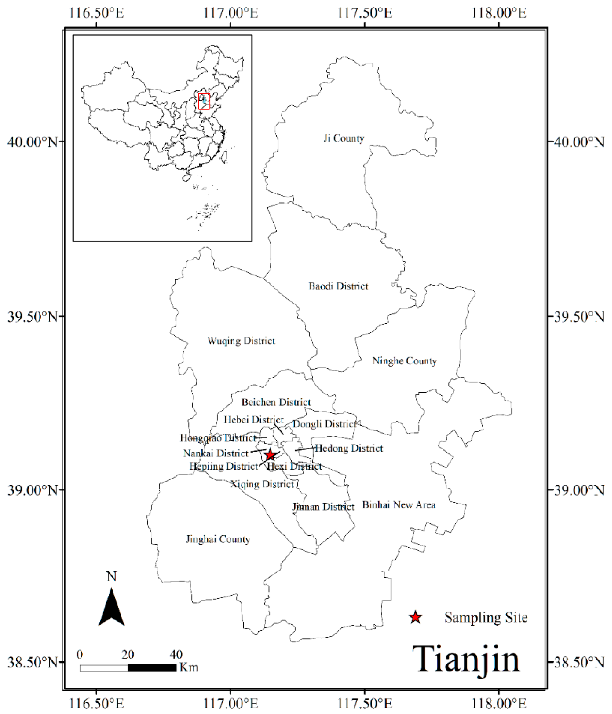
2.1. Sample Collection

PM2.5 sampling was conducted on the rooftop (~25 m high) of a 6-storey teaching building in Tianjin University, located at 39.11° N, 117.16° E in the center of Tianjin, which represents a typical urban environment (Figure 1) during the winter (domestic heating period) of three consecutive years, i.e., 2017, 2018, and 2019 (Table S1). PM2.5 samples collection membranes were pre-combusted when collected (450 °C for 6 h). Quartz filters (23 × 18 cm) using a high-volume air sampler (TE-PM2.5HVP-BL, TISCH, Cleves, OH, USA) at a flow rate of 1.05 m3 min−1 during 8:00–18:00 (local time) for daytime and from 18:00 to next morning 8:00 for nighttime in both the seasons, and stored at −20 °C. The membranes were weighed before and after sampling using a microelectronic balance (Mettler Toledo ML 204T, Switzerland) after a 48-h equilibration in a drying vessel. One blank filter was also collected in each campaign. The samples were classified into clean (PM2.5 ≤ 75 μg m−3) and polluted (PM2.5 > 75 μg m−3) periods based on the PM2.5 mass concentration. Temperature (T), relative humidity (RH), and wind speed (WS) were measured at sampling points using a meteorological station (Gill MetPak, Gill Instruments, Lymington, Hampshire, UK). Gaseous pollutant (O3, SO2 and NO2) concentrations collected from the Tianjin Air Quality Monitoring Station data, located 1.7 km away from the sampling site.

2.2. Chemical Composition Analysis

Two filter cuts with a diameter of 44 mm (or four filter cuts of 26 mm in diameter if the PM2.5 concentration was low) were used for the analysis of WSICs. The filters were extracted into 15 mL ultrapure water (18.2 MΩ cm, Millipore, Burlington, MA, USA) under ultrasonication for 30 min at room temperature. The extractants were filtered through a 0.22 μm PTFE membrane filter and then the ions were measured using ion chromatography (ICS-5000+, Thermal, Sunnyvale, CA, USA). Cations were measured using a Dionex IonPacTM CS12A analytical column and a Dionex CRDS 600 suppressor on a conduction detector, and 20 mM MSA was used as an eluent. At a flow rate of 1.0 mL min−1 for anion measurement, 30 mM KOH was used as an eluent with a Dionex IonPacTM AS11-HC RFIC TM analytical column. The detection limit for WSICs was lower than 2 ng mL−1 with an error < 5%.

2.3. Determination of Sulfur Isotopic (δ34S) Ratios

Half of each quartz fiber filter was cut into pieces for δ34S analysis. They were extracted into 50 mL of ultrapure water and sonicated for 15 min, and then repeated three times. The solution was then filtered with 0.45 μm syringe filters. The filtrate was acidified to a pH < 2 by adding HCl solution and then trapped as barium sulfate (BaSO4) by adding droplets of supersaturated BaCl2 solution. The BaSO4 precipitation was filtered using 0.22 μm acetate filters 24 h later. After heating in an oven with step-wise heating at 200 °C for 2 h, 400 °C for 2 h, and 850 °C for 4 h, 340–450 μg BaSO4 were weighted and wrapped in tin capsules. The tin cups were crushed into a small size and placed into the isotope ratio mass spectrometer (MAT253, Thermo, Waltham, MA, USA). The δ34S of BaSO4 was standardized with laboratory barite standards (referenced to NBS-127 and IAEA SO-5), and reported to the international sulfur isotope standard V-CDT [22].
The δ34S of SO42− was calculated by Equation (1):
δ34Ssulfate = [(34S/32S)sample/(34S/32S)standard − 1] × 1000
where the isotopic ratio of (34S/32S)standard = 0.044. Overall uncertainty for δ34Ssulfate values reported here were ±0.2‰ [22].

2.4. MIXSIAR Model to Calculate the Formation Pathways of Sulfate Aerosols

In this estimation, isotope fractionation effects from SO2 to SO42− have to be considered. Many previous studies have shown that the fractionation factors of δ34S from SO2 to SO42− depend on the extent of the reaction [24,29]. Moreover, the isotope fractionation factor between SO2 and SO42− could be calculated by the Rayleigh distillation model, which was based on an instantaneous phase equilibrium process under an open system (Rayleigh 1896). In the model, the δ34S value of SO2 is a function of δ34Semission, the fraction:
δ34SSO2 = δ34Semission + ɛobs × ln(1 − SOR)
where δ34SSO2 is the δ34S of remaining SO2 in the atmosphere; ɛobs is the fractionation factor between SO2 and SO42−; SOR is the SO2 oxidation ratio; δ34Semission is the δ34S of SO2 in emission sources, which can be estimated by the following formula based on the isotope mass balance [21]:
δ34Semission = δ34SSO2 × (1 − SOR) + δ34Ssulfate × SOR
where δ34Ssulfate is the δ34S value of observed SO42− in the atmosphere. When SOR is close to 1, δ34Semission equals to δ34Ssulfate. Assuming the emitted SO2 is completely converted to sulfate (SOR = 1), δ34Semission is calculated according to the linear relationship between δ34Ssulfate and SOR in each sampling stage. According to the Equations (2) and (3), the fractionation factor (ɛobs) can be calculated:
ɛobs = (δ34Semission − δ34Ssulfate) × SOR/[(1 − SOR) × ln(1 − SOR)]
Using the observed δ34Ssulfate, SOR, and the estimated δ34Semission, we found the mean values of ɛobs during the sampling period were 6.6 ± 2.2‰, 0.6 ± 1.1‰, −3.1 ± 0.4‰ and 4.2 ± 1.1 ‰ during January 2017, July 2017, January 2018, and January 2019, respectively. The difference in ɛobs values reflected the different formation mechanisms of sulfate aerosols. The oxidation pathways of sulfate mainly involve gas-phase oxidation and aqueous-phase reactions [23,24,25]. Several laboratory experiments measured the fractionation factors (ɛ) for SO2 oxidation through H2O2 and O3, and these two pathways showed similar ɛ values ranging from +15.1‰ to +17.4‰ [28]. Therefore, we used ɛH2O2/O3 to represent the combined isotopic effect of O3 and H2O2 pathways. The fractionation factors (ɛ) for SO2 oxidation through OH radical, H2O2/O3, NO2, and TMI pathways can be calculated [28]:
ɛOH (‰) = − (0.004 ± 0.015) × T + (10.60 ± 0.73)
ɛH2O2/O3 (‰) = − (0.085 ± 0.004) × T + (16.51 ± 0.15)
ɛTMI (‰) = − (0.237 ± 0.004) × T + (−5.039 ± 0.044)
lnɛNO2 (‰) = (0.2437 ± 0.0457)/T − (0.0008 ± 0.019)
where T is the ambient temperature (°C). Based on the observed temperature in Tianjin during the sampling period, the fractionation factors of different oxidation pathways were obtained. Instead, the εobs should be a result of the mixing of multiple oxidation pathways [21]:
ɛobs = ɛOH × fOH + ɛH2O2/O3 × fH2O2/O3 + ɛTMI × fTMI + ɛNO2 × fNO2
where fi is the contribution of oxidation pathway i to sulfate formation, and fOH + fH2O2/O3 + fTMI + fNO2 = 1. Based on Equation (8), a Bayesian isotope mixing model (ran in the Stable Isotope Analysis in the R, MIXSIAR) was used to assess the contributions of oxidation pathways to sulfate. A logical prior distribution was established in this model first, and the contribution of each oxidation pathway to the mixture was then determined.

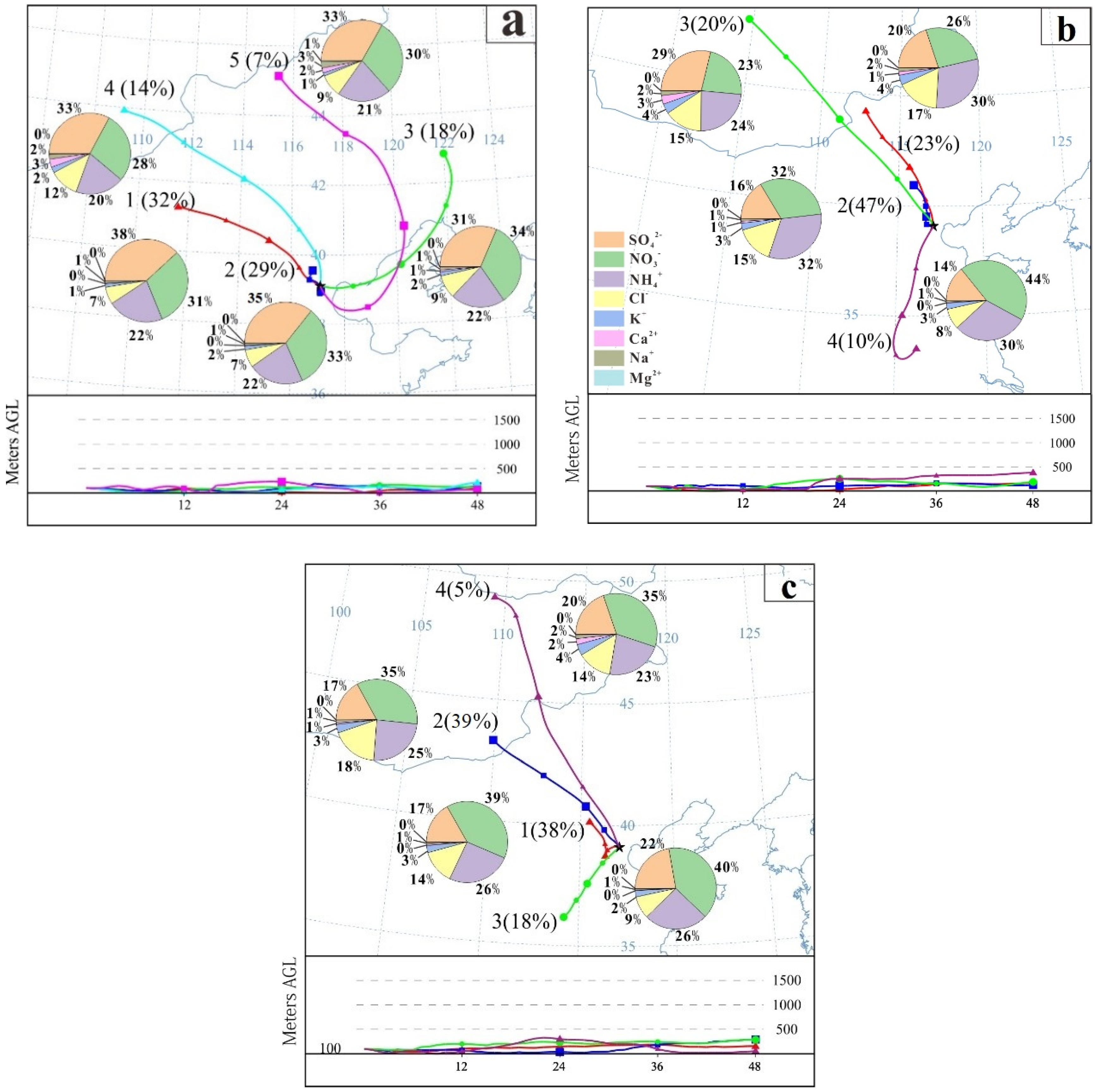
2.5. HYSPLIT Backward Trajectory Analysis

This study mainly used the Hybrid Single Particle Lagrangian Integrated Trajectory Model (HYSPLIT4) of the MeteoInfo software to analyze the trajectory of backward gas and backward air mass. In this study, 100 m was regarded as the average flow field height of atmospheric boundary layer, and the backward trajectory of air mass movement is simulated every 48 h. Combined with the Pearson correlation analysis of sulfur and RH, T, SOR, tried to clarify the main factors affecting the change of S concentration in PM2.5.

2.6. Boundary Layer Height (BLH) Simulation

In order to explore the influence of BLH change on PM2.5 pollution in Tianjin during the pollution period, the study was conducted in the region of 116.75° to 118° east longitude and 38.5° to 39.5° north latitude, including most of Tianjin and a small part of Bohai Sea. The study area consisted of 30 grids (one grid corresponds to one height value), the resolution is 0.25° × 0.25° (about 27 km × 27 km), and the BLH per hour was obtained by connecting 30 grids (height value) together. The Data from “The Climate Data Store” (https://cds.climate.copernicus.eu/cdsapp#!/home, accessed on 5 May 2022).

3. Results and Discussion

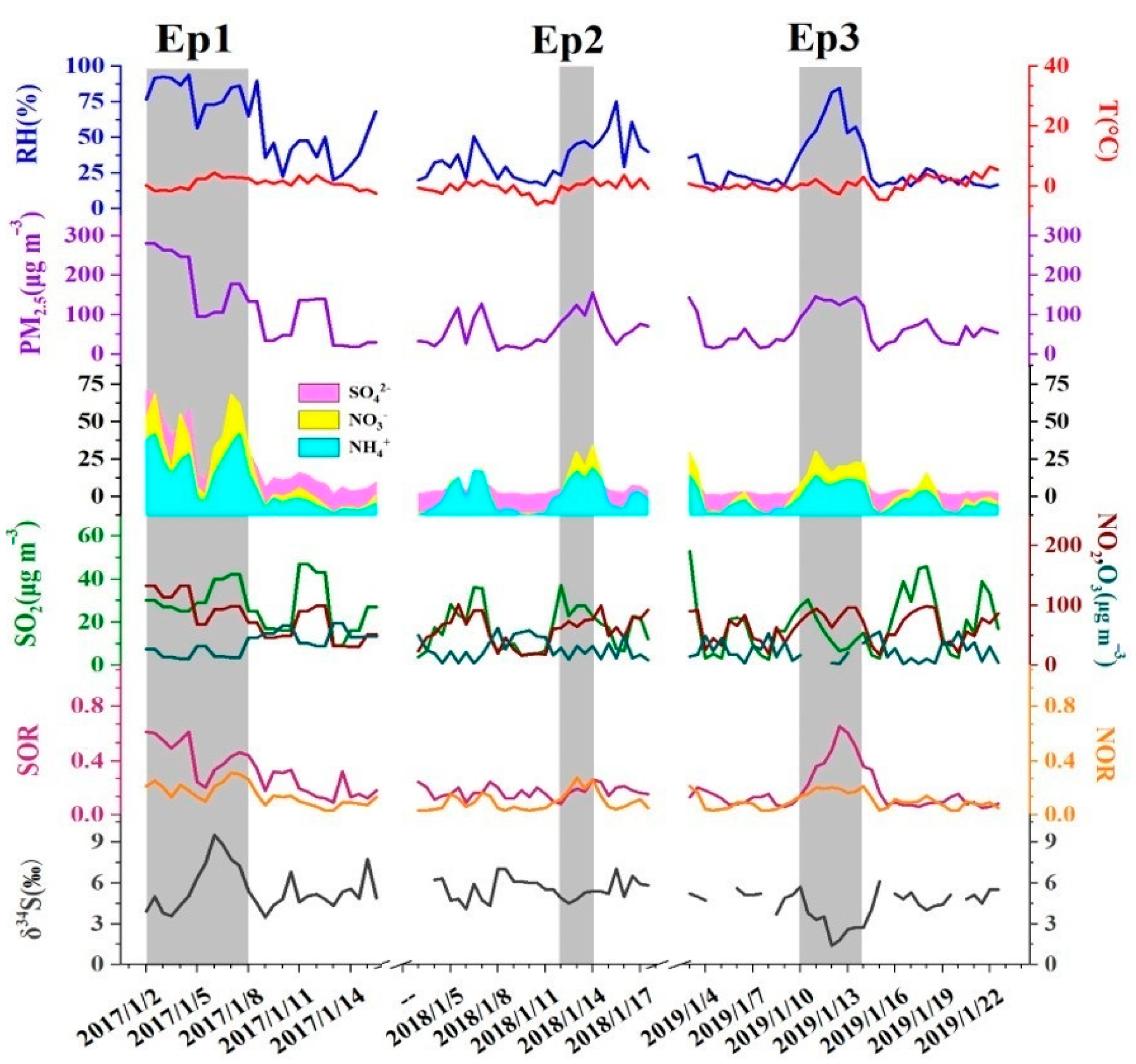
3.1. Effect of CRP on PM2.5 Loading and Its Composition

As summarized in Table 1, the average concentration of PM2.5 in January 2018 and January 2019 dropped by approximately 60% and 57%, respectively, compared to that in January 2017. In addition, the mean value of boundary layer height (BLH) in 2017 was 313 m, which was close to 300 m in 2019 (Figure S1), indicating a great improvement in air quality after the implementation of CRP in Tianjin. In the winter of three years, three typical haze episodes (Ep1, Ep2 and Ep3) during sampling were discussed in Section 3.3.
However, the PM2.5 concentration two years after the implementation of CRP (January 2019) was slightly higher than that one year after the implementation of the project (January 2018), and the SO2 and NO2 concentrations in the atmosphere also showed similar annual changes (Table 1). In addition, the RH and WS were similar in January 2018 and January 2019 (Table 1). We speculated that, first, BLH in 2019 (300 m) was much smaller than that in 2018 (524 m), which makes it difficult to diffuse pollutants (Figure S1). Secondly, we assumed that in the first year of the implementation of CRP, the “coal-to-gas” and “coal-to-electricity” transformation projects were implemented strictly, and the amount of coal consumption was greatly reduced, resulting in a very low PM2.5 concentration in January 2018. Whereas in the second year of the CRP, some areas have the situation that the natural gas supply was not enough to support the heating demand and the consumption of coal was partly resumed to supplement the natural gas, and the coal consumption in January 2019 was slightly higher than that in January 2018 (Figure S2), which should be one of the main reasons for causing the increased PM2.5 loading in January 2019 compared to that in January 2018.
As shown in Figure 2, sulfate, nitrate, and ammonium (SNA) were the most important three components of WSICs, and the variation of SNA was consistent with the PM2.5 concentrations. The concentration of SNA in January 2017 was higher than that in January 2018 and January 2019. Otherwise, as shown in Figure S3, the proportion of sulfate in SNA decreased, and the proportion of nitrate and ammonium in SNA increased after the CRP was implemented.

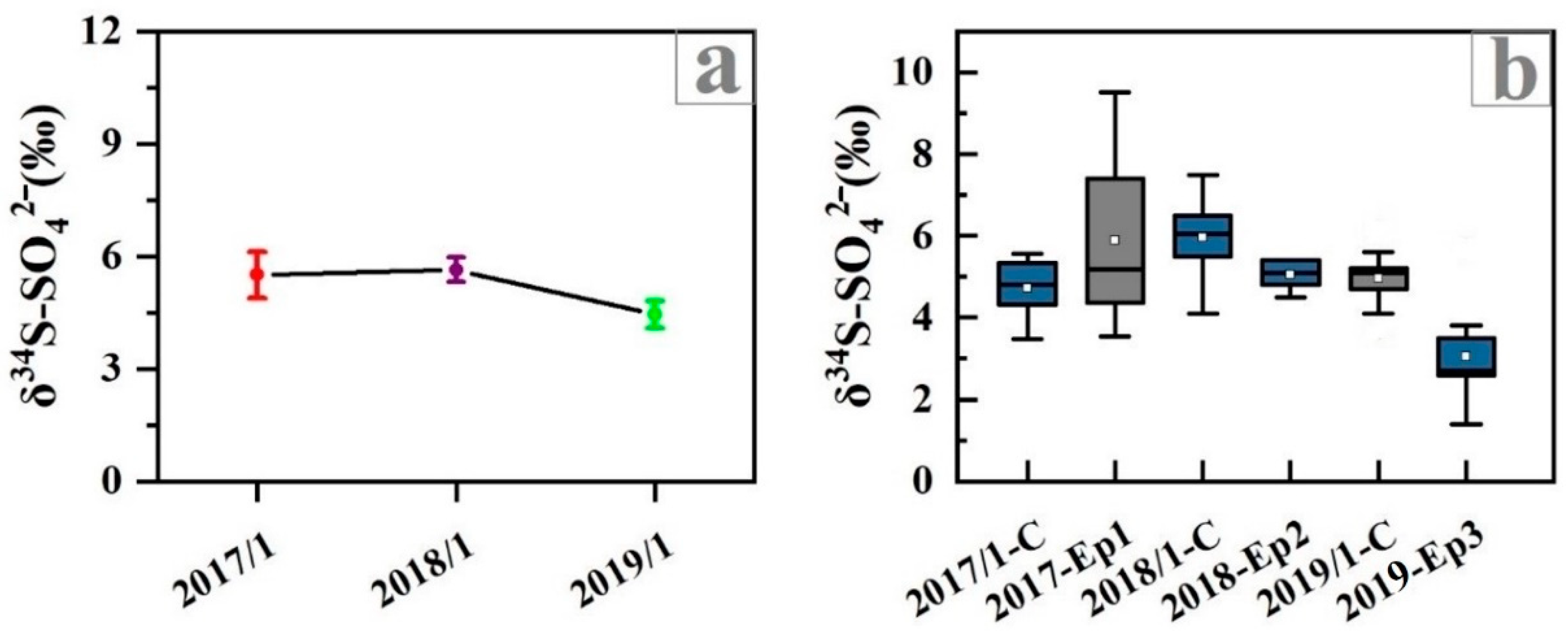
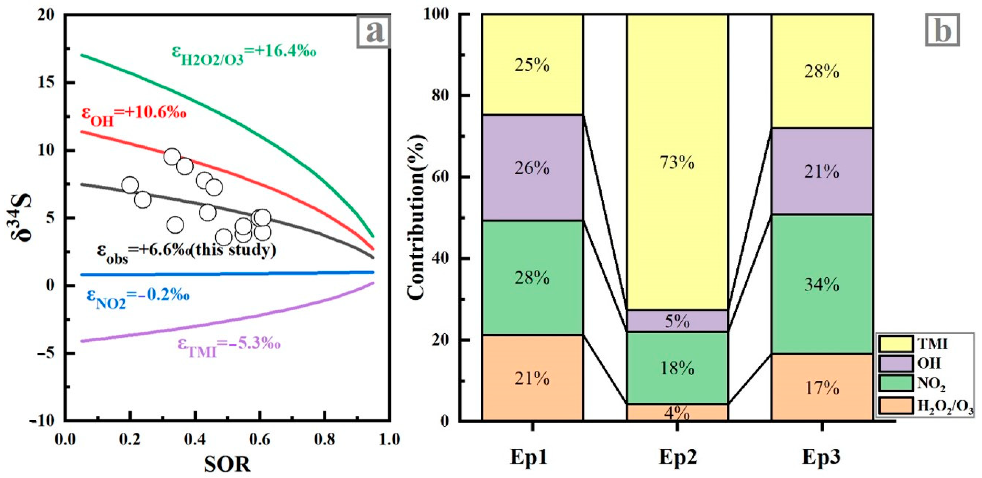
3.2. Sulfur Isotope Composition of Sulfate Aerosols

As shown in Figure 3, before the implementation of the CRP (January-2017), the δ34Ssulfate varied widely from 3.5 to 9.5‰ with a mean value of 5.5 ± 1.6‰, and the range of δ34Ssulfate was narrowed after the CRP was implemented, which were 4.1~7.5‰ in January 2018 with a mean value of 5.6 ± 0.9‰, and 1.4~6.1‰ in January 2019 with a mean value of 4.4 ± 1.1‰. After the CRP, the range of δ34Ssulfate value gradually became smaller and the fluctuation was not high (Figure 3), which showed that with the replacement of bulk coal, the sulfur source in the atmosphere might be more stable and simpler. Moreover, the δ34Ssulfate in the pollution period (PM2.5 ≥ 75 μg m−3) before the implementation of CRP was higher than that in the clean period (PM2.5 < 75 μg m−3), while the δ34Ssulfate in the pollution period after the implementation of CRP was lower than that in the clean period. Such a decreasing trend of δ34Ssulfate from the clean period to the pollution period after the CRP might be interpreted by the changes in the contributions of various sources and formation pathways to sulfate under different atmospheric conditions.

3.3. Sulfur Isotopic Characteristics during the Haze Episodes

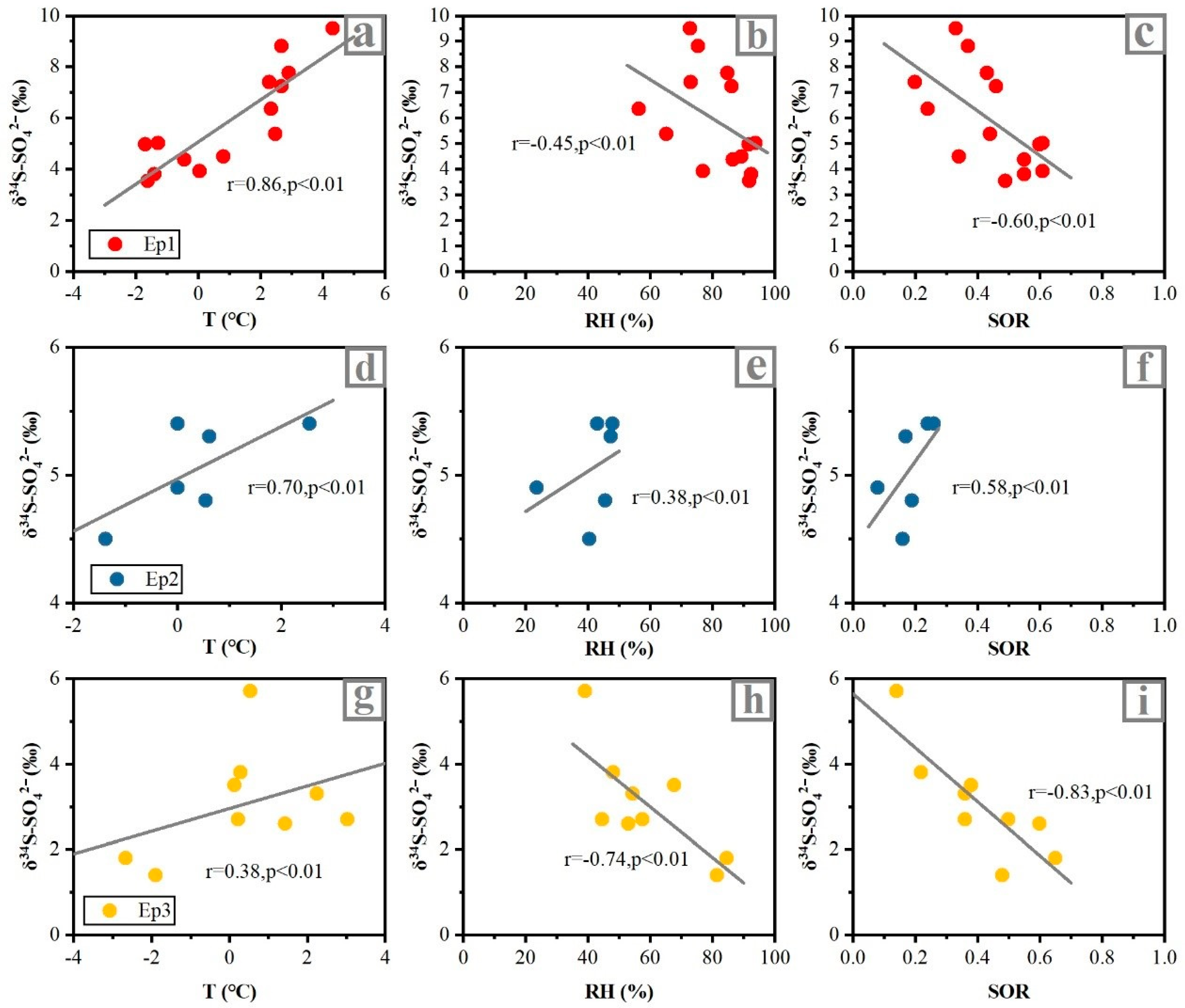
3.3.1. Sulfur Isotopic Compositions of Sulfate during the Haze Episodes

To better explore the reasons for the change of δ34Ssulfate values in polluted days after the implementation of CRP, three typical haze episodes during sampling were discussed in this study. The first haze episode (Ep1) started on 1 February 2017 and lasted until 1 August 2017, with average PM2.5 concentrations of 217.5 μg m−3 and the highest value is 339.7 μg m−3. The average δ34Ssulfate value is 5.9‰ during Ep1, which was 25.5% higher than that in the clean period. Furthermore, the measured δ34Ssulfate displayed significant positive correlations with temperature (T) (R = 0.86; p < 0.01). However, it was negatively correlated with relative humidity (RH) (R = −0.45; p < 0.01) and SO2 oxidation ratio (SOR = [SO42]/[SO42 + SO2]) (R = −0.60; p < 0.01) (Figure 4). The same negative correlation between the SOR and δ34Ssulfate value during the haze events observed in Nanjing, Beijing, and other places [21,29], indicating that the δ34Ssulfate values would be affected by different SO2 oxidation processes. In addition, the significant negative correlation between δ34Ssulfate and RH indicated that high RH promoted the isotope fractionation process in the water phase oxidation reaction of SO2 [29]. Combined with the backward trajectory analysis results (Figure 5), it was found that the air mass during Ep1 mainly came from cluster 2 and cluster 3, which might be affected by the sea salt sources with high δ34Ssulfate values (21‰) (Table S2) [30]. Therefore, before the implementation of CRP, the contribution of sea salt with high δ34Ssulfate might be one of the main reasons for the higher δ34Ssulfate in the pollution period than that in the clean period.
The haze episode 2 (Ep2) from 12 January 2018 to 14 January 2018, with average PM2.5 concentrations of 109.1 μg m−3 and the highest value was 155.5 μg m−3. Compared with Ep1, the mass concentration of PM2.5 in Ep2 decreased by 49.8%, which implies that the air quality of the Tianjin urban area has been significantly improved after the CRP. The average δ34Ssulfate value of Ep2 is 5.1‰, which was 15.7% lower than Ep1. Moreover, it was noteworthy that the δ34Ssulfate value of Ep2 was lower than that of the clean period during sampling, which was significantly different from the sampling period before the implementation of CRP (Figure 3b). In addition, the measured δ34Ssulfate of Ep2 was positively correlated with T (R = 0.70, p < 0.01). Since the BLH of Ep2 was significantly higher than that of Ep1 and Ep3 (Figure S1), the air mass had better diffusion ability, so the source and oxidation pathway of sulfate might change. Combined with the backward trajectory analysis (Figure 5), we found that the air mass during Ep2 mainly came from cluster 2 and cluster 4, which were mainly affected by the local sources and regional transportation in the southwest.
The haze episode 3 (Ep3) started on 10 January 2019 and lasted until 14 January 2019, with average PM2.5 concentrations of 127.9 μg m−3 and the highest value was 145.7 μg m−3. Compared with Ep2, the PM2.5 concentration of Ep3 did not decrease significantly but increased slightly, which implies that the environmental effect of the replacement of bulk coal was limited, and sulfate was still mainly derived from coal during the pollution period. Therefore, additional environmental protection policies (i.e., desulfurization and denitrification of coal) should be implemented to improve the atmospheric environment in the future. After the implementation of CRP, the air masses during Ep2 mainly came from cluster2 and cluster4, while the air masses during Ep3 mainly came from cluster1 and cluster3 (Figure 5). It was shown that the sources of air masses in the two episodes were similar, and they were mainly from local sources and regional transportation in the southwest (Figure 5). However, it was noteworthy that the δ34Ssulfate values in Ep3 decreased by 47.5% and 39.2% compared to Ep1 and Ep2, respectively. Since the regional transport of Ep2 and Ep3 is similar, it is speculated that the source has little influence on δ34Ssulfate, and the variations of this value may be mainly due to isotopic fractionation during the SO2 conversion to SO42− after the CRP.

3.3.2. Contributions of Oxidation Pathways to Sulfate Formation

Assuming the relative contribution of each source to sulfate aerosols was constant under the different air pollution conditions, the fractions of different sulfate formation pathways were calculated by the MIXSIAR model (Figure 6), and the contributions and uncertainties of different oxidation pathways were shown in Table S3. It could be found that the proportion of sulfate oxidation pathway in the three stages was different. As shown in Figure 6, the contribution of the TMI oxidation pathway and NO2 oxidation pathway in the three sampling stages was higher than that of the OH radical oxidation pathway and H2O2/O3 oxidation pathway, indicating that the formation pathway of sulfate in the Tianjin urban area was mainly dominated by a heterogeneous oxidation pathway. Except for Ep2, the contribution of TMI to sulfate during sampling was consistent with other cities in China [31,32], and the OH radical pathway was also consistent with values from the previous study (19–34%) in Beijing during the polluted season (Table S3) [32]. Thus, the source and formation pathways of sulfate have changed significantly during Ep2 when compared with the other two episodes.
Due to similar regional transport and local source contributions, we assumed that sulfate sources are similar in the winters of the 3 years. The NO2 oxidation pathway was the dominant sulfate oxidation pathway during Ep1 (Figure 6). Before the implementation of CRP, due to the NO2 pathway being more important in sulfate production under high NO2 and high RH conditions (Table 1) [33]. In addition, the high PM2.5 concentration during Ep1 (Table 1) might have amplified the formation of sulfate aerosol via the NO2 oxidation pathway through heterogeneous reaction, which was consistent with the research results in Beijing [17,27]. The TMIs oxidation pathway dominated the formation of sulfates during Ep2, and the contribution of Ep2 was about two times higher than that of Ep1. After the implementation of CRP, the increased contribution of the TMI pathway likely resulted from the higher efficiency of TMIs (e.g., Fe and Mn) in the atmosphere, which were emitted from local industrial sources in the haze events that enhanced the TMI oxidation rate [29].
Compared with Ep1, the contribution of sulfate formation by the OH oxidation pathway in Ep2 was significantly reduced after the CRP (Figure 6). This low contribution (5%) of gas-phase sulfate production was probably attributed to weak photochemistry in winter, high PM2.5 concentration, and extremely high heterogeneous and aqueous oxidations in haze episodes [21,34]. The present study highlighted that the oxidations of SO2 with NO2 and TMIs were the important formation pathways of sulfate aerosols in Tianjin, especially during the haze event.

4. Conclusions

After the implementation of CRP, the average concentration of PM2.5 in January 2018 and January 2019 dropped by approximately 60%. The trend of WSICs was consistent with PM2.5. The δ34Ssulfate in the clean period was lower than that in the pollution period before the CRP, which was mainly affected by sea salt sources with high δ34S. However, the δ34Ssulfate in the clean period was higher than that in the pollution period after the CRP, which was mainly due to the increase of heterogeneous oxidation contribution during the pollution period. The contribution of the TMI oxidation pathway and NO2 oxidation pathway in the three sampling stages is higher than that of the OH radical oxidation pathway and H2O2/O3 oxidation pathway, which shows that the formation pathway of sulfate in the Tianjin urban area is mainly dominated by heterogeneous oxidation pathway. Before the implementation of CRP, the NO2 oxidation pathway was the dominant sulfate oxidation pathway during Ep1, and the TMI oxidation pathway dominated the formation of sulfates after the implementation of CRP. Therefore, it should be noted that multiple energy-saving and emission reduction policies should be employed to further optimize the energy structure and therefore maximize the environmental benefits of energy conservation and emission reduction policies.

Supplementary Materials

The following supporting information can be downloaded at: https://www.mdpi.com/article/10.3390/ijerph191710966/s1, Figure S1: Time series of BLH during January 2017, 2018 and 2019; Figure S2: Consumption of electricity and industrial energy above scale, including coal, natural gas, crude oil, and others (coke, oil product, and thermal) in Tianjin from January 2016 to January 2019. Data from Tianjin Municipal People’s Government. Values for January and February each year are average consumption estimated by the sum of them. The SO2 and NO2 data during the sampling period come from the Air Quality Monitoring Station; Figure S3: Proportion of water-soluble ions in PM2.5 during sampling period; Table S1: Features of sampling phases; Table S2: The concentration of PM2.5, SO2, SO42− (μg/m3), and δ34Ssulfate values of air mass from different clusters; Table S3: The contribution and uncertainties of different oxidation pathway.

Author Contributions

Funding acquisition, X.-D.L.; Investigation, Y.C.; Methodology, S.D. and Q.L.; Visualization, S.D. and Y.C.; Writing—original draft, S.D. and Y.C.; Writing—review & editing, X.-D.L. All authors have read and agreed to the published version of the manuscript.

Funding

This work was supported by the National Natural Science Foundation of China (Grant No. 41773006).

Institutional Review Board Statement

Not applicable.

Informed Consent Statement

Not applicable.

Data Availability Statement

Data is contained within the article or Supplementary Material.

Conflicts of Interest

The authors declare no conflict of interest.

References

  1. Bai, W.; Zhao, X.; Yin, B.; Guo, L.; Zhang, W.; Wang, X.; Yang, W. Characteristics of PM2.5 in an industrial city of northern China: Mass concentrations, chemical composition, source apportionment, and health risk assessment. Int. J. Environ. Res. Public Health 2022, 19, 5443. [Google Scholar] [CrossRef] [PubMed]
  2. Ouyang, J.; Shao, Y.; Luo, M.; Zhang, J.L.; Dai, X.X.; Ma, L.L.; Xu, D.D. Exploration of the potential application of plutonium isotopes in source identification of sandstorm in the atmosphere of Beijing. Chin. Chem. Lett. 2022, 33, 3516–3521. [Google Scholar] [CrossRef]
  3. Wang, J.; Li, T.; Li, Z.; Fang, C. Study on the spatial and temporal distribution characteristics and influencing factors of particulate matter pollution in coal production cities in China. Int. J. Environ. Res. Public Health 2022, 19, 3228. [Google Scholar] [CrossRef]
  4. An, Z.; Huang, R.-J.; Zhang, R.; Tie, X.; Li, G.; Cao, J.; Zhou, W.; Shi, Z.; Han, Y.; Gu, Z.; et al. Severe haze in northern China: A synergy of anthropogenic emissions and atmospheric processes. Proc. Natl. Acad. Sci. USA 2019, 116, 8657–8666. [Google Scholar] [CrossRef]
  5. Zhang, Y.H.; Chen, Y.J.; Song, Y.Y.; Dong, C.; Cai, Z.W. Atmospheric pressure gas chromatography-tandem mass spectrometry analysis of fourteen emerging polycyclic aromatic sulfur heterocycles in PM2.5. Chin. Chem. Lett. 2021, 32, 801–804. [Google Scholar] [CrossRef]
  6. Tao, J.; Zhang, L.; Cao, J.; Zhang, R. A review of current knowledge concerning PM2.5 chemical composition, aerosol optical properties and their relationships across China. Atmos. Chem. Phys. 2017, 17, 9485–9518. [Google Scholar]
  7. Feng, X.Q.; Li, Q.K.; Tao, Y.L.; Ding, S.Y.; Chen, Y.Y.; Li, X.D. Impact of Coal Replacing Project on atmospheric fine aerosol nitrate loading and formation pathways in urban Tianjin: Insights from chemical composition and 15N and 18O isotope ratios. Sci. Total Environ. 2020, 708, 134797. [Google Scholar] [PubMed]
  8. Wu, G.; Tian, W.; Zhang, L.; Yang, H. The Chinese spring festival impact on air quality in China: A critical review. Int. J. Environ. Res. Public Health 2022, 19, 9074. [Google Scholar] [CrossRef] [PubMed]
  9. Chen, C.; Sun, Y.L.; Xu, W.Q.; Du, W.; Zhou, L.B.; Han, T.T.; Wang, Q.Q.; Fu, P.Q.; Wang, Z.F.; Gao, Z.Q. Characteristics and sources of submicron aerosols above the urban canopy (260 m) in Beijing, China during 2014 APEC summit. Atmos. Chem. Phys. 2015, 15, 12879–12895. [Google Scholar] [CrossRef]
  10. Su, W.J.; Liu, C.; Hu, Q.H.; Fan, G.Q.; Xie, Z.Q.; Huang, X.; Zhang, T.S.; Chen, Z.Y.; Dong, Y.S.; Ji, X.G. Characterization of ozone in the lower troposphere during the 2016 G20 conference in Hangzhou. Sci. Rep. 2017, 7, 17368. [Google Scholar] [CrossRef]
  11. Chen, H.; Chen, W.Y. Potential impact of shifting coal to gas and electricity for building sectors in 28 major northern cities of China. Appl. Energy 2019, 236, 1049–1061. [Google Scholar] [CrossRef]
  12. Lin, B.; Jia, Z. Economic, energy and environmental impact of coal-to-electricity policy in China: A dynamic recursive CGE study. Sci. Total Environ. 2020, 698, 134241. [Google Scholar] [CrossRef] [PubMed]
  13. Zhang, C.Q.; Yang, J.J. Economic benefits assessments of “coal-to-electricity” project in rural residents heating based on life cycle cost. J. Clean. Prod. 2019, 213, 217–224. [Google Scholar] [CrossRef]
  14. Ren, Y.Q.; Wang, G.H.; Wu, C.; Wang, J.Y.; Li, J.J.; Zhang, L.; Han, Y.N.; Liu, L.; Cao, C.; Cao, J.J.; et al. Changes in concentration, composition and source contribution of atmospheric organic aerosols by shifting coal to natural gas in Urumqi. Atmos. Environ. 2017, 148, 306–315. [Google Scholar] [CrossRef]
  15. Pang, J.; Jian, W.U.; Zhong, M.A.; Liang, L.N.; Zhang, T.T. Air pollution abatement effects of replacing coal with natural gas for central heating in cities of China. China Environ. Sci. 2015, 35, 55–61. [Google Scholar]
  16. Zhang, J.P.; Ning, Y.C.; Liu, C.L.; Zheng, L.I.; Wang, H.H.; Chen, L. Monitoring and analysis of effect of project “Replacing Coal With Electricity” improving atmospheric environmental quality in mentougou district, Beijing. J. Ecol. Rural Environ. 2017, 33, 898–906. [Google Scholar]
  17. Wang, G.; Zhang, R.; Gomez, M.E.; Yang, L.; Zamora, M.L.; Hu, M.; Lin, Y.; Peng, J.; Guo, S.; Meng, J. Persistent sulfate formation from London Fog to Chinese haze. Proc. Natl. Acad. Sci. USA 2016, 113, 13630–13635. [Google Scholar] [CrossRef]
  18. Huang, R.J.; Zhang, Y.L.; Bozzetti, C.; Ho, K.F.; Cao, J.J.; Han, Y.M.; Daellenbach, K.R.; Slowik, J.G.; Platt, S.M.; Canonaco, F. High secondary aerosol contribution to particulate pollution during haze events in China. Nature 2014, 514, 218–222. [Google Scholar] [CrossRef]
  19. Chen, S.; Guo, Z.; Guo, Z.; Guo, Q.; Zhang, Y.; Zhu, B.; Zhang, H. Sulfur isotopic fractionation and its implication: Sulfate formation in PM2.5 and coal combustion under different conditions. Atmos. Res. 2017, 194, 142–149. [Google Scholar] [CrossRef]
  20. Leung, F.Y.; Colussi, A.J.; Hoffmann, M.R. Sulfur isotopic fractionation in the gas-phase oxidation of sulfur dioxide initiated by hydroxyl radicals. J. Phys. Chem. A 2001, 105, 8073–8076. [Google Scholar] [CrossRef]
  21. Li, J.H.Y.; Zhang, Y.L.; Cao, F.; Zhang, W.Q.; Fan, M.Y.; Lee, X.H.; Michalski, G. Stable sulfur isotopes revealed a major role of transition-metal-ion catalyzed SO2 oxidation in haze episodes. Environ. Sci. Technol. 2020, 54, 2626–2634. [Google Scholar] [CrossRef] [PubMed]
  22. Wei, L.F.; Yue, S.Y.; Zhao, W.Y.; Yang, W.Y.; Zhang, Y.J.; Ren, L.J.; Han, X.K.; Guo, Q.J.; Sun, Y.L.; Wang, Z.F. Stable sulfur isotope ratios and chemical compositions of fine aerosols (PM2.5) in Beijing, China. Sci. Total Environ. 2018, 633, 1156–1164. [Google Scholar] [CrossRef] [PubMed]
  23. Ding, T.; Valkiers, S.; Kipphardt, H.; De Bievre, P.; Taylor, P.; Gonfiantini, R.; Krouse, R. Calibrated sulfur isotope abundance ratios of three IAEA sulfur isotope reference materials and V-CDT with a reassessment of the atomic weight of sulfur. Geochim. Cosmochim. Acta 2001, 65, 2433–2437. [Google Scholar] [CrossRef]
  24. Guo, Z.; Shi, L.; Chen, S.; Jiang, W.; Wei, Y.; Rui, M.; Zeng, G. Sulfur isotopic fractionation and source appointment of PM2.5 in Nanjing region around the second session of the Youth Olympic Games. Atmos. Res. 2016, 174, 9–17. [Google Scholar] [CrossRef]
  25. Sakata, M.; Ishikawa, T.; Mitsunobu, S. Effectiveness of sulfur and boron isotopes in aerosols as tracers of emissions from coal burning in Asian continent. Atmos. Environ. 2013, 67, 296–303. [Google Scholar] [CrossRef]
  26. Sinha, B.; Hoppe, P.; Huth, J.; Foley, S.; Andreae, M. Sulfur isotope analyses of individual aerosol particles in the urban aerosol at a central European site (Mainz, Germany). Atmos. Chem. Phys. 2008, 8, 7217–7238. [Google Scholar] [CrossRef]
  27. Cheng, Y.; Zheng, G.; Wei, C.; Mu, Q.; Zheng, B.; Wang, Z.; Gao, M.; Zhang, Q.; He, K.; Carmichael, G. Reactive nitrogen chemistry in aerosol water as a source of sulfate during haze events in China. Sci. Adv. 2016, 2, e1601530. [Google Scholar] [CrossRef]
  28. Harris, E.; Sinha, B.; Hoppe, P.; Crowley, J.; Ono, S.; Foley, S. Sulfur isotope fractionation during oxidation of sulfur dioxide: Gas-phase oxidation by OH radicals and aqueous oxidation by H2O2, O3 and iron catalysis. Atmos. Chem. Phys. 2012, 12, 407–423. [Google Scholar] [CrossRef]
  29. Fan, M.Y.; Zhang, Y.L.; Lin, Y.C.; Li, J.; Fu, P. Roles of sulfur oxidation pathways in the variability in stable sulfur isotopic composition of sulfate aerosols at an urban site in Beijing, China. Environ. Sci. Technol. Lett. 2020, 7, 883–888. [Google Scholar] [CrossRef]
  30. Tostevin, R.; Turchyn, A.V.; Farquhar, J.; Johnston, D.T.; Eldridge, D.L.; Bishop, J.K.; McIlvin, M. Multiple sulfur isotope constraints on the modern sulfur cycle. Earth Planet. Sci. Lett. 2014, 396, 14–21. [Google Scholar] [CrossRef]
  31. Alexander, B.; Park, R.J.; Jacob, D.J.; Gong, S. Transition metal-catalyzed oxidation of atmospheric sulfur: Global implications for the sulfur budget. J. Geophys. Res. Atmos. 2009, 114, D02309. [Google Scholar] [CrossRef]
  32. Shao, J.; Chen, Q.; Wang, Y.; Lu, X.; Alexander, B. Heterogeneous sulfate aerosol formation mechanisms during wintertime Chinese haze events: Air quality model assessment using observations of sulfate oxygen isotopes in Beijing. Atmos. Chem. Phys. 2019, 19, 6107–6123. [Google Scholar] [CrossRef]
  33. Xue, J.; Yu, X.; Yuan, Z.; Griffith, S.M.; Lau, A.; Seinfeld, J.H.; Yu, J.Z. Efficient control of atmospheric sulfate production based on three formation regimes. Nat. Geosci. 2019, 12, 977–982. [Google Scholar] [CrossRef]
  34. Han, S.Q.; Wu, J.H.; Zhang, Y.F.; Cai, Z.Y.; Feng, Y.C.; Yao, Q.; Li, X.J.; Liu, Y.W.; Zhang, M. Characteristics and formation mechanism of a winter haze–fog episode in Tianjin, China. Atmos. Environ. 2014, 98, 323–330. [Google Scholar] [CrossRef]
Figure 1. Sampling site located in the Tianjin.
Ijerph 19 10966 g001
Figure 2. Time series of pollutant concentrations (PM2.5, SNA, SO2, NO2 and O3), SOR, NOR, δ34S of sulfates and the meteorological data (RH and T) during six campaigns. The gray shaded area indicated a polluted period (PM2.5 ≥ 75 μg m−3).
Ijerph 19 10966 g002
Figure 3. (a) Average δ34S-SO42−during four sampling periods, (b) Box plots of δ34S-SO42− during the clean period (blue boxes) and polluted period (grey boxes).
Ijerph 19 10966 g003
Figure 4. Relationships between δ34S-SO42− and temperature (T), relative humidity (RH), and SOR in Tianjin during Ep1 (ac), Ep2 (df), Ep3 (gi).
Ijerph 19 10966 g004
Figure 5. 48-h backward trajectory of (a): January2017, (b): January2018, (c): January2019.
Ijerph 19 10966 g005
Figure 6. (a) Rayleigh distillation model of sulfate production. Black circles are the measured δ34Ssulfate values from this study. The green line indicates the δ34Ssulfate when SO2 is oxidized solely by H2O2 and O3. The red line indicates the δ34Ssulfate when SO2 is oxidized solely by OH. The blue line indicates the δ34Ssulfate when SO2 is oxidized solely by NO2. The purple line indicates the δ34Ssulfate when SO2 is oxidized solely by TMI oxidation. The black line is the best fit of observed δ34Ssulfate, showing an average εobs value of +6.6 ± 2.1‰. (b) Contribution of each formation pathway based on the Bayesian model calculation.
Ijerph 19 10966 g006
Table 1. PM2.5 (μg m−3), water-soluble ions concentrations (μg m−3), Meteorological parameters: relative humidity (RH, %), temperature (T, °C), wind speed (WS, m s−1), gaseous contaminants concentrations (μg m−3): SO2, NO2, O3, sulfur oxidation ratio (SOR) and nitrogen oxidation ratio (NOR) of the sampling campaigns (C: clean period; Ep: haze episode).
January 2017January 2018January 2019
All
(n = 28)
C
(n = 6)
Ep1
(n = 14)
All
(n = 30)
C
(n = 19)
Ep2
(n = 6)
All
(n = 40)
C
(n = 27)
Ep3
(n = 9)
PM2.5151.6 ± 86.259.7 ± 19.2217.5 ± 72.560.7 ± 39.235.5 ± 17.8109.1 ± 26.565.4 ± 43.339.0 ± 18.2127.9 ± 16.7
Na+0.7 ± 0.50.3 ± 0.11.1 ± 0.30.3 ± 0.20.2 ± 0.10.4 ± 0.10.3 ± 0.10.2 ± 0.10.4 ± 0.1
NH4+15.1 ± 13.23.1 ± 1.625.3 ± 11.39.2 ± 7.84.1 ± 3.418.1 ± 4.87.6 ± 6.13.9 ± 2.515.8 ± 3.1
K+1.0 ± 0.80.3 ± 0.11.7 ± 0.70.9 ± 0.60.5 ± 0.31.6 ± 0.30.9 ± 0.60.6 ± 0.41.4 ± 0.3
Ca2+0.3 ± 0.30.4 ± 0.20.4 ± 0.40.3 ± 0.20.2 ± 0.20.3 ± 00.1 ± 0.10.1 ± 0.10.2 ± 0.1
Mg2+0.04 ± 0.030.04 ± 0.040.04 ± 0.020.01 ± 0.020.01 ± 0.020.02 ± 0.000.03 ± 0.010.02 ± 0.100.03 ± 0.01
Cl5.2 ± 5.01.5 ± 0.78.4 ± 5.24.2 ± 4.32.0 ± 1.86.0 ± 1.44.0 ± 2.63.1 ± 2.35.0 ± 1.4
NO322.3 ± 19.44.54 ± 2.6537.3 ± 16.910.0 ± 9.83.82 ± 3.0724.0 ± 8.911.5 ± 9.55.65 ± 3.8324.1 ± 4.6
SO42−24.6 ± 21.25.3 ± 3.240.8 ± 18.75.0 ± 3.23.0 ± 1.78.4 ± 2.45.6 ± 5.72.2 ± 1.114.7 ± 3.7
RH60.6 ± 24.228.5 ± 7.481.1 ± 11.434.8 ± 14.431.2 ± 16.141.3 ± 9.129.4 ± 18.319.4 ± 3.658.9 ± 15.9
T0.9 ± 1.90.5 ± 1.31.0 ± 2.0−0.7 ± 2.31.4 ± 2.50.4 ± 1.30.6 ± 2.40.5 ± 2.70.4 ± 1.8
WS1.4 ± 0.72.3 ± 0.81.0 ± 0.41.5 ± 0.41.6 ± 0.51.4 ± 0.31.5 ± 0.71.7 ± 0.81.1 ± 0.3
SO228.1 ± 11.313.8 ± 3.831.1 ± 6.717.0 ± 10.111.0 ± 6.126.2 ± 6.318.7 ± 13.116.2 ± 11.316.2 ± 8.5
NO278.9 ± 33.836.5 ± 8.6101.0 ± 25.257.8 ± 26.145.1 ± 23.174.7 ± 13.563.6 ± 24.952.9 ± 22.682.5 ± 11.8
O336.1 ± 19.558.8 ± 11.121.9 ± 12.927.7 ± 17.833.3 ± 18.822.0 ± 10.322.9 ± 16.826.4 ± 17.414.8 ± 12.9
SOR0.3 ± 0.20.2 ± 0.10.4 ± 0.10.2 ± 0.10.2 ± 0.10.2 ± 0.10.2 ± 0.20.1 ± 0.10.4 ± 0.2
NOR0.1 ± 0.10.1 ± 0.10.2 ± 0.10.1 ± 0.10.05 ± 0.10.2 ± 0.10.1 ± 0.10.1 ± 0.10.2 ± 0.01
Publisher’s Note: MDPI stays neutral with regard to jurisdictional claims in published maps and institutional affiliations.

