
Spatial-Temporal Changes and Associated Determinants of Global Heating Degree Days


Abstract
:1. Introduction
2. Materials and Methods
2.1. Materials
2.2. Methods
2.2.1. Spatial-Temporal Changes in Global Heating Degree Days
2.2.2. Associated Determinants of Global Heating Degree Days and Their Interannual Change Rates
3. Results and Discussion
3.1. Spatial-Temporal Changes in Global Heating Degree Days
3.1.1. Spatial Variations of Global Heating Degree Days
3.1.2. Interannual Spatial-Temporal Changes in Global Heating Degree Days
3.2. Associated Determinants of Global Heating Degree Days
3.2.1. Associated Determinants of Spatial Variation of Global Heating Degree Days
3.2.2. Associated Determinants of the Interannual Change Rates of Global Heating Degree Days
3.2.3. Limitations and Future Work
4. Conclusions
- (1)
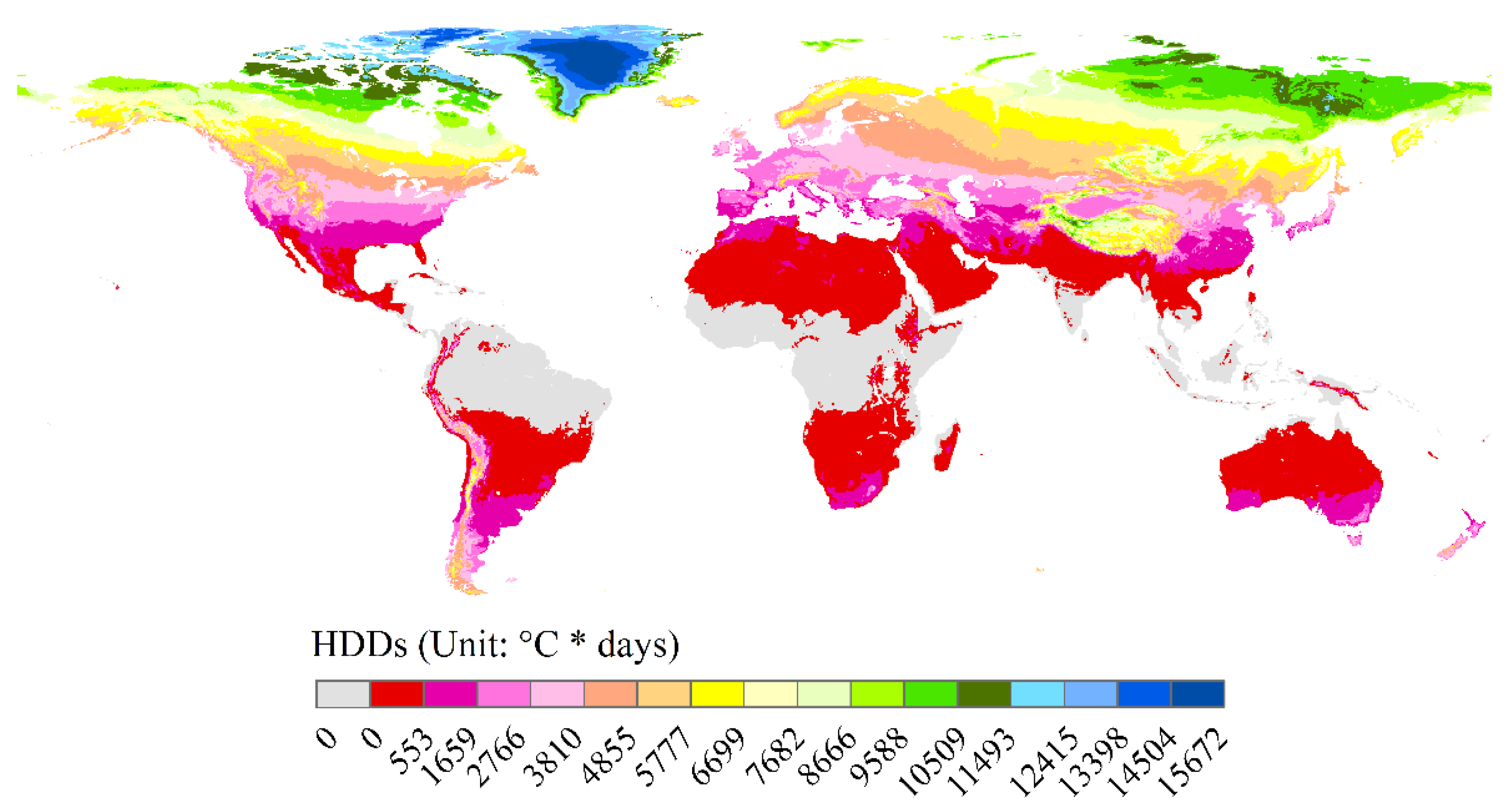
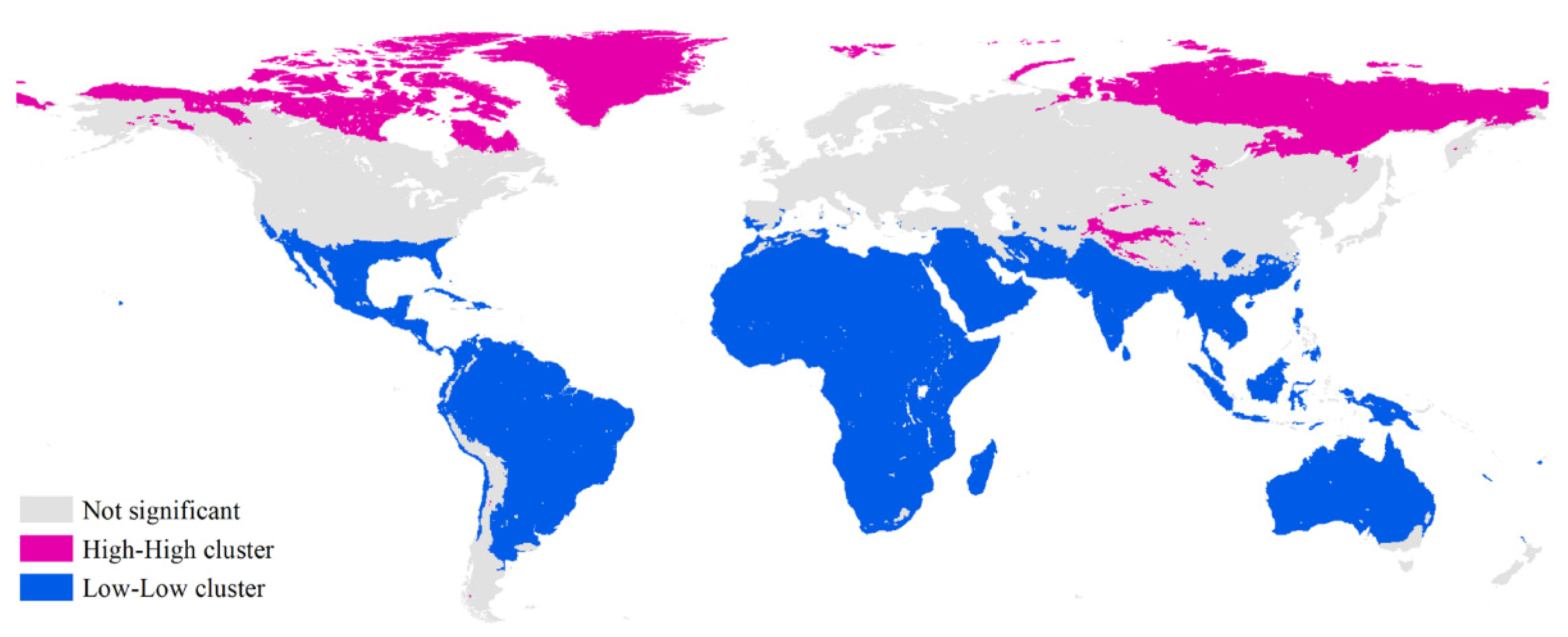
- The global HDDs showed extremely obvious spatial distribution laws, which generally became larger in places with higher latitudes and altitudes. The largest HDD was 15,672 °C * days, which occurred in central Greenland. High spatial positive correlations existed for global HDDs, and both HH and LL clusters existed.
- (2)
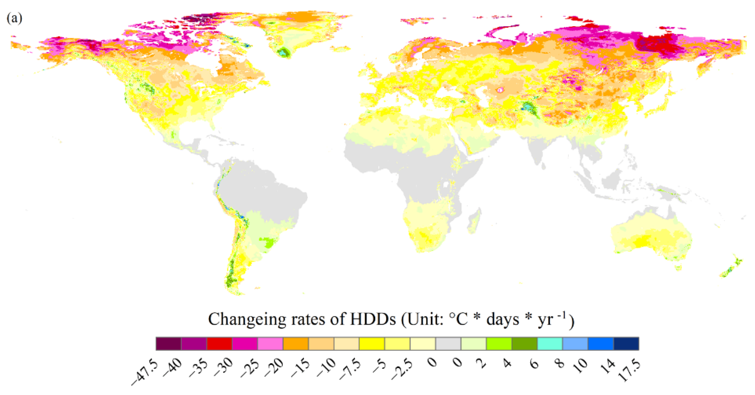
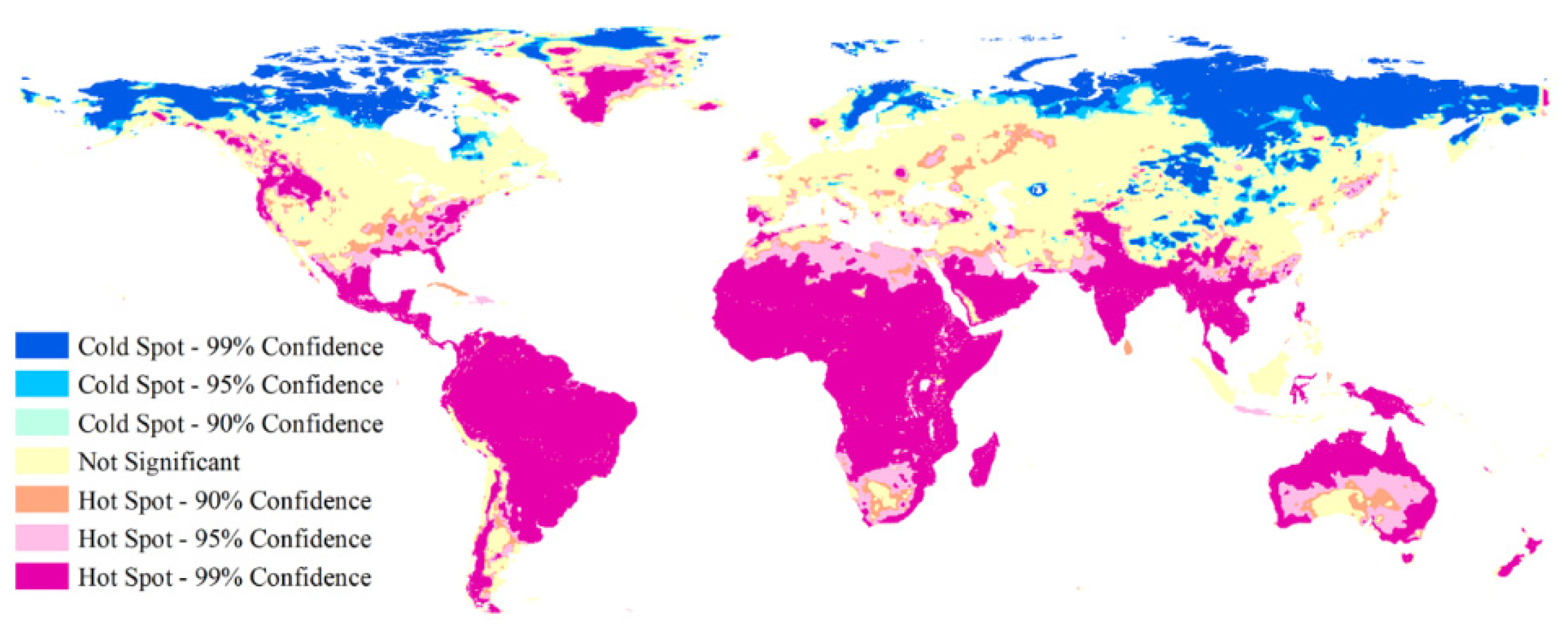
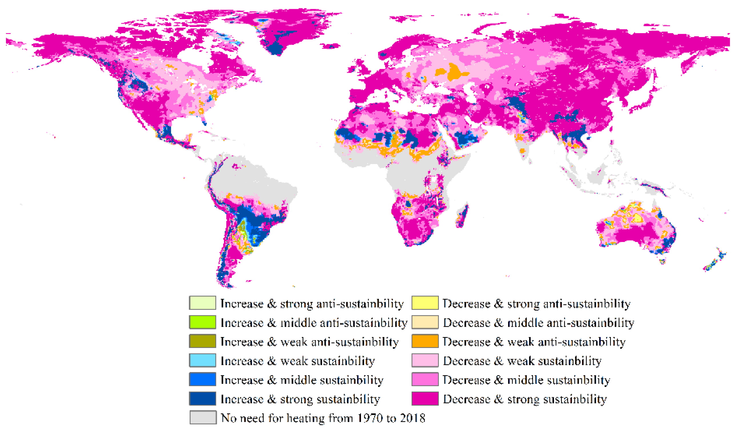
- Most global change rates of HDDs were negative during the past 49 years (over the period 1970–2018), and they generally decreased to a greater extent in areas with higher latitudes. The negative rates mainly occurred in southeastern South America, the Andes, Mexico, the northwestern United States, southern Greenland, southern North Africa, the southern Arabian peninsula, eastern Turkey, northern South Asia, and its northern surrounding regions, northern Southeast Asia and southwestern China, southeastern Australia, and New Zealand. Most of the abovementioned change rates passed the significant level of 0.1. High spatial positive correlations existed for the variation rates of global HDDs, and both cold and hot spots existed. The vast majority of the global HDDs showed sustainability trends in the future.
- (3)
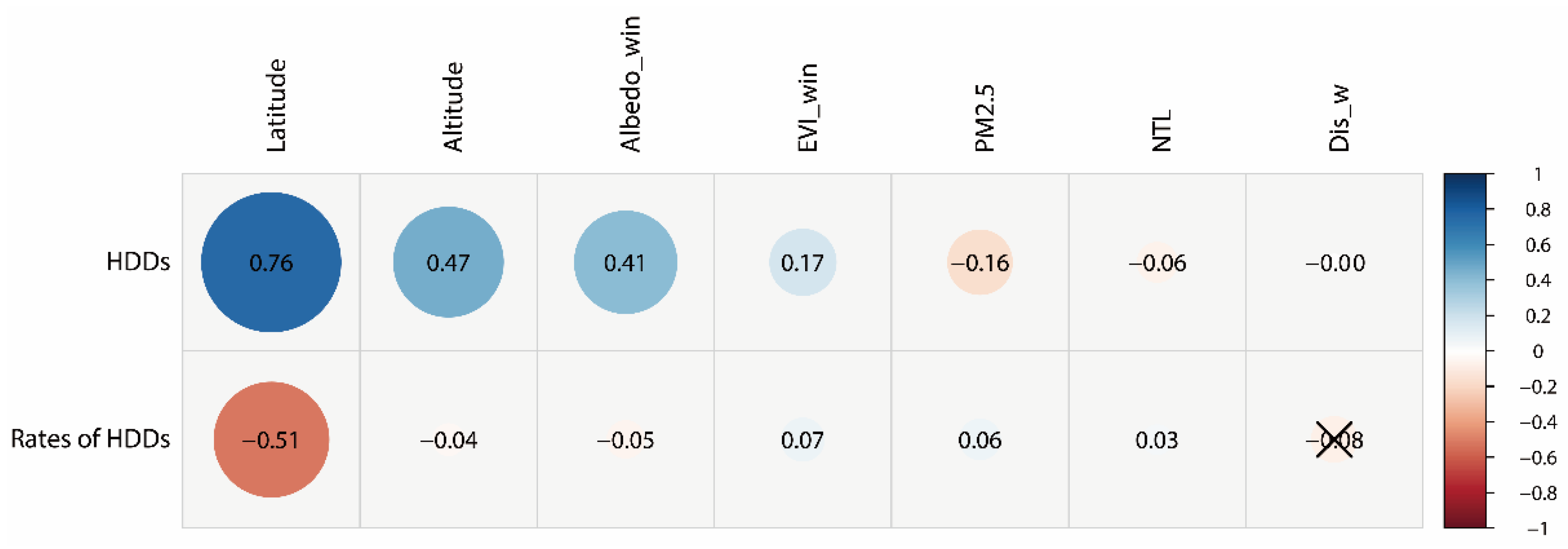
- The HDDs were significantly positively partially correlated with latitude, altitude, mean albedo, and EVI during winter, and significantly negatively partially correlated with annual mean PM2.5 concentration, NTL intensity, and distance to large waterbodies (seas or oceans) (p = 0.000). The interannual change rates of HDDs were significantly negatively partially correlated with latitude, altitude, mean albedo during winter, and distance to large waterbodies, and significantly positively partially correlated with the mean EVI during winter, annual PM2.5 concentration and NTL intensity (p = 0.000).
- (4)
- Both the predicted HDDs and their interannual change rates by GRNN algorithm were significantly highly correlated with their actual values (p = 0.000). The RMSEs of HDDs and their variation rates for the testing samples were 564.08 °C * days and 3.59 °C * days * year−1, respectively.
- (5)
- Our findings could support the scientific response to climate warming, the construction of living environments, sustainable development, etc. In the future, the global HDDs should be derived from other data, especially the observed data for the related studies. Moreover, more influence factors should be considered, such as the greenhouse gas concentration, atmospheric circulation indices, landscape composition and pattern, remotely sensed indices, the sky view factor, heat release, population density, etc. More accurate and detailed mechanisms should be explored under different contexts at multiple scales during different periods. More effective methods should be adopted, such as experimental observation, numerical simulation, etc.
Author Contributions
Funding
Institutional Review Board Statement
Informed Consent Statement
Data Availability Statement
Conflicts of Interest
References
- Intergovernmental Panel on Climate Change (IPCC). Climate Change 2013: The Physical Science Basis; IPCC: New York, NY, USA, 2014. [Google Scholar]
- Valipour, M.; Bateni, S.M.; Jun, C. Global surface temperature: A new insight. Climate 2021, 9, 81. [Google Scholar] [CrossRef]
- Orimoloye, I.R.; Mazinyo, S.P.; Kalumba, A.M.; Ekundayo, O.Y.; Nel, W. Implications of climate variability and change on urban and human health: A review. Cities 2019, 91, 213–223. [Google Scholar] [CrossRef]
- Kownacki, K.L.; Gao, C.; Kuklane, K.; Wierzbicka, A. Heat stress in indoor environments of scandinavian urban areas: A literature review. Int. J. Environ. Res. Public Health 2019, 16, 560. [Google Scholar] [CrossRef] [PubMed] [Green Version]
- Costa, A.; Keane, M.M.; Torrens, J.I.; Corry, E. Building operation and energy performance: Monitoring, analysis and optimisation toolkit. Appl. Energy 2013, 101, 310–316. [Google Scholar] [CrossRef]
- Waite, M.; Cohen, E.; Torbey, H.; Piccirilli, M.; Tian, Y.; Modi, V. Global trends in urban electricity demands for cooling and heating. Energy 2017, 127, 786–802. [Google Scholar] [CrossRef] [Green Version]
- Rosen, M.A. Energy sustainability with a focus on environmental perspectives. Earth Syst. Environ. 2021, 1–14. [Google Scholar] [CrossRef]
- Biardeau, L.T.; Davis, L.W.; Gertler, P.; Wolfram, C. Heat exposure and global air conditioning. Nat. Sustain. 2020, 3, 25–28. [Google Scholar] [CrossRef]
- Li, X.X. Linking residential electricity consumption and outdoor climate in a tropical city. Energy 2018, 157, 734–743. [Google Scholar] [CrossRef]
- Isaac, M.; Vuuren, D.P.V. Modeling global residential sector energy demand for heating and air conditioning in the context of climate change. Energy Policy 2009, 37, 507–521. [Google Scholar] [CrossRef]
- London Climate Change Partnership (LCCP). London’s Commercial Building Stock and Climate Change Adaptation: Design, Finance and Legal Implications; London Climate Change Partnership: London, UK, 2009. [Google Scholar]
- Mistry, M.N. Historical global gridded degree-days: A high-spatial resolution database of CDD and HDD. Geosci. Data J. 2019, 6, 214–221. [Google Scholar] [CrossRef] [Green Version]
- Islam, A.M.T.; Ahmed, I.; Rahman, M.S. Trends in cooling and heating degree-days overtimes in Bangladesh? An investigation of the possible causes of changes. Nat. Hazards 2020, 101, 879–909. [Google Scholar] [CrossRef]
- Atalla, T.; Gualdi, S.; Lanza, A. A global degree days database for energy-related applications. Energy 2018, 143, 1048–1055. [Google Scholar] [CrossRef] [Green Version]
- Petri, Y.; Caldeira, K. Impacts of global warming on residential heating and cooling degree-days in the United States. Sci. Rep. 2015, 5, 12427. [Google Scholar] [CrossRef] [Green Version]
- Giannakopoulos, C.; Psiloglou, B.; Lemesios, G.; Xevgenos, D.; Papadaskalopoulou, C.; Karali, A.; Varotsos, K.V.; Zachariou-Dodou, M.; Moustakas, K.; Ioannou, K. Climate change impacts, vulnerability and adaptive capacity of the electrical energy sector in Cyprus. Reg. Environ. Chang. 2016, 16, 1891–1904. [Google Scholar] [CrossRef]
- Ren, Y.; Ren, G.; Qian, H. Change scenarios of China’s provincial climate-sensitive components of energy consumption. Geogr. Res. 2009, 28, 36–44. [Google Scholar]
- Morakinyo, T.E.; Ren, C.; Shi, Y.; Lau, K.K.L.; Tong, H.W.; Choy, C.W.; Ng, E. Estimates of the impact of extreme heat events on cooling energy demand in Hong Kong. Renew. Energy 2019, 142, 73–84. [Google Scholar] [CrossRef]
- Zhang, H.; Zhang, X.; Sun, Z.; Tang, G. A study on degree-day’s change in China in the past fifty years. Trans. Atmos. Sci. 2010, 33, 593–599. [Google Scholar]
- Spinoni, J.; Vogt, J.V.; Barbosa, P.; Dosio, A.; McCormick, N.; Bigano, A.; Füssel, H.M. Changes of heating and cooling degree-days in Europe from 1981 to 2100. Int. J. Climatol. 2018, 38, e191–e208. [Google Scholar] [CrossRef]
- Schatz, J.; Kucharik, C.J. Urban heat island effects on growing seasons and heating and cooling degree days in Madison, Wisconsin USA. Int. J. Climatol. 2016, 36, 4873–4884. [Google Scholar] [CrossRef] [Green Version]
- Massetti, L.; Petralli, M.; Brandani, G.; Orlandini, S. An approach to evaluate the intra-urban thermal variability in summer using an urban indicator. Environ. Pollut. 2014, 192, 259–265. [Google Scholar] [CrossRef]
- Limones-Rodríguez, N.; Marzo-Artigas, J.; Pita-López, M.F.; Díaz-Cuevas, M.P. The impact of climate change on air conditioning requirements in Andalusia at a detailed scale. Theor. Appl. Climatol. 2018, 134, 1047–1063. [Google Scholar] [CrossRef]
- Jiang, F.; Li, X.; Wei, B.; Hu, R.; Li, Z. Observed trends of heating and cooling degree-days in Xinjiang Province, China. Theor. Appl. Climatol. 2009, 97, 349–360. [Google Scholar] [CrossRef]
- Rodell, M.; Houser, P.R.; Jambor, U.; Gottschalck, J.; Mitchell, K.; Meng, C.J.; Arsenault, K.; Cosgrove, B.; Radakovich, J.; Bosilovich, M. Land data assimilation systems. Bull. Am. Meteorol. Soc. 2004, 85, 381–394. [Google Scholar] [CrossRef] [Green Version]
- Ji, L.; Senay, G.B.; Verdin, J.P. Evaluation of the global land data assimilation system (GLDAS) air temperature data products. J. Hydrometeorol. 2015, 16, 2463–2480. [Google Scholar] [CrossRef]
- Huang, X.; Huang, J.; Wen, D.; Li, J. An updated MODIS global urban extent product (MGUP) from 2001 to 2018 based on an automated mapping approach. Int. J. Appl. Earth Obs. Geoinf. 2021, 95, 102255. [Google Scholar] [CrossRef]
- Hammer, M.S.; Donkelaar, A.V.; Li, C.; Lyapustin, A.; Martin, R.V. Global estimates and long-term trends of fine particulate matter concentrations (1998–2018). Environ. Sci. Technol. 2020, 54, 7879–7890. [Google Scholar] [CrossRef]
- Shen, X.; Liu, B. Changes in the timing, length and heating degree days of the heating season in central heating zone of China. Sci. Rep. 2016, 6, 33384. [Google Scholar] [CrossRef]
- Shen, X.; Liu, B.; Zhou, D. Spatiotemporal changes in the length and heating degree days of the heating period in Northeast China. Meteorol. Appl. 2017, 24, 135–141. [Google Scholar] [CrossRef] [Green Version]
- Li, Y.; Wang, L.; Zhou, H.; Zhao, G.; Ling, F.; Li, X.; Qiu, J. Urbanization effects on changes in the observed air temperatures during 1977–2014 in China. Int. J. Climatol. 2019, 39, 251–265. [Google Scholar] [CrossRef] [Green Version]
- Sun, Z.; Zhan, D.; Jin, F. Spatio-temporal characteristics and geographical determinants of air quality in cities at the prefecture level and above in China. Chin. Geogr. Sci. 2019, 29, 138–146. [Google Scholar] [CrossRef]
- Pal, S.; Dutta, S.; Nasrin, T.; Chattopadhyay, S. Hurst exponent approach through rescaled range analysis to study the time series of summer monsoon rainfall over northeast India. Theor. Appl. Climatol. 2020, 142, 581–587. [Google Scholar] [CrossRef]
- Jovanovic, D.; Jovanovic, T.; Mejia, A.; Hathaway, J.; Daly, E. Technical note: Long-term persistence loss of urban streams as a metric for catchment classification. Hydrol. Earth Syst. Sci. 2018, 22, 3551–3559. [Google Scholar] [CrossRef] [Green Version]
- Zhang, W.; Wang, L.C.; Xiang, F.F.; Qin, W.M.; Jiang, W.X. Vegetation dynamics and the relations with climate change at multiple time scales in the Yangtze River and Yellow River Basin, China. Ecol. Indic. 2015, 110, 117–126. [Google Scholar] [CrossRef]
- Yan, E.P.; Lin, H.; Dang, Y.F.; Xia, C.Z. The spatiotemporal changes of vegetation cover in Beijing-Tianjin sandstorm source control region during 2000–2012. Acta Ecol. Sin. 2014, 34, 5007–5020. [Google Scholar]
- Specht, D.F. A general regression neural network. IEEE Trans. Neural Netw. 1991, 2, 568–576. [Google Scholar] [CrossRef] [Green Version]
- Rooki, R. Application of general regression neural network (GRNN) for indirect measuring pressure loss of Herschel–Bulkley drilling fluids in oil drilling. Measurement 2016, 85, 184–191. [Google Scholar] [CrossRef]
- Heddam, S. Generalized regression neural network (GRNN)-based approach for colored dissolved organic matter (CDOM) retrieval: Case study of Connecticut River at Middle Haddam Station, USA. Environ. Monit. Assess. 2014, 186, 7837–7848. [Google Scholar] [CrossRef] [PubMed]
- Santamouris, M.; Fiorito, F. On the impact of modified urban albedo on ambient temperature and heat related mortality. Solar Energy 2021, 216, 493–507. [Google Scholar] [CrossRef]
- Kim, J.E.; Lague, M.M.; Pennypacker, S.; Dawson, E.; Swann, A.L.S. Evaporative resistance is of equal importance as surface albedo in high-latitude surface temperatures due to cloud feedbacks. Geophys. Res. Lett. 2020, 47, e2019GL085663. [Google Scholar] [CrossRef]
- Li, Y.; Wang, L.; Liu, M.; Zhao, G.; Mao, Q. Associated determinants of surface urban heat islands across 1449 cities in China. Adv. Meteorol. 2019, 2019, 4892714. [Google Scholar] [CrossRef] [Green Version]
- Chudnovsky, A.; Ben-Dor, E.; Saaroni, H. Diurnal thermal behavior of selected urban objects using remote sensing measurements. Energy Build. 2004, 36, 1063–1074. [Google Scholar] [CrossRef]
- Li, Y.; Zhao, M.; Motesharrei, S.; Mu, Q.; Kalnay, E.; Li, S. Local cooling and warming effects of forests based on satellite observations. Nat. Commun. 2015, 6, 6603. [Google Scholar] [CrossRef] [PubMed] [Green Version]
- Cao, C.; Lee, X.; Liu, S.; Schultz, N.; Xiao, W.; Zhang, M.; Zhao, L. Urban heat islands in China enhanced by haze pollution. Nat. Commun. 2016, 7, 12509. [Google Scholar] [CrossRef] [PubMed]
- Han, W.; Li, Z.; Wu, F.; Zhang, Y.; Guo, J.; Su, T.; Cribb, M.; Fan, J.; Chen, T.; Wei, J.; et al. The mechanisms and seasonal differences of the impact of aerosols on daytime surface urban heat island effect. Atmos. Chem. Phys. 2020, 20, 6479–6493. [Google Scholar] [CrossRef]
- Vose, R.S.; Karl, T.R.; Easterling, D.R.; Williams, C.N.; Menne, M.J. Climate (communication arising): Impact of land-use change on climate. Nature 2004, 427, 213–214. [Google Scholar] [CrossRef]
- Wang, J.; Yan, Z.W. Urbanization-related warming in local temperature records: A review. Atmos. Ocean. Sci. Lett. 2016, 9, 129–138. [Google Scholar] [CrossRef] [Green Version]
- Chen, F. Response Characteristics of Air Temperature Changes at Different Altitudes to Global Warming. Master’s Thesis, Nanjing University, Nanjing, China, 2007. [Google Scholar]
- Zhang, J.; Yang, L.S. The classification and assessment of freeze-thaw erosion in Tibet. J. Geogr. Sci. 2007, 17, 165–174. [Google Scholar] [CrossRef]
- Li, Y.; Han, F.; Zhou, H. Assessment of terrestrial ecosystem sensitivity and vulnerability in Tibet. J. Resour. Ecol. 2017, 8, 526–537. [Google Scholar]
- Li, Y.; Wang, L.; Zhang, L.; Wang, Q. Monitoring the interannual spatiotemporal changes in the land surface thermal environment in both urban and rural regions from 2003 to 2013 in China based on remote sensing. Adv. Meteorol. 2019, 2019, 8347659. [Google Scholar] [CrossRef] [Green Version]
- Kalnay, E.; Cai, M. Impact of urbanization and land-use change on climate. Nature 2003, 423, 528–531. [Google Scholar] [CrossRef] [PubMed]
- Trenberth, K.E. Rural land-use change and climate. Nature 2004, 427, 213–214. [Google Scholar] [CrossRef] [PubMed]
- Yang, X.; Hou, Y.; Chen, B. Observed surface warming induced by urbanization in east China. J. Geophys. Res. Atmos. 2011, 116, 263–294. [Google Scholar] [CrossRef]
- Parker, D.E. Urban heat island effects on estimates of observed climate change. Wiley Interdiscip. Rev. Clim. Chang. 2010, 1, 123–133. [Google Scholar] [CrossRef]
- Li, Y.; Wang, W.; Wang, Y.; Xin, Y.; Zhao, G. A review of studies involving the effects of climate change on the energy consumption for building heating and cooling. Int. J. Environ. Res. Public Health 2021, 18, 40. [Google Scholar] [CrossRef] [PubMed]


| Samples | HDDs | Change Rates of HDDs | ||
|---|---|---|---|---|
| RMSE | R | RMSE | R | |
| Training samples | 551.59 | 0.987 ** | 3.56 | 0.881 ** |
| Testing samples | 564.08 | 0.986 ** | 3.59 | 0.879 ** |
Publisher’s Note: MDPI stays neutral with regard to jurisdictional claims in published maps and institutional affiliations. |
© 2021 by the authors. Licensee MDPI, Basel, Switzerland. This article is an open access article distributed under the terms and conditions of the Creative Commons Attribution (CC BY) license (https://creativecommons.org/licenses/by/4.0/).
Share and Cite
Li, Y.; Li, J.; Xu, A.; Feng, Z.; Hu, C.; Zhao, G. Spatial-Temporal Changes and Associated Determinants of Global Heating Degree Days. Int. J. Environ. Res. Public Health 2021, 18, 6186. https://doi.org/10.3390/ijerph18126186
Li Y, Li J, Xu A, Feng Z, Hu C, Zhao G. Spatial-Temporal Changes and Associated Determinants of Global Heating Degree Days. International Journal of Environmental Research and Public Health. 2021; 18(12):6186. https://doi.org/10.3390/ijerph18126186
Chicago/Turabian StyleLi, Yuanzheng, Jinyuan Li, Ao Xu, Zhizhi Feng, Chanjuan Hu, and Guosong Zhao. 2021. "Spatial-Temporal Changes and Associated Determinants of Global Heating Degree Days" International Journal of Environmental Research and Public Health 18, no. 12: 6186. https://doi.org/10.3390/ijerph18126186