
Incorporating Weather Attribution to Future Water Budget Projections

Southwest Research Institute, San Antonio, TX 78238, USA
Hydrology 2023, 10(12), 219; https://doi.org/10.3390/hydrology10120219
Submission received: 10 October 2023
/
Revised: 7 November 2023
/
Accepted: 18 November 2023
/
Published: 22 November 2023
Abstract
:Weather attribution is a scientific study that estimates the relative likelihood of an observed weather event occurring under different climate regimes. Water budget models are widely used tools that can estimate future water resource management and conservation conditions using daily weather forcing. A stochastic weather generator (WG) is a statistical model of daily weather sequences designed to simulate or represent a climate description. A WG provides a means to generate stochastic, future weather forcing to drive a water budget model to produce future water resource projections. Observed drought magnitude and human-induced climate change likelihood from a weather attribution study provide targets for WG calibration. The attribution-constrained WG approximately reproduces the five-fold increase in probability attributed to observed drought magnitude under climate change. A future (2031–2060) climate description produced by the calibrated WG is significantly hotter, with lower expected soil moisture than the future description obtained from global climate model (GCM) simulation results. The attribution-constrained WG describes future conditions where historical extreme and severe droughts are significantly more likely to occur.
1. Introduction
Weather attribution is the determination of the relative likelihood or probability of a weather event occurring under two different climate descriptions. It has been used to analyze changes in likelihood, relative to undisturbed early 20th century conditions, for an observed drought or precipitation event under present-day human-induced climate change conditions [1]. A specific drought or storm event is an example of weather, which comprises daily atmospheric events. Weather describes short-term atmospheric events that occur over minutes to weeks [2]. Climate describes the weather of a place averaged over an interval of a couple of decades or longer [3].
Water budget or balance models are widely used in hydrology and water resources applications. They have been implemented to estimate a range of water resources considerations, including irrigation demand, soil moisture stresses, predicting stream flows, and assessing the hydrologic effects of climate change and changes in vegetation cover [4,5]. Water budget models generally utilize hourly to monthly weather forcing as the external driving force in their calculations [4,5,6,7].
Observations of future weather are unavailable. When future water budget projections are made using a water balance model, future weather is provided as input forcing. Stochastic or random realizations of future weather sampled from a physical process-based climate representation can provide future weather forcing to a water balance model. A collection of sampled realizations from a climate scenario representation is an ensemble. Global climate model (GCM) simulation results have been used to generate future weather ensembles for input to water balance models. GCMs are coupled atmosphere–ocean, general circulation models that simulate global weather with a sub-daily time step. GCMs simulate stochastic future weather to generate a physics- and process-based description of future climate [7,8].
Another option for the creation of stochastic realizations of future weather is a stochastic weather generator (WG) [7,8]. A WG is a statistical model of daily weather sequences that is designed to simulate or represent key statistical properties of observed meteorological records, like means, variances, frequencies, and extreme occurrences. When used in Monte Carlo simulations to generate many stochastic realizations of day-to-day weather, a WG is essentially a random number generator whose time-aggregated outputs statistically describe climate [9].
WGs that statistically reproduce a future climate description obtained from GCM simulation results have been previously used to attribute hydrologic changes to global climate change, e.g., Refs. [7,8,10,11,12,13,14,15]. This study employs the unique approach of calibrating or training a WG to reproduce drought likelihood and drought magnitude from an attribution study. The calibrated WG provides a means to incorporate weather attribution into future water budget projections. The attribution-constrained future climate is compared to the projected climate from GCM simulation results and the historically observed climate. It indicates an increased likelihood for droughts of historically severe magnitudes relative to those projected by GCM simulations.
2. Data and Methods
A study area, discussed in Section 2.1, is used to facilitate the acquisition of observed weather and future projected climate on the watershed scale. Observed weather for the site is discussed in Section 2.2, and a future climate description is presented in Section 2.3.
An attribution study combined with drought index calculations constrains WG formulation. Weather attribution is discussed in Section 2.4, two drought indexes are presented in Section 2.5, and WG formulation is described in Section 2.6 and Section 2.7. Finally, automated calibration implementation is discussed in Section 2.8.
2.1. Study Site
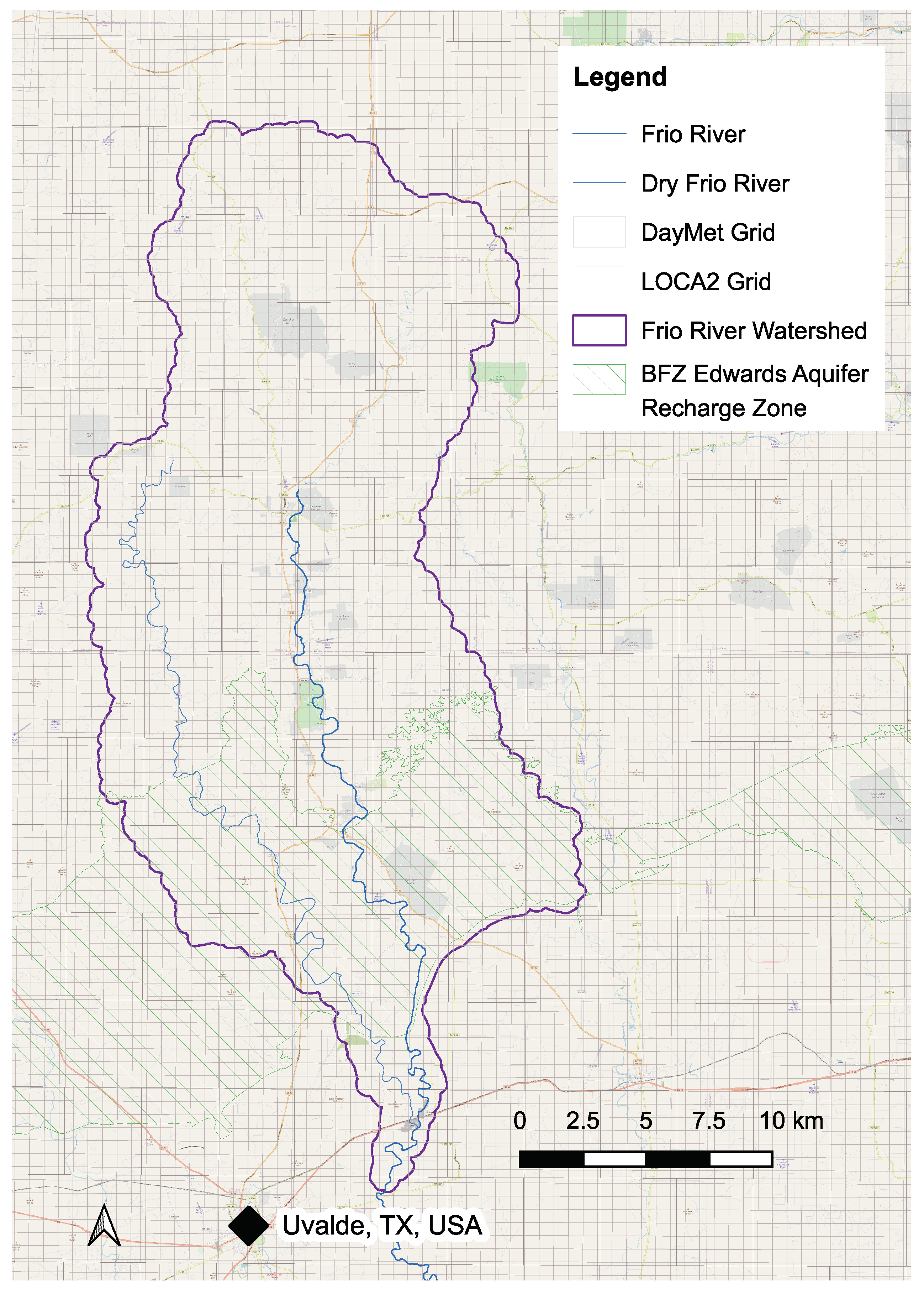
The study area was the Frio River basin in south-central Texas (TX), which is shown in Figure 1. This basin is about 134 km west of San Antonio, TX. The Frio basin is important from a water budgeting perspective because the Frio and Dry Frio Rivers cross the Balcones Fault Zone (BFZ) Edwards Aquifer Recharge Zone within the watershed. In the Recharge Zone, direct communication between surface water and subsurface storage is feasible and likely to occur due to the karstic nature of the Edwards Aquifer.
2.2. Weather Observations
Daily precipitation depth, maximum temperature, and minimum temperature observations were acquired for the study area, see Figure 1, for 1 January 1980 through 31 December 2022 from the Daymet version 4 repository [16,17]. Daymet provides long-term, continuous, gridded estimates of daily weather and climatology variables by interpolating and extrapolating ground-based observations through statistical modeling techniques [16].
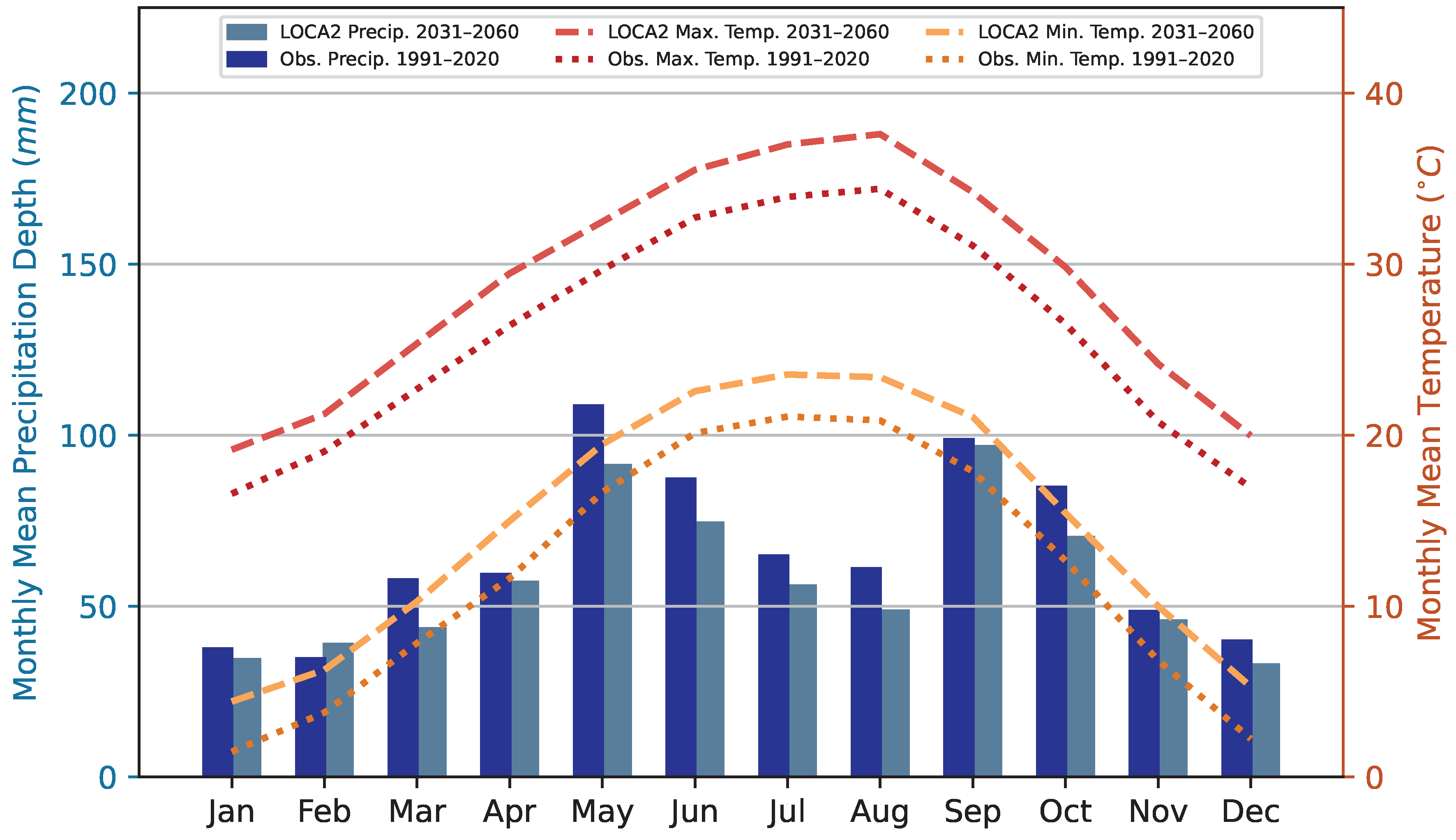
These datasets are available on a 1 km × 1 km spatial grid, which is displayed in Figure 1. Gridded estimates of daily weather are regionalized to provide a time series of daily weather parameters for the Frio basin. This regionalization is implemented using proportional area weighting, where grid cell values are weighted by the ratio of the grid cell area within the Frio basin to the entire area of the Frio basin. Monthly-averaged temperature and precipitation during 1991–2020 are presented in Figure 2.
2.3. Future Climate Projections
The Coupled Model Intercomparison Project (CMIP) is a foundational element of climate science because it coordinates the design and distribution of GCM simulations of the past, current, and future climate [18]. The most recent ensemble of CMIP-endorsed model intercomparison projects is Phase 6 or CMIP6. It contains 23 endorsed or approved GCMs [19].
Each CMIP6 model may be used to simulate one or more scenarios, as defined in the CMIP6 experimental design. In this study, the shared socioeconomic pathway (SSP) 5 with a 2100 radiative forcing level of 8.5 watts per square meter (W/m2) is the only CMIP6 scenario examined; this scenario is commonly labeled as ssp585. SSP5 represents a development path that is fossil-fueled and carbon emissions-intensive. It is predicated on the assumption of increasing integrated global markets, leading to innovations and technological progress. The social and economic development in this scenario is based on intensified exploitation of fossil fuel resources, characterized by a high percentage of coal usage and an energy-intensive lifestyle worldwide [20,21].
CMIP6 provides a collection of 23 global-scale climate simulation models. For application to a relatively small region like the Frio basin, as seen in Figure 1, the CMIP6 results need to be downscaled or interpolated to a more refined grid. CMIP6 results for the ssp585 scenario that were downscaled using the Localized Constructed Analogs version 2 (LOCA2) approach [22,23,24,25] were used for future climate projections. The LOCA2 grid configuration is shown in Figure 1.
LOCA2 statistical downscaling uses a 6-km resolution. The primary improvement of LOCA2, compared to the earlier version of LOCA, is in the representation of precipitation extremes [22,23]. LOCA2 downscaled CMIP6 ssp585 simulation results were obtained for daily maximum air temperature, daily minimum air temperature, and daily precipitation depth for the period from 1 January 2021 through 31 Decemebr 2065. The LOCA2 CMIP6 ssp585 results were regionalized to provide a unified time series of daily weather parameters for the Frio basin from each of the 23 CMIP6 models. This regionalization is implemented using proportional area weighting, where grid cell values are weighted by the ratio of the grid cell area within the Frio basin to the entire Frio basin area. Hereafter, “LOCA2” will refer to the ensemble of LOCA2 downscaled results from the 23 CMIP6 models for emissions scenario ssp585.
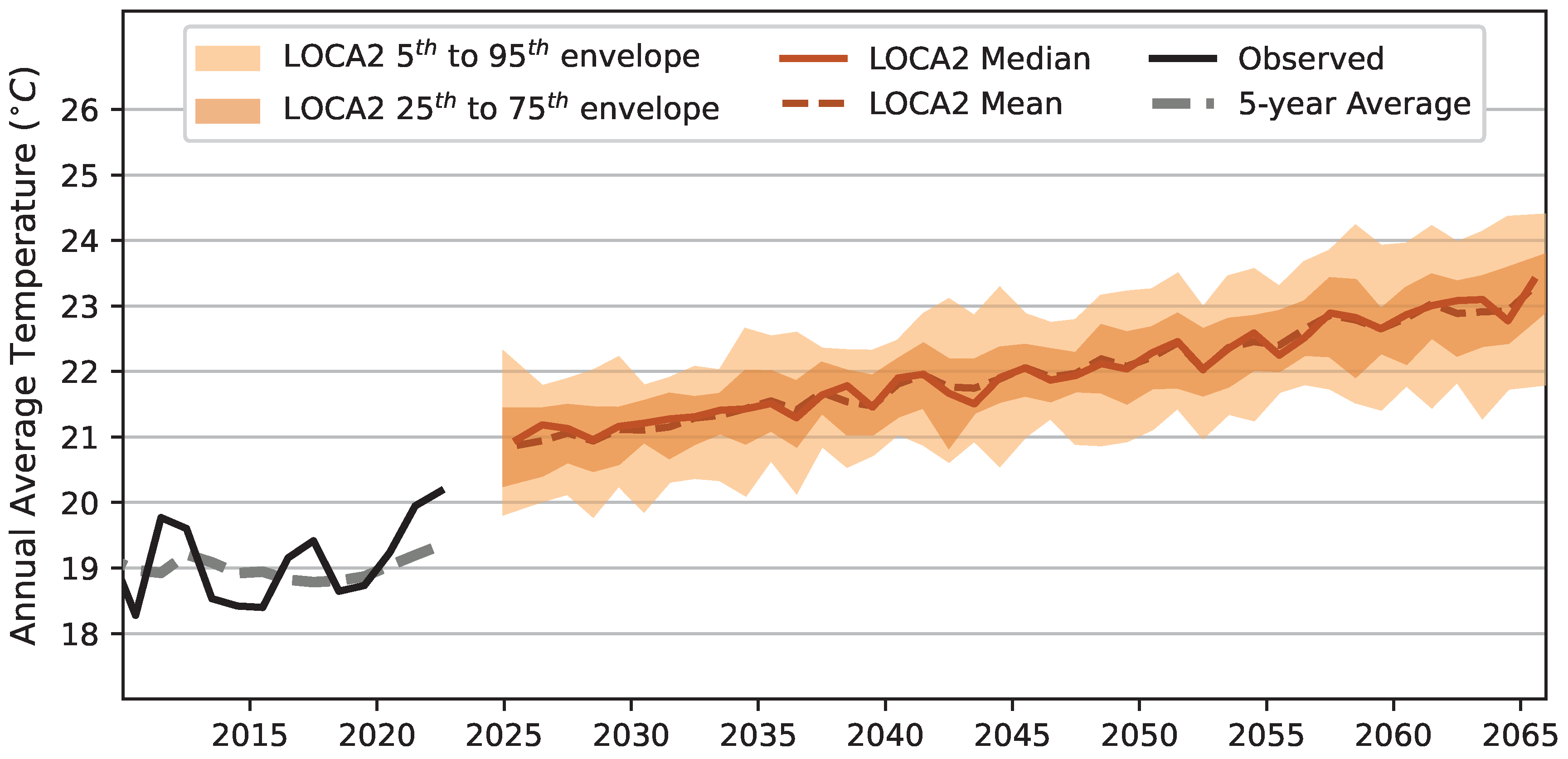
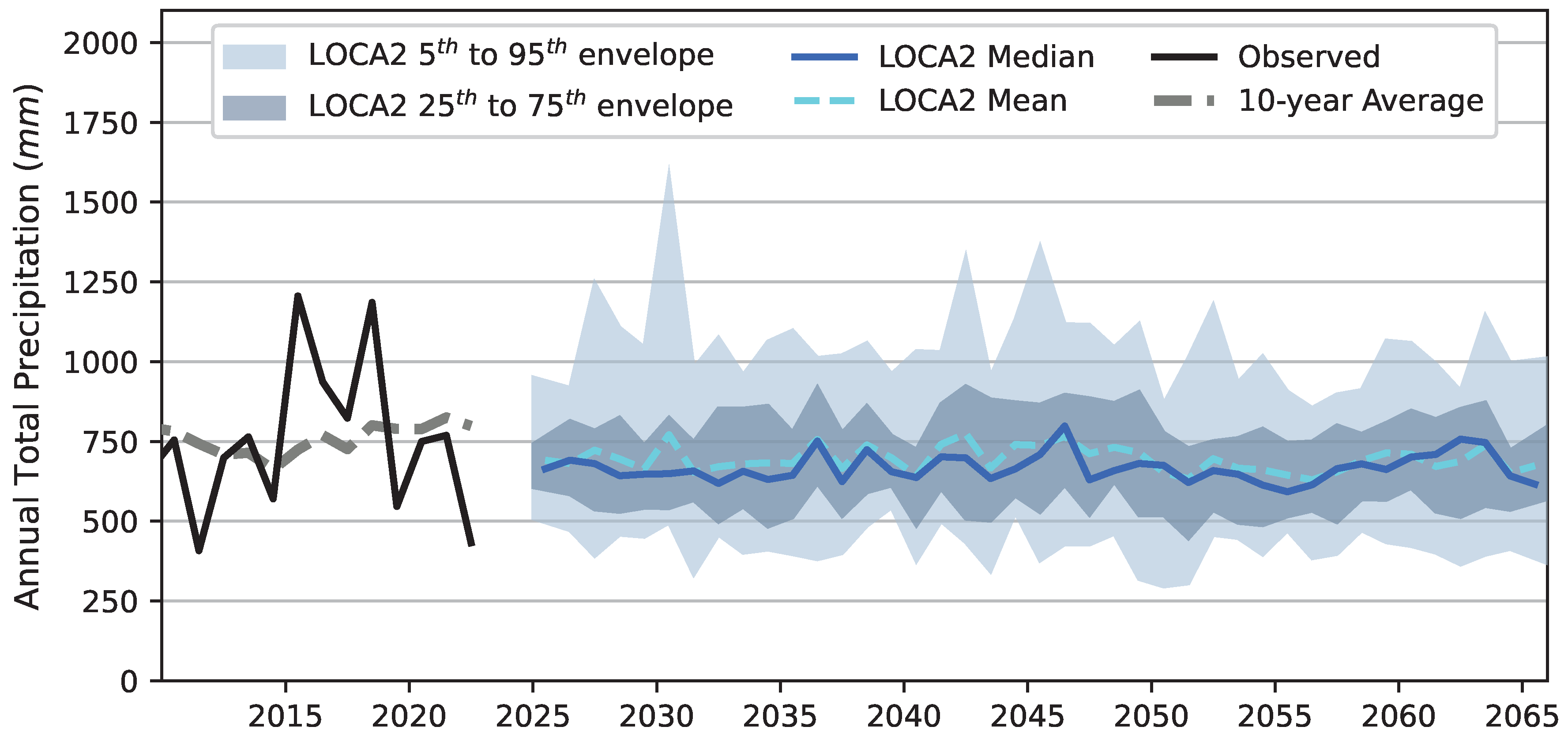
LOCA2 projected future climate is compared to the historically observed climate in Figure 2, Figure 3 and Figure 4. Figure 2 and Figure 3 show that temperature is expected to consistently increase in the future. Figure 2 and Figure 4 suggest that annual and seasonal precipitation depths will be similar, but decline slightly, for future conditions, relative to the historical observations.
2.4. Weather Attribution
Event attribution studies calculate if—and to what degree—a specific extreme event is made more likely or intense by climate change [1]. World Weather Attribution (WWA) refers to a collaboration of scientists from various organizations that have conducted numerous human-induced climate change attribution studies since the 2000s. The goal of WWA is to produce scientifically defensible attributions on short time scales following events with large impacts. WWA’s experience in attribution studies has led to the development of an eight-step procedure [26]: (1) analysis trigger, (2) event definition, (3) observational trend analysis, (4) climate model evaluation, (5) climate model analysis, (6) hazard synthesis, (7) analysis of trends in vulnerability and exposure, and (8) communication.
A detailed discussion of event attribution procedures is provided in Ref. [27]. Typically, the result of an attribution study takes the form of a probability ratio (PR). The PR is generally expressed as “the event has become X times more/less likely due to climate change with a 95% confidence interval of Y to Z”. The PR is often combined with an intensity impact summary, such as “the heat wave has become T (T1 to T2) degrees warmer due to climate change [26]”.
2.4.1. Summer 2022 Attribution Study
North America experienced an unusually warm summer in 2022, compared to prior observations, accompanied by abnormally dry soil conditions. High temperatures lead to increased land evapotranspiration and are, consequently, the main drivers of dry soil conditions. The WWA conducted an attribution study for the combined drought and heat wave in the summer of 2022. For the Northern Hemisphere extratropics, i.e., the region between the Tropic of Cancer (23.5° north of the equator) and the Arctic Circle (66.5° north of the equator), human-induced climate change made the observed soil moisture drought in June, July, and August of 2022 at least five times more likely for surface soil moisture, relative to the null hypothesis of no human-induced climate change [28].
To determine that the observed summer of 2022 surface soil moisture deficit was five times more likely to occur under human-induced climate change, Ref. [28] used three multi-model ensembles from different climate modeling experiments. One ensemble came from CMIP6, which used historical simulations from 1850 to 2015 compared to the ssp585 scenario for the 2016–2099 period. The second ensemble included the AM2.5C360 and FLOR high-resolution climate models developed at the Geophysical Fluid Dynamics Laboratory (GFDL). The HighResMIP SST-forced model ensemble, where SST stands for sea surface temperature, provided the third ensemble.
2.5. Drought Indexes
Drought is defined as “a deficiency of precipitation over an extended period of time (usually a season or more), resulting in a water shortage [29]”. Different types of droughts are sometimes labeled as meteorological and hydrological droughts. Meteorological drought refers to a period of extended precipitation deficiency. Hydrological drought refers to a period of extended low water supply [29].
Overallocation of resources to agricultural, domestic, and industrial consumption is at least as significant as precipitation deficiency in creating extended periods of low water supply. Overallocation is a widespread issue, often resulting from a combination of overly optimistic assessments of expected water resources and gross resource mismanagement [30,31]. This study focuses on weather and climate parameters, employing the standard definition of drought as an extended period of precipitation deficiency.
Drought indices are commonly used as probabilistic, statistical tools to identify drought severity and guide resource conservation and management. The probabilistic component of these indices is important because it allows for their use in risk and decision analysis [32]. Two different drought indexes are used: (1) standardized precipitation index (SPI) and (2) standardized precipitation evapotranspiration index (SPEI).
2.5.1. Standardized Precipitation Index (SPI)
SPI was developed to provide a better representation of abnormal wetness and dryness than previous indices. It is computed from a precipitation total over a pre-selected duration, like 3, 6, or 12 months [33,34]. The SPI is a probability-based index, designed to be a spatially invariant indicator of drought that acknowledges the importance of time scales in analyzing water availability and use. Essentially, it is a standardizing transform of the probability of observed precipitation [32], which is equivalent to the power transform algorithm used for the standardization of features and outcomes in machine learning [35].
The probabilistic component of the SPI involves fitting a probability distribution to collections of cumulative monthly precipitation totals for each year in a dataset. An SPI value is calculated for each month in the underlying precipitation dataset. Because the SPI is derived from a collection of annual values, it provides an intrinsic return period calculation. Table 1 presents SPI drought intensity definitions. Negative SPI values denote precipitation deficiency, i.e., drought, and positive SPI values denote precipitation excess. The sum of SPI values over consecutive months can be used as a drought magnitude index to compare different periods of historical drought periods [34].
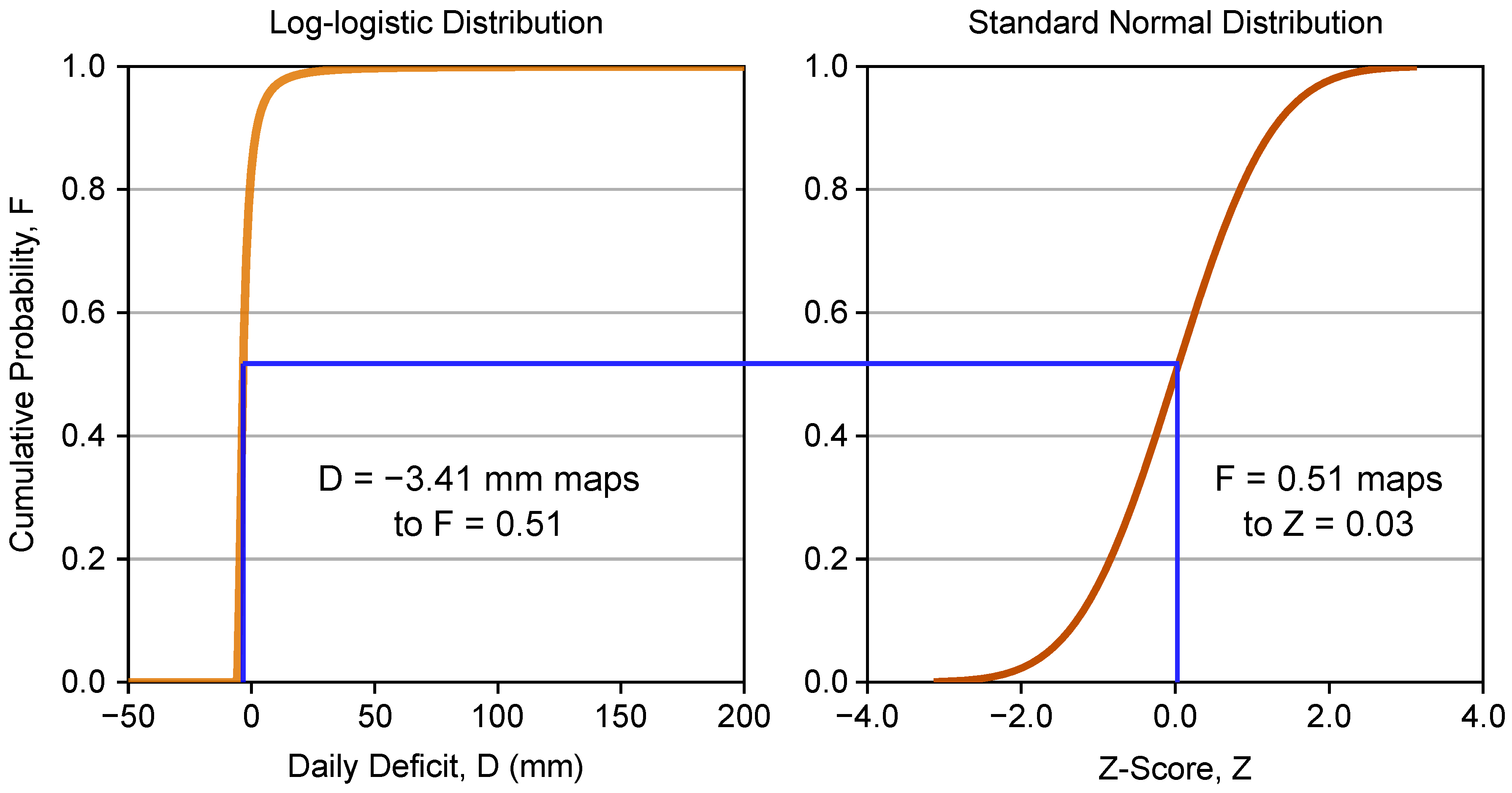
Figure 5 graphically demonstrates the standardizing transform that constitutes the SPI calculation. This figure shows the fitted distribution type for the SPEI; however, the SPI transform is identical to the SPEI transform. The SPEI uses deficit and a log-logistic distribution while the SPI uses precipitation and a gamma distribution. It should be noted that the implementation of the SPI in this work follows the approach of using the gamma distribution as per Refs. [33,34], rather than the Pearson type III distribution recommended by Ref. [32].
The calculation of the SPI is subject to the “problem of zeros”, where it is possible for the cumulative precipitation across 3- and 6-month intervals in the study area to be zero. This results in an undefined return period due to a cumulative probability, F, as shown in Figure 5, of zero. Cumulative precipitation must be greater than zero for the return period estimation. To address this issue, a minimum F value of is enforced. A gamma distribution is fit to the annual values across 1981–2010, which is 30 years. N denotes the number of years, and the minimum F value respects the maximum recurrence interval rule-of-thumb as outlined in Ref. [36].
2.5.2. Standardized Precipitation Evapotranspiration Index (SPEI)
The SPEI was developed to provide a climatic drought index that is sensitive to global warming. It is based on precipitation and temperature data, thus incorporating sensitivity to temperature increases and global warming considerations. The SPEI has the advantage of combining multiple parameters, providing the ability to include the effects of temperature variability on drought assessment [37].
The SPEI is congruent with the SPI, with the primary difference being the use of monthly water deficit (D) values in place of monthly precipitation (P) values. Equation (1) presents the definition of D where denotes potential evapotranspiration. in this study is calculated using the approach described in Appendix A.2.
The purpose of including in the drought index calculation is to obtain a relative estimation of time-varying dryness potential; consequently, the method used to calculate is not critical to SPEI implementation. “Temperature-only” estimates are generally used to provide a direct tie to global warming projections [37]. A positive D value denotes a monthly water surplus, and a negative D value identifies a monthly water deficit.
2.6. Using Drought Indexes with Weather Attribution
The standardizing transform integral to drought index determination assigns a probability value to each cumulative D for SPEI or cumulative P for SPI. Ref. [28] conducted a human-induced climate change attribution study for North America focusing on the drought during the summer of 2022. The study found that climate change made the observed soil moisture drought five times more likely, as discussed in Section 2.4.1. This attribution study, in conjunction with the SPEI calculated using the 1981–2010 Climate Normals, is used to establish targets for weather generator calibration through the following steps
- 1.
- Log-logistic distribution fit to 3-month cumulative D values from 1981–2010.
- 1981–2010 is within the historical period of 1850–2015 used in the attribution study.
- 2.
- Observed 3-month cumulative D transformed to SPEI using Figure 5 for 1993–2022 and the log-logistic distributions fit to the 1981–2010 observed values.
- The lowest SPEI identified from July and August 2022 has the target drought magnitude, and July 2022 for the Frio basin has the lowest SPEI.
- 3.
- The observed 3-month cumulative D for July 2022 SPEI provides the drought magnitude.
- Historical probability, F, of the July 2022 drought magnitude is determined as part of the SPEI calculation in item no. 2.
- 4.
- Historical July 2022 likelihood, F, is multiplied by 5 to obtain the target, human-induced climate change probability for the July 2022, 3-month cumulative D.
- The July 2022, 3-month cumulative, D, denotes the observed drought magnitude.
- denotes the “new” likelihood of the observed drought magnitude under human-induced climate change conditions.
2.7. Weather Generators (WGs)
A WG is a stochastic, statistical model of daily weather sequences. When a weather generator reproduces key statistical properties of meteorological records, it provides a concise distillation of the climate. WGs are commonly used in water resource planning and design, and agricultural, ecosystem, or climate change analysis applications because meteorological data may lack temporal or spatial coverage for the area of interest. WGs are not weather forecasting algorithms or deterministic weather models; consequently, it is not expected that a stochastically simulated weather sequence will be duplicated exactly by historical or future weather observations [9]. In the same way, it is not expected that weather sequences observed in the future will exactly duplicate historically observed weather sequences because the atmosphere provides an inherently chaotic system.
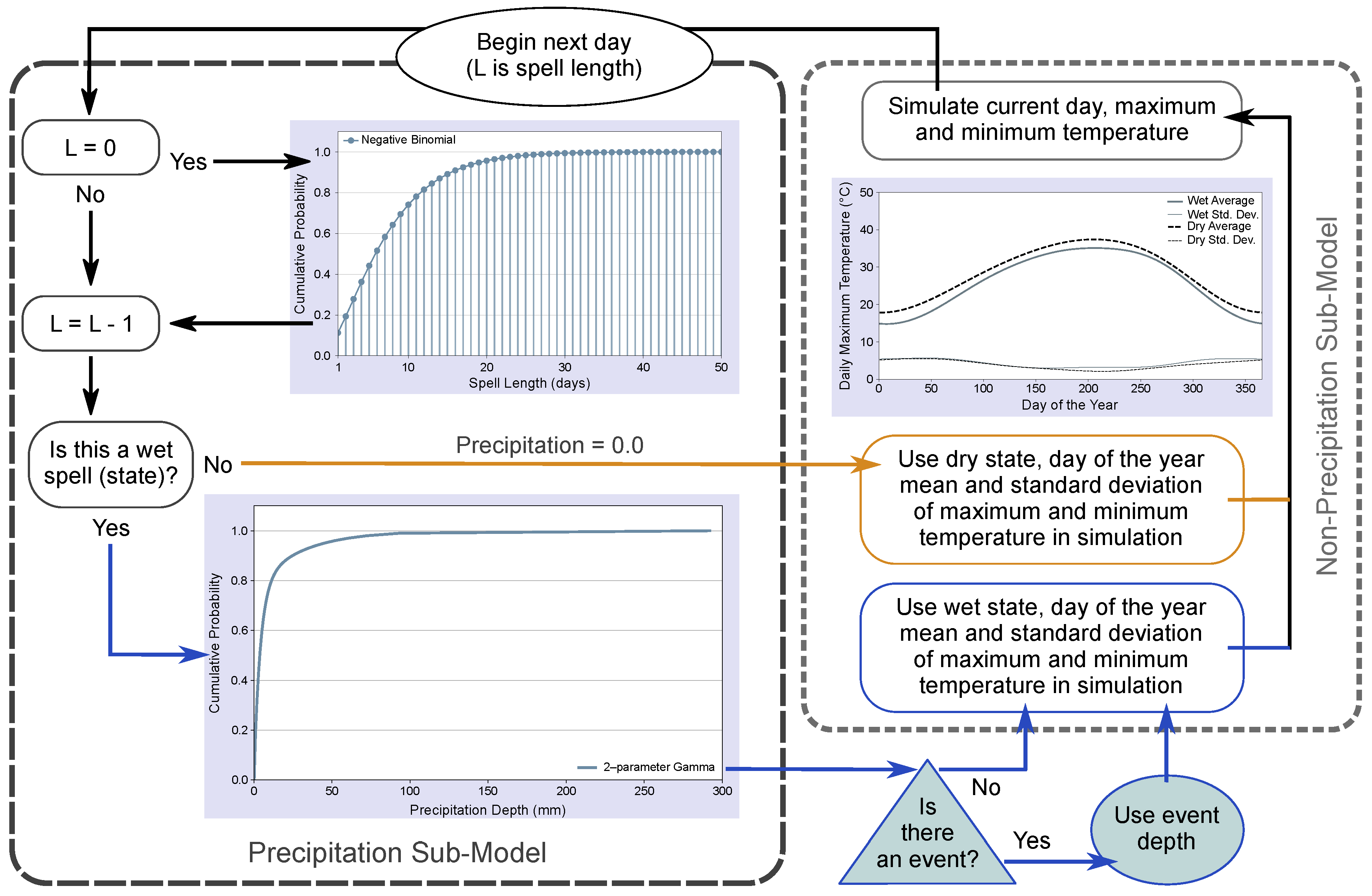
Daily precipitation depth, maximum air temperature, and minimum air temperature are stochastically simulated using a weather generator in this study. The simulation of precipitation depth includes the depiction of precipitation occurrence and intensity. Occurrence is represented by two states: (1) wet and (2) dry. In the dry state, precipitation depth is always zero. In the wet state, intensity, or daily precipitation depth, is stochastically simulated. Air temperature simulation is conditional upon the current state. Figure 6 provides a schematic showing weather generator formulation and operation.
2.7.1. Precipitation Occurrence with Spell Lengths
Alternating spell lengths are used to represent precipitation occurrence. The duration of a spell length for a state is sampled from a negative binomial distribution for that state. When the spell length duration has elapsed, a duration for the spell length of the other state is sampled from a negative binomial distribution for the new state. Every time a spell length elapses, the process is repeated, toggling to the other state for the selection of a new spell length, creating an alternating renewal process representation [9].
Negative binomial distributions are used to represent the spell-length likelihood and magnitude for both states and each month. This means that precipitation occurrence is represented by 24 (2 states × 12 months = 24) negative binomial distributions. The negative binomial probability distribution represents a discrete random variable. It describes a sequence of independent and identically distributed (i.i.d.) Bernoulli trials, repeated until a predefined, non-random number of successes occurs [38].
The negative binomial discrete random variable object from the SciPy stats library [38] is used in this study. It is defined using two shape parameters, N and P, and a location specification. N denotes the number of successes, and P denotes the probability of a single success [38]. N and P are the parameters for each of the 24 negative binomial distributions that are determined through calibration. The location parameter is set by the state. For wet-state distributions, a location parameter value of one is used, and a location parameter value of two is used for dry-state distributions.
2.7.2. Precipitation Intensity
The two-parameter gamma distribution provides precipitation intensity representation. A unique gamma distribution is used for each month, providing a total of 12 gamma distributions within the WG. The two-parameter gamma distribution is commonly used to represent precipitation intensity in weather generators [9].
A generalized form of the gamma probability distribution for a continuous random variable from the SciPy stats library [38] is used in this study. The generalized form accepts a location and scale parameter in addition to the two shape parameters, a and c. The scale, a, and c are the three parameters determined through calibration. The location is set to 0.255 mm for all gamma distributions and specifies the minimum precipitation intensity (0.255 mm/day) that can be simulated.
A truncation threshold is also used for each month to cap the maximum allowable daily precipitation depth estimated by the WG. This threshold is set to the 95th percentile daily precipitation depth observed for the month from 1991 to 2020.
2.7.3. Air Temperature
Other weather parameters, besides precipitation depth, have been simulated in WGs. Examples include temperature, solar radiation, and wind speed [39,40]. Here, the maximum and minimum daily temperatures are non-precipitation parameters.
The representation of maximum and minimum daily temperature is conditioned upon the precipitation state. Conditioning temperature on the presence or absence of precipitation serves as a simplistic proxy for unrepresented processes like cloud cover [41].
Air temperature is conditioned on the precipitation state and calculated during stochastic simulation using methods from the WGEN weather generator [39,40,42]. This approach for non-precipitation variables is based on a first-order vector autoregression, which requires that the statistics of the current day’s values are fully determined by the values on the previous day [9]. The conditional calculation for air temperature is presented in Appendix A.3.
One modification to the state-conditional temperature calculation described in Appendix A.3 is the inclusion of an additive scalar, C, for daily minimum and maximum air temperatures and for each state, as shown in Equation (2). The additive scalar term provides a simple means to uniformly increase stochastically simulated temperatures, and it is determined through calibration.
In Equation (2), subscript k denotes the index number that identifies non-precipitation weather variables. It ranges from 0 to 1, where 0 represents the daily maximum air temperature, and 1 represents the daily minimum air temperature. Subscript 0 in “” signifies the dry state and 1 in “” signifies the wet state. and in Equation (2) denote the mean and standard deviations, respectively. z denotes Z-scaled or normalized residual elements that provide white noise-type adjustments to calculated temperature values. Finally, t identifies the Julian daytime index, which goes from 1 to 365 for “standard” years and 1 to 366 for leap years.
2.7.4. Extreme Precipitation Events
Extreme precipitation events are expected to become more intense as average temperatures increase. Additionally, consistent temperature increases are expected to produce more frequent drought conditions [43]. An extreme event representation was included within the WG to statistically represent the contrasting impacts of consistent warming: (1) more intense and frequent droughts combined with (2) more intense extreme precipitation events.
Extreme events are included in the WG, as shown schematically in Figure 6. When an event is triggered, the event magnitude overwrites the next wet day precipitation depth. This formulation allows wet spell length distributions, see Section 2.7.1, and wet day precipitation depth distributions, see Section 2.7.2, to portray the expectation for more intense droughts while including more intense extreme precipitation through the extreme precipitation event representation.
An event formulation includes the timing and magnitude of the event. Event objects follow Poisson distributions for interarrival times, enabling a stochastic representation of the occurrence time. They also employ uniform distributions for event magnitude. The Poisson distribution for interarrival times is parameterized using the mean recurrence interval in years for the event. The uniform distribution, which determines event magnitude, is parameterized with lower and upper magnitude bounds. The lower boundary is set at the current estimated event depth for the basin centroid for the average recurrence interval, as per Ref. [44], which is NOAA Atlas 14. The upper boundary magnitude is a calibration parameter. Table 2 outlines the extreme event configuration for calibration, along with 24-h point precipitation depth estimates from Ref. [44].
2.8. Calibration
The automated calibration or training was implemented with PEST, which stands for “parameter estimation” [45,46]. Parameter estimation with PEST employs an inverse-style approach where model parameters are estimated by varying parameter values to find values that produce the “best-fit” between simulated values and target observations. PEST provides data assimilation (DA) that seeks to combine information from model simulations with observations to obtain the “best” description of a system along with an accompanying description of uncertainty. Consequently, PEST really provides “calibration-constrained uncertainty analysis” rather than just “parameter estimation” [45].
The parameters, for which PEST seeks optimal values in this study, are mostly definition parameters for the probability distributions that comprise the WG, as discussed in Section 2.7. Appendix A.4 provides calibration parameters along with the ranges of values examined. Target observations are derived from the SPEI and weather attribution analyses; they are discussed in Section 3.1 and summarized in Appendix A.4.
3. Results
A weather attribution study is used to develop the target outcomes for WG training. A WG is then calibrated to simulate the best-fit outcomes and applied to produce weather attribution-guided future climate projections for the Frio basin.
3.1. Drought Targets from Weather Attribution
Target drought magnitude and likelihood, given human-induced climate change, are developed according to the procedures outlined in Section 2.6. The observed 3-month cumulative D for July 2022 is mm, which serves as the target drought magnitude for July. A historical SPEI of for July 2022, with an associated cumulative probability, F, of , is determined using a log-logistic distribution. This distribution is fit to the collection of 30 observed July 3-month cumulative D values from 1981 to 2010.
As noted in Section 2.6, July 2022 provides the lowest SPEI and 3-month cumulative D from the June, July, and August 2022 periods examined in the attribution study. Table 3 SPEI- and SPI-related values from May to September 2022. There was some precipitation, P, in August 2022, as indicated by the August 2022 3-month P and SPI values, which broke the severe drought earlier in this localized region than what was experienced across the majority of the Northern Hemisphere extratropics.
The target likelihood for the observed July magnitude of mm is five times the historical likelihood [28], or . This drought likelihood analysis under human-induced climate change is extended to the other calendar months by extracting the 3-month cumulative D for each month corresponding to a cumulative probability of . The extracted, cumulative D denotes the drought magnitude target for each month. The corresponding cumulative probability target for each month is then . Table 4 provides the drought magnitude and likelihood targets for each month.
3.2. Weather Generator Calibration
The purpose of calibration is parameter estimation. Optimal parameter values are those that produce the closest match between simulated values and target observations. Parameters, which are varied as part of calibration, are listed in Table A1, Table A2, Table A3, Table A4 and Table A5, along with the “optimal” or final parameter values. Target observations are described in Table A6. Best-fit simulated target values are provided in Table A6 and Table 4.
The annual average precipitation depth, P, was used as a target observation in addition to the monthly drought likelihood and magnitude values. Simulated annual average climate parameters from 2031 to 2060—from the calibrated WG—are compared to the historical observations from 1991 to 2020 and LOCA2 projected values from 2031 to 2060, as seen in Table 5.
3.3. Attribution-Constrained Future Climate Projections
The calibrated WG was used to make future climate projections from 1 January 2024 to 31 December 2065. A total of 1000 stochastic realizations of daily weather are used to generate the future climate description. The weather generator (WG) 2031–2060 future climate description is compared to the LOCA2 2031–2060 future climate description and the observed 1991–2020 climate description. Table 5 provides a comparison of the annual average P, , and D.
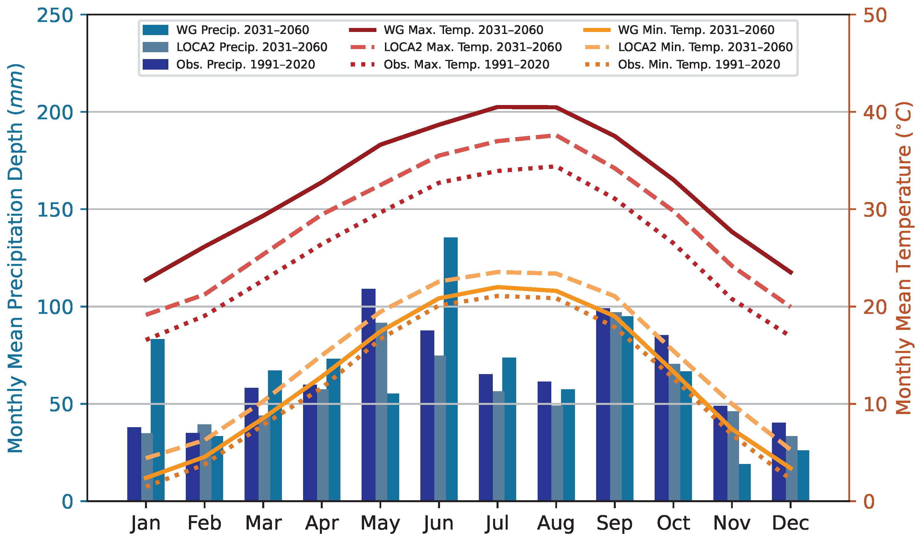
Figure 7 compares the monthly-average P, monthly-average daily maximum temperature, and monthly-average daily minimum temperature among WG 2031–2060 projected values, LOCA2 2031–2060 projected values, and 1991–2020 observed values. The attribution-constrained WG produces consistently warmer daily maximum temperatures and consistently cooler daily minimum temperatures than the LOCA2 2031–2060 values.
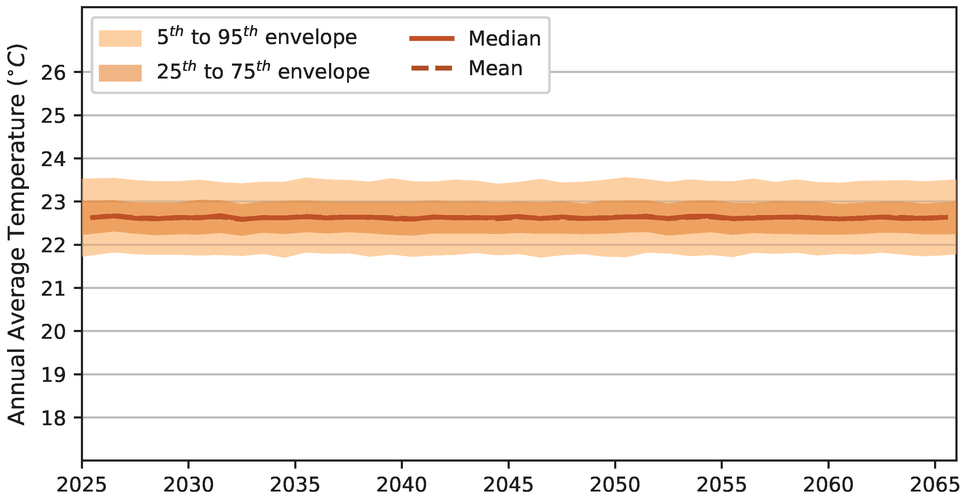
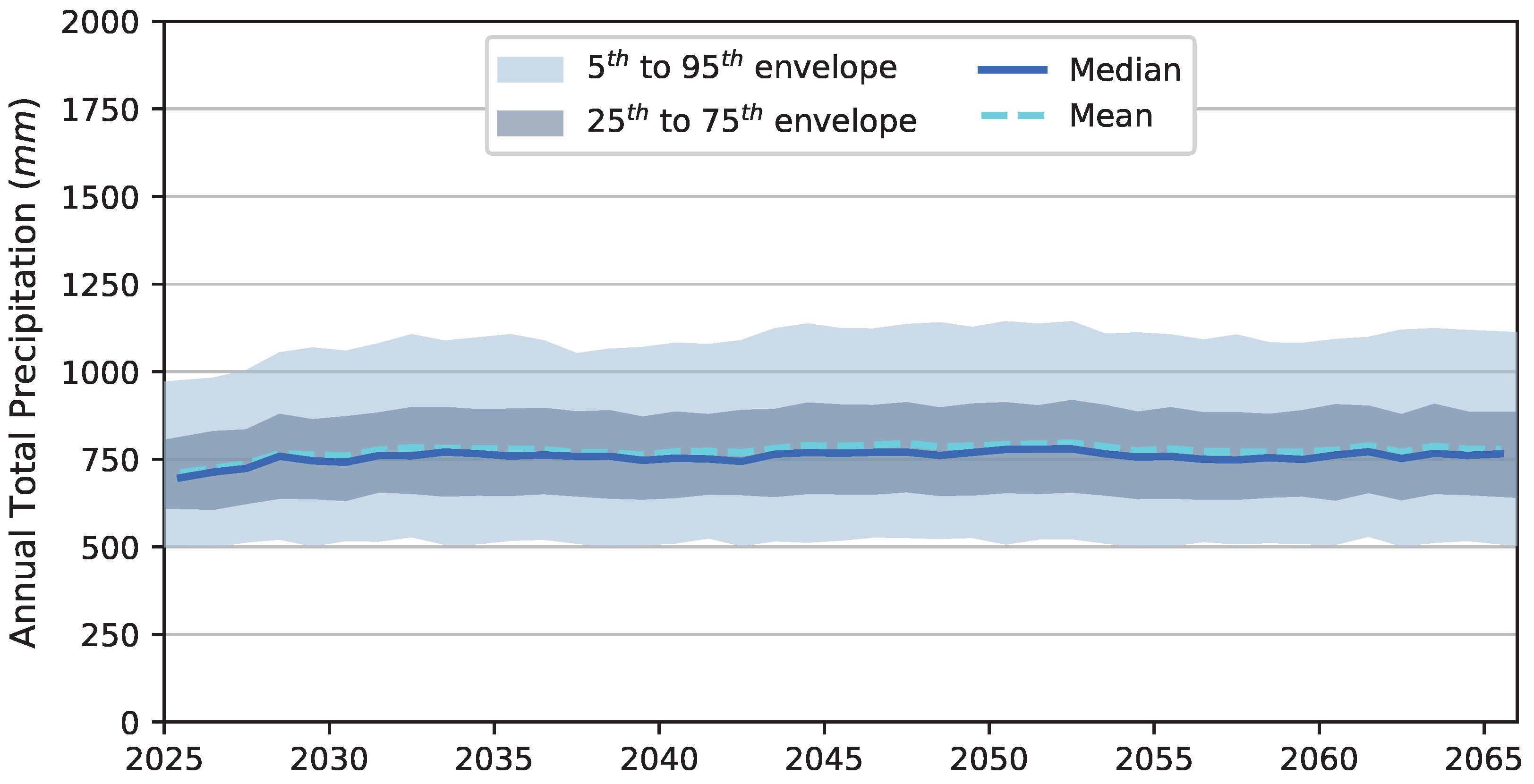
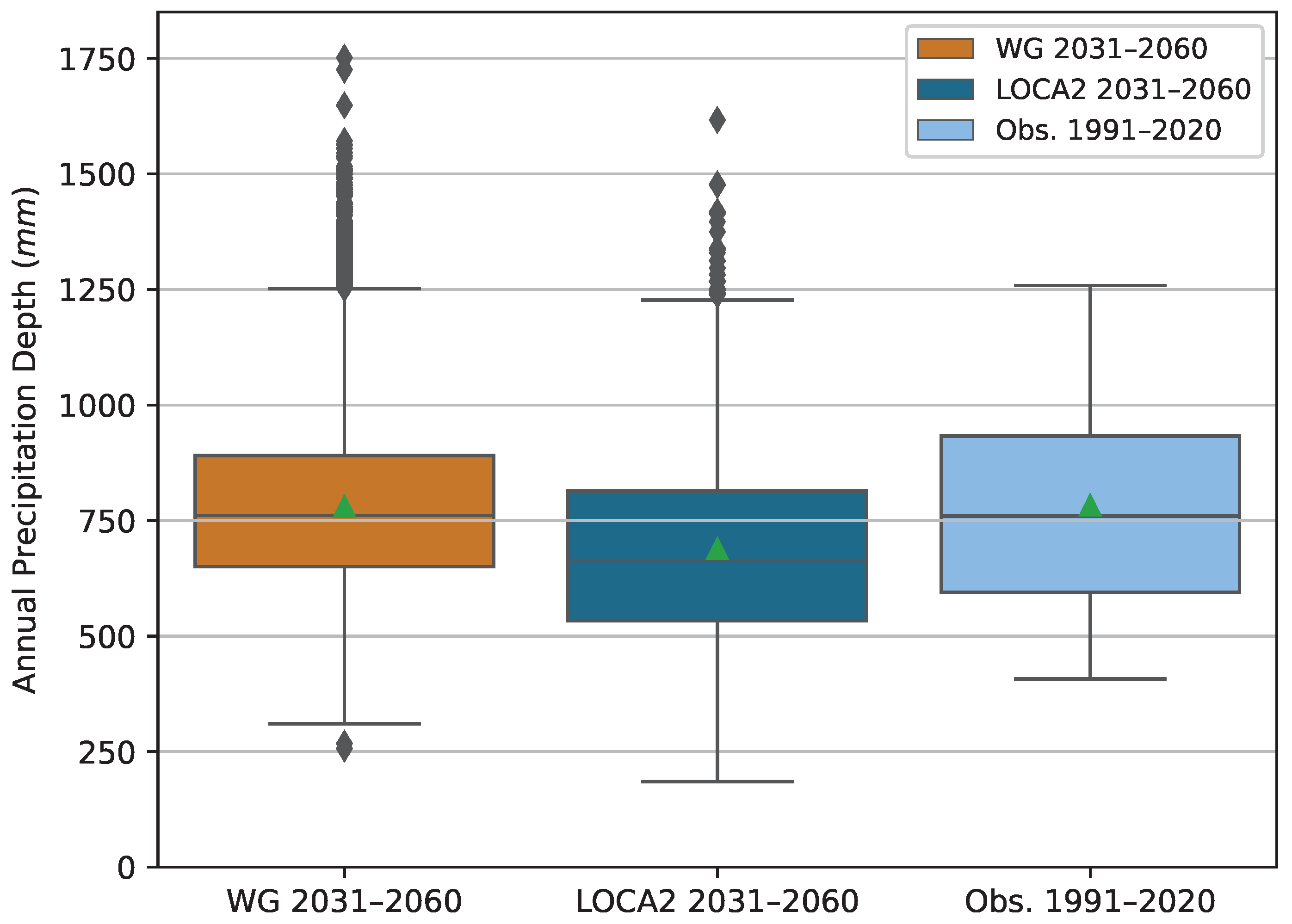
Figure 8 presents the WG-projected annual average temperature cone of uncertainty. In this case, the cone of uncertainty is flat because the WG formulation is stationary in time. Figure 9 displays the WG-projected annual precipitation depth cone of uncertainty. The distribution of annual precipitation depth is compared in Figure 10 among WG 2031–2060 projected values, LOCA2 2031–2060 projected values, and 1991–2020 observed values. The WG 2031–2060 mean annual P is approximately equal to the observed 1991–2020 mean annual P. LOCA2 projects a smaller mean annual P than the other two datasets.
Drought Conditions
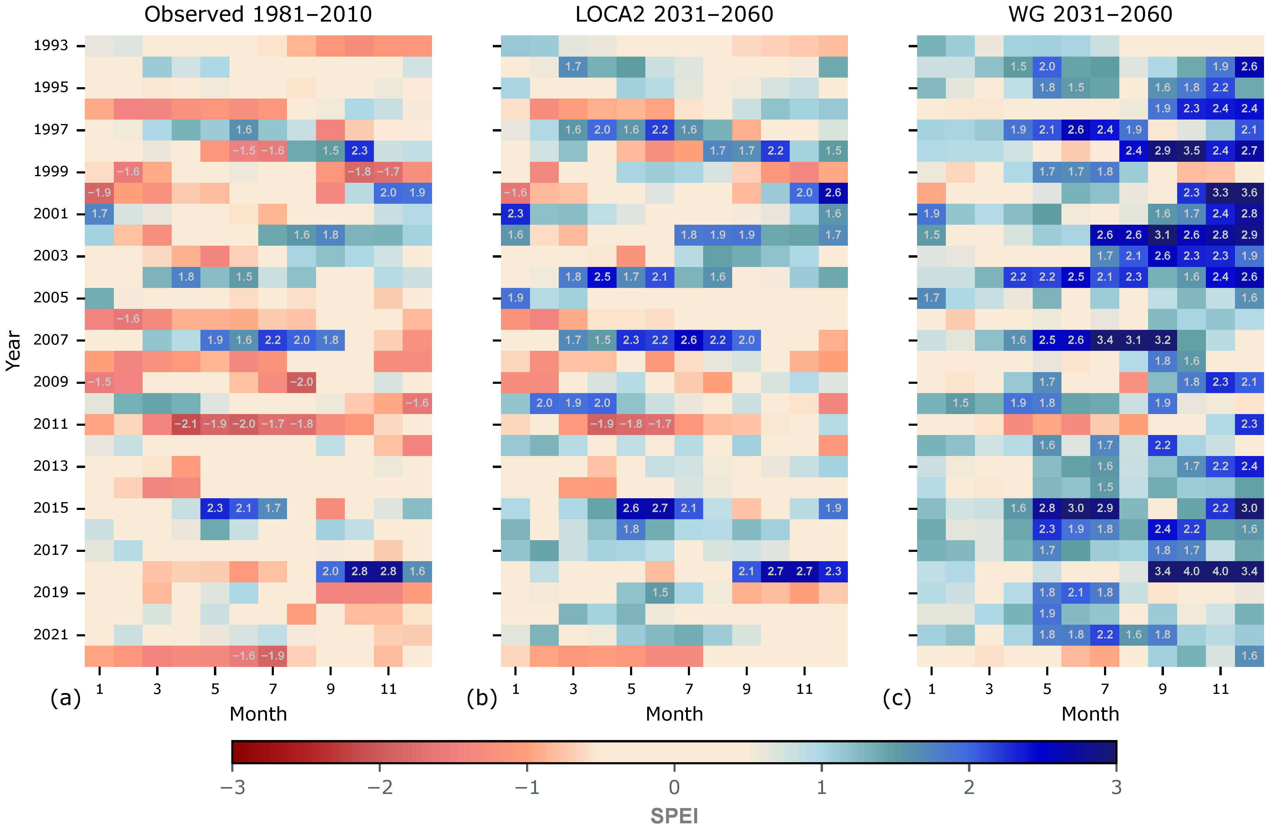
The WG is calibrated or trained to portray a drought magnitude, which has a recurrence interval of approximately 33 years () under historical 1981–2010 conditions, with a recurrence interval of approximately seven years () for future projected conditions. The cumulative 3-month D is used to define a drought magnitude, as shown in Table 4.
The observed 3-month D from 1993 to 2022 is used in Figure 11 to compare the relative drought conditions among the observed 1981–2010, LOCA2 projected 2031–2060, and WG-projected 2031–2060 conditions. When 1993–2022 observations are analyzed from the perspective of the WG 2031–2060 climate, there are no severe drought periods during the 1993–2022 period. A severe drought has an SPEI of 1.5 from Table 1. Figure 11 demonstrates that the WG 2031–2060 climate is significantly warmer and drier than the LOCA2 2031–2060 climate and the observed 1981–2010 climate.
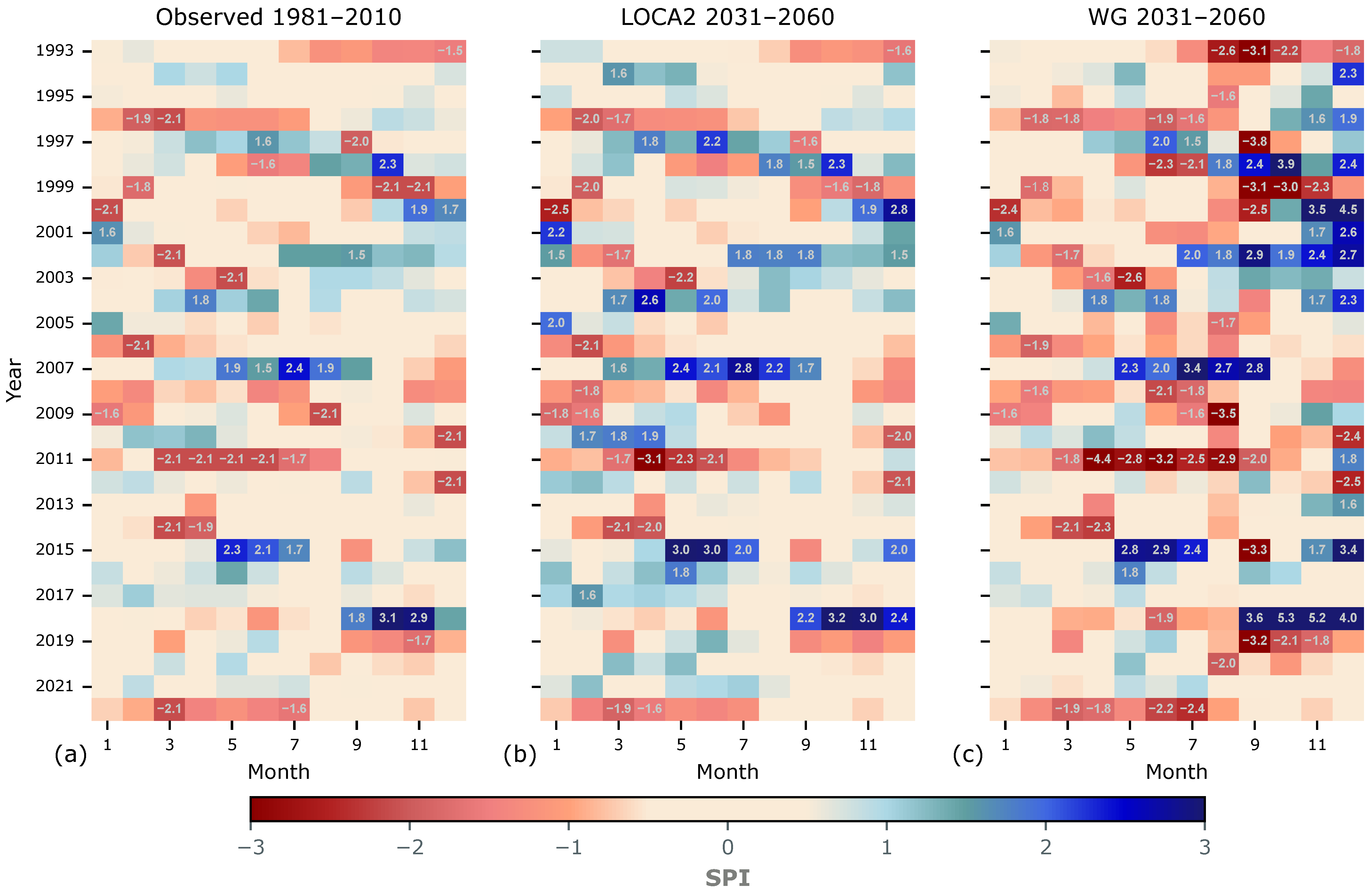
The observed P from 1993 to 2022 is used in Figure 12 to compare SPI-derived relative drought and wetness conditions among the observed 1981–2010, LOCA2 projected 2031–2060, and WG-projected 2031–2060 conditions. SPI depends only on P. Figure 10 shows that the annual average P values are approximately equal for the WG-projected 2031–2060 and observed 1991–2020 conditions and that the annual average P is expected to be smaller for the LOCA2 projected 2031–2060 conditions. Additionally, the WG-projected 2031–2060 conditions have the most large and small outliers, denoting an increased expectation for extreme events while maintaining a constant annual average P from the observed 1991–2020 conditions. Comparative results in Figure 12 agree with the comparisons among WG, LOCA2, and observed conditions in Figure 7 and Figure 10.
4. Discussion
CMIP6 simulations offer stochastic, day-to-day weather that is derived from a robust physical representation of future climate, based on idealized initial conditions and forcing scenarios. CMIP6 models represent the physics and physical processes in the atmospheric system. From the viewpoint of stochastic simulation, CMIP6 results provide stochastic day-to-day weather, sampled from the governing or underlying “climate” process, as well as a physics-based description of the “climate” process and its functions under varying initial and forcing conditions.
Stochastic WGs produce stochastic day-to-day weather, which is sampled from an underlying stochastic “climate” process that is specified when the WG is formulated. The underlying “climate” process is primarily specified through configuration and parameterization of the probability distributions that comprise the WG, as shown in Figure 6. For WG, the underlying “climate” process is external to the WG and must be derived or depicted based on other sources of information.
CMIP models are clearly superior to WGs in many cases because they provide stochastic day-to-day weather sampled from the underlying “climate” process and the physics-based description and representation of the “climate” process. A WG can only provide stochastic day-to-day weather sampled from an externally specified “climate” process. One scenario for which WGs provide additional utility relative to CMIP models is the case where the “climate” process has been described from other sources and datasets and is different in some manner from the “climate” process representation provided by CMIP models. An example of this scenario is the representation of extreme events.
Extreme events fall within the tails of the long-term aggregated description of weather that constitutes climate. A climate description can provide a probability for the occurrence of a generic event magnitude. However, for analyzing the likelihood of a regional-scale event, CMIP models alone are insufficient, as they are global in scale. In such analyses, CMIP simulation results are often augmented with other information sources, such as high-resolution, regional geophysical models and sea surface temperature models.
An observed event is weather, not climate. Weather attribution is a formalized and scientific approach used to identify the change in likelihood or PR for an observed event under two different climate regimes. Attribution provides the “new” or future probability of occurrence for event magnitude. Weather attribution is used in this study to generate drought magnitude and likelihood targets for WG calibration, and attribution provides the “climate” process description that is different from that contained within CMIP results.
Two advantages to using WGs are: (1) WGs can represent a “climate” process that is different from that represented in CMIP results and (2) WGs can easily produce large numbers of stochastic realizations, i.e., tens to hundreds of thousands. A large number of realizations is required to ensure robust sampling of the stochastic weather forcing input variables to a water balance model for every model input time in a water balance model. If biased forcing, resulting from the use of too few realizations, is propagated through a water balance model, then the resulting water budget estimates will also be biased.
As an example of the importance of robust sampling, the 95th percentile time history in Figure 4 shows a peak of about 1750 mm in 2030. This is not a future prediction contained within the LOCA2 results for the increased likelihood of a very wet year in 2030. The occurrence of a wet year in 2030 is a weather event and is only evident in Figure 4 because 23 stochastic realizations of day-to-day weather are employed to generate the figure.
A climate description used for the forcing of a water budget model should provide approximately the same likelihood for an annual precipitation depth value for every year between 2030 and 2040. In Figure 9, the 95th percentile time history ranges between 1048 and 1102 mm between 2030 and 2040. A total of 1000 stochastic realizations were used to produce Figure 9; the 95th percentile time history is not as flat as would be necessary to indicate the same likelihood for an annual precipitation depth of about 1075 mm for each year between 2030 and 2040. As the number of stochastic realizations of day-to-day weather increases, probabilistic time histories, such as the 95th percentile, will become flatter within an interval of assumed stationarity.
Time stationarity is the assumption that time series statistical properties do not change across an interval. Strict stationarity is generally too restrictive, and a reduced requirement, called weak stationarity, is often used. Weak stationarity imposes restrictions on the first two statistical moments of the time series; it formally requires a constant mean and an autocovariance function that depends only on the time difference or lag and is independent of the specific points in time that are differenced [47,48]. The WG formulation presented in Figure 6 enforces strict stationarity across the simulation interval because the probability distributions that comprise the WG are defined in generalized form, requiring three to four parameters, and the parameters that define the probability distributions are held constant across the simulation interval.
Two disadvantages of using WGs relative to CMIP results are: (1) WGs are purely statistical and probabilistic, relying on robust sampling to produce a meaningful climate description, and (2) WGs inherently require the assumption of time stationarity and cannot represent the physics-based evolution of process functions to produce trends. An example of the first shortcoming can be seen in Figure 7, where the structure of the calculation employed in this study pushes the calibrated WG daily maximum and minimum temperatures apart in order to increase the calculated to meet the constraint of the drought targets. The LOCA2 results in Figure 7 suggest a more likely future climate description, where both maximum and minimum temperatures increase uniformly and there is relatively constant increase in the projected future temperature. An example of the second shortcoming is presented in Figure 8, where the calibrated WG simulated annual average temperature is relatively flat or constant across the simulation interval. An improved representation is provided in Figure 3, where there is a trend of an increasing average annual temperature across the analysis interval. One approach that can be implemented with WGs to partially represent trends is to use several intervals of assumed stationarity to reproduce the trend in a step-wise fashion [7,8].
Stochastic simulation is a system simulation that uses variables that can change randomly with individual probabilities for each variable [49,50]. When an ensemble of stochastic realizations of day-to-day weather is used for input water budget model forcing, then the water budget simulation framework is stochastic. When observed weather forcing is used for input water budget model forcing and resulting water budget calculation outputs are compared to observations, like in traditional model calibration, the water budget simulation framework is deterministic. For both types of inputs (stochastic and observed), the water budget model itself, in contrast to the simulation framework, is deterministic if it always produces the same results for the same inputs.
For stochastic simulation, the sampling of variables, which change randomly with individual probability distributions, directly controls the quality of the results obtained. Sampling bias is an error in estimates or simulation results due to a sampling procedure that is not representative of the underlying population described by the probability distribution [51]. In many cases, the sampling of the stochastic inputs is more important than the deterministic water budget model used to propagate uncertainty from stochastic inputs to estimates or outputs.
When stochastic inputs or variables are used and the water budget modeling framework is stochastic, simulation results must be presented probabilistically with cones of uncertainty, similar to what is done in Figure 8 and Figure 9, or as long–term ensemble averages, as done with the Climate Normals in Figure 7. The simulation results for a single outcome realization always present sampling bias because a single outcome realization is derived from a single input forcing sample.
Future Work
WG formulation in this study focuses on reproducing attribution study likelihoods and historically observed annual average precipitation depth. CMIP6 ssp585 simulation results are used in the attribution study to determine the change in likelihood but are not directly employed as targets for WG training.
Future work will examine explicitly combining CMIP simulation results and weather attribution to generate a comprehensive set of targets for WG calibration. Specifically, it would be interesting to use the annual average precipitation depth and 2031–2060 average monthly precipitation depths, see Figure 7, from the LOCA2 2031–2060 climate description, in addition to the drought likelihood and magnitude values, see Table 4, as calibration targets.
5. Conclusions
Weather attribution provides drought magnitude and likelihood targets for WG calibration. Drought conditions of the magnitude observed for the study area during June, July, and August 2022 are expected to be five times more likely to occur under human-induced climate change conditions relative to the historical conditions. A WG is calibrated for the study area to approximately reproduce the five-time increase in probability for historically severe droughts. The 2031–2060 climate description produced by the calibrated WG is significantly hotter and has lower expected soil moisture compared to the 2031–2060 climate description obtained from LOCA2 simulation results.
Projected future day-to-day weather provides stochastic forcing when used to generate water balance model projected outcomes. A WG that is calibrated to reproduce observed weather event magnitude and likelihood for a “new” or different climate regime, such as human-induced climate change relative to pre-industrial conditions, offers an alternative to the climate description provided by GCM simulation results. The attribution-constrained WG future climate description can portray more extreme conditions and events than those obtainable from a global-scale model driven by idealized forcing and initial conditions.
Funding
This research was funded by the Edwards Aquifer Authority (EAA) under contract 23-020L-AMS.
Institutional Review Board Statement
Not applicable.
Data Availability Statement
The weather generator produced data presented in this study are available from the project GitHub per Appendix A.1. The weather generator produced data sets are the only new data created and analyzed in this study.
Acknowledgments
Andrew Kazal from ICF extracted the LOCA2 datasets from public repositories and clipped them to the study area, simplifying the analysis of these datasets. The author wishes to acknowledge the contributions of the four anonymous reviewers whose comments and suggestions improved the quality of this paper.
Conflicts of Interest
The funding sponsors had no role in the design of the study; in the collection, analyses, or interpretation of data; in the writing of the manuscript, and in the decision to publish the results. The author declares no conflict of interest.
Abbreviations
The following abbreviations are used in this manuscript:
| AET | actual evapotranspiration |
| BFZ | Balcones Fault Zone |
| CMIP | coupled model intercomparison project |
| DA | data assimilation |
| EAA | Edwards Aquifer Authority |
| ET | evapotranspiration |
| GCM | global climate model |
| HS85 | Hargreaves–Samani 1985 equation for |
| iid | independent and identically distributed |
| LOCA2 | localized constructed analogs version 2 |
| PET | potential evapotranspiration |
| PR | probability ratio |
| SPEI | standardized precipitation evapotranspiration index |
| SPI | standardized precipitation index |
| SSP | shared socioeconomic pathway |
| WG | stochastic weather generator |
| WWA | World Weather Attribution |
Appendix A
Appendix A.1. Source Code Availability
The “New” weather generator source code and associated calibration files are available online from the project GitHub repository at:
https://github.com/nmartin198/wattrib_wg_frio (accessed on 10 October 2023)
Appendix A.2. Potential Evapotranspiration (PET) Calculation
Evapotranspiration (ET) is typically the primary way water is subtracted from a watershed. It includes water loss from the leaves of plants, known as transpiration, and water that evaporates from the soil surface, puddles, ponds, lakes, and rivers. Transpiration and evaporation are usually considered together as ET at the watershed scale. ET dominates the water balance and controls the availability of water for soil moisture storage, groundwater recharge, and runoff. denotes the rate of water loss to the atmosphere when not limited by water supply. In contrast, actual evapotranspiration (AET) is the actual rate of water loss to the atmosphere, constrained by the amount of water available from precipitation and irrigation [5].
Precipitation and temperature are the historical, observed, and future projected weather parameters for this study. is estimated using temperature, as it is the available weather parameter for the calculation, along with expected solar radiation, which is based on the study area’s latitude and season.
can be estimated from the reference crop evapotranspiration, , using a crop coefficient, , as shown in Equation (A1). In this study, and , so the calculated future is primarily dependent on the projected future temperature.
A modified version of the Hargreaves–Samani 1985 (HS85) equation [52,53] from Ref. [54] is used to estimate , with Equation (A2), from the daily average temperature, , calculated using Equation (A3). Equation (A2) is the modified version of the HS85 equation, and the modification involves the use of the monthly-average difference in the daily maximum and minimum temperatures rather than the annual difference.
Equation (A2) provides the reference crop evapotranspiration, , in millimeters per day. In this equation, represents the water equivalent of extraterrestrial radiation in millimeters per day. denotes the difference between the monthly-average daily maximum temperature, , and the monthly-average daily minimum temperature, , as shown in Equation (A4). All temperature values in these equations are in degrees Celsius.
denotes the daily maximum temperature, and denotes the daily minimum temperature.
The water equivalent of extraterrestrial radiation in millimeters per day, , is calculated using Equation (A5), where denotes the relative distance between the earth and the Sun, as derived from Equation (A6), denotes the sunset hour angle in radians using Equation (A7), denotes the site latitude in radians, and denotes the solar declination in radians from Equation (A8).
J denotes the Julian day number.
Appendix A.3. Conditional Temperature Formulation
In the weather generators used in this study, air temperature is calculated as conditional upon the precipitation state. This conditional formulation is presented in Equations (A9)–(A14). The day of the year mean, , and standard deviation, , in Equation (A9) for each state were determined using Fourier series smoothing—or low-pass filtering—of the day of the year mean and standard deviation series derived from data. The smoothed mean series was subtracted from the original data series, and the smoothed standard deviation series was used to normalize the result to produce Z-scaled residual elements, . Residual elements are used to calculate , Equation (A13), and , Equation (A14), matrices which are used to calculate the A, Equation (A11), and B, Equation (A12), matrices [40,42].
t denotes the Julian daytime index. k denotes the index for the number of non-precipitation weather variables. denotes a dry-state non-precipitation weather variable, and 0 signifies the dry state. denotes a wet-state non-precipitation weather variable, and 1 signifies the wet state.
signifies a k-dimensional vector of independent standard normal variables that provides white-noise forcing for each variable.
denotes the lag 0 covariance matrix from Equation (A13), and denotes the lag 1 covariance matrix from Equation (A14).
denotes the lag 0 cross-correlation coefficient between variables.
denotes the lag 1 cross-correlation coefficient between variables.
Appendix A.4. Calibration Parameters
A total of 94 parameters are adjusted during calibration: 4 parameters are additive scalar temperature factors, as per Table A1; 6 parameters define the upper bounds for extreme event magnitudes in Table A2; 24 parameters (12 months × 2 parameters) determine the dry-state spell length distributions, detailed in Table A3; another 24 parameters 12 months × 2 parameters) are for wet-state spell length distributions, as shown in Table A4. Additionally, 36 parameters (12 months × 3 parameters) are set for precipitation intensity distributions, as seen in Table A5.
Moreover, 13 observations are used for targets, as shown in Table A6.

Table A1.
Additive scalar temperature parameter specifications for calibration and “best-fit” values.
Table A1.
Additive scalar temperature parameter specifications for calibration and “best-fit” values.
| Parameter Name | Description | Transform | Change Limit | Initial Value | Lower Bound | Upper Bound | Group | Calibrated |
|---|---|---|---|---|---|---|---|---|
| parnme | partrans | parchglim | parval1 | parlbnd | parubnd | pargp | Final Value | |
| tmax_wet_add | Equation (2) | log | factor | 5.1 | 2.0 | 8.0 | temp | 5.1 |
| tmax_dry_add | Equation (2) | log | factor | 6.1 | 2.0 | 8.0 | temp | 6.9 |
| tmin_wet_add | Equation (2) | log | factor | 0.9 | 0.1 | 3.0 | temp | 0.9 |
| tmin_dry_add | Equation (2) | log | factor | 0.9 | 0.1 | 3.0 | temp | 0.8 |
Table A2.
Extreme event scalar temperature parameter specifications for calibration and “best-fit” values.
Table A2.
Extreme event scalar temperature parameter specifications for calibration and “best-fit” values.
| Parameter Name | Description | Transform | Change Limit | Initial Value | Lower Bound | Upper Bound | Group | Calibrated |
|---|---|---|---|---|---|---|---|---|
| parnme | partrans | parchglim | parval1 | parlbnd | parubnd | pargp | Final Value | |
| ev_2yr_max | 2-yr, upper | log | factor | 148.7 | 105.0 | 250.0 | event | 153.7 |
| ev_5yr_max | 5-yr, upper | log | factor | 240.4 | 150.0 | 250.0 | event | 247.6 |
| ev_10yr_max | 10-yr, upper | log | factor | 252.5 | 190.0 | 350.0 | event | 255.7 |
| ev_25yr_max | 25-yr, upper | log | factor | 288.6 | 250.0 | 400.0 | event | 290.9 |
| ev_50yr_max | 50-yr, upper | log | factor | 419.6 | 300.0 | 500.0 | event | 415.5 |
| ev_100yr_max | 100-yr, upper | log | factor | 506.1 | 370.0 | 550.0 | event | 498.1 |
Table A3.
Dry-state parameter specifications for calibration and “best-fit” values.
| Parameter Name | Description | Transform | Change Limit | Initial Value | Lower Bound | Upper Bound | Group | Calibrated |
|---|---|---|---|---|---|---|---|---|
| parnme | partrans | parchglim | parval1 | parlbnd | parubnd | pargp | Final Value | |
| m1_drysl_n | Jan, N | log | factor | 4.1285 | 2.50 | 6.00 | dry | 3.9152 |
| m1_drysl_p | Jan, P | log | factor | 0.2838 | 0.13 | 0.50 | dry | 0.2978 |
| m2_drysl_n | Feb, N | log | factor | 5.2657 | 3.00 | 7.00 | dry | 5.3127 |
| m2_drysl_p | Feb, P | log | factor | 0.1970 | 0.13 | 0.50 | dry | 0.1989 |
| m3_drysl_n | Mar, N | log | factor | 3.8175 | 2.50 | 6.00 | dry | 3.6036 |
| m3_drysl_p | Mar, P | log | factor | 0.3413 | 0.15 | 0.50 | dry | 0.3428 |
| m4_drysl_n | Apr, N | log | factor | 3.0979 | 2.50 | 6.00 | dry | 2.7049 |
| m4_drysl_p | Apr, P | log | factor | 0.3154 | 0.13 | 0.50 | dry | 0.3296 |
| m5_drysl_n | May, N | log | factor | 6.5347 | 2.50 | 7.00 | dry | 6.9531 |
| m5_drysl_p | May, P | log | factor | 0.3166 | 0.15 | 0.50 | dry | 0.3176 |
| m6_drysl_n | Jun, N | log | factor | 5.4729 | 3.00 | 7.00 | dry | 5.0589 |
| m6_drysl_p | Jun, P | log | factor | 0.3072 | 0.13 | 0.55 | dry | 0.3010 |
| m7_drysl_n | Jul, N | log | factor | 6.0853 | 3.00 | 8.00 | dry | 6.0960 |
| m7_drysl_p | Jul, P | log | factor | 0.3610 | 0.13 | 0.50 | dry | 0.3670 |
| m8_drysl_n | Aug, N | log | factor | 3.0576 | 2.50 | 6.00 | dry | 3.1775 |
| m8_drysl_p | Aug, P | log | factor | 0.4844 | 0.13 | 0.55 | dry | 0.5094 |
| m9_drysl_n | Sep, N | log | factor | 4.0605 | 3.00 | 8.00 | dry | 3.7355 |
| m9_drysl_p | Sep, P | log | factor | 0.2466 | 0.13 | 0.50 | dry | 0.2371 |
| m10_drysl_n | Oct, N | log | factor | 4.5288 | 2.50 | 6.00 | dry | 4.6063 |
| m10_drysl_p | Oct, P | log | factor | 0.2157 | 0.13 | 0.55 | dry | 0.2057 |
| m11_drysl_n | Nov, N | log | factor | 3.3773 | 3.00 | 7.00 | dry | 3.0000 |
| m11_drysl_p | Nov, P | log | factor | 0.1710 | 0.13 | 0.50 | dry | 0.1761 |
| m12_drysl_n | Dec, N | log | factor | 4.3691 | 3.00 | 7.00 | dry | 3.7565 |
| m12_drysl_p | Dec, P | log | factor | 0.3802 | 0.10 | 0.50 | dry | 0.4118 |
Table A4.
Wet-state parameter specifications for calibration and “best-fit” values.
| Parameter Name | Description | Transform | Change Limit | Initial Value | Lower Bound | Upper Bound | Group | Calibrated |
|---|---|---|---|---|---|---|---|---|
| parnme | partrans | parchglim | parval1 | parlbnd | parubnd | pargp | Final Value | |
| m1_wetsl_n | Jan, N | log | factor | 4.3562 | 1.00 | 5.00 | wet | 4.5109 |
| m1_wetsl_p | Jan, P | log | factor | 0.6688 | 0.25 | 0.75 | wet | 0.6452 |
| m2_wetsl_n | Feb, N | log | factor | 2.2829 | 1.00 | 5.00 | wet | 2.4751 |
| m2_wetsl_p | Feb, P | log | factor | 0.6875 | 0.30 | 0.80 | wet | 0.6697 |
| m3_wetsl_n | Mar, N | log | factor | 1.6459 | 1.00 | 6.00 | wet | 1.6756 |
| m3_wetsl_p | Mar, P | log | factor | 0.4956 | 0.25 | 0.70 | wet | 0.4655 |
| m4_wetsl_n | Apr, N | log | factor | 2.2912 | 1.00 | 5.00 | wet | 2.5563 |
| m4_wetsl_p | Apr, P | log | factor | 0.6879 | 0.30 | 0.80 | wet | 0.6366 |
| m5_wetsl_n | May, N | log | factor | 3.6249 | 0.80 | 4.00 | wet | 3.4692 |
| m5_wetsl_p | May, P | log | factor | 0.5919 | 0.20 | 0.70 | wet | 0.6070 |
| m6_wetsl_n | Jun, N | log | factor | 2.8204 | 1.00 | 5.00 | wet | 3.1153 |
| m6_wetsl_p | Jun, P | log | factor | 0.4191 | 0.25 | 0.70 | wet | 0.3393 |
| m7_wetsl_n | Jul, N | log | factor | 1.7890 | 1.00 | 5.00 | wet | 1.8310 |
| m7_wetsl_p | Jul, P | log | factor | 0.4647 | 0.20 | 0.70 | wet | 0.4184 |
| m8_wetsl_n | Aug, N | log | factor | 1.7892 | 1.00 | 5.00 | wet | 1.7144 |
| m8_wetsl_p | Aug, P | log | factor | 0.6289 | 0.25 | 0.75 | wet | 0.6526 |
| m9_wetsl_n | Sep, N | log | factor | 2.3895 | 0.80 | 4.00 | wet | 2.3559 |
| m9_wetsl_p | Sep, P | log | factor | 0.3722 | 0.30 | 0.80 | wet | 0.3354 |
| m10_wetsl_n | Oct, N | log | factor | 2.3231 | 1.00 | 5.00 | wet | 2.3811 |
| m10_wetsl_p | Oct, P | log | factor | 0.5622 | 0.25 | 0.70 | wet | 0.5459 |
| m11_wetsl_n | Nov, N | log | factor | 2.1365 | 1.00 | 6.00 | wet | 2.1385 |
| m11_wetsl_p | Nov, P | log | factor | 0.6472 | 0.30 | 0.90 | wet | 0.6513 |
| m12_wetsl_n | Dec, N | log | factor | 2.3852 | 0.80 | 4.00 | wet | 2.4403 |
| m12_wetsl_p | Dec, P | log | factor | 0.7126 | 0.30 | 0.90 | wet | 0.6922 |
Table A5.
Intensity parameter specifications for calibration and “best-fit” values.
| Parameter Name | Description | Transform | Change Limit | Initial Value | Lower Bound | Upper Bound | Group | Calibrated |
|---|---|---|---|---|---|---|---|---|
| parnme | partrans | parchglim | parval1 | parlbnd | parubnd | pargp | Final Value | |
| m1_pdep_a | Jan, a | log | factor | 0.7680 | 0.60 | 2.00 | wet | 0.7837 |
| m1_pdep_c | Jan, c | log | factor | 1.3650 | 0.60 | 2.50 | wet | 1.3476 |
| m1_pdep_sca | Jan, scale | log | factor | 5.2462 | 4.00 | 10.00 | wet | 5.6106 |
| m2_pdep_a | Feb, a | log | factor | 0.9932 | 0.70 | 1.50 | wet | 1.0628 |
| m2_pdep_c | Feb, c | log | factor | 1.3919 | 0.75 | 3.00 | wet | 1.3411 |
| m2_pdep_sca | Feb, scale | log | factor | 6.1045 | 5.00 | 12.00 | wet | 6.3915 |
| m3_pdep_a | Mar, a | log | factor | 1.0821 | 0.75 | 2.00 | wet | 1.1007 |
| m3_pdep_c | Mar, c | log | factor | 1.3407 | 0.75 | 3.00 | wet | 1.2724 |
| m3_pdep_sca | Mar, scale | log | factor | 8.0910 | 4.00 | 10.00 | wet | 8.3487 |
| m4_pdep_a | Apr, a | log | factor | 1.0476 | 0.75 | 2.00 | wet | 1.1018 |
| m4_pdep_c | Apr, c | log | factor | 1.2321 | 0.75 | 3.00 | wet | 1.2110 |
| m4_pdep_sca | Apr, scale | log | factor | 6.7718 | 4.00 | 10.00 | wet | 6.9914 |
| m5_pdep_a | May, a | log | factor | 1.1472 | 0.60 | 1.50 | wet | 1.1768 |
| m5_pdep_c | May, c | log | factor | 1.6042 | 0.75 | 3.00 | wet | 1.5349 |
| m5_pdep_sca | May, scale | log | factor | 7.2901 | 5.00 | 12.00 | wet | 7.5088 |
| m6_pdep_a | Jun, a | log | factor | 1.4406 | 0.60 | 1.60 | wet | 1.4941 |
| m6_pdep_c | Jun, c | log | factor | 1.4084 | 0.60 | 2.50 | wet | 1.3724 |
| m6_pdep_sca | Jun, scale | log | factor | 10.0258 | 4.00 | 12.00 | wet | 10.5265 |
| m7_pdep_a | Jul, a | log | factor | 1.0064 | 0.60 | 1.50 | wet | 1.0484 |
| m7_pdep_c | Jul, c | log | factor | 1.5092 | 0.60 | 2.50 | wet | 1.4917 |
| m7_pdep_sca | Jul, scale | log | factor | 9.5083 | 5.00 | 12.00 | wet | 9.7313 |
| m8_pdep_a | Aug, a | log | factor | 0.8642 | 0.75 | 1.60 | wet | 0.8287 |
| m8_pdep_c | Aug, c | log | factor | 1.6246 | 0.60 | 2.50 | wet | 1.6187 |
| m8_pdep_sca | Aug, scale | log | factor | 8.6894 | 5.00 | 12.00 | wet | 8.6297 |
| m9_pdep_a | Sep, a | log | factor | 1.0726 | 0.75 | 1.60 | wet | 1.1017 |
| m9_pdep_c | Sep, c | log | factor | 1.4573 | 0.60 | 2.50 | wet | 1.4268 |
| m9_pdep_sca | Sep, scale | log | factor | 9.4930 | 5.00 | 12.00 | wet | 10.0139 |
| m10_pdep_a | Oct, a | log | factor | 1.5557 | 0.75 | 1.60 | wet | 1.5368 |
| m10_pdep_c | Oct, c | log | factor | 1.2989 | 0.50 | 2.50 | wet | 1.2947 |
| m10_pdep_sc | Oct, scale | log | factor | 9.6408 | 4.00 | 10.00 | wet | 10.0000 |
| m11_pdep_a | Nov, a | log | factor | 0.7766 | 0.70 | 1.60 | wet | 0.7815 |
| m11_pdep_c | Nov, c | log | factor | 1.3903 | 0.70 | 3.00 | wet | 1.3964 |
| m11_pdep_sc | Nov, scale | log | factor | 6.7797 | 5.00 | 12.00 | wet | 6.7561 |
| m12_pdep_a | Dec, a | log | factor | 0.7686 | 0.70 | 1.60 | wet | 0.7952 |
| m12_pdep_c | Dec, c | log | factor | 1.3511 | 0.75 | 3.00 | wet | 1.3694 |
| m12_pdep_sc | Dec, scale | log | factor | 5.3636 | 4.00 | 10.00 | wet | 5.5408 |
Table A6.
Target specifications and calibrated model simulated values.
| Observation Name | Description | Observed Value | Weight | Group | Simulated |
|---|---|---|---|---|---|
| obsnme | obsval | weight | obsgnme | ||
| ann_ave_pre_dep | Annual average P | 782 | 100.0 | annpre | 780 |
| mon_1_cum_prob | Jan F | 0.149 | 10,000.0 | spei | 0.157 |
| mon_2_cum_prob | Feb F | 0.149 | 10,000.0 | spei | 0.162 |
| mon_3_cum_prob | Mar F | 0.149 | 10,000.0 | spei | 0.129 |
| mon_4_cum_prob | Apr F | 0.149 | 10,000.0 | spei | 0.172 |
| mon_5_cum_prob | May F | 0.149 | 10,000.0 | spei | 0.162 |
| mon_6_cum_prob | Jun F | 0.149 | 10,000.0 | spei | 0.104 |
| mon_7_cum_prob | Jul F | 0.149 | 10,000.0 | spei | 0.170 |
| mon_8_cum_prob | Aug F | 0.149 | 10,000.0 | spei | 0.128 |
| mon_9_cum_prob | Sep F | 0.149 | 10,000.0 | spei | 0.133 |
| mon_10_cum_prob | Oct F | 0.149 | 10,000.0 | spei | 0.180 |
| mon_11_cum_prob | Nov F | 0.149 | 10,000.0 | spei | 0.145 |
| mon_12_cum_prob | Dec F | 0.149 | 10,000.0 | spei | 0.142 |
References
- Clarke, B.; Otto, F. Reporting Extreme Weather and Climate Change: A Guide for Journalists; Technical Report, World Weather Attribution (WWA); Imperial College: London, UK, 2023; Available online: https://www.worldweatherattribution.org/wp-content/uploads/ENG_WWA-Reporting-extreme-weather-and-climate-change.pdf (accessed on 23 September 2023).
- National Centers for Environmental Information (NCEI). What’s the Difference Between Weather and Climate? NCEI: Asheville, NC, USA, 2020. Available online: https://www.ncei.noaa.gov/news/weather-vs-climate (accessed on 21 September 2020).
- National Snow and Ice Data Center. Climate vs. Weather; National Snow and Ice Data Center: Boulder, CO, USA, 2020; Available online: https://nsidc.org/cryosphere/arctic-meteorology/climate_vs_weather.html (accessed on 22 July 2020).
- Alley, W.M. On the Treatment of Evapotranspiration, Soil Moisture Accounting, and Aquifer Recharge in Monthly Water Balance Models. Water Resour. Res. 1984, 20, 1137–1149. [Google Scholar] [CrossRef]
- Dunne, T.; Leopold, L.B. Water in Environmental Planning, 1st ed.; W. H. Freeman: New York, NY, USA, 1978. [Google Scholar]
- Thornthwaite, C.W.; Mather, J.R. The water balance. Publ. Climatol. 1955, 8, 1–104. [Google Scholar]
- Martin, N. Watershed-Scale, Probabilistic Risk Assessment of Water Resources Impacts from Climate Change. Water 2021, 13, 40. [Google Scholar] [CrossRef]
- Martin, N. Risk Assessment of Future Climate and Land Use/Land Cover Change Impacts on Water Resources. Hydrology 2021, 8, 38. [Google Scholar] [CrossRef]
- Wilks, D.; Wilby, R.L. The weather generation game: A review of stochastic weather models. Prog. Phys. Geogr. 1999, 23, 329–357. [Google Scholar] [CrossRef]
- Serrat-Capdevila, A.; Valdés, J.B.; Pérez, J.G.; Baird, K.; Mata, L.J.; Maddock, T. Modeling climate change impacts- and uncertainty-on the hydrology of a riparian system: The San Pedro Basin (Arizona/Sonora). J. Hydrol. 2007, 347, 48–66. [Google Scholar] [CrossRef]
- Crosbie, R.S.; Pickett, T.; Mpelasoka, F.S.; Hodgson, G.; Charles, S.P.; Barron, O.V. An assessment of the climate change impacts on groundwater recharge at a continental scale using a probabilistic approach with an ensemble of GCMs. Clim. Chang. 2013, 117, 41–53. [Google Scholar] [CrossRef]
- Kurylyk, B.L.; MacQuarrie, K.T. The uncertainty associated with estimating future groundwater recharge: A summary of recent research and an example from a small unconfined aquifer in a northern humid-continental climate. J. Hydrol. 2013, 492, 244–253. [Google Scholar] [CrossRef]
- Qiao, L.; Hong, Y.; McPherson, R.; Shafer, M.; Gade, D.; Williams, D.; Chen, S.; Lilly, D. Climate Change and Hydrological Response in the Trans-State Oologah Lake Watershed-Evaluating Dynamically Downscaled NARCCAP and Statistically Downscaled CMIP3 Simulations with VIC Model. Water Resour. Manag. 2014, 28, 3291–3305. [Google Scholar] [CrossRef]
- Niraula, R.; Meixner, T.; Dominguez, F.; Bhattarai, N.; Rodell, M.; Ajami, H.; Gochis, D.; Castro, C. How Might Recharge Change Under Projected Climate Change in the Western U.S.? Geophys. Res. Lett. 2017, 44, 10407–10418. [Google Scholar] [CrossRef]
- Padrón, R.S.; Gudmundsson, L.; Seneviratne, S.I. Observational Constraints Reduce Likelihood of Extreme Changes in Multidecadal Land Water Availability. Geophys. Res. Lett. 2019, 46, 736–744. [Google Scholar] [CrossRef]
- ORNL DAAC. Daymet. 2020. Available online: https://daymet.ornl.gov/ (accessed on 17 May 2023).
- Thornton, M.; Shrestha, R.; Wei, Y.; Thornton, P.; Kao, S.; Wilson, B. DaymetDaymet: Daily Surface Weather Data on a 1-km Grid for North America, Version 4; DAAC, Oak Ridge National Laboratory (ORNL): Oak Ridge, TN, USA, 2020. [CrossRef]
- Eyring, V.; Bony, S.; Meehl, G.A.; Senior, C.A.; Stevens, B.; Stouffer, R.J.; Taylor, K.E. Overview of the Coupled Model Intercomparison Project Phase 6 (CMIP6) experimental design and organization. Geosci. Model Dev. 2016, 9, 1937–1958. [Google Scholar] [CrossRef]
- World Climate Research Programme (WCRP). CMIP Phase 6 (CMIP6)—Coupled Model Intercomparison Project. 2023. Available online: https://wcrp-cmip.org/cmip-phase-6-cmip6/ (accessed on 29 September 2023).
- van Vuuren, D.P.; Edmonds, J.; Kainuma, M.; Riahi, K.; Thomson, A.; Hibbard, K.; Hurtt, G.C.; Kram, T.; Krey, V.; Lamarque, J.F.; et al. The representative concentration pathways: An overview. Clim. Chang. 2011, 109, 5. [Google Scholar] [CrossRef]
- Dutsches Klimarechenzentrum (DKRZ). The SSP Scenarios. 2023. Available online: https://www.dkrz.de/en/communication/climate-simulations/cmip6-en/the-ssp-scenarios (accessed on 29 September 2023).
- Pierce, D.W.; Su, L.; Cayan, D.R.; Risser, M.D.; Livneh, B.; Lettenmaier, D.P. An Extreme-Preserving Long-Term Gridded Daily Precipitation Dataset for the Conterminous United States. J. Hydrometeorol. 2021, 22, 1883–1895. [Google Scholar] [CrossRef]
- Pierce, D.W.; Cayan, D.R.; Feldman, D.R.; Risser, M.D. Future Increases in North American Extreme Precipitation in CMIP6 Downscaled with LOCA. J. Hydrometeorol. 2023, 24, 951–975. [Google Scholar] [CrossRef]
- Pierce, D.W. LOCA Version 1 vs. LOCA Version 2. 2023. Available online: https://loca.ucsd.edu/loca-version-1-vs-loca-version-2/ (accessed on 29 September 2023).
- Pierce, D.W. LOCA Version 2 for North America (ca. Jan 2023). 2023. Available online: https://loca.ucsd.edu/loca-version-2-for-north-america-ca-jan-2023/ (accessed on 29 September 2023).
- van Oldenborgh, G.J.; van der Wiel, K.; Kew, S.; Philip, S.; Otto, F.; Vautard, R.; King, A.; Lott, F.; Arrighi, J.; Singh, R.; et al. Pathways and pitfalls in extreme event attribution. Clim. Chang. 2021, 166, 13. [Google Scholar] [CrossRef]
- Philip, S.; Kew, S.; van Oldenborgh, G.J.; Otto, F.; Vautard, R.; van der Wiel, K.; King, A.; Lott, F.; Arrighi, J.; Singh, R.; et al. A protocol for probabilistic extreme event attribution analyses. Adv. Stat. Climatol. Meteorol. Oceanogr. 2020, 6, 177–203. [Google Scholar] [CrossRef]
- Schumacher, D.L.; Zachariah, M.; Otto, F.; Barnes, C.; Philip, S.; Kew, S.; Vahlberg, M.; Singh, R.; Heinrich, D.; Arrighi, J.; et al. High Temperatures Exacerbated by Climate Change Made 2022 Northern Hemisphere Soil Moisture Droughts More Likely; Technical Report, World Weather Attribution (WWA); Imperial College: London, UK, 2022; Available online: https://www.worldweatherattribution.org/wp-content/uploads/WCE-NH-drought-scientific-report.pdf (accessed on 22 September 2023).
- National Integrated Drought Information System (NDIS). Drought Basics. 2023. Available online: https://www.drought.gov/what-is-drought/drought-basics (accessed on 8 August 2023).
- Reisner, M. Cadillac Desert: The American West and Its Disappearing Water, Revised (1986) ed.; Penguin Books USA Inc.: New York, NY, USA, 1993. [Google Scholar]
- Stegner, W. Beyond the Hundredth Meridian: John Wesley Powell and the Second Opening of the West, Reprint (1954) ed.; Penguin Books USA Inc.: New York, NY, USA, 1992. [Google Scholar]
- Guttman, N.B. Accepting the Standardized Precipitation Index: A Calculation Algorithm. J. Am. Water Resour. Assoc. 1999, 35, 311–322. [Google Scholar] [CrossRef]
- McKee, T.; Doesken, N.; Kleist, J. Drought monitoring with multiple timescales. In Proceedings of the Ninth Conference on Applied Climatology, Dallas, TX, USA, 15–20 January 1995; pp. 233–236. [Google Scholar]
- McKee, T.; Doesken, N.; Kleist, J. The relationship of drought frequency and duration to time scale. In Proceedings of the Eighth Conference on Applied Climatology, Anaheim, CA, USA, 17–22 January 1993; pp. 179–184. [Google Scholar]
- Martin, N.; Yang, C. Statistical learning of water budget outcomes accounting for target and feature uncertainty. J. Hydrol. 2023, 624, 129946. [Google Scholar] [CrossRef]
- World Meteorological Organization. Guide to Hydrological Practices, Volume II: Management of Water Resources and Application of Hydrological Practices; World Meteorlogical Organization (WMO): Geneva, Switzerland, 2009; ISSN 0262-6667. [Google Scholar] [CrossRef]
- Vicente-Serrano, S.M.; Beguería, S.; López-Moreno, J.I. A Multiscalar Drought Index Sensitive to Global Warming: The Standardized Precipitation Evapotranspiration Index. J. Clim. 2010, 23, 1696–1718. [Google Scholar] [CrossRef]
- The SciPy Community. scipy.stats.nbinom. 2023. Available online: https://docs.scipy.org/doc/scipy/reference/generated/scipy.stats.nbinom.html (accessed on 23 August 2023).
- Parlange, M.B.; Katz, R.W. An extended version of the Richardson model for simulating daily weather variables. J. Appl. Meteorol. 2000, 39, 610–622. [Google Scholar] [CrossRef]
- Richardson, C.W. Stochastic Simulation of Daily Precipitation, Temperature, and Solar Radiation. Water Resour. Res. 1981, 17, 182–190. [Google Scholar] [CrossRef]
- Hutchinson, M.F. Stochastic space-time weather models from ground-based data. Agric. For. Meteorol. 1995, 73, 237–264. [Google Scholar] [CrossRef]
- Richardson, C.W.; Wright, D.A. WGEN: A Model for Generating Daily Weather Variables; Agriculture Research Service ARS-8; U.S. Department of Agriculture (USDA): Washington, DC, USA, 1984.
- IPCC. Climate Change 2021: The Physical Science Basis. Contribution of Working Group I to the Sixth Assessment Report of the Intergovernmental Panel on Climate Change; Cambridge University Press: New York, NY, USA, 2021. [Google Scholar] [CrossRef]
- Perica, S.; Pavlovic, S.; St. Laurent, M.; Trypaluk, C.; Unruh, D.; Wilhite, O. NOAA Atlas 14: Precipitation-Frequency Atlas of the United States, Volume 11 Version 2.0: Texas; Technical Report; NOAA: Silver Spring, MD, USA, 2018.
- Doherty, J. Calibration and Uncertainty Analysis for Complex Environmental Models. PEST: Complete Theory and What It Means for Modelling the Real World; Watermark Numerical Computing: Brisbane, QLS, Australia, 2015. [Google Scholar]
- Doherty, J. PEST: Model Independent Parameter Estimation & Uncertainty Analysis. 2022. Available online: https://pesthomepage.org/ (accessed on 27 February 2023).
- Cryer, J.D.; Chan, K.S. Time Series Analysis with Applications in R, 2nd ed.; Springer Texts in Statistics; Springer: New, York, NY, USA, 2008. [Google Scholar]
- Shumway, R.H.; Stoffer, D.S. Time Series Analysis and Its Applications: With R Examples, 4th ed.; Springer: Heidelberg, Germany; New York, NY, USA, 2017. [Google Scholar]
- Hall, D. Mathematical Computing with Python; LibreTexts: Angelo State University: San Angelo, TX, USA, 2023. [Google Scholar]
- Hover, F.S.; Triantafyllou, M.S. Engineering LibreTexts—8.1: Introduction to Stochastic Simulation. 2021. Available online: https://eng.libretexts.org/Bookshelves/Mechanical_Engineering/System_Design_for_Uncertainty_(Hover_and_Triantafyllou)/08%3A_Stochastic_Simulation/8.01%3A_Introduction_to_Stochastic_Simulation (accessed on 5 October 2023).
- Downey, A.B. Think Stats: Exploratory Data Analysis in Python, version 2.2.0; Green Tea Press: Needham, MA, USA, 2014. [Google Scholar]
- Hargreaves, G.H.; Allen, R.G. History and Evaluation of Hargreaves Evapotranspiration Equation. J. Irrig. Drain. Eng. 2003, 129, 53–63. [Google Scholar] [CrossRef]
- Hargreaves, G.H.; Samani, Z.A. Reference Crop Evapotranspiration from Temperature. Appl. Eng. Agric. 1985, 1, 96–99. [Google Scholar] [CrossRef]
- Shuttleworth, W.J. Chapter 4: Evaporation. In Handbook of Hydrology; Maidment, D.R., Ed.; McGraw-Hill Education: New York, NY, USA, 1993; p. 1424. [Google Scholar]
Figure 1.
The study area is the Frio River watershed or basin near Uvalde, Texas (TX), USA. Uvalde is 134 km (83 mi) west of San Antonio, TX. Two different gridded weather data products are used in this study: (1) Daymet v4, as discussed in Section 2.2, and (2) LOCA2, as discussed in Section 2.3. The study area is important for water budgeting because the Frio and Dry Frio Rivers cross the Balcones Fault Zone (BFZ) Edwards Aquifer Recharge Zone in the southern portion of the basin and provide direct communication between surface and subsurface water.

Figure 2.
Frio basin observed weather parameter (Climate Normals) from 1991 to 2020 compared to LOCA2 Climate Normals from 2031–2060. “Precip.” denotes the total precipitation depth for the month. “Max. Temp.” denotes the daily maximum temperature, and “Min. Temp.” denotes the daily minimum temperature. Climate Normals are the monthly averages of the weather parameters across the specified 30-year period. Temperature is expected to consistently increase for the 2031–2060 period compared to the 1991–2020 period. Precipitation depth is expected to decrease slightly for the 2031–2060 period relative to the 1991–2020 period.

Figure 3.
The LOCA2 annual average temperature cone of uncertainty along with the observed annual average temperature for the Frio basin. The annual average temperature is calculated as the average across the year of the daily average temperature, as detailed in Appendix A.2. Temperature is projected to consistently increase in the future. By 2065, the expected annual average temperature values are projected to be about 3 °C higher than the observed annual average temperatures in the early 2020s. “LOCA2 5th to 95th envelope” represents the range of temperature magnitudes for a given year, bounded by the 5th and 95th percentile values, across the 23 ensemble members. The percentile envelopes would be smoother with more realizations or ensemble members.

Figure 4.
The LOCA2 annual total precipitation depth cone of uncertainty along with the observed annual precipitation depth for the Frio basin. The annual precipitation depth is projected to remain similar to the historically observed annual precipitation depth with an expectation of a slight decrease in magnitude. “LOCA2 25th to 75th envelope” represents the precipitation depths for a given year bounded by the 25th percentile and 75th percentile values. There are 23 ensemble members. The percentile envelopes would be smoother if more realizations or ensemble members were employed.

Figure 5.
Standardizing transform that is the basis of the SPEI and SPI calculations. The example transform provided in this figure is for the SPEI. The left-side plot displays the probability distribution fit to a collection of cumulative monthly totals for the deficit for SPEI (precipitation is used for SPI). A log-logistic distribution is used for the SPEI calculation, and a gamma distribution is used for the SPI calculation. Cumulative probability, F, calculated from the fitted distribution is used to transform to a Z-score, Z, which identifies the number of standard deviations from the mean in the standard normal distribution. The Z value on the right-hand panel is the calculated SPEI value; reproduced from Ref. [35].

Figure 6.
Schematic of weather generator (WG) implementation, including extreme events. WGs facilitate the stochastic simulation of precipitation occurrence and intensity, as well as maximum and minimum daily temperature. The precipitation occurrence process is represented using an alternating state, spell length approach based on negative binomial distributions. Precipitation intensity is represented by daily, wet-state precipitation depth sampled from two-parameter gamma distributions. Simulated air temperature is conditioned on the current state and calculated using a first-order vector autoregression. Extreme events are incorporated into this formulation, with events implemented using a Poisson distribution for interarrival times of event occurrence and a uniform distribution for event magnitude.

Figure 7.
Frio basin calibrated weather generator (WG) Climate Normals from 2031–2060 compared to observed 1991–2020 Climate Normals and LOCA2 projected Climate Normals for 2031–2060. “Precip.” is the total precipitation depth, P, for the month. “Max. Temp.” is the daily maximum temperature, and “Min. Temp.” is the daily minimum temperature. Climate Normals are the monthly averages of these weather parameters across the specified 30-year period. Temperature is expected to consistently increase for 2031–2060 compared to 1991–2020.

Figure 8.
WG annual average temperature cone of uncertainty. The annual average temperature is the average across the year of the daily average temperature calculated per Appendix A.2. The WG formulation is stationary in time; consequently, the cone of uncertainty is flat. The mean temperature in this plot is approximately equal to the mean temperature during the 2050s in the LOCA2 cone of uncertainty in Figure 3. The “5th to 95th envelope” refers to the temperature magnitudes for a given year bounded by the 5th percentile and 95th percentile values. Similarly, the “25th to 75th envelope” refers to the temperature magnitudes for a given year bounded by the 25th percentile and 75th percentile values. A total of 1000 stochastic realizations are used, creating relatively smooth value distributions.

Figure 9.
WG annual precipitation depth cone of uncertainty. The mean annual precipitation depth in this plot is lower than the 10-year rolling average, observed precipitation depth in Figure 4. The “5th to 95th envelope” denotes the precipitation magnitudes for a given year bounded by the 5th percentile and 95th percentile values. Similarly, the “25th to 75th envelope” denotes the precipitation magnitudes for a given year bounded by the 25th percentile and 75th percentile values. A total of 1000 stochastic realizations are used, creating relatively smooth value distributions.

Figure 10.
Comparison of the distribution of annual precipitation depth, P, among 2031–2060 WG projections, 2031–2060 LOCA2 projections, and 1991–2020 observations. The mean annual P is identified with green triangles and is the smallest in the LOCA2 2031–2060 projections. It is approximately equal between WG 2031–2060 projections and observed 1991–2020 values. Outliers—or extreme P years—are identified with the black diamonds. The WG 2031–2060 distribution has the most outliers because of the use of extreme events in the WG formulation.

Figure 11.
Comparison of the SPEI drought index values for the observed 1993–2022, 3-month cumulative D values: Panel (a) SPEI based on 1981–2010 observations, Panel (b) SPEI based on LOCA2 projected 2031–2060 conditions, and Panel (c) SPEI based on WG-projected 2031–2060 conditions. An SPEI 1.5 represents severe drought conditions. According to the observed 1981–2010 climate description in Panel (a), severe drought conditions occurred 17 times from 1993 to 2022 with a minimum calculated SPEI of . Using LOCA2 2031–2060 conditions, severe drought occurred four times between 1993 and 2022, with a minimum SPEI of . For the 1993–2022 observations analyzed using WG 2031–2060 conditions, no severe droughts occurred, and the minimum SPEI was . This comparison demonstrates that the WG 2031–2060 climate description is significantly warmer and drier on average than the LOCA2 2031–2060 description.

Figure 12.
Comparison of SPI drought index values for the observed 1993–2022 3-month cumulative P among: Panel (a) SPI based on 1981–2010 observations, Panel (b) SPI based on LOCA2 projected 2031–2060 conditions, and Panel (c) SPI based on WG-projected 2031–2060 conditions. “Severe” wet periods are identified with SPI ≥ 1.5. According to the observed 1981–2010 climate description in Panel (a), severe wet conditions occurred 17 times from 1993 to 2022 with a maximum calculated SPI of . Using LOCA2 2031–2060 conditions, severe wet periods occurred 37 times between 1993 and 2022 with a maximum SPI of . Looking at the 1993–2022 observations using WG 2031–2060 conditions, severe wet periods occurred 41 times and the maximum SPI was . These results agree with the comparisons among the three datasets for precipitation provided in Figure 7 and Figure 10.

Table 1.
Drought intensity definitions for SPI values from Ref. [34].
Table 1.
Drought intensity definitions for SPI values from Ref. [34].
| SPI Values | Drought Category | Time in Category 1 |
|---|---|---|
| 0 to −0.99 | Mild drought | ≈24% |
| −1.00 to −1.49 | Moderate drought | 9.2% |
| −1.50 to −1.99 | Severe drought | 4.4% |
| ≤−2 | Extreme drought | 2.3% |
1 SPI values conceptually correspond to standard deviations from the mean for the standard normal distribution, and “Time in Category” corresponds to one-sided confidence intervals.
Table 2.
Extreme event configuration and estimated 24-h point depths for the Frio basin.
| Recurrence Interval | Uniform Distribution for Event Magnitude | 24-h Event 1 | ||
|---|---|---|---|---|
| Event Label | (Year) | Lower Bound (mm) | Upper Bound (mm) 2 | Depth (mm) |
| 2-year | 2 | 96 | 105 to 250 | 96 |
| 5-year | 5 | 141 | 135 to 250 | 141 |
| 10-year | 10 | 179 | 190 to 350 | 179 |
| 25-year | 25 | 236 | 250 to 400 | 236 |
| 50-year | 50 | 285 | 300 to 500 | 285 |
| 100-year | 100 | 343 | 370 to 550 | 343 |
1 The 24-h event magnitude for the basin centroid location from Ref. [44]. 2 The upper bound varies across the stated range as part of the weather generator calibration.
Table 3.
Summer 2022 drought index-related values for the Frio basin.
| May 2022 | Jun 2022 | Jul 2022 | Aug 2022 | Sep 2022 | |
|---|---|---|---|---|---|
| 3-month D, mm | −400 | −473 | −540 | −434 | −367 |
| corresponding F | 0.09 | 0.06 | 0.030 | 0.25 | 0.43 |
| historical SPEI | −1.4 | −1.6 | −1.9 | −0.7 | −0.2 |
| 3-month P, mm | 87 | 93 | 88 | 175 | 183 |
| corresponding F | 0.11 | 0.08 | 0.052 | 0.46 | 0.59 |
| historical SPI | −1.2 | −1.4 | −1.6 | −0.1 | 0.2 |
Table 4.
Frio basin drought-related WG calibration targets from weather attribution with results.
| Month | 3-Month D for Historical | Target F | Calibrated WG Results | |
|---|---|---|---|---|
| mm | Simulated | # of Times | ||
| Jan | −219 | 0.149 | 0.157 | 5.3 |
| Feb | −221 | 0.149 | 0.162 | 5.4 |
| Mar | −283 | 0.149 | 0.129 | 4.3 |
| Apr | −360 | 0.149 | 0.172 | 5.8 |
| May | −464 | 0.149 | 0.162 | 5.4 |
| Jun | −509 | 0.149 | 0.104 | 3.5 |
| Jul | −540 | 0.149 | 0.170 | 5.7 |
| Aug | −554 | 0.149 | 0.128 | 4.3 |
| Sep | −528 | 0.149 | 0.133 | 4.5 |
| Oct | −418 | 0.149 | 0.180 | 6.0 |
| Nov | −328 | 0.149 | 0.145 | 4.9 |
| Dec | −270 | 0.149 | 0.142 | 4.8 |
Table 5.
Frio basin annual average climate parameters.
| Climate Parameter | Dataset | Annual Average Depth mm |
|---|---|---|
| Observed 1991–2020 | 782 | |
| Precipitation P | WG 2031–2060 | 780 |
| LOCA2 2031–2060 | 688 | |
| Observed 1991–2020 | 1532 | |
| WG 2031–2060 | 1996 | |
| LOCA2 2031–2060 | 1659 | |
| Observed 1991–2020 | −750 | |
| Deficit D | WG 2031–2060 | −1216 |
| LOCA2 2031–2060 | −970 |
Disclaimer/Publisher’s Note: The statements, opinions and data contained in all publications are solely those of the individual author(s) and contributor(s) and not of MDPI and/or the editor(s). MDPI and/or the editor(s) disclaim responsibility for any injury to people or property resulting from any ideas, methods, instructions or products referred to in the content. |
© 2023 by the author. Licensee MDPI, Basel, Switzerland. This article is an open access article distributed under the terms and conditions of the Creative Commons Attribution (CC BY) license (https://creativecommons.org/licenses/by/4.0/).
Share and Cite
MDPI and ACS Style
Martin, N. Incorporating Weather Attribution to Future Water Budget Projections. Hydrology 2023, 10, 219. https://doi.org/10.3390/hydrology10120219
AMA Style
Martin N. Incorporating Weather Attribution to Future Water Budget Projections. Hydrology. 2023; 10(12):219. https://doi.org/10.3390/hydrology10120219
Chicago/Turabian StyleMartin, Nick. 2023. "Incorporating Weather Attribution to Future Water Budget Projections" Hydrology 10, no. 12: 219. https://doi.org/10.3390/hydrology10120219
Note that from the first issue of 2016, this journal uses article numbers instead of page numbers. See further details here.