Efficient Flood Early Warning System for Data-Scarce, Karstic, Mountainous Environments: A Case Study


1
Institute for Environmental Research & Sustainable Development, National Observatory of Athens, 15236 Athens, Greece
2
Department of Environmental Engineering, School of Engineering, Democritus University of Thrace, 67100 Xanthi, Greece
*
Author to whom correspondence should be addressed.
Hydrology 2023, 10(10), 203; https://doi.org/10.3390/hydrology10100203
Submission received: 27 August 2023
/
Revised: 10 October 2023
/
Accepted: 17 October 2023
/
Published: 19 October 2023
Abstract
:This paper presents an efficient flood early warning system developed for the city of Mandra, Greece which experienced a devastating flood event in November 2017 resulting in significant loss of life. The location is of particular interest due to both its small-sized water basin (20 km upstream of the studied cross-section), necessitating a rapid response time for effective flood warning calculations, and the lack of hydrometric data. To address the first issue, a database of pre-simulated flooding events with a 2D hydrodynamic model corresponding to synthetic precipitations with different return periods was established. To address the latter issue, the hydrological model was calibrated using qualitative information collected after the catastrophic event, compensating for the lack of hydrometric data. The case study demonstrates the establishment of a hybrid (online–offline) flood early warning system in data-scarce environments. By utilizing pre-simulated events and qualitative information, the system provides valuable insights for flood forecasting and aids in decision-making processes. This approach can be applied to other similar locations with limited data availability, contributing to improved flood management strategies and enhanced community resilience.
1. Introduction
Flood events present significant risks to communities worldwide, leading to the loss of life, infrastructure damage, and substantial economic losses [1]. Effective flood early warning systems play a crucial role in disaster management and risk reduction globally [2], as the rising frequency and severity of these events underscore their importance with the potential for significant human and economic losses [1]. These systems utilize a combination of meteorological and hydrological data, including rainfall patterns, river levels, and weather forecasts to monitor and predict flood events [3].
The catastrophic flood event that struck the city of Mandra, Greece in November 2017 serves as a poignant reminder of the devastating consequences such disasters can bring, with tragic loss of life and extensive damage to the area. This unfortunate event became the driving force behind our study, leading to the development of a pilot early warning system specifically designed to address challenges and complexities inherent in similar applications. The techniques employed in this case study may hold substantial interest within the scientific community, offering innovative solutions to enhance flood preparedness and response strategies in data-scarce environments. Moreover, the findings and methodologies may prove invaluable for applications similar to that of Mandra, which are not uncommon worldwide.
Flash floods, as one of the most dangerous types of urban floods, can inflict devastating impacts on communities within a short period. Understanding the geomorphological characteristics that contribute to the occurrence and severity of flash floods is crucial for developing effective early warning systems. According to Georgakakos [4], certain key factors are typically associated with flash floods, and these are particularly evident in the city of Mandra, Greece. Situated on the eastern foot of Mount Pateras, Mandra is characterized by steep terrain, resulting in significant channel slopes ranging from 10% to 100%. This topographical feature, combined with the mountainous landscape, increases the likelihood of condensation and convective circulation, which can lead to the development of intense convective storms, posing potential danger. Moreover, the area is defined by the prevalence of karstified limestone [5], introducing abrupt and non-linear responses of the watershed when rainfall intensity surpasses a certain threshold. The karstic network’s drainage capacity plays a pivotal role in determining the flood dynamics in such terrains. Another contributing factor is the relatively small-sized upstream water basin, spanning an area of 20 km, from which the creek flows through Mandra. This compact water basin accelerates the flood progression, resulting in rapid and dynamic flood events that leave little time for preparedness and response.
To establish efficient flood warning systems, reliable hydrological data, including real-time measurements of river levels and rainfall (e.g., [6]), are normally crucial. However, in the case of the city of Mandra, the scarcity of hydrometric data posed significant challenges, hindering the development of an effective early warning system. Such data scarcity is typical in similar applications, and researchers have employed various methods to overcome this limitation. For instance, Li et al. [7] combined regional hydrological parameter isograms with local empirical formulas to establish an early warning system. However, it is important to note that this approach assumes the frequency of critical rainfall is equal to the frequency of critical flow, which may not hold in all cases. In our study, we employed a different approach, including forensic analysis as described by Tegos et al. [8] and Borga et al. [9]. Additionally, information was extracted based on hydrodynamic simulations [10]. These simulations aimed to replicate the maximum water depths recorded during surveys conducted after the flood event of November 2017. Additionally, qualitative information played a crucial role, indicating that the creeks passing through Mandra typically remain dry for extended periods but experience moderate flood events approximately every seven years. The incorporation of this qualitative information proved pivotal in the hydrological simulation process, enabling the generation of plausible hydrographs and partly compensating for the absence of direct measurements.
The timely issuance of flood warnings plays a critical role in mitigating the risks and impacts associated with flash floods [11]. The sudden and intense nature of such floods allows limited time for response and evacuation measures once an event becomes imminent. Consequently, timely flood warnings are of utmost importance, enabling effective coordination and optimization of emergency response efforts. This includes the prompt deployment of first responders, emergency services, and rescue teams to affected areas.
Considering the points mentioned above, while empirical or conceptual models may be appealing due to their shorter computational times, it is highly advantageous to prioritize the utilization of physically based models in urban applications. These models offer the distinct advantage of accounting for the intricate and small-scale technical structures that are prevalent in urban areas, allowing for a more comprehensive and accurate representation of flood dynamics [12]. Incorporating the spatially distributed results provided by physically based models enhances urban flood warnings. This, in turn, leads to more effective preparedness and response strategies.
This study demonstrates a hybrid approach where the results of online conceptual models are combined with offline results of physically based models to harness the advantages of both approaches. The originality of this study lies partly in the use of the Alternating Block method to disaggregate forecast rainfall, and partly in the case study, where engineering improvisation was employed to cope with the lack of data.
The primary objective of this study is to showcase an efficient flood early warning system tailored for Mandra, Greece while also serving as an exemplary model for similar scenarios characterized by specific factors. These factors include a small-sized watershed spanning a few dozens of km, mountainous and karstic terrain features, as well as limited availability of hydrometric information. By addressing these unique challenges, the study aims to present a comprehensive solution that can be applied not only to Mandra but also to other regions grappling with comparable characteristics.
2. Case Study
The city of Mandra is located in the western side of the Thriassio plain at the eastern foot of Mount Pateras in Attica, Greece (Figure 1). Thriassio is an industrial area that hosts the largest industrial infrastructures in Greece (e.g., refineries). There are four important cities in this area: Mandra, Magoula, Eleusina, and Aspropyrgos. The local hydrographic network consists mainly of dry streams that flow eastward from the hills around Mount Pateras towards the city of Mandra and the Thriassio plain, near the cities of Magoula and Eleusina, eventually turning south to the sea.
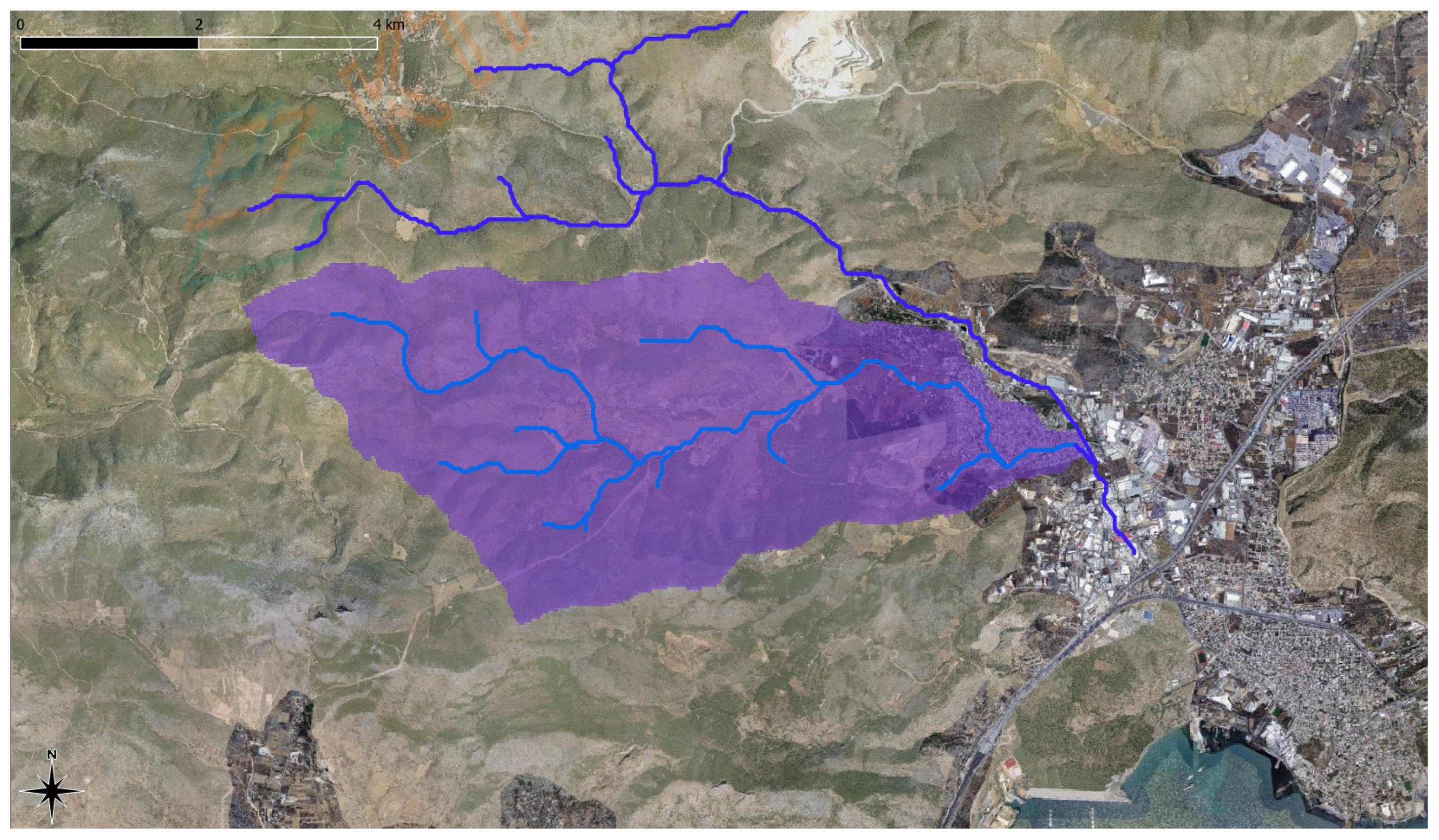
The city of Mandra is crossed by two creeks, Sures and Agia Aikaterini. The Agia Aikaterini flows directly through the urban fabric into an artificial underground culvert, while the Sures creek reaches the northern suburbs of the city, flows around the city and eventually contributes to the Agia Aikaterini stream at the eastern end of the city. The culvert channeling the Agia Aikaterini flow had a discharge capacity of 10 m/s [13] (recently increased to 50 m/s) and crosses the central and southern part of the city before finally reaching the eastern end, where it contributes to the Sures stream (Figure 2). There are no flow measurements available for either of the two streams.
This report focuses on the Agia Aikaterini creek because it is the one that caused the greatest destruction within the city of Mandra. Specifically, the watershed of this stream has an area of 20 km (Figure 2). The surface of the watershed exhibits high permeability due to the prevalence of karst formations [5].
The storm event under study that caused the Mandra flash flood occurred between 14 November 2017 23:00 UTC and 15 November 2017 12:00 UTC. It was a highly localized phenomenon with extreme spatial and temporal variability. The precipitation depth estimate came from the X-band mobile polarimetric weather radar (XPOL) of the National Observatory of Athens. Total rainfall on Mount Pateras, above Mandra, exceeded 153 mm during the main 6 h storm [14,15], with instantaneous rainfall intensities reaching values of up to 120–140 mm/h. The precipitation data (open access, see [13]) have a spatial resolution of 200 × 200 m and a temporal resolution of 2 min. By spatial integration of the radar data, the areal rainfall time series of the historical event over the watershed area of the Agia Aikaterini waterfall was derived.
Because discharge measurements were not available, hydraulic methods were used to estimate the discharge based on the post-event observed flow depth (flood event 15 November 2017). These proxy data for Agia Aikaterini were produced by Bellos et al. [13]. The proxy data generation involved two distinct phases. In the initial phase, Bellos et al. [13] utilized the physics-based FLOW-R2D model, employing a Monte Carlo technique, to derive an ensemble of 100 flood hydrographs. These hydrographs were derived by solving the 2D Shallow Water Equations. The outcomes of this analysis align closely with findings from other researchers. For instance, the median of the 100 maximum discharge values reached 157 m/s, while Diakakis et al. [16] reported a corresponding value of 140 m/s. In the subsequent phase, Bellos et al. [13] conducted a calibration process to determine the confidence interval of the hydrograph. This calibration was based on a dataset comprising 44 points where maximum water depths were measured in Mandra town (collected during post-event analysis in the field). To achieve this, the 2D mode of the HEC-RAS software was employed. Through this process, it was determined that the optimal confidence interval amounted to 40%.
The evapotranspiration value, although playing an insignificant role, was included for the sake of completeness in the hydrological cycle. It was held constant at 0.0019 mm/2 min, corresponding to the monthly evapotranspiration of November (41.4 mm), as calculated in a previous study by Koutsoyiannis and Xanthopoulos [17].
3. The Hydrological—Conceptual—Model
As mentioned in Section 1, the employed hybrid approach uses a combination of conceptual and physically based models, with the conceptual online model running twice per day on our server, while the physically based model runs only once for each of the pre-defined multiple hydrological scenarios.
Conceptual hydrological models are simplified representations of the water cycle and its interactions within a watershed. They abstract complex hydrological processes into discrete components, such as reservoirs and channels, using simplified equations to describe their behavior. These models are valuable for their efficiency in computation and ease of parameterization, making them useful for practical applications in data-scarce regions or for rapid assessments. However, their simplicity may lead to less accurate results compared to physically based models, as they do not consider spatial variations or detailed physics. For this reason, to ensure the most suitable model for a specific case study, it is essential to explore alternative options and thoroughly assess their performance. This rigorous evaluation process helps align the chosen conceptual model with available data and hydrological conditions, thereby enhancing prediction accuracy.
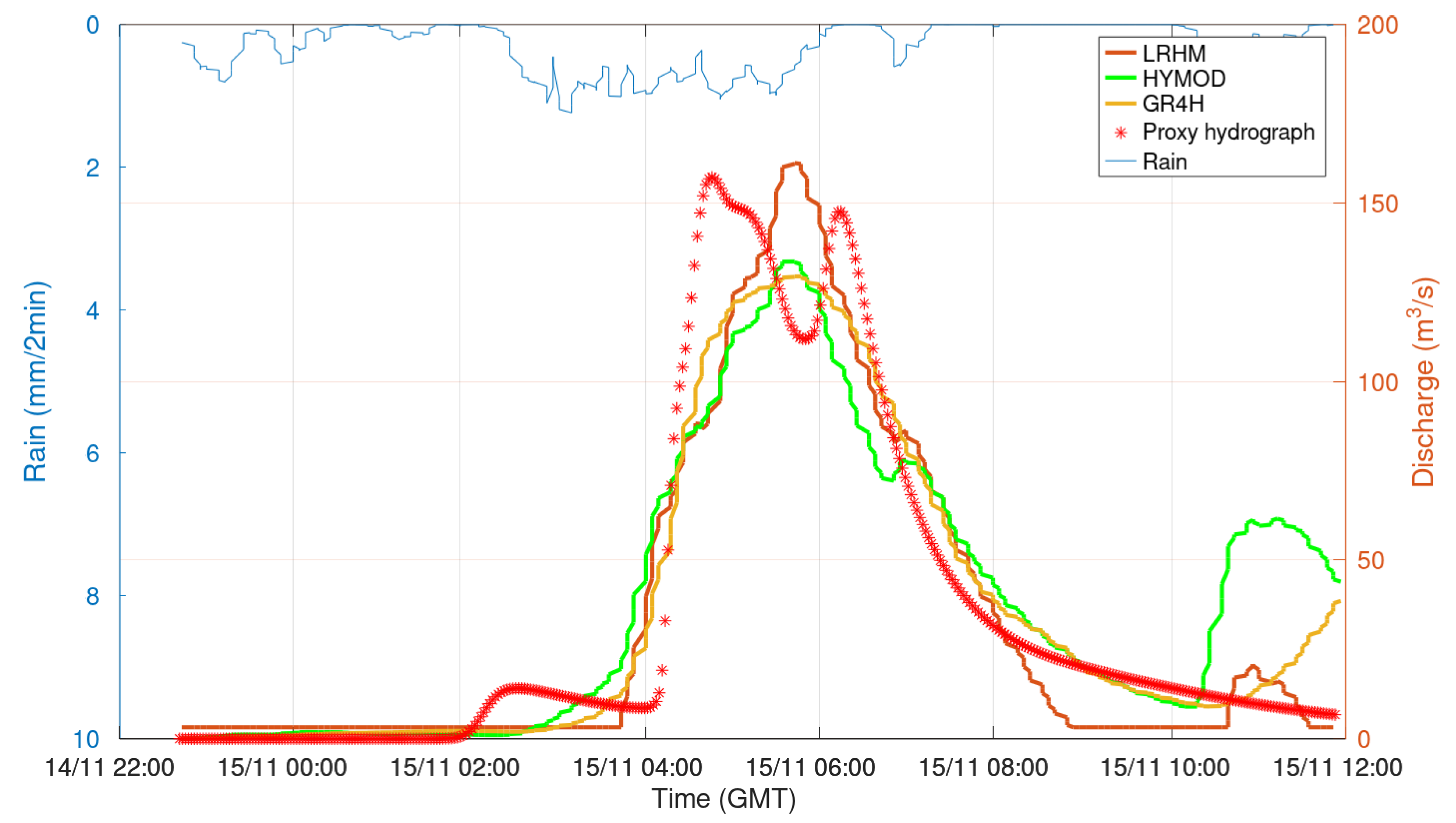
Guided by a recent study [18], we tested three hydrological models: HYMOD [19], GR4H [20], and LRHM [21]. Based on the findings from Rozos [18], GR4H exhibited the highest performance, boasting a lower number of parameters (five parameters for HYMOD, four parameters for GR4H, and six parameters for LRHM). Central to the investigation outlined in this manuscript, it is worth noting that all models underwent calibration utilizing the complete historical dataset. The calibration process was carried out using the Shuffled Complex Evolution (SCE-UA) algorithm, as detailed by Duan et al. [22,23]. The key objective function employed throughout this calibration was the mean squared error. The results for their simulations are displayed in Figure 3. GR4H achieved the best performance with a Nash–Sutcliffe efficiency (NSE) of 0.93. The NSE values of HYMOD and LRHM were 0.77 and 0.87, respectively.
An essential hydrological characteristic of the basin, influenced by its prevailing karstic terrain, is its negligible response to trivial precipitation events. Accurately simulating this behavior in the hydrologic model is of utmost importance. For this reason, a validation of the three hydrological models to a low-intensity hypothetical event was performed (this is actually the validation of the capacity of the models to reproduce the high infiltration rates expected in a karstic terrain). The hypothetical low-intensity rainfall was assumed to have a return period of 5 years whereas the hypothetical discharge was not expected to exceed the discharge capacity of the drainage network (before the capacity augmentation, i.e., 10 m/s). The reasoning is that this relatively frequent rainfall should not exceed the drainage network’s capacity; otherwise, Mandra would flood almost every second year. On the other hand, the return period was not set longer than 5 years because in Mandra, relatively frequent flooding phenomena occur [24,25]. For this reason, the ombrian curve (a.k.a. the intensity–duration–frequency curve) suggested by Markopoulos-Sarikas et al. [26] was used, which was constructed based on the data of the neighboring weather station of Eleusina (see Figure 1). Via this curve, the precipitation intensity for a return period of 5 years and a duration of 40 min was obtained, which was 39.2 mm/h. The 40 min period corresponded to the concentration time of the basin as it was estimated by a semi-empirical formula suggested by Efstratiadis et al. [27] for small-sized water basins. A uniform hypothetical rainfall of 40 min duration was considered. All three models offered maximum discharge values lower than 10 m/s (2.96, 3.76 and 3.22 m/s for GR4H, HYMOD and LRHM, respectively), which complies with the expected response from this watershed because of the high infiltration rates imposed by the hydraulic behaviour of the karstic terrain. Since all three models presented plausible simulations for the hypothetical low-intensity event, we opted for the model that achieved the lowest mean squared error for the application, which was GR4H.
4. The Physically Based—Offline—Model
The hydrological model can help to detect the exceedance of the discharge capacity of the flood control works, but it cannot estimate the impacts of an exceedance. For this purpose, a hydrodynamic simulation with a physically based model is required. Physically based hydrodynamic models are sophisticated numerical representations of real-world hydrological processes that simulate the complex interactions between water and its surroundings. These models use fundamental equations of fluid mechanics and other physics principles to simulate the flow of water in a catchment or river system. Unlike conceptual models, physically based models consider detailed spatial variations, such as the topography of the terrain and the hydraulic properties of different land surfaces. By accounting for intricate hydraulic structures and small-scale features, these models can offer valuable insights into flood behavior and potential impacts. However, their application may require significant computational resources and data input, making them more computationally demanding compared to conceptual models.
The increased computational burden poses a significant challenge for applications that require the generation of real-time inundation maps for decision-making. To address this issue in the present application, a solution inspired by the approach of Bhola et al. [28] was implemented. This involved constructing a database of high-resolution synthetic inundation maps using a 2D hydrodynamic model for a wide range of synthetic hydrographs. When an exceedance occurs, the appropriate inundation map is retrieved from the database. Evaluating this method, Bhola et al. [28] compared the retrieved inundation maps with those produced by a hydrodynamic model simulation. The results of the comparison were highly encouraging, revealing negligible deviation between the two maps.
While physically based models offer advanced capabilities for detailed flood simulations, their suitability should be carefully evaluated based on the specific characteristics and data availability of the study area. This evaluation process ensures that the chosen physically based model aligns effectively with the hydrological conditions of the target region. In this particular application, HEC-RAS was selected because it achieved the best combination of speed, simplicity, and accuracy. It is the same model that was used by Bellos et al. [13] to obtain the proxy observations (see Section 2). In fact, for this specific watershed, Bellos et al. found that HEC-RAS outperformed commercial programs, as the latter tended to overestimate flow depths despite considering the volumetric effects of urban structures (e.g., buildings). HEC-RAS was applied with a spatial resolution of 5 × 5 m whereas the time step was 1 s (input time series time step 2 min).
5. Synthetic Rainfalls and Inundation Maps
To construct the inundation map database, the initial step involved preparing a set of synthetic hydrographs. These hydrographs were then individually used as input for the HEC-RAS 6.4.1 software. Consequently, each synthetic hydrograph corresponds to an inundation map resulting from the HEC-RAS simulation, which is subsequently stored in the database. The more extensive the collection of synthetic hydrographs and their corresponding stored maps, the greater their representation of conditions during alarming events. For instance, Bhola et al. [28] stored 180 maps in their database (note that their study area was larger than the one studied here).
The synthetic hydrographs were generated using the conceptual hydrological model (GR4H) with input synthetic watershed areal rainfalls, which were generated using the Alternating Block method [29]. The Alternating Block was selected because according to a recent study that compared five methods used in developing design hyetographs, Alternating Block along with the Keifer and Chu model offered hyetographs closer to the observed [30]. Also, Koutsoyiannis’ work [31] showed that it leads to plausible hyetographs and hydrographs.
To apply this method, one must first define a time resolution , which in this case is equal to the time step of the hydrological model. Next, n blocks are formed, with representing the total duration of the synthetic rainfall. The rainfall depth of the ith block, where , is obtained using the following formula:
where idf is the ombrian curve, and T is the return period. From these n blocks, the hyetograph is assembled by placing the block with the highest rainfall intensity in the center of the duration of the synthetic event, followed by the remaining blocks, alternately, to the right and left of the center.
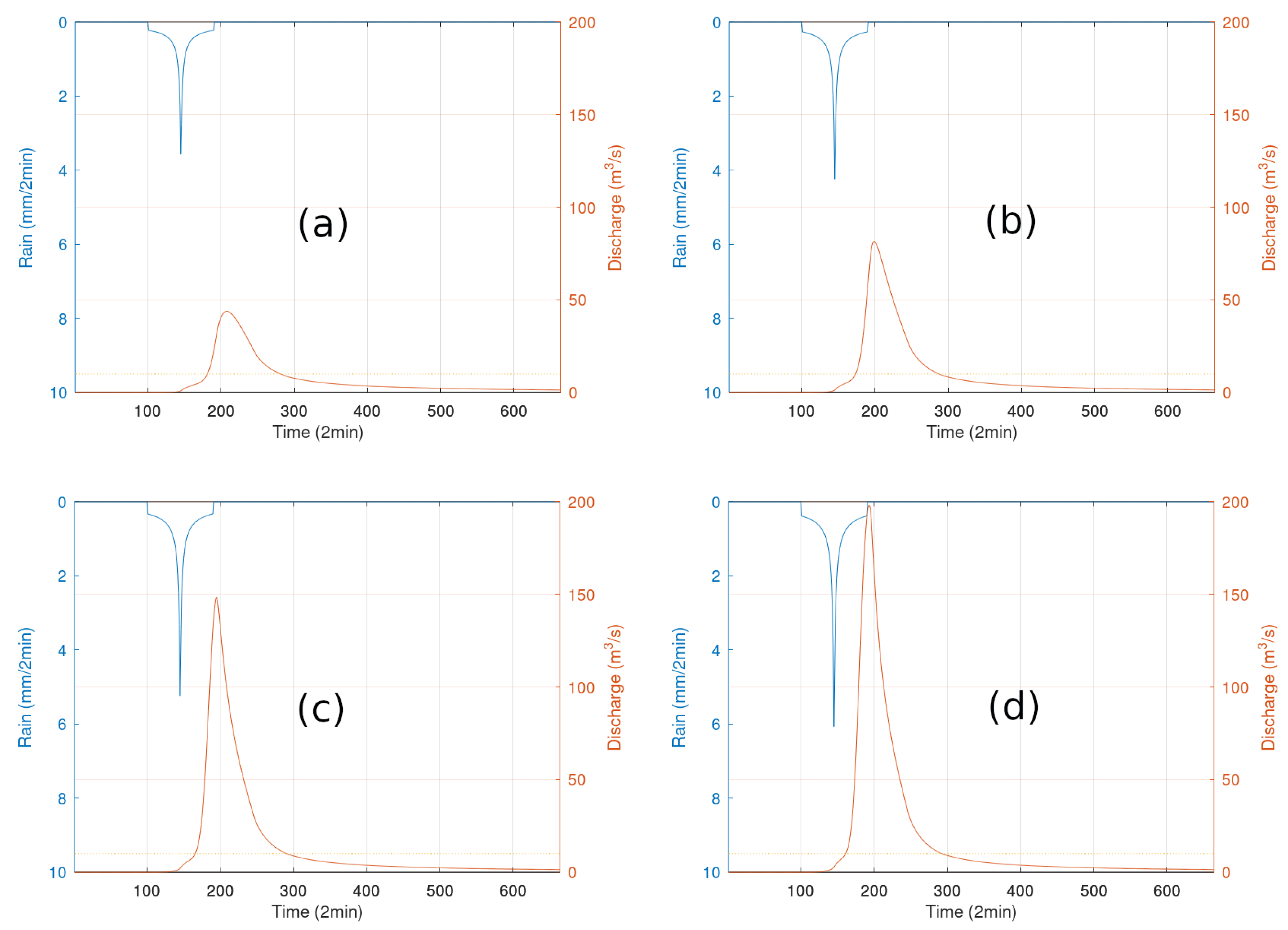
Figure 4 displays four synthetic hyetographs, produced with the Alternating Block method, and the corresponding hydrographs. The synthetic hyetographs have a duration of 3 h and a total depth of 50, 60, 74 and 85 mm. The hydrograph shown in panel (c) of Figure 4 closely resembles the hydrograph depicted in Figure 3 (representing the historical hydrograph reconstructed from proxy data).
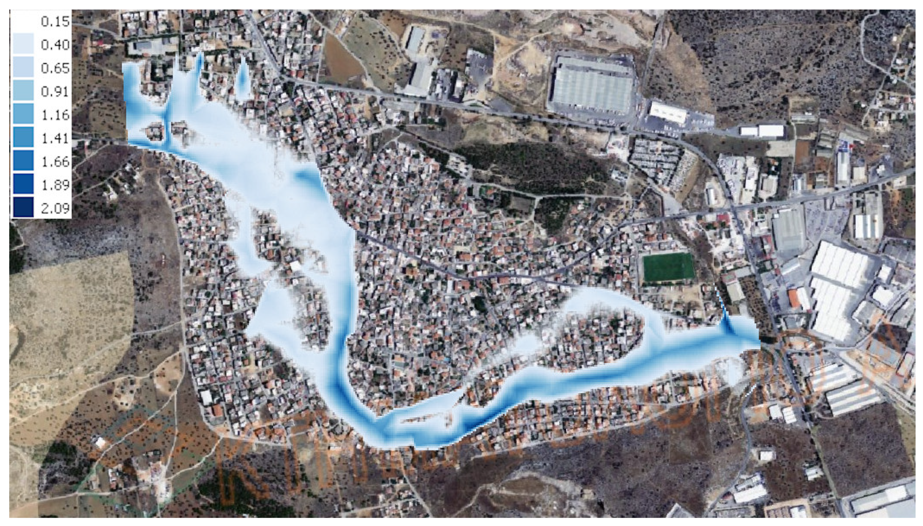
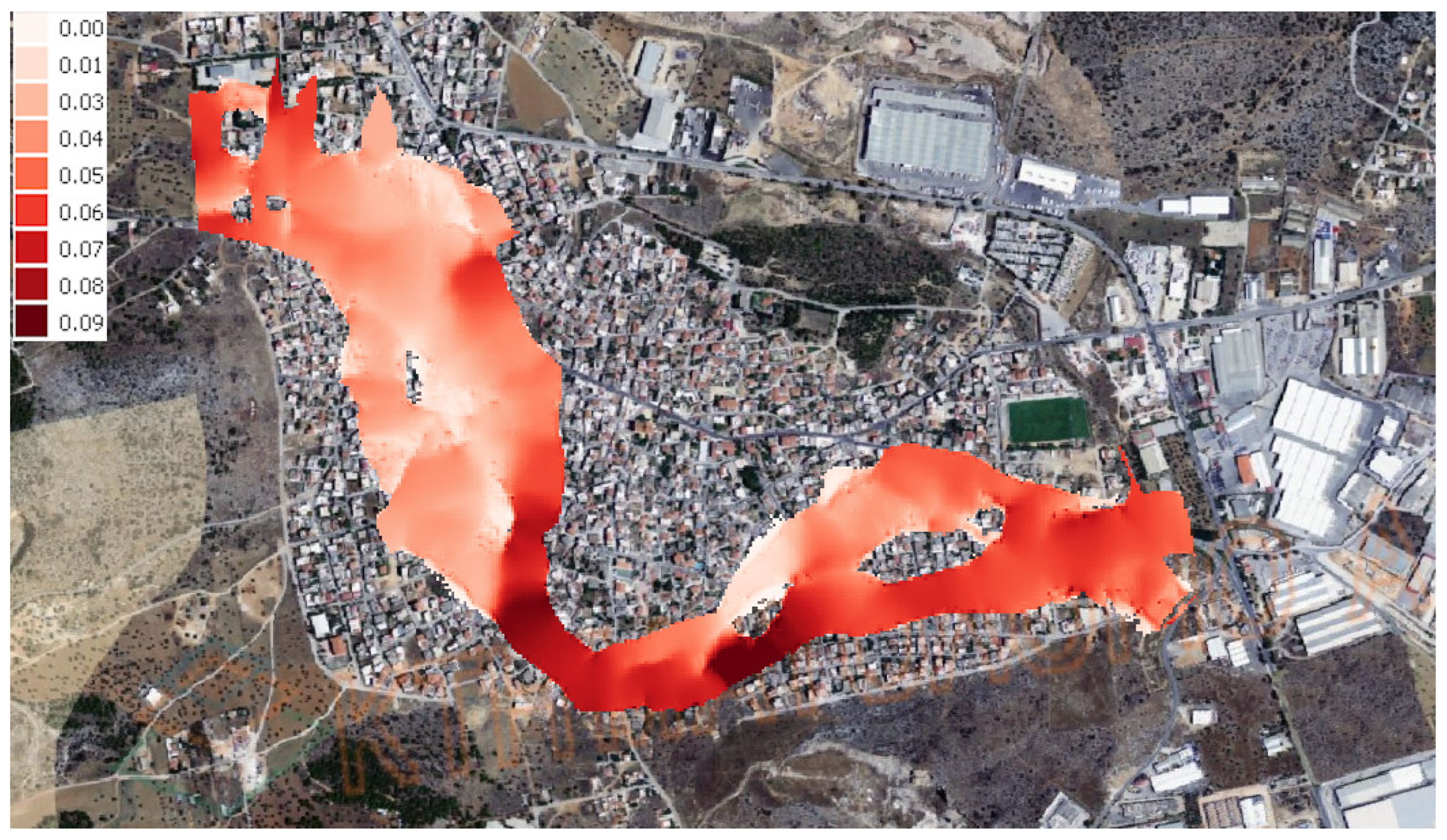
The synthetic hydrographs were utilized as inputs for the HEC-RAS model, enabling the pre-simulation of the potentially flooded areas. Figure 5 displays the map of flooded areas when using the observed (proxy) hydrograph, whereas Figure 6 presents the difference between the inundation map of Figure 5 and the inundation map obtained from the HEC-RAS simulation using the synthetic hydrograph from panel (c) of Figure 4. Figure 6 reveals that the inundation map based on the synthetic hydrograph is very close to that obtained from the historical proxy data.
The successful alignment between synthetic and observed hydrographs is crucial for establishing the credibility of using synthetic rainfalls as a valuable tool for assessing flood risk and preparedness. The minimal differences highlighted in Figure 6 suggest that synthetic hydrographs can accurately approximate historical hydrographs. Nevertheless, in applications of this nature, the crucial aspect pertains to the ability of synthetic rainfalls to generate plausible hydrographs that, in turn, yield inundation maps representative of those that might arise from an actual event. This aspect is further examined in the next section.
6. Disaggregation of Coarse Time Step Forecast Output
In early warning systems, rainfall time series are typically provided by forecast services. However, these forecasts often operate with larger time intervals than the time steps required by hydrological models. These finer time steps are essential for capturing detailed temporal nuances in hydrograph representation. To address this challenge, this study employs the Alternating Block method as a disaggregation tool.
The disaggregation with the Alternating Block method can be achieved employing the following steps:
- the return period T of each value of the forecast time series of the accumulated rainfall over the watershed is estimated from the ombrian curve, where the duration d is taken equal to the forecast time step ;
- synthetic rainfall time series with time step are produced with the Alternating Block—see Equation (1)—for the obtained T and from the previous step (the n is calculated by formula );
- the previous steps are repeated for all values of the forecast time series.
The effectiveness of this method is tested using the historical Mandra event of November 2017, evaluating its performance and applicability. In pursuit of this specific objective, the original 2 min areal rainfall time series for the watershed underwent temporal aggregation, transitioning into 3- h intervals. This time series is assumed to represent the forecast under operational conditions. By repeatedly applying the Alternating Block method to successive values of the 3 h time series, the aggregated time series was then disaggregated back to its original 2 min time step. The resulting 2 min time series was then used as input for the hydrological model. Ideally, the resulting hydrograph should closely approximate that obtained from the original 2 min areal rainfall time series.
Depicted in Figure 7, the sequence of 2 min rainfall time series is displayed, having been generated through consecutive applications of the Alternating Block method to the 3 h time series acquired subsequent to the aggregation of the historical 2 min time series. Within these applications, a time resolution of 2 min was employed. Furthermore, the duration of each Alternating Block application was set equal to 3 h, while the return period T for each application was chosen in a manner that ensured the total rainfall depth equaled the corresponding value of the 3 h time series.
Figure 7 shows a satisfactory resemblance between the hydrograph resulting from the time series obtained through Alternating Block disaggregation and the hydrograph derived from proxy data. This underscores the potential for processing a forecast at a coarse time step using a disaggregation technique such as the Alternating Block, yielding time series appropriate for hydrological simulations. It is important to acknowledge, however, that the application of this method may yield imprecise information regarding the precise timing of peak flow events. Nonetheless, a valuable estimation of their magnitudes can reasonably be anticipated within an acceptable level of confidence.
7. Early Warning System Setup
This section outlines the organization and integration of the previously described methods to establish the early warning system.
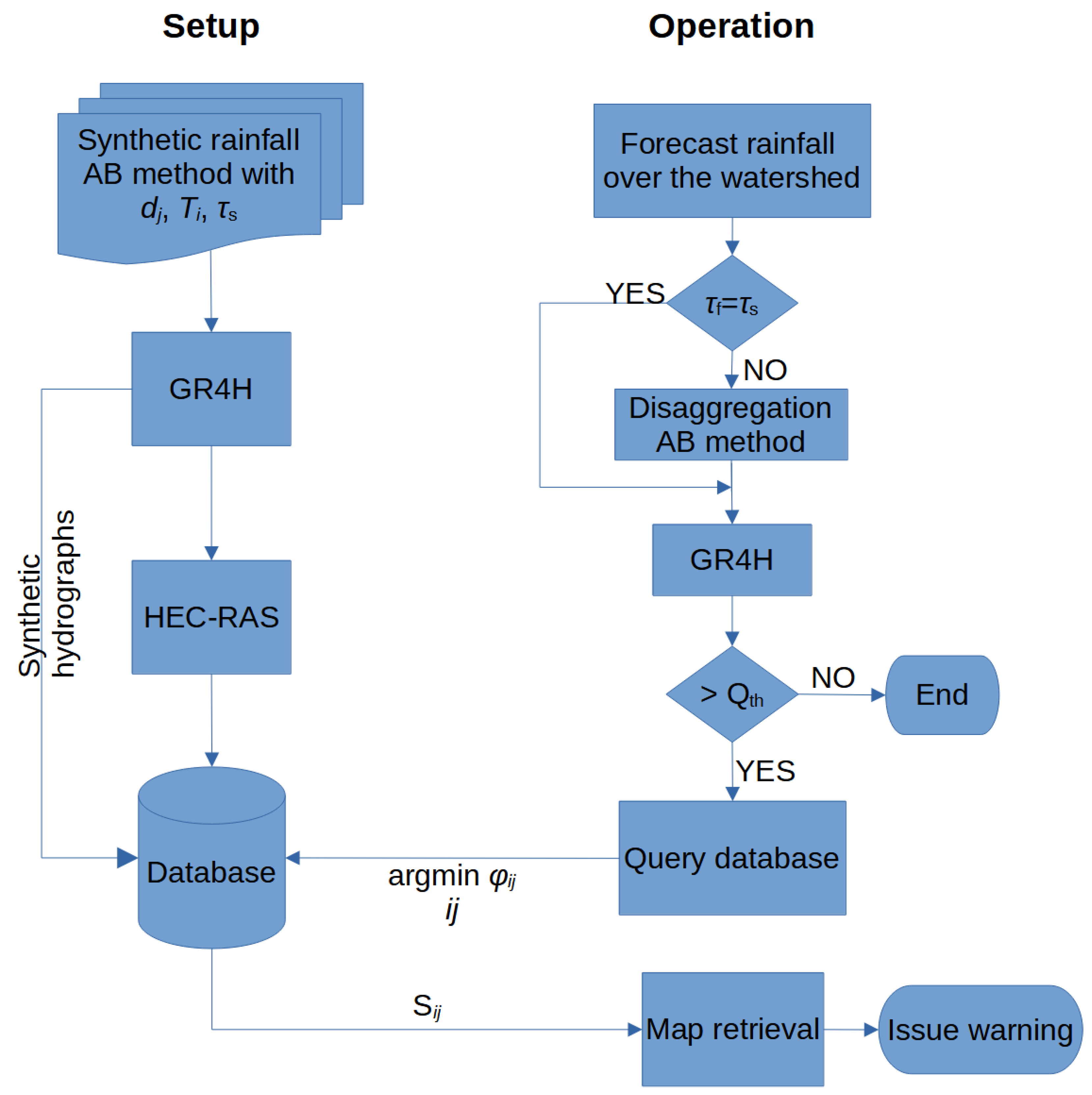
The operational phase includes obtaining the rainfall forecast and applying it as input to the GR4H hydrological model. If the hydrograph produced by the hydrological model does not exceed a warning threshold ( in Figure 8, essentially the discharge of the drainage network), then the procedure ends without sending a warning. If an exceedance occurs, the database is queried to retrieve the results of the hydrodynamic simulation that correspond to the closest stored synthetic hydrograph. Two issues that require consideration are how the forecast is made and how the database is queried.
Regarding the input time series of rainfall, one approach is to use rainfall data directly from weather radars. In this case, the time step of the forecast (or nowcast) rainfall time series can be set equal to the time step of the hydrological model . However, it is debatable whether this is the best possible approach since the fine temporal resolution increases the uncertainty, especially in small mountainous basins, where convective atmospheric conditions can be established rapidly leading to localized and intense storms (the case of the November 2017 Mandra event). It is advisable to use a larger time step for the rainfall time series () and then employ the Alternating Block method to disaggregate to the required time step ( in this case), as it provides an added safety margin in the modeling process.
Another approach can be to set up a local forecast service by extracting the boundary conditions from a global atmospheric circulation forecast model, and using them as initial or boundary conditions in a local area model, such as WRF-ARW [32]. This approach, without radar data assimilation, was applied as a pilot study in Mandra through the LOCOBUFLO project (additional information available at https://hydronoa.gr (accessed on 1 June 2023)). In that application, the forecast output time step was set at 3 h (the internal time step was much smaller), while the time step for the hydrological model was 2 min.
The rainfall time series obtained from the disaggregation with Alternating Block is utilized as input for the hydrological model, which operates with a time step . If the output of the hydrological model exceeds the warning threshold, then the most prominent curve of the hydrograph is isolated. This curve is compared against the synthetic hydrographs (stored in the database) used to obtain the pre-simulated inundation maps, and the closest one is retrieved. The comparison is made according to the following formula:
where is the stored in the database synthetic hydrograph produced with return period and duration —see Table 1 and Figure 8—S is the isolated hydrograph curve (e.g., the hydrograph between 16 November 2:00 and 16 November 7:00 of Figure 7) adjusted to align its peak with the peak of the synthetic hydrograph, is the base time of the synthetic hydrograph. The lowest indicates the inundation map that should be retrieved.
8. Discussion
In the operational phase of any early warning system, it becomes crucial to consider the inherent uncertainty associated with the interconnected processes. In our case, the flood early warning system consists of a series of sequential stages, where the output of one model serves as the input to the next. This interconnected arrangement involves a weather forecast model providing input to a disaggregation model, which, in turn, feeds into a hydrological model. Each of these models introduces its own uncertainties, which can propagate and accumulate throughout the system. Addressing and quantifying these uncertainties are of paramount importance as they directly impact the reliability and effectiveness of the early warning system.
Uncertainty in this context can be defined as a confidence interval for a designated confidence level, representing a range of possible outcomes. This interval quantifies the level of uncertainty associated with the predictions or results obtained at each stage of the early warning system. The confidence level reflects the degree of certainty that the true value lies within the specified interval.
To systematically address uncertainty propagation in the series of models, we calculate the total uncertainty step by step as the output propagates from one model to the next. In this case, each stage’s individual uncertainty can be quantified as follows.
- Weather forecast model. The output of this model is the forecast rainfall and the uncertainty is given by . Regarding the weather forecast, the uncertainty is often estimated using ensemble simulations; therefore, is expected to be provided by the forecast service.
- Disaggregation model. The input of the disaggregation model, which is the output of the weather forecast model, is and the output is the rainfall disaggregated down to the simulation time step. Its uncertainty can be estimated from experience obtained from applications of this method in similar case studies. For instance, Na and Yoo [30] reported that the Alternating Block method yielded a standard deviation of for the standardized difference between the maximum hydrograph values observed and those obtained through the method. For a confidence level equal to 95%, the confidence interval width, assuming a normal distribution of the errors, is , and the confidence interval is (0.548 is the mean value of the standardized difference given in [30]).
- Hydrological model. The hydrological model takes the output, , from the disaggregation model as its input and produces Q as its output. To efficiently handle uncertainty at this stage, we utilize random variables to represent the true (observed) hydrograph values as and the simulated values as . The distribution function of for a given can be estimated using the method proposed by Rozos et al. [33]. By calculating the confidence interval width for a 95% confidence level, denoted as , as , we can assess the uncertainty associated with the hydrological model. Notably, obtaining a reliable estimation of the hydrological model’s uncertainty necessitates hydrometric time series data of sufficient length, capturing a wide range of watershed responses.
- Hydrodynamic model. Although hydrodynamic simulations are based on mechanistic simulators, they still suffer from uncertainty issues. First, they incorporate several grey-box parameters, such as friction coefficients [34], which should be calibrated. Second, uncertainty can also arise from the information pertaining to topography, encompassing aspects such as grid resolution and the representation of hydraulic structures or buildings. Third, a fundamental limitation of the equations emerges in capturing the non-linearity of flow, particularly when dealing with intricate phenomena like floods. Lastly, as the equations are solved numerically rather than analytically, inherent errors are always associated with any numerical approach. Nonetheless, indications suggest that the primary origin of uncertainty is not linked to the structure or parameters of the hydrodynamic model, but rather to the driving factor, the input flood hydrograph [35].
In ideal scenarios without additional uncertainty at each stage i, propagating uncertainty through the early warning system could be achieved using formula for each stage i [36], where represents the input and the output of the stage i, and . However, due to the presence of uncertainty at each stage, the derivative becomes a function of and rather than a constant value. As a result, analytical estimation of uncertainty propagation is not feasible, and numerical methods like Monte Carlo simulations are required. In this context, considering three stages and employing n representative cases at each stage would result in a total of simulations. Fortunately, due to the minimal computational burden of the proposed method and the advancement in modern computing capabilities, the entire procedure is now expected to be completed within a mere 2 s (with parallel computing), even for a relatively large number of simulations, for example, 1000 for .
When considering the time step of the forecast time series, the 3 h output of forecast, employed also in this case study, is for the accumulated rainfall. The internal time step of the weather forecast model can be a couple of seconds, depending on grid resolution. In the typical 24 h weather forecast, a 3 h output time may be used in large watersheds. However, for smaller water basins, more accurate predictions are required. Having a WRF-AWR 3 h or 6 h forecast using assimilation of local radar data reduces significantly the error from input rainfall. For this reason, a nowcasting procedure, where the forecast is only up to 3–6 h, with a 15 min forecast output, is more suitable. This approach allows for higher precision and better responsiveness to rapidly changing weather conditions in small water basins, ensuring improved hydrological modeling outcomes [37].
Finally, considering the empirical method utilized to temporally disaggregate the forecast to match the time step of the hydrological model, a slight shift is anticipated between the peaks of the simulated and actual hydrographs (e.g., see Figure 7). It should be noted that the intensity profile of rainfall significantly influences the characteristics of a water basin’s response. Therefore, the utilization of idealized temporal patterns, such as the symmetric one used in the Alternating Block method, introduces uncertainties related to the shape of the rainfall profile. For example, Dunkerley [38], who compiled a dataset of four characteristic events from Fowlers Gap Arid Zone Research Station in western New South Wales, Australia, found that the time of occurrence of the peak flow heavily influences the peak discharge value, with late occurrences having a more adverse impact. Additionally, Barbero et al. [39] employed a shallow water hydrodynamic model to provide evidence of the variability of the lag time in small basins. They found that the intensity profile influences not only the runoff volume but also the lag time. Wright et al. [40] coupled stochastic storm transposition (SST) with storm catalogs developed from a ten-year high-resolution radar rainfall dataset for the region surrounding Charlotte, North Carolina, USA, to establish a more reliable method for obtaining design storms for flood risk assessment. They discovered that as storm duration increases, SST predicts that rainfall is more broadly distributed in time than that of the Alternating Block. Furthermore, they observed that at time scales longer than 1 h, 100-year rainfall tends to be multimodal. Interestingly, for the 1 h scale, which is the focus of this study, the Alternating Block method appears to provide a good approximation to the median values obtained by SST (see Figure 9 in [40]).
We would like to conclude by briefly discussing a recent devastating flood that occurred in Greece between 5 and 7 September 2023. During this event, we closely monitored the evolving weather conditions in the Attica region, with a particular focus on the Mandra water basin. We relied on three different forecasting services, including two national services and one international service, to provide inputs for our hydrological model. One of the national services predicted light rainfall across Attica but failed to anticipate two brief and intense precipitation bursts over the center of Athens. You can find online videos labeled “People are being swept away by powerful currents that occurred in the heart of Athens” documenting these events. The other two services predicted significant events over the Mandra basin, which did not materialize. Our monitoring of this event using the National Observatory of Athens radar (https://nowcast.meteo.noa.gr/en/radar/ (accessed on 5 September 2023)) revealed the prevalence of unsteady meteorological conditions with unpredictable establishment and subsequent dissipation of intense rainfall over relatively small areas (less than 50 km) within the broader Greek region affected by this meteorological event (approximately 90,000 km).
This event highlighted the challenges of implementing an early warning system for small water basins. An effective early warning system should minimize both false positive and false negative signals, primarily relying on the accuracy of weather forecasts. In the absence of ensemble simulations, one way to gauge this accuracy is by comparing forecasts issued at two or more consecutive times, as demonstrated in the LOCOBUFLO project at https://hydronoa.gr, (accessed on 1 June 2023). The closer the most updated forecast is to the previous one, the higher its reliability. However, this approach may not prevent false negative signals, as convective conditions in small hilly water basins can lead to unpredictable storms. This limitation is inherent in forecasts based exclusively on local area models. Consequently, radar-based short-term forecasts become essential in such applications. Additionally, the installation of sensors and on-site instrumentation plays a critical role in enhancing the system’s reliability (see bullet 3 in the discussion above) and extending valuable insights to other areas with similar conditions. These sensors and instrumentation not only improve the system’s effectiveness, but also facilitate rigorous performance testing and future enhancements.
9. Conclusions
This manuscript presents an efficient flood early warning system tailored for small-sized water basins with scarcity of hydrometric data and unique geomorphological characteristics, such as mountainous and karstic terrain, which contribute to localized and intense storm events. The lack of hydrometric data necessitated an improvised use of qualitative information collected after a catastrophic flood event to calibrate the hydrological model effectively.
To address the need for rapid response times and computational efficiency in this data-scarce environment, a database of pre-simulated, with a hydrodynamic model, flooding events was established. These simulations correspond to synthetic precipitations produced with the Alternating Block method. In operational conditions, the forecast precipitation is disaggregated using the same Alternating Block method, and the hydrological model is applied to assess the severity of the forthcoming event. By utilizing the pre-simulated events and the hydrological model, the system efficiently estimates potential flood events, aiding in real-time decision-making processes.
The flood early warning system developed, utilizing a hybrid combination of online/conceptual and offline/physically based modeling approaches, offers a promising solution to effectively mitigate the impacts of flash floods, particularly in urban areas situated in small watersheds. The successful implementation of this system in Mandra demonstrates its adaptability and potential for application in other regions facing similar hydrological challenges. By establishing such systems, communities can significantly enhance their flood management strategies and bolster resilience, ultimately reducing risks and minimizing potential losses of life and property.
In the context of an early warning system, time is crucial for effectively alerting the population to potential hazards. The system developed in this study operates swiftly, providing alerts within seconds based on short-term rainfall forecasts (with a practical maximum lead time of two hours). However, it is essential to recognize the intricate relationship between the response time of the water basin (which remains short in small basins regardless of the lag time), the modeling chain’s performance, and the time required for decision making and alerting. To minimize decision time at the competent authority level, streamlining communication channels and employing predefined contingency plans are crucial steps in ensuring a rapid and effective response to emergencies, especially flash floods.
Author Contributions
Conceptualization, E.R.; methodology, E.R.; software, E.R. and V.B.; validation, V.B., J.K. and K.M.; formal analysis, E.R.; investigation, E.R., J.K. and K.M.; resources, E.R.; data curation, E.R. and V.B.; writing—original draft preparation, E.R.; writing—review and editing, V.B., J.K. and K.M.; visualization, E.R. and V.B.; supervision, E.R.; All authors have read and agreed to the published version of the manuscript.
Funding
This research received no external funding.
Data Availability Statement
The data used in this study can be found in [10].
Conflicts of Interest
The authors declare no conflict of interest.
Abbreviations
The following abbreviations are used in this manuscript:
| LRHM | Linear Regression Hydrological Modelling |
| HEC-RAS | Hydrologic Engineering Center River Analysis System |
| GR4H | Géenie Rural à 4 paramètres Horaire |
| HYMOD | Hydrological model |
| WRF-AWR | Weather Research and Forecasting—Advanced Research WRF |
References
- Petrucci, O.; Aceto, L.; Bianchi, C.; Bigot, V.; Brázdil, R.; Inbar, M.; Kahraman, A.; Kılıç, O.; Kotroni, V.; Llasat, M.C.; et al. EUFF (EUropean Flood Fatalities): A European flood fatalities database since 1980. Earth Syst. Sci. Data Discuss. 2020, 2020, 1–30. [Google Scholar] [CrossRef]
- Georgakakos, K.P.; Modrick, T.M.; Shamir, E.; Campbell, R.; Cheng, Z.; Jubach, R.; Sperfslage, J.A.; Spencer, C.R.; Banks, R. The flash flood guidance system implementation worldwide: A successful multidecadal research-to-operations effort. Bull. Am. Meteorol. Soc. 2022, 103, E665–E679. [Google Scholar] [CrossRef]
- Hofmann, J.; Schüttrumpf, H. Risk-Based Early Warning System for Pluvial Flash Floods: Approaches and Foundations. Geosciences 2019, 9, 127. [Google Scholar] [CrossRef]
- Georgakakos, K.P. On the Design of National, Real-Time Warning Systems with Capability for Site-Specific, Flash-Flood Forecasts. Bull. Am. Meteorol. Soc. 1986, 67, 1233–1239. [Google Scholar] [CrossRef]
- Ntigkakis, C.; Markopoulos-Sarikas, G.; Dimitriadis, P.; Iliopoulou, T.; Efstratiadis, A.; Koukouvinos, A.; Koussis, A.; Mazi, K.; Katsanos, D.; Koutsoyiannis, D. Hydrological investigation of the catastrophic flood event in Mandra, Western Attica. In Proceedings of the EGU General Assembly Conference Abstracts, Vienna, Austria, 4–13 April 2018; p. 17591. [Google Scholar]
- Mazi, K.; Koussis, A.D.; Lykoudis, S.; Psiloglou, B.E.; Vitantzakis, G.; Kappos, N.; Katsanos, D.; Rozos, E.; Koletsis, I.; Kopania, T. Establishing and Operating (Pilot Phase) a Telemetric Streamflow Monitoring Network in Greece. Hydrology 2023, 10, 19. [Google Scholar] [CrossRef]
- Li, Z.; Zhang, H.; Singh, V.P.; Yu, R.; Zhang, S. A Simple Early Warning System for Flash Floods in an Ungauged Catchment and Application in the Loess Plateau, China. Water 2019, 11, 426. [Google Scholar] [CrossRef]
- Tegos, A.; Ziogas, A.; Bellos, V.; Tzimas, A. Forensic Hydrology: A Complete Reconstruction of an Extreme Flood Event in Data-Scarce Area. Hydrology 2022, 9, 93. [Google Scholar] [CrossRef]
- Borga, M.; Comiti, F.; Ruin, I.; Marra, F. Forensic Analysis of Flash Flood Response. WIREs Water 2019, 6, e1338. [Google Scholar] [CrossRef]
- Bellos, V.; Papageorgaki, I.; Kourtis, I.; Vangelis, H.; Kalogiros, I.; Tsakiris, G. Reconstruction of a flash flood event using a 2D hydrodynamic model under spatial and temporal variability of storm. Nat. Hazards 2020, 101, 711–726. [Google Scholar] [CrossRef]
- Georgakakos, K.P. Analytical results for operational flash flood guidance. J. Hydrol. 2006, 317, 81–103. [Google Scholar] [CrossRef]
- Henonin, J.; Russo, B.; Mark, O.; Gourbesville, P. Real-Time Urban Flood Forecasting and Modelling—A State of the Art. J. Hydroinformatics 2013, 15, 717–736. [Google Scholar] [CrossRef]
- Bellos, V.; Kourtis, I.; Raptaki, E.; Handrinos, S.; Kalogiros, J.; Sibetheros, I.A.; Tsihrintzis, V.A. Identifying modelling issues through the use of an open real-world flood dataset. Hydrology 2022, 9, 194. [Google Scholar] [CrossRef]
- Diakakis, M.; Deligiannakis, G.; Andreadakis, E.; Katsetsiadou, K.N.; Spyrou, N.I.; Gogou, M.E. How different surrounding environments influence the characteristics of flash flood-mortality: The case of the 2017 extreme flood in Mandra, Greece. J. Flood Risk Manag. 2020, 13, e12613. [Google Scholar] [CrossRef]
- Spyrou, C.; Varlas, G.; Pappa, A.; Mentzafou, A.; Katsafados, P.; Papadopoulos, A.; Anagnostou, M.N.; Kalogiros, J. Implementation of a nowcasting hydrometeorological system for studying flash flood events: The Case of Mandra, Greece. Remote Sens. 2020, 12, 2784. [Google Scholar] [CrossRef]
- Diakakis, M.; Andreadakis, E.; Nikolopoulos, E.; Spyrou, N.; Gogou, M.; Deligiannakis, G.; Katsetsiadou, N.; Antoniadis, Z.; Melaki, M.; Georgakopoulos, A.; et al. An integrated approach of ground and aerial observations in flash flood disaster investigations. The case of the 2017 Mandra flash flood in Greece. Int. J. Disaster Risk Reduct. 2019, 33, 290–309. [Google Scholar] [CrossRef]
- Koutsoyiannis, D.; Xanthopoulos, T. Engineering Hydrology; National Technical University of Athens: Athens, Greece, 1999; p. 218. [Google Scholar]
- Rozos, E. Assessing Hydrological Simulations with Machine Learning and Statistical Models. Hydrology 2023, 10, 49. [Google Scholar] [CrossRef]
- Boyle, D. Multicriteria Calibration of Hydrological Models. Ph.D. Thesis, University of Arizona, Tucson, AZ, USA, 2000. [Google Scholar]
- Perrin, C.; Michel, C.; Andréassian, V. Improvement of a parsimonious model for streamflow simulation. J. Hydrol. 2003, 279, 275–289. [Google Scholar] [CrossRef]
- Rozos, E. A methodology for simple and fast streamflow modelling. Hydrol. Sci. J. 2020, 65, 1084–1095. [Google Scholar] [CrossRef]
- Duan, Q.; Gupta, V.K.; Sorooshian, S. Shuffled complex evolution approach for effective and efficient global minimization. J. Optim. Theory Appl. 1993, 76, 501–521. [Google Scholar] [CrossRef]
- Duan, Q. Shuffled Complex Evolution Method (SCE-UA). MATLAB CENTRAL. 2013. Available online: http://www.mathworks.com/matlabcentral/fileexchange/7671 (accessed on 20 January 2023).
- Mandra Attikis: Kathe Spiti Mia Istoria Katastrofis. 2023. Available online: https://www.kathimerini.gr/society/935301/mandra-attikis-kathe-spiti-mia-istoria-katastrofis/ (accessed on 20 January 2023).
- “Voyliakse” Ksana i Mandra: Plimmyrisan Spitia Kai Dromoi. 2023. Available online: https://www.lykavitos.gr/news/greece/vouliakse-ksana-i-mandra-plimmyrisan-spitia-kai-dromoi-videosphotos (accessed on 20 January 2023).
- Markopoulos-Sarikas, G.; Ntigkakis, C.; Dimitriadis, P.; Papadonikolaki, G.; Efstratiadis, A.; Stamou, A.; Koutsoyiannis, D. How probable was the flood inundation in Mandra? A preliminary urban flood inundation analysis. In Proceedings of the EGU General Assembly Conference Abstracts, Vienna, Austria, 4–13 April 2018; Volume 20. [Google Scholar]
- Efstratiadis, A.; Dimas, P.; Pouliasis, G.; Tsoukalas, I.; Kossieris, P.; Bellos, V.; Sakki, G.K.; Makropoulos, C.; Michas, S. Revisiting Flood Hazard Assessment Practices under a Hybrid Stochastic Simulation Framework. Water 2022, 14, 457. [Google Scholar] [CrossRef]
- Bhola, P.K.; Leandro, J.; Disse, M. Framework for offline flood inundation forecasts for two-dimensional hydrodynamic models. Geosciences 2018, 8, 346. [Google Scholar] [CrossRef]
- Chow, V.; Maidment, D.; Mays, L. Applied Hydrology; McGraw Hill: New York, NY, USA, 1988. [Google Scholar]
- Na, W.; Yoo, C. Evaluation of rainfall temporal distribution models with annual maximum rainfall events in Seoul, Korea. Water 2018, 10, 1468. [Google Scholar] [CrossRef]
- Koutsoyiannis, D. A stochastic disaggregation method for design storm and flood synthesis. J. Hydrol. 1994, 156, 193–225. [Google Scholar] [CrossRef]
- Wang, H.; Sun, J.; Zhang, X.; Huang, X.Y.; Auligné, T. Radar Data Assimilation with WRF 4D-Var. Part I: System Development and Preliminary Testing. Mon. Weather Rev. 2013, 141, 2224–2244. [Google Scholar] [CrossRef]
- Rozos, E.; Koutsoyiannis, D.; Montanari, A. KNN vs. Bluecat—Machine learning vs. classical statistics. Hydrology 2022, 9, 101. [Google Scholar] [CrossRef]
- Bellos, V.; Nalbantis, I.; Tsakiris, G. Friction Modeling of Flood Flow Simulations. J. Hydraul. Eng. 2018, 144, 04018073. [Google Scholar] [CrossRef]
- Bellos, V.; Tsihrintzis, V. Uncertainty aspects of 2D flood modelling in a benchmark case study. In Proceedings of the 17th Conference on Environmental Science and Technology (CEST2021), Athens, Greece, 1–4 September 2021; pp. 1–4. [Google Scholar]
- Taylor, J.R. An Introduction to Error Analysis: The Study of Uncertainties in Physical Measurements; University Science Books: Sausalito, CA, USA, 1997. [Google Scholar]
- Varlas, G.; Papadopoulos, A.; Papaioannou, G.; Dimitriou, E. Evaluating the Forecast Skill of a Hydrometeorological Modelling System in Greece. Atmosphere 2021, 12, 902. [Google Scholar] [CrossRef]
- Dunkerley, D. The importance of incorporating rain intensity profiles in rainfall simulation studies of infiltration, runoff production, soil erosion, and related landsurface processes. J. Hydrol. 2021, 603, 126834. [Google Scholar] [CrossRef]
- Barbero, G.; Costabile, P.; Costanzo, C.; Ferraro, D.; Petaccia, G. 2D hydrodynamic approach supporting evaluations of hydrological response in small watersheds: Implications for lag time estimation. J. Hydrol. 2022, 610, 127870. [Google Scholar] [CrossRef]
- Wright, D.B.; Smith, J.A.; Villarini, G.; Baeck, M.L. Estimating the frequency of extreme rainfall using weather radar and stochastic storm transposition. J. Hydrol. 2013, 488, 150–165. [Google Scholar] [CrossRef]
Figure 1.
Map showing the geographical surroundings of Mandra city. Background map from http://openstreetmaps.org/ (accessed on 26 July 2023). The inner and outer boxes give the geographical context for the following maps.
Figure 1.
Map showing the geographical surroundings of Mandra city. Background map from http://openstreetmaps.org/ (accessed on 26 July 2023). The inner and outer boxes give the geographical context for the following maps.

Figure 2.
Agia Aikaterini creek (light blue line) and its watershed (purple area), and Sures creek down (dark blue line) to their confluence. Background map from https://maps.gov.gr/gis/map/ (accessed on 5 June 2023). For the geographical context, see the outer box of Figure 1.
Figure 2.
Agia Aikaterini creek (light blue line) and its watershed (purple area), and Sures creek down (dark blue line) to their confluence. Background map from https://maps.gov.gr/gis/map/ (accessed on 5 June 2023). For the geographical context, see the outer box of Figure 1.

Figure 3.
Hydrograph of the historical event at the output of the Agia Aikaterini watershed, simulated with the three assessed hydrological models, and corresponding rainfall.
Figure 3.
Hydrograph of the historical event at the output of the Agia Aikaterini watershed, simulated with the three assessed hydrological models, and corresponding rainfall.

Figure 4.
Simulations of GR4H using synthetic rainfall produced with the Alternating Block method: (a) total rainfall depth 50 mm and maximum discharge 44 m/s, (b) 60 mm and 81 m/s, (c) 74 mm and 149 m/s, and (d) 85 mm and 198 m/s.
Figure 4.
Simulations of GR4H using synthetic rainfall produced with the Alternating Block method: (a) total rainfall depth 50 mm and maximum discharge 44 m/s, (b) 60 mm and 81 m/s, (c) 74 mm and 149 m/s, and (d) 85 mm and 198 m/s.

Figure 5.
Inundation map (maximum water depth in meters) simulated by Bellos et al. [13]. For the geographic context, see the inner box in Figure 1.

Figure 6.
Deviation in meters of the inundation map of Figure 5 from the inundation map produced by HEC-RAS with input the synthetic hydrograph displayed in Figure 4 panel (c). For the geographic context, see the inner box in Figure 1.

Figure 7.
Synthetic rainfall, produced with the Alternative Block method, equivalent to the historical, and corresponding hydrograph obtained by GR4H.
Figure 7.
Synthetic rainfall, produced with the Alternative Block method, equivalent to the historical, and corresponding hydrograph obtained by GR4H.

Figure 8.
Setup and operation of the early warning system. AB stands for “Alternating Block”.


Table 1.
Example of synthetic hydrographs stored in the database. A pre-simulated inundation map corresponds to each hydrograph.
Table 1.
Example of synthetic hydrographs stored in the database. A pre-simulated inundation map corresponds to each hydrograph.
| 15 min | 30 min | 1 h 30 min | |
|---|---|---|---|
| 5 years | S011 | S012 | S013 |
| 10 years | S021 | S022 | S023 |
| 25 years | S031 | S032 | S033 |
| 50 years | S041 | S042 | S043 |
| 100 years | S051 | S052 | S053 |
| 200 years | S061 | S062 | S063 |
| 250 years | S071 | S072 | S073 |
| 300 years | S081 | S082 | S083 |
| 400 years | S091 | S092 | S093 |
| 500 years | S101 | S102 | S103 |
Disclaimer/Publisher’s Note: The statements, opinions and data contained in all publications are solely those of the individual author(s) and contributor(s) and not of MDPI and/or the editor(s). MDPI and/or the editor(s) disclaim responsibility for any injury to people or property resulting from any ideas, methods, instructions or products referred to in the content. |
© 2023 by the authors. Licensee MDPI, Basel, Switzerland. This article is an open access article distributed under the terms and conditions of the Creative Commons Attribution (CC BY) license (https://creativecommons.org/licenses/by/4.0/).
Share and Cite
MDPI and ACS Style
Rozos, E.; Bellos, V.; Kalogiros, J.; Mazi, K. Efficient Flood Early Warning System for Data-Scarce, Karstic, Mountainous Environments: A Case Study. Hydrology 2023, 10, 203. https://doi.org/10.3390/hydrology10100203
AMA Style
Rozos E, Bellos V, Kalogiros J, Mazi K. Efficient Flood Early Warning System for Data-Scarce, Karstic, Mountainous Environments: A Case Study. Hydrology. 2023; 10(10):203. https://doi.org/10.3390/hydrology10100203
Chicago/Turabian StyleRozos, Evangelos, Vasilis Bellos, John Kalogiros, and Katerina Mazi. 2023. "Efficient Flood Early Warning System for Data-Scarce, Karstic, Mountainous Environments: A Case Study" Hydrology 10, no. 10: 203. https://doi.org/10.3390/hydrology10100203
Note that from the first issue of 2016, this journal uses article numbers instead of page numbers. See further details here.