
Numerical Modeling and a Parametric Study of Various Mass Flows Based on a Multi-Phase Computational Framework


Department of Civil and Environmental Engineering, University of Toledo, Toledo, OH 43606, USA
*
Author to whom correspondence should be addressed.
†
Present address: Department of Civil and Enviromental Engineering, Michigan State University, East Lansing, MI 48824, USA.
Geotechnics 2022, 2(3), 506-522; https://doi.org/10.3390/geotechnics2030025
Submission received: 20 May 2022
/
Revised: 10 June 2022
/
Accepted: 17 June 2022
/
Published: 22 June 2022
Abstract
:Gravity-driven mass flows are typically large-scale complex multi-phase phenomena involving multiple interacting phases. Various types of mass flows usually exhibit distinct behaviors in their formation, propagation and deposition. In such large-scale geological systems, many uncertainties may arise from the variations in material composition and phase behavior. The present study aims to investigate the important characteristics of some common types of mass flows including debris flows, mudflows and earth flows, based on a recently developed multi-phase computational framework, r.avaflow for flow simulation. Fractions of different phases are varied to reflect different characteristics of material composition of various mass flows and simulate the resulting flow behavior. The evolution of the critical entities during the flow motion, such as velocity, peak discharge, flow height, kinetic energy, run-out distance and deposition is examined; considerable differences among various flows are identified and discussed. Overall, the simulated mudflow cases develop higher velocity, peak discharge, kinetic energy, and longer run-out distance than the debris flow cases. The fluid fraction has a significant influence on the flow dynamics; a higher fluid fraction often leads to higher velocities and long run-out distances, but lower kinetic energy, and it also affects the final deposition and deposition pattern considerably. The present study shows promising potential of a quantitative approach to the physics and mechanics of mass flows that may assist in the risk assessment of such large-scale destructive geological hazards or disasters.
1. Introduction
Rapid gravity-driven mass flows continue to pose a significant threat to the society at large due to their destructive nature [1,2]. A mass flow event typically represents a large geological system that can contain debris, rock, mud, water, snow, ice, and potentially other materials entrained and carried along the path of the flow. For example, a recent landslide involving garbage with an estimated volume of 60,000 occurred at a Dona Juana landfill site in Bogota, Colombia. This translational sliding mass raises concerns whether the disposed waste led to creation of weak surface and sliding movement. Geological materials located on a downslope are susceptible to various mass movements, which have frequently led to loss of life and property, and extensive damage to public infrastructure [3,4,5,6]. It is vital to understand the mechanisms of mass flows in order to develop strategies for effective assessment and mitigation of their calamitous effects.
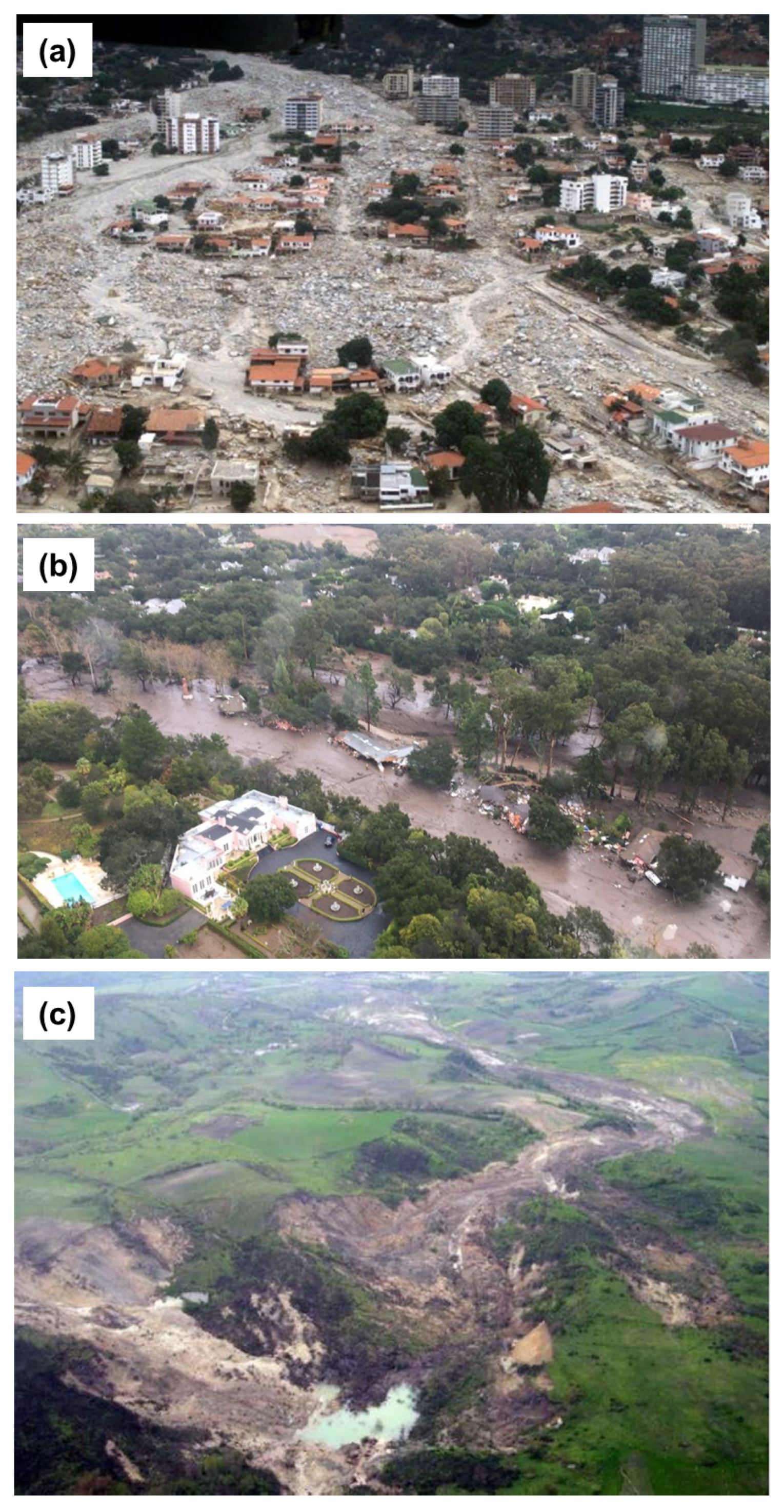
Several major forms of mass movements are defined in the well-known classification system that was proposed by Varnes [7] and later modified or refined by Hutchinson [8] and Hungr et al. [9], i.e., topple, fall, slide, spread, flow and complex. In each type of movement, the material type (e.g., rock, debris, earth) is a key factor in the further refinement of the specific type of mass movement. Of particular interest in the present study is the various flows that occur frequently around the world. Table 1 lists several prominent types of mass flows and their characteristics as summarized in Hungr et al. [9]. Figure 1 presents some photos of several cases of mass flow disasters. Figure 1a shows the debris flow destruction on the Caraballeda fan of the Quebrada San Julian in Venezuela in December 1999, which caused a death toll of over 10,000. Some of the debris flow deposits rose up to 6 m in height. The deposited large particles are clearly evident in the photo. According to Hungr [10], debris is defined as loose unsorted material of low plasticity that can be produced by mass wasting processes, weathering, glacier transport, explosive volcanism, or human activities. A debris flow typically contains a significant fraction of water whose presence facilitates the liquefaction of fine grains and renders the flow highly mobile; its velocity can become extremely rapid (e.g., over 10 m/s). Figure 1b shows the damage caused by a mudflow at Montecito, USA, resulting in at least 13 casualties. Mudflows typically involve predominantly clay-rich soil mixed with water at a high content, the large fraction of clay-sized soil particles may lead to even higher fluidity than debris flows. Figure 1c presents a photo of the Montaguto earth flow that took place in April 2006 in Southern Italy. Earth flows are often made up of fine-grained materials and the water content is usually much lower than in mudflows. Dry flow of granular material is often characterized as earth flow as well. Its velocity can range from extremely slow (e.g., m/s) to nearly rapid (e.g., m/s).
Risk assessment of large geological systems of mass flows can benefit from the improved understanding of the characteristics of different flow types, which, as discussed above, are considerably affected by the soil material composition and gradation and the water content. Although field monitoring and laboratory experiments can offer valuable information about the flow characteristics, such approaches usually come with certain limitations. For example, field observations and measurements only provide information after the event and the assessment of the relevant data collected from the field largely depends on reliable mathematical models to interpret the observed phenomena, while laboratory experiments are highly scaled down of actual field events, which may considerably alter the overall flow behavior. To quantitatively assess or predict mass flow characteristics in three-dimensional terrain, development of advanced dynamic mass flow models and relevant numerical simulations are often necessary and beneficial. In a quantitative approach to model the physics and mechanics of mass flows, the main challenge is the development of proper rheology to represent the distinctive behavior of various mass flows. Many models have been proposed based on single-phase framework, or a mixture approach, to describe the overall behavior of the material and model its evolution as a whole [11,12,13,14,15,16,17]; its rheology is at the core of the flow resistance, which may entail various possibilities such as frictional, Newtonian, Bingham, and turbulent or other fluid-like behavior. Such challenges are particularly difficult to overcome when one attempts to use a unified numerical model to simulate various types of mass flows, several efforts with the use of computational models such as Flo2D [18], RAMMS [19] and DAN3D [19,20] have been reported and shown promising potential.
A recently proposed multi-phase flow model by Pudasaini and Mergili [22] considers multiple phases in motion and incorporates many essential physical aspects of mass flows. It expands the theoretical formulations of a two-phase (solid and fluid) model of Pudasaini [23] with the introduction of a fine-solid phase; this allows more complex material behavior to be represented and considered in the modeling of the flow process. The first phase, the fluid phase is considered to a mixture of water and very fine particles such as silt, colloids, and clay; the latter are suspended in the water and their concentration may have an influence on the fluid yield strength [24,25]. The fluid rheology is considered to be shear rate dependent Herschel-Bulkley viscoplastic [26]. The second phase, termed as fine solid, contains fine gravel and sand. The rheology of this mixture is characterized by the rate-dependent visco-plastic behavior, as Jop et al. [27] show that dense granular flows shares similarities with classical visco-plastic fluids. In this model, shear and pressure-dependent Coulomb viscoplasticity is adopted for this fine solid phase; both viscous stress and yield stress can significantly affect the behavior of fine solid. The third phase, the solid phase is made up of boulders and coarser particles such as cobbles and gravels. Such coarse particles are generally considered as frictional materials with no viscous contribution. Thus Mohr-Coulomb plasticity is used for the solid phase. It is worth noting that this three-phase model has been shown to be capable of unifying several widely used models [13,15,23,28] by setting specific phase fractions.
The present study aims to better understand and compare the complex behavior of various types of gravity-driven mass flow by exploring the multi-phase model of Pudasaini and Mergili [22]. Fractions of different material phases are varied to represent different types of mass flow where each phase is characterized by its unique constitutive behavior. The present study focuses mainly on debris flows and mudflows, in addition to special cases of earth flows and complex flows as part of comparison. The various physical aspects of these flows are analyzed and compared to each other. Numerical simulation can be a great tool to understand the mechanics of mass flows and predict their behavior in time and space [29] and useful in establishing effective mitigation and remediation techniques, as the real-time field data is often scarce and the physical models of such large geotechnical systems are usually difficult to implement in laboratories.
2. Model Geometry and Various Flows Simulated
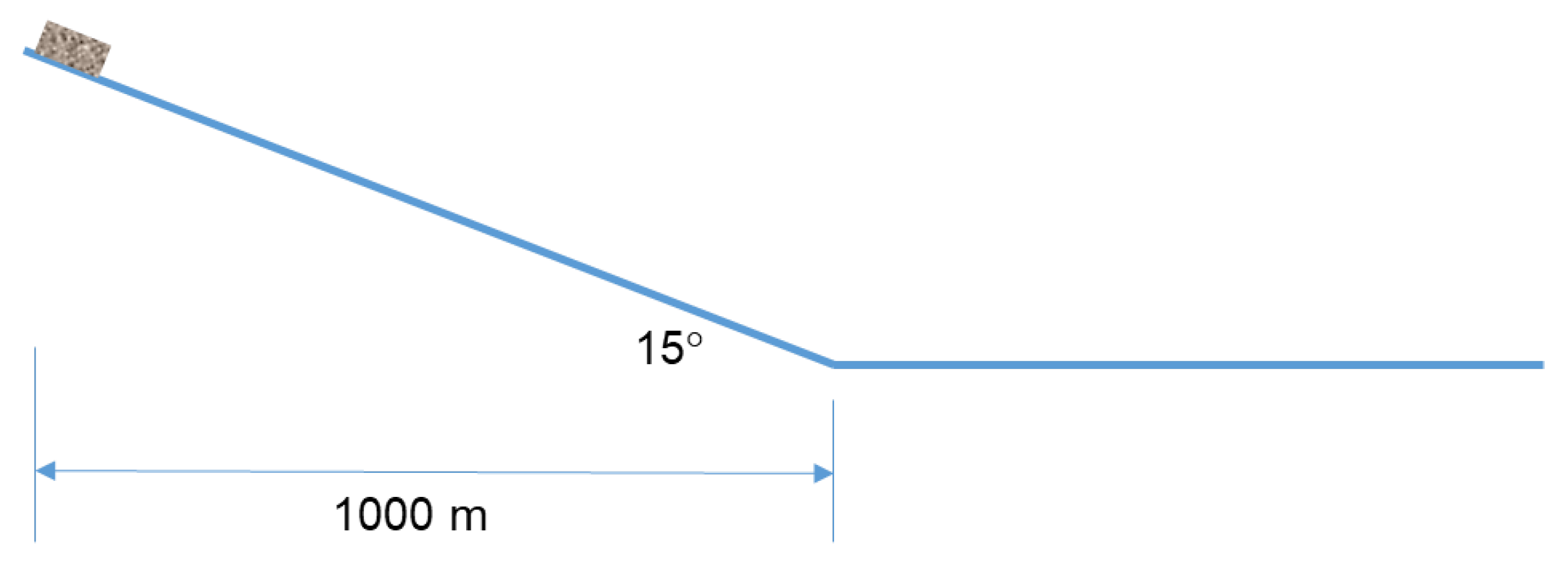
In the present study, various mass flows are investigated in the context of a large-scale geotechnical system where the gravity-driven motion of different types of large mass flow is simulated. The model is of a simple geometry of a slope of over a horizontal distance of 1000 m (Figure 2), and then the surface becomes flat along the horizontal direction where all traveling masses eventually deposit, resembling an alluvial fan in a geologic setting. The choice of this slope angle is based on the observation that it is a modest value within typical ranges of slopes in commonly observed geological disasters [30].
The two commonly occurring mass flows, namely, debris flows and mudflows, which are of considerable practical importance in geological hazard assessment, are the primary focus of the present study. In addition, two special types of flow, namely an earthflow with only fine solid phase, and a complex flow with an equal proportion of all three phases are also simulated for comparison purpose. This is achieved by varying phase fractions in the original mass as summarized in Table 2, which shows the notation used for various types of flows. The solid phase of debris flows is typically predominated by coarse particles and thus the simulated flows are assumed to consist of solid and fluid phases only. The fractions of each phase are also varied to produce five cases. Mudflows are assumed to contain fine solid phase and fluid phase because the solid fraction of mudflows is typically dominated by fine grains. An earth flow is studied by using only the fine solid phase to simulate a flow made of clay-rich fine-grained soil. A complex flow usually refers to a combination of two or more principal types of movement, as its behavior evolves from one type to another; in the present study a complex flow case is included by considering all three phases of equal fractions. It should be noted that varying the fractions of different phases to represent different mass flows is based on the general concept or observation of typical material compositions in the examined types of flows, in reality the formation of a specific type of flows in the field depends on a number of other factors, including the site’s geological history, geomorphological and topographic setting, environmental conditions and triggering events (e.g., rainfall, snowmelt, water level change, stream erosion, etc). In the present study the adopted parametric treatment reflects a simple approach to explore the intricacies of different flow behavior and one needs to be cautioned about its generalities and limitations in a proper perspective.
The initial mass is released in a block release scenario with a dimension of 50 m by 50 m. The total height of the initial release is 4 m. Hence the total volume of block release is 10,000 . The initial release height of the individual phases is varied based on the fraction of each phase depending on the flow type, and the volume of individual phases thus varies accordingly. The center point of block release is at 50 m from the left edge.
3. Numerical Implementation and Key Parameters
The software r.avaflow 2.0 [22] is used in the present study to simulate various flows. It is upgraded from its earlier version [31] to implement the above-mentioned three-phase model. It is a GIS supported open-source tool that can import actual topographic data for simulations. Obviously the present study revolves around a simple geometry and does not utilize this feature, however, field scale simulations of real world events using actual topographic data have been conducted and shown promising potential [32,33,34]. As a mass flow is generally comprised of multiple phases and the flow dynamics is strongly dependent upon the rheological properties of each phase, this three-phase model offers strong applicability for simulating various types of mass flows consisting of different material fractions. In addition, field observations of some past events and physical experiments also suggest that the three-phase mixture may be representative of the flow behavior [17,35,36,37].
The core part of the governing equations is established based on the universal equations of conservation of mass and conservation of linear momentum for each phase. The surface tension is assumed negligible and all three phases are considered incompressible and therefore possess a constant intrinsic density; no phase change is considered. It should be noted that the complex interactions among these phases are considered through the generalized interfacial forces, including the drag forces on the particulate phases, and the virtual mass force due to the relative acceleration between the phases. Depth-averaging is utilized to transform three-dimensional equations into two-dimensional equations, assuming that flows are long and wide compared to their depth. The details of the relevant mathematical formulations can be found in Pudasaini [23], and Pudasaini and Mergili [22].Table 3 summarizes the key material parameters for each phase in the present study. It is worth noting that the internal friction angle describes the internal frictional resistance of solid or fine-solid phase, whereas the basal friction angle characterizes the frictional resistance of the bed material on which the mass flow moves. The entrainment of material, which often occurs in debris flows, is not considered for the purpose of comparison among different flows. The results are generated with a time increment of one second for all the cases. The total simulation time varies depending upon flow characteristics.
4. Results and Discussion
A total of 12 cases summarized in Table 2 are considered in the present study; each different case is aimed to represent a distinct type of flow scenario in the field. The results obtained are used to examine the behavior of different mass flows. The physical parameters such as velocity, peak discharge, flow height, total run-out distance, final deposition height, deposition thickness and pattern, and kinetic energy are investigated.
4.1. Velocity and Peak Discharge
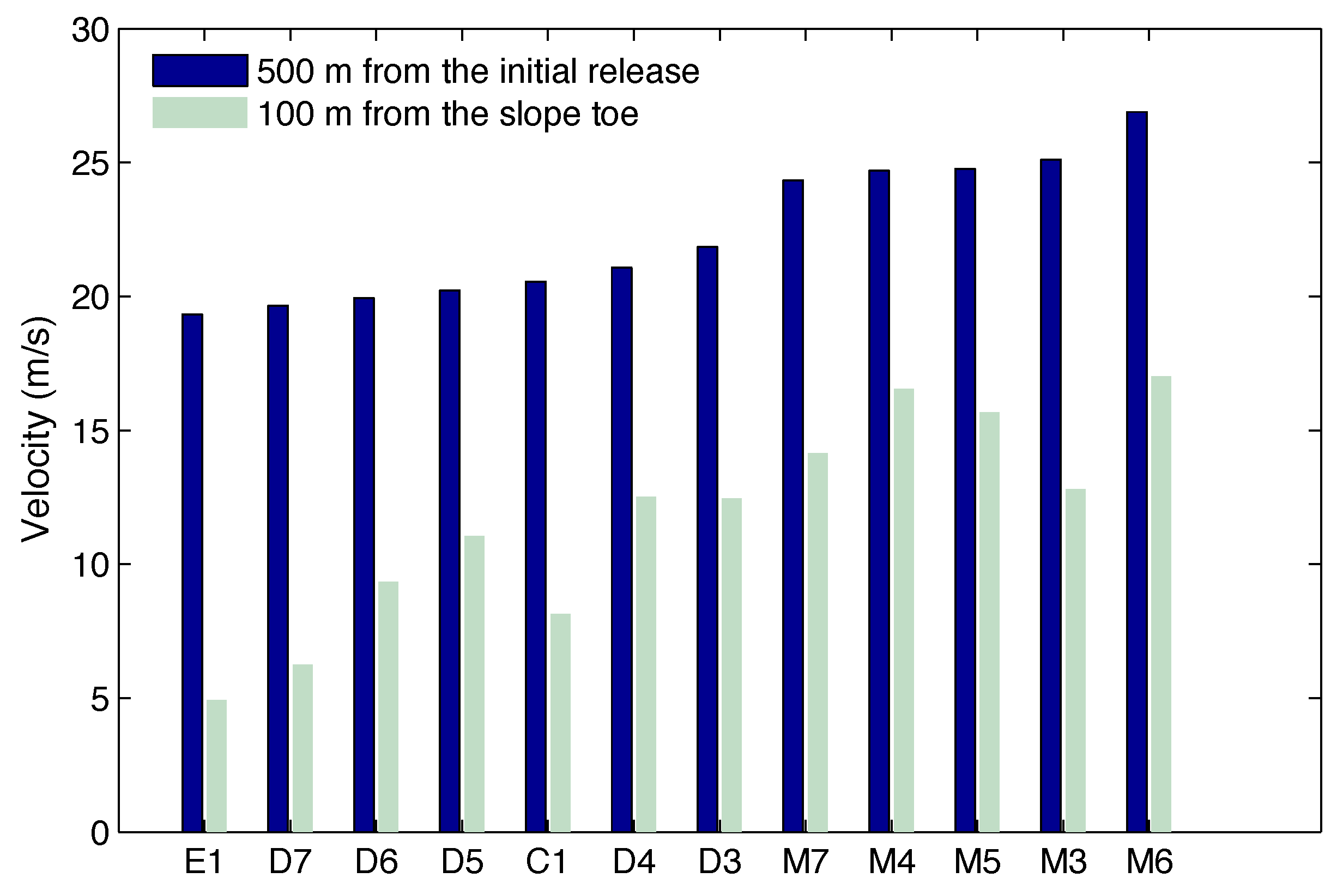
The velocities of flows along the centerline at two locations are selected for close examination and comparison: the first is around the mid-point of the slope, i.e., at a horizontal distance of 500 m from the initial release; the second is at 100 m away from the toe of the slope where the flow velocity is in decline after passing the slope and reaching the floor, but still maintains a reasonable high level. The results are summarized in Figure 3, which shows the velocities of all cases at 500 m from the initial release in ascending order, and accordingly their velocities at 100 m from the slope toe.
It is observed that the velocities of the mudflow cases are consistently higher than the debris flow cases, while the lowest velocity is found in the earthflow case (E1). The velocity also tends to generally increase with the increase in the fluid fraction for the debris flow cases. The higher velocity of mudflows can be attributed to their low values of the bed friction angle compared to debris flows. For the earth flow case, due to the absence of the fraction of fluid phase, its mobility is significantly reduced, leading to the lowest velocity. After the flow travels 500 m from the initial release, the maximum velocity of 26.88 m/s is found in the M6 case, while the lowest velocity of 19.33 m/s is found in E1 case. The velocities are significantly reduced after reaching the floor and a maximum velocity of 17.01 m/s and a minimum velocity of 4.92 m/s are found in the M6 and E1 cases, respectively, at 100 m from the toe of the slope; evidently the slope angle change has a great influence on the mass flows. However, it is worth noting that these mass flows still move at considerable velocities after reaching the toe of the slope and thus carry substantial destructive momentum.
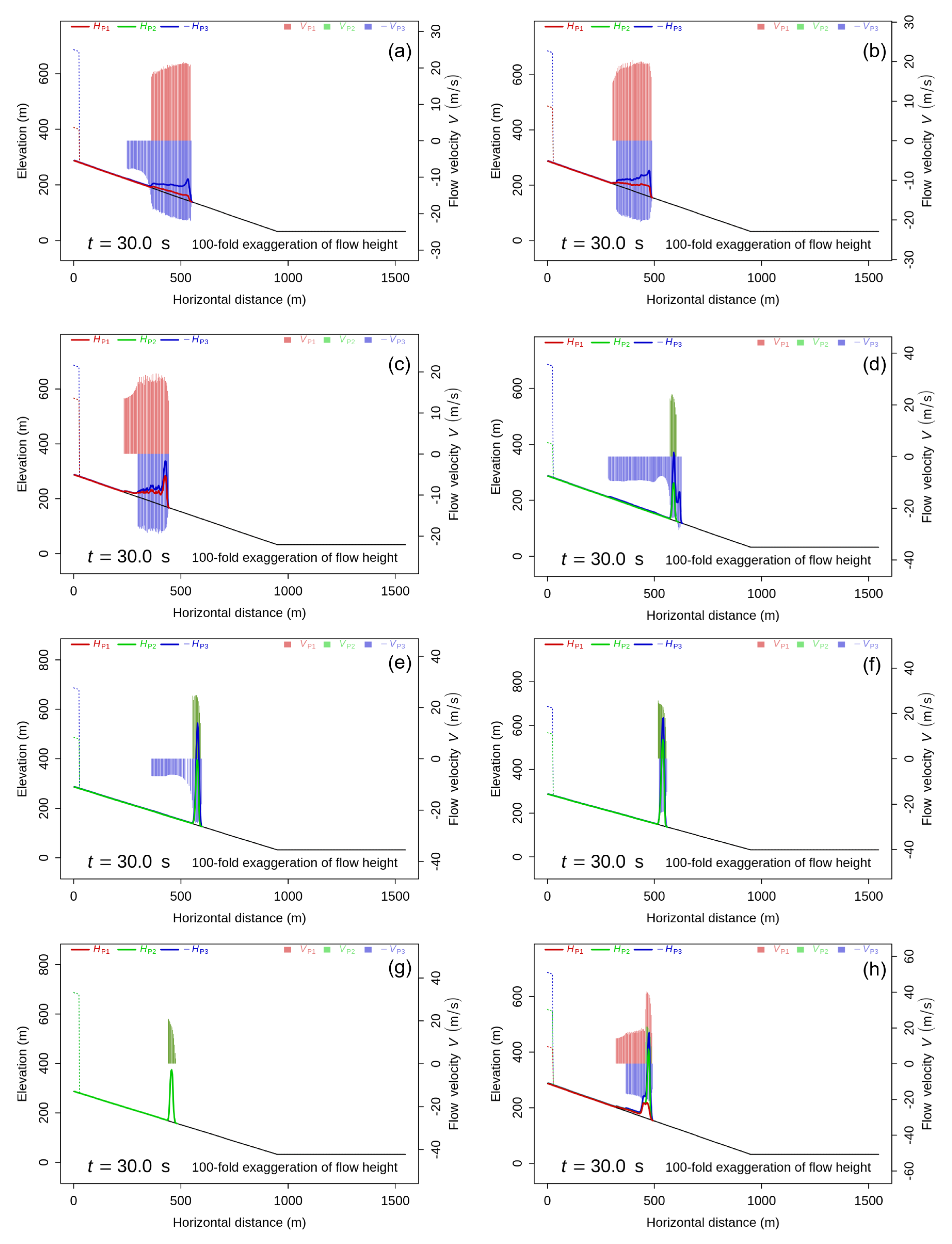
It is of interest to present the details of the flow velocity and height of individual phases for a few cases at a specific time moment, e.g., at 30 s after the flow initiation, as shown in Figure 4. This time instance is chosen because at this moment all flows approach or reach around a horizontal distance 500 m, half away from the initial release to the end of the slope; obviously the specific location varies in each case and it is of interest to examine the flow when it reaches the half away of the slope as discussed later. The velocity is represented by the bar chart, and the height by the solid line, which will be discussed in the next subsection. The results of the velocities are consistent with the trend in Figure 3. It also shows that the mudflows generally travel farther than the other cases after the same time duration. The higher velocities occur in the head (frontal part) of the flow compared to the tail. It also shows that for the mudflows and earth flow cases, the majority of fine solid is in the frontal part of the flow, while in the case of debris flow, the solid part is distributed along with the entire flow. This is possibly due to lower drag and virtual force applied on the fine solid particle compared to solid phase, because the drag force and the virtual mass force are lower when the density is lower and the surface area is smaller.
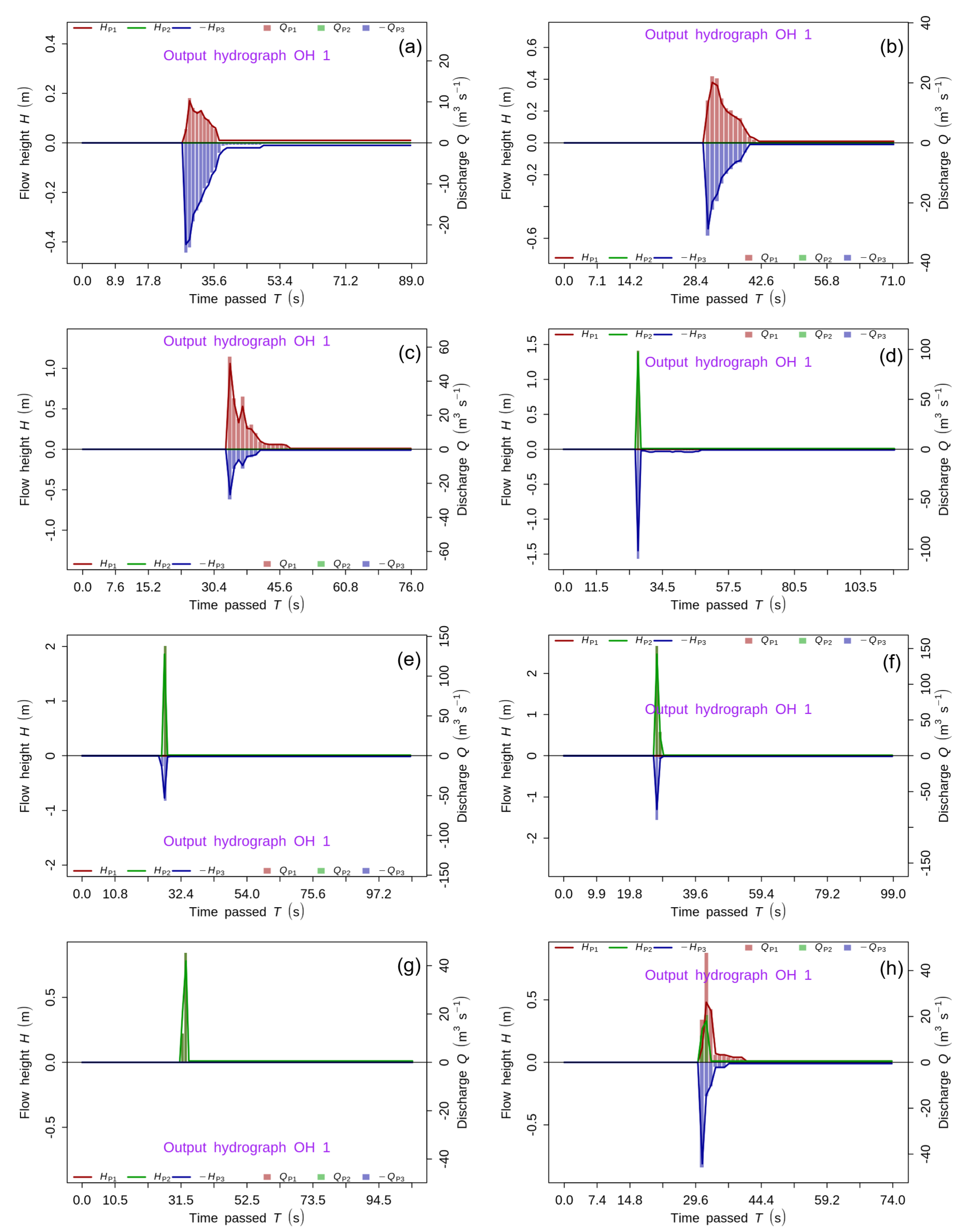
Similar to velocity, the discharge is also calculated at the same locations for different cases and presented in the hydrograph, which includes both the flow height and discharge passing through a specific location, as shown in Figure 5 and Figure 6. As expected, due to higher velocities, the magnitude of peak discharge for mudflow cases is very high compared to the debris flow cases. It is also evident that the effect of the solid/fluid ratio is significant on the magnitude of peak discharge, as shown by the results of the debris flow and mud flow cases. It is worth noting that all flows reach the mid-point of the slope around the time s, the earliest is in M3 case, which contains a large fluid fraction. At 500 m away from the initial release (Figure 5), the maximum peak discharge overall is observed in M7 case with a combined magnitude of 243.23 , which contains 153.54 of fine solid phase and 89.69 of fluid phases. The discharges of the earth flow and the complex flow are modest, between the debris flows and mudflows.
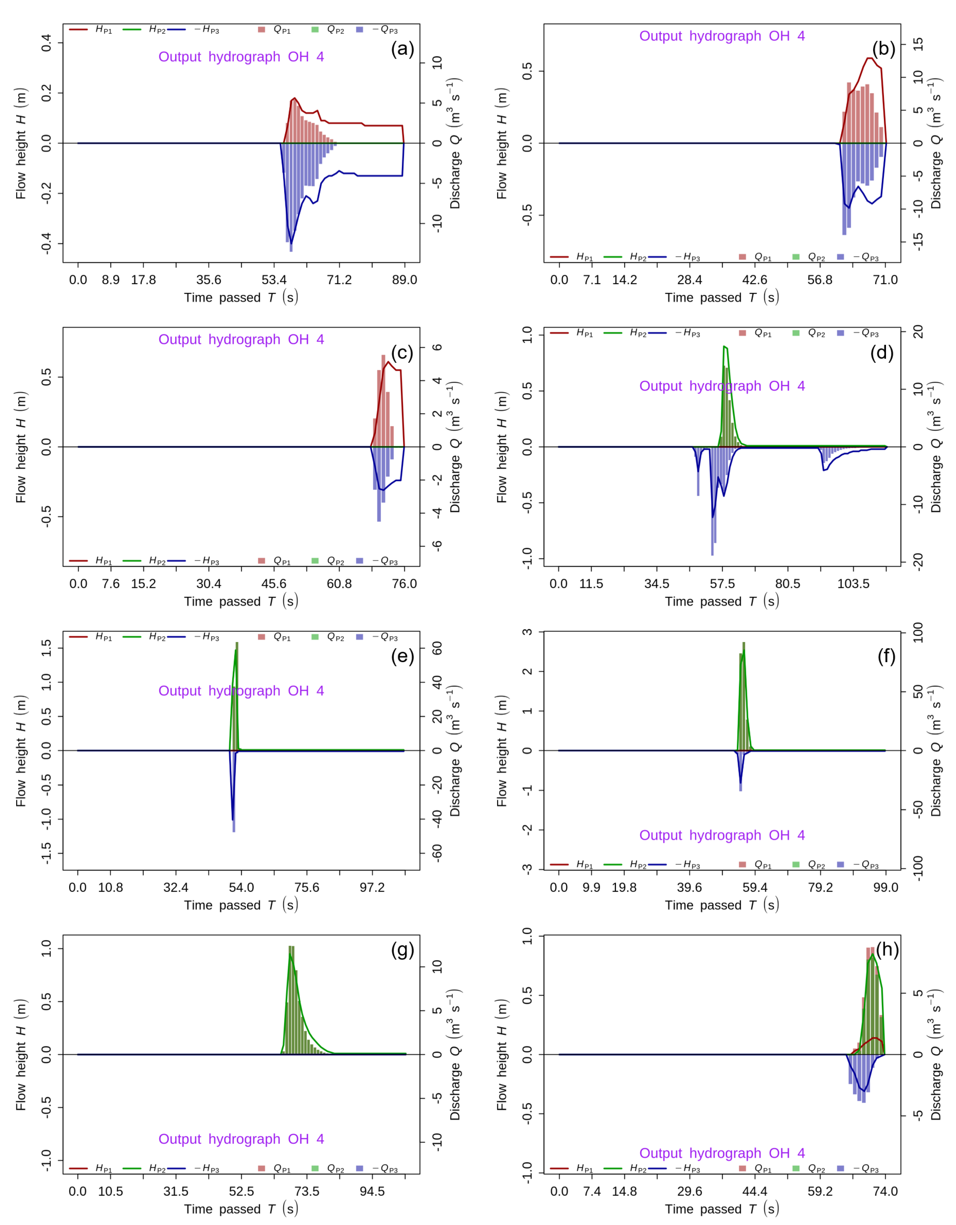
Discharge of each flow case at 100 m away from the toe of the flow (Figure 6) is significantly reduced after the flow reaches the horizontal part of the path. The time needed for each flow varies significantly, with M3 being the fastest ( s) and D7 the slowest ( s). Still the maximum peak discharge occurs in M7 case with a combined magnitude of 117.02 that contains 82.65 and 34.37 for fine solid and fluid phases, respectively. The decrease reflects the gradual deposition of material along its travel path.
4.2. Flow Height
Figure 4, Figure 5 and Figure 6 presented in Section 4.1 already include some results of the height of examined flows at a specific time or locations. Figure 4 shows the flow front of the debris flows is generally higher than the tail and the highest section is very close to the front, as commonly observed in many actual debris flow events in the field, although such a trend is not apparent in other types of flow. Overall the decline in the height of each phase in each flow with time is evidently notable, especially after it travels down the slope (Figure 5) and reaches the horizontal floor (Figure 6). The height of individual phases primarily depends on the initial volume or height of individual phase as the height of solid increases from D3 to D7 case.
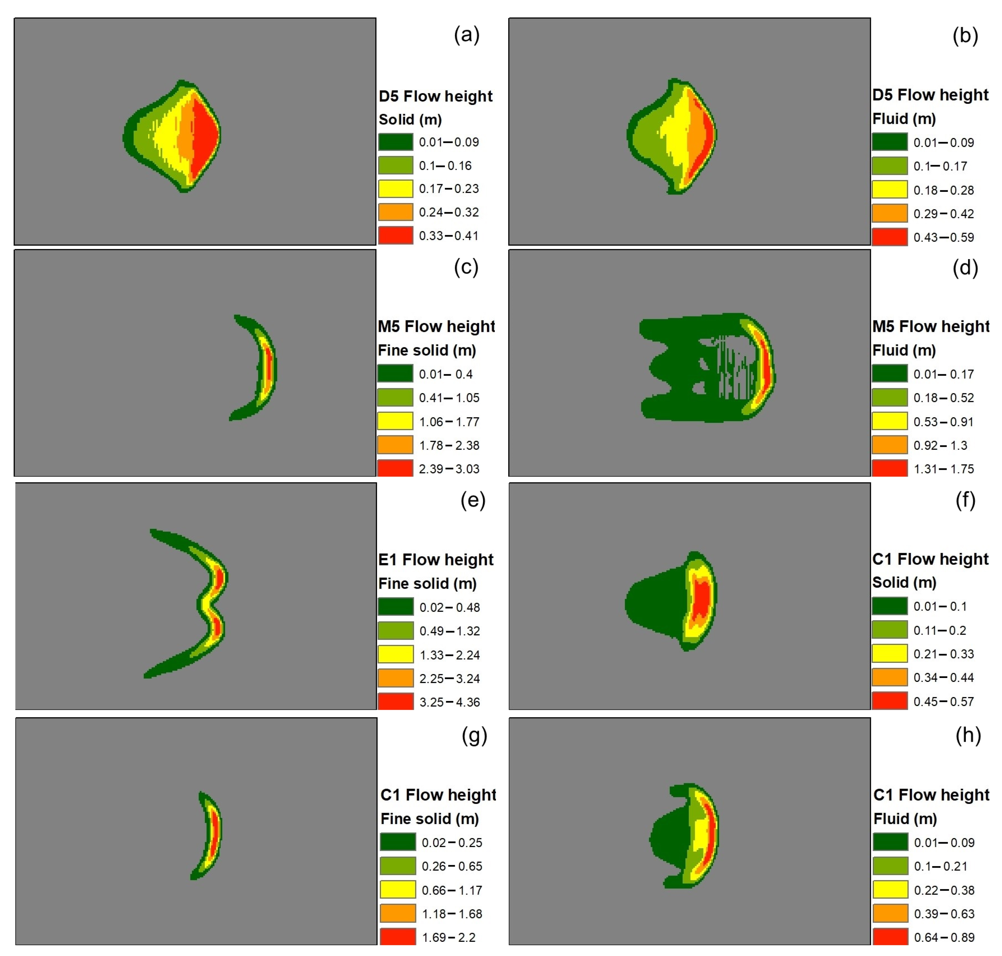
The height profiles of flow for individual phases for D5, M5, E1, and C1 cases at 30 and 50 s are presented in Figure 7 and Figure 8, respectively; for debris flows and mudflows, the cases with an equal proportion of phases are considered for comparison purpose. Figure 7a,b show that, for debris flow case D5, the formation of a lobe-shaped profile with the spreading of material laterally is evident. The contours of the height of solid and fluid phases are similar. The height of flow reduces from the frontal to the tail part. In the case of mudflow M5, there is no formation of the lobe, and no spreading of the material is observed for the fine solid case (Figure 7c). However, considerable spreading of flow occurs in the fluid phase and some fluid fraction clearly lags behind the front (Figure 7d). Due to the absence of longitudinal spreading, the height of the fine solid is significantly higher than the height of the fluid phase in the M5 case. The highest magnitude of 3.03 m is observed of fine solid phase in the front center of the flow. For the earth flow case, E1, the fingering phenomenon is observed due to significant lateral expansion of the fine solid material (Figure 7e). Similar to the mudflow case, the material does not spread longitudinally, and hence an increased height of 4.36 m is observed, showing that some soil material moves to join the front. In the case of complex flow, C1 with an equal proportion of the three phases (Figure 7f–h) the difference in the behavior of flow is clearly appreciable. The solid phase and fluid phase have significantly higher longitudinal and lateral spreading compared to fine solid case. Hence, the height of the fine solid phase is very high compared to other phases.
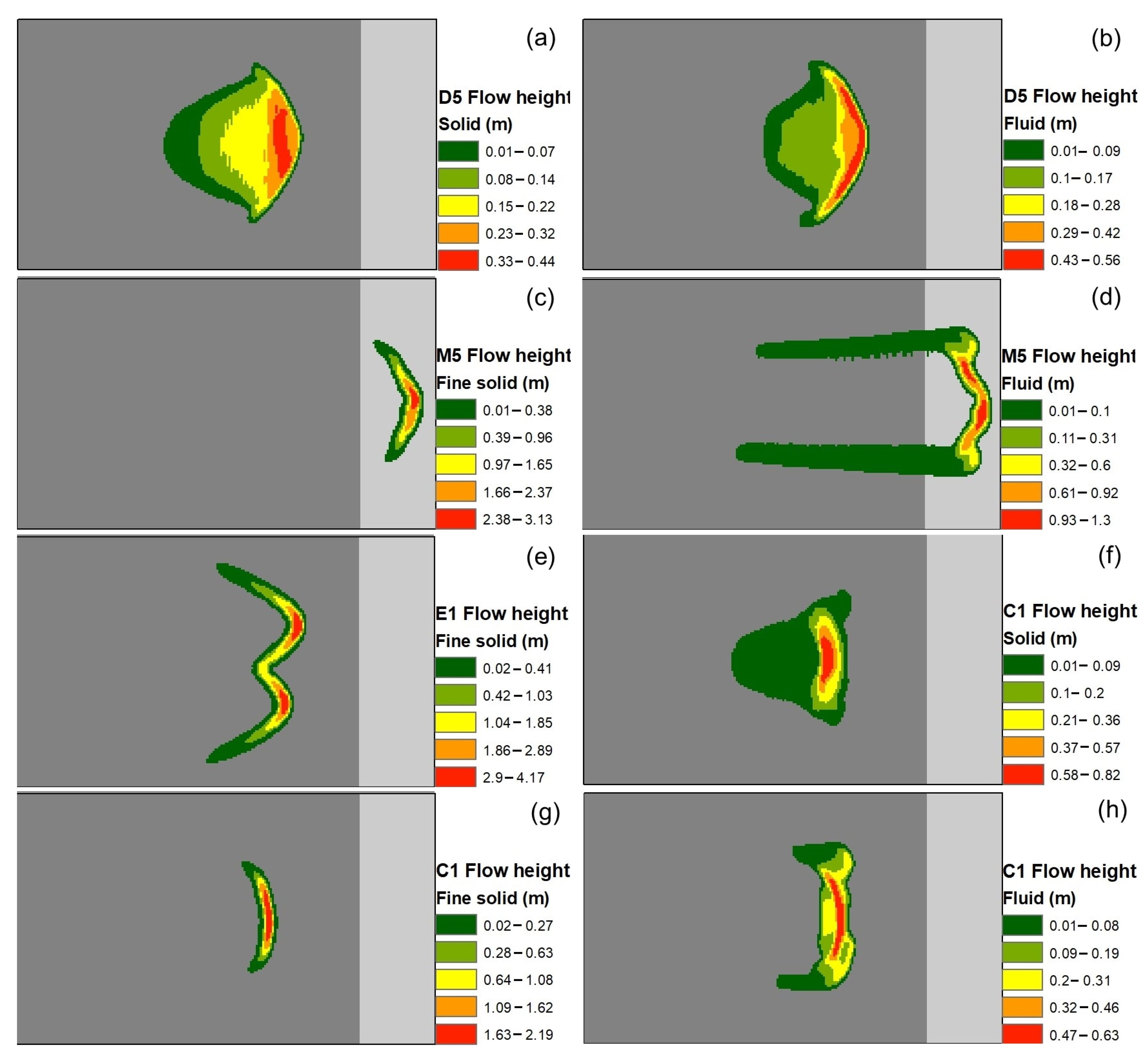
The above observations of flow characteristics are further manifested in Figure 8, which shows the simulation results at 50 s. Overall the lateral spreading expands to certain extent in each case compared to Figure 7. It is notable that the M5 flow already reaches the horizontal plane at this moment due to its high velocity as discussed earlier; its fingering effect is more remarkable in the fluids phase, indeed significant fractions of fluid are still on the slope and far behind the front.
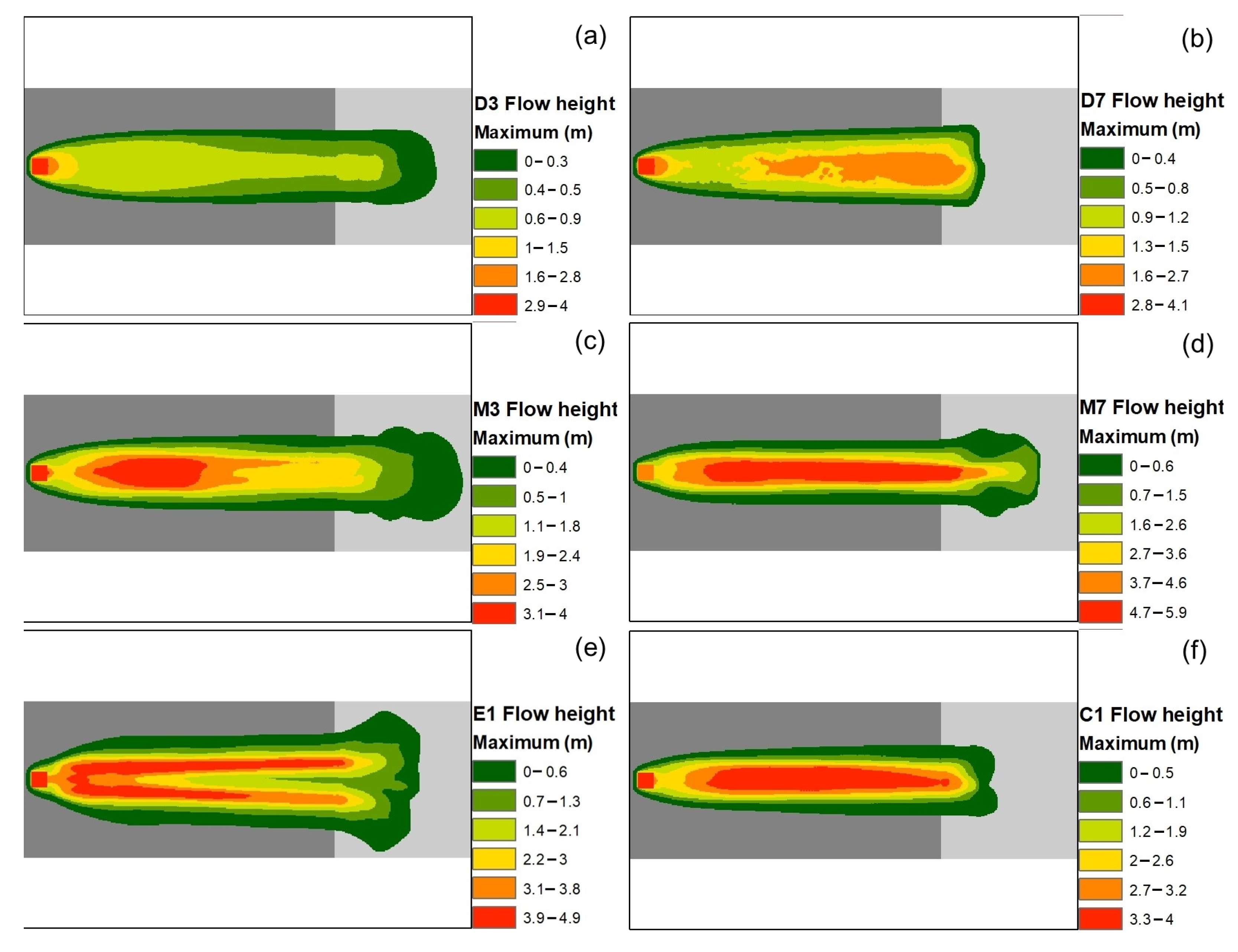
The maximum height of a flow is an important parameter to understand the flow behavior. It is also useful in identifying the critical locations in a field mass flow event. The top view of the maximum height of flows for extreme cases with minimum and maximum fluid content for each debris and mudflows, earthflow, and complex flow is shown in Figure 9. The maximum height is observed along the centerline of the flow in all the cases except the earth flow where the fine solid forms fingerlike shapes along with the flow due to lateral spreading. The height of flow reduces away from the centerline of the flow in all cases except in earthflow. It is also evident that the maximum heights of flows with low fluid content and high solid or fine solid fraction are greater. Due to the less longitudinal deformation in mudflow cases, their maximum heights cases are significantly higher compared to the debris flow cases, and they can maintain very large height after traveling a long distance, whereas the height of debris flows declines rather rapidly.
4.3. Run-Out Distance
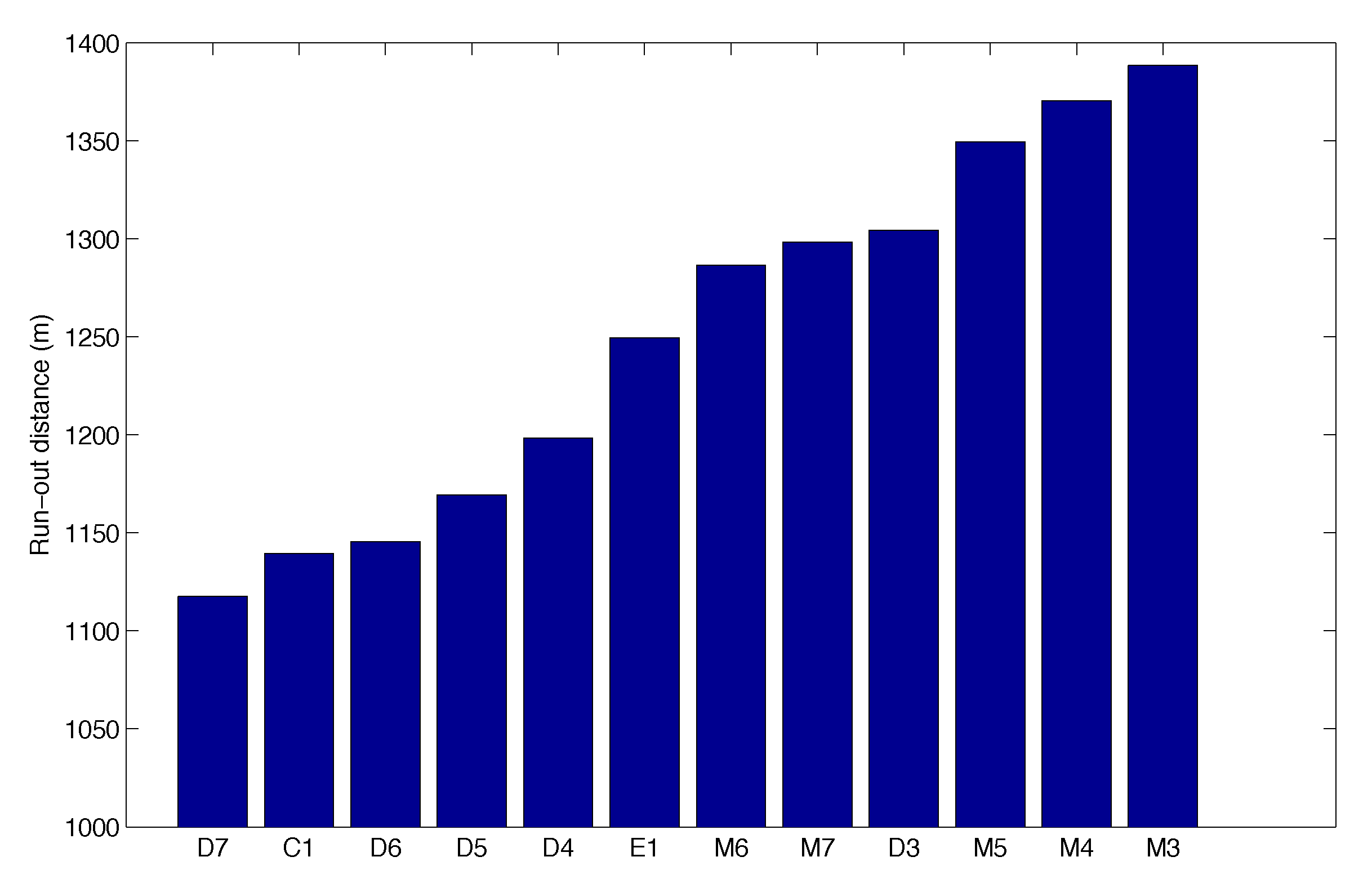
The total run-out distance is one of the most important physical parameters in the risk assessment of mass flows, as it delineates the critical location range susceptible to the major effect of potential mass flow events. The run-out distance is the total horizontal distance covered by the mass flow from its initiation to the final deposition. In the present study, the total run-out distance for each studied cases is presented in Figure 10, which shows the results of all cases in ascending order.
The results suggest that the run-out distance depends considerably upon the bed friction angle and the fluid content. The maximum run-out distance of 1355 m is observed in the M3 case; it is notable that this flow travels 405 m distance at the floor surface after the end of the slope on which a horizontal distance of 950 m is past by the mass flow. The D7 case with the high bed friction angle and low volume of fluid phase travels the minimum distance of 1084 m, which is 134 m from the end of the slope. The debris flow cases with high solid fractions associated with large bed friction angles generally travel shorter distances compared to the mudflow cases. In addition, cases with higher fluid volume also travel comparatively longer than solid- or fine solid- dominated flows. The analysis clearly suggests that the mass flows initiated by the rainfall events will have a long run-out distance due to a higher volume of the fluid phase. It is evident that the run-out distance also significantly depends upon the slope angle. It is worth noting that the earth flow (E1) with no fluid content travels farther than most of the debris flows, indicating overall the strong mobility of the visco-plastic fine solid phase.
4.4. Final Deposition
Final deposition thickness (or height) and its pattern are vital information reflecting the consequences of mass flows on the geomorphology. Final deposition is also crucially important for planning and evacuation purposes during disaster events, as deep deposition combined with large deposition area can be a very dangerous scenario and lead to heavy casualty and destruction of properties.
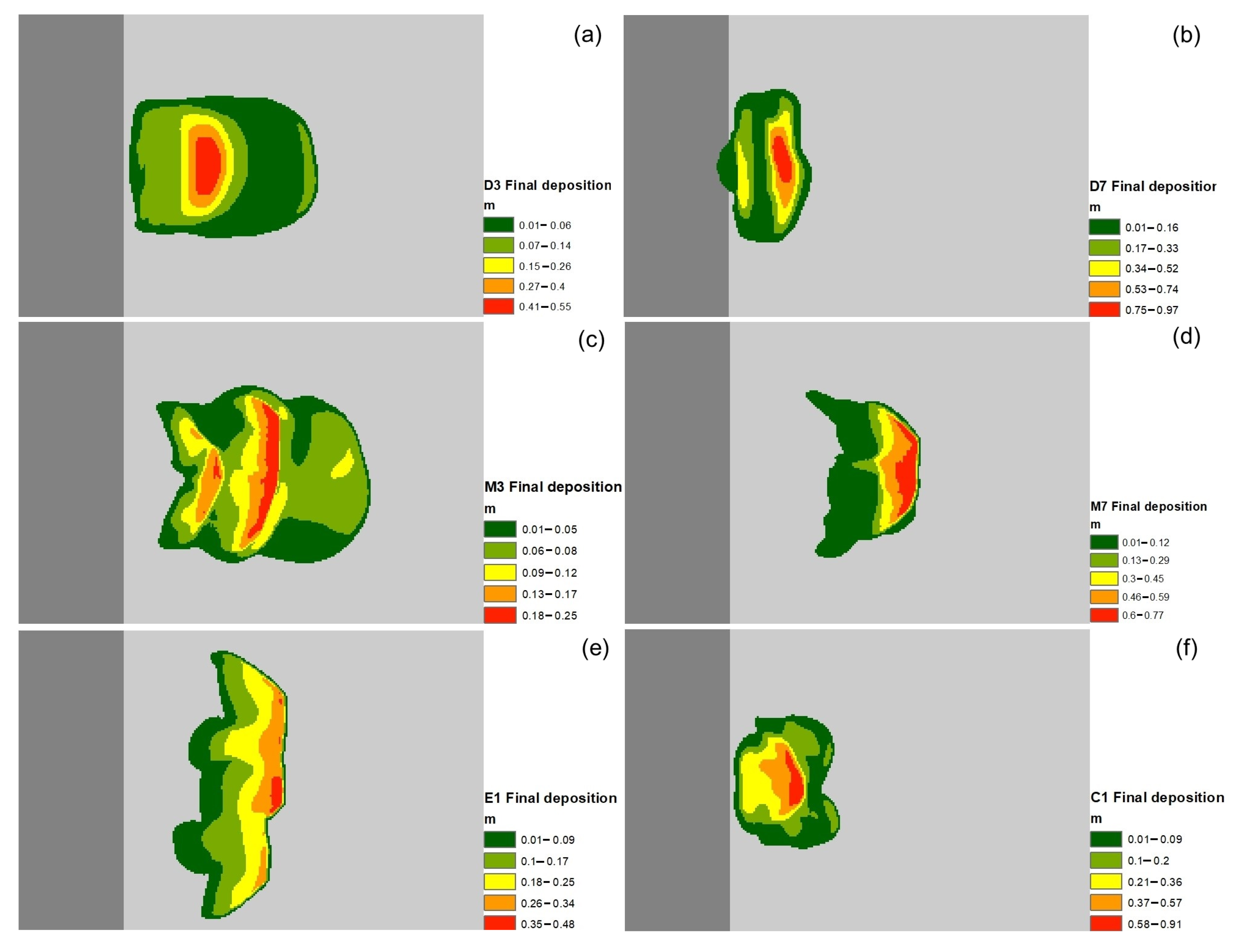
Various deposition patterns such as that concentrated on a smaller area with larger deposition height, or spread over a large area with a lower deposition height are evident in Figure 11. The maximum deposition area is observed in the M3 case, while the minimum area occurs in the C1 case followed by D7, both of which have a very modest fluid content. It is evident that flows with high fluid content deposit at a large area longitudinally while those with low fluid content expand laterally, because the mechanically weaker fluid phase offers low viscous resistance and travels greater distance compared to solid or fine solid phase, which stops earlier than the fluid. The maximum deposition height of approximately 0.97 m is found in the D7 case, which has a very high solid fraction; the maximum height is observed in the middle part of the deposited mass and decreases outwards. Overall, the deposition height in the M3 case seems smallest among the examined cases, as a result of a very low solid fraction.
4.5. Kinetic Energy
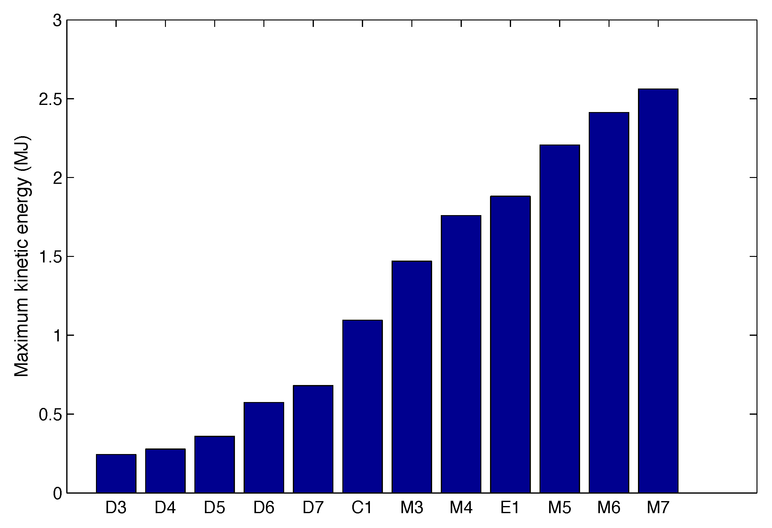
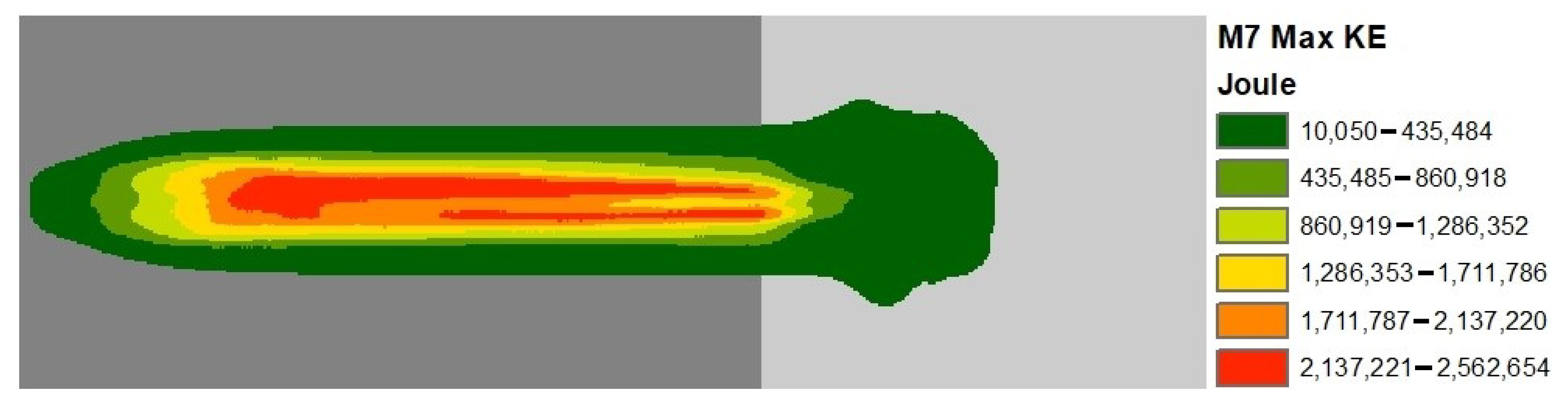
The maximum kinetic energy is calculated for all the cases and summarized in Figure 12. High kinetic energy can be associated with a higher destructive potential of landslides and pose a potential threat to infrastructure in the flow path, hence it is critically important for hazard risk assessment. The maximum kinetic energy is found to be significantly higher in mudflow cases compared to debris flow case, as shown in Figure 12, which shows the results for all cases in ascending order. The kinetic energy tends to increase with the increase in solid or fine solid ratio compared to the fluid phase. In the cases of mudflows, little longitudinal spreading of material during its propagation contributes to the maintenance of high kinetic energy. The maximum kinetic energy occurs in the M7 case with a magnitude of 2.562 MJ while the minimum is observed in the D3 case with a magnitude of 0.243 MJ. The highest kinetic energy in M7 case can be attributed to low basal roughness, low viscosity and presence of highly mobilized fluid phase. The distribution of maximum kinetic energy in the M7 case is shown in Figure 13. Evidently, the higher values of kinetic energy are dominant in the centerline of flow and decreasing outwards.
5. Concluding Remarks
The simulation of various mass flows is conducted based on a multi-phase computational framework. The cases representing debris flow, mudflow, earth flow, and complex flow are analyzed by varying the composition of various phases involved. Overall the simulated mudflow cases possess higher velocity, peak discharge, kinetic energy and longer run-out distance than the debris flow cases, presenting potentially greater danger or higher destructive forces under the examined scenarios. The fluid fraction significantly affects the flow dynamics; cases with high fluid content often result in higher velocity and longer run-out distance, but lower kinetic energy. The maximum velocity can reach more than 25 m/s, as observed in the M6 case, which can be classified as extremely rapid and possess high destructive potential. The evolution of the height of individual phases in a flow is very complicated and affected by the longitudinal and lateral spreading of each material phase. The debris flows have high longitudinal deformation while mudflows have higher lateral deformation. The final deposition and its pattern significantly depend on the fluid fraction. The phenomenon of fingering is observed in mudflow and earth flow cases.
The present study is primarily a parametric investigation that takes advantage of an available multi-phase computational framework for mass flows. The key model parameters such as internal and basal friction angle and kinematic viscosity have significant influence on the flow behavior and proper care should be taken when simulating the real world events using the actual field topographic data. The uncertainties associated with such large geotechnical systems of gravity-driven mass flows on a downslope are considerable; numerical simulations and relevant parametric studies may potentially provide quantitative results that help to assess the potential risks of destructive geological hazards or disasters.
Author Contributions
Conceptualization, M.W.N.; methodology, M.W.N., L.H.; software, M.W.N.; formal analysis, M.W.N.; investigation, M.W.N., D.K.; resources, L.H.; data curation, M.W.N., D.K.; writing—original draft preparation, M.W.N., L.H.; writing—review and editing, L.H.; visualization, M.W.N., D.K.; supervision, L.H.; project administration, L.H. All authors have read and agreed to the published version of the manuscript.
Funding
This research received no external funding.
Institutional Review Board Statement
Not applicable.
Informed Consent Statement
Not applicable.
Data Availability Statement
Data used in the present study is contained within the article.
Acknowledgments
The authors are grateful to Martin Mergili from University of Natural Resources and Life Sciences, Vienna, Austria, for assistance in the implementation of the numerical simulations with r.avaflow 2.0. The second author (D.K.) and third author (L.H.) wish to acknowledge the financial support provided by the University of Toledo through a Summer Research Fellowship during the preparation of this manuscript.
Conflicts of Interest
The authors declare no conflict of interest.
References
- Berger, C.; McArdell, B.W.; Schlunegger, F. Direct measurement of channel erosion by debris flows, illgraben, Switzerland. J. Geophys. Res. 2011, 346, F01002. [Google Scholar] [CrossRef] [Green Version]
- McCoy, S.W.; Kean, J.W.; Coe, J.A.; Tucker, G.E.; Staley, D.M.; Wasklewicz, T.A. Sediment entrainment by debris flows: In situ measurements from the headwaters of a steep catchment. J. Geophys. Res. 2012, 117, F03016. [Google Scholar] [CrossRef]
- Kjekstad, O.; Highland, L. Economic and Social Impacts of Landslides. In Landslides—Disaster Risk Reduction; Springer: Berlin, Germany, 2009; pp. 573–587. [Google Scholar]
- Ruttig, A.T. Slippery Slopes: Ecological, Social and Developmental Aspects of the Badakhshan Landslide Disaster. Available online: https://www.afghanistan-analysts.org/en/reports/economy-development-environment/slippery-slopes-ecological-social-and-developmental-aspects-of-the-badakhshan-landslide-disaste (accessed on 10 December 2021).
- Webb, S. Landslide in Indonesia Destroys Village, Killing 32–with 76 Still Missing and Hundreds Forced to Flee. Available online: https://www.dailymail.co.uk/news/article-2873232/Landslide-Indonesia-destroys-village-killing-24-84-missing-hundreds-forced-ee.html (accessed on 15 December 2021).
- Haque, U. Fatal landslides in europe. Landslides 2016, 13, 1545–1554. [Google Scholar] [CrossRef]
- Varnes, D. Slope movement types and processes. Natl. Acad. Sci. 1978, 176, 11–33. [Google Scholar]
- Hutchinson, J.N. General report: Morphological and geotechnical parameters of landslides in relation to geology and hydrogeology. In Proceedings of the Fifth International Symposium on Landslides, Rotterdam, The Netherlands, 10–15 July 1988. [Google Scholar]
- Hungr, O.; Evans, S.G.; Bovis, M.J.; Hutchinson, J.N. A review of the classification of landslides of the flow type. Environ. Eng. Geosci. 2001, 7, 221–238. [Google Scholar] [CrossRef]
- Hungr, O. Classification and Terminology BT—Debris-flow Hazards and Related Phenomena; Springer: Berlin/Heidelberg, Germany, 2005. [Google Scholar]
- Voellmy, A. Uber die zerstorungskraft von lawinen. Schweizerische Bauzeitung 1955, 73, 159–162. [Google Scholar]
- Cheng, C. Generalized viscoplastic modeling of debris flow. J. Hydraul. Eng. 1988, 114, 237–258. [Google Scholar] [CrossRef]
- Savage, S.B.; Hutter, K. The motion of a finite mass of granular material down a rough incline. J. Fluid Mech. 1989, 199, 177–215. [Google Scholar] [CrossRef]
- Hungr, O. A model for the run-out analysis of rapid flow slides, debris flows, and avalanches. Can. Geotech. J. 1995, 32, 610–623. [Google Scholar] [CrossRef]
- Iverson, R.M.; Denlinger, R.P. Flow of variably fluidized granular masses across three-dimensional terrain. J. Geophys. Res. Solid Earth 2001, 106, 553–566. [Google Scholar]
- Zahibo, N.; Pelinovsky, E.; Talipova, T.; Nikolkina, I. Savage-hutter model for avalanche dynamics in inclined channels: Analytical solutions. J. Geophys. Res. Solid Earth 2010, 115, 193–208. [Google Scholar] [CrossRef] [Green Version]
- Kowalski, J.; McElwaine, J.N. Shallow two-component gravity-driven flows with vertical variation. J. Fluid Mech. 2013, 714, 343–462. [Google Scholar] [CrossRef] [Green Version]
- Cesca, M.; D’Agostino, V. Comparison between FLO-2D and RAMMS in debris-flow modelling: A case study in the Dolomites. WIT Trans. Eng. Sci. 2008, 60, 197–206. [Google Scholar]
- Schraml, K.; Thomschitz, B.; Mcardell, B.W.; Graf, C.; Kaitna, R. Modeling debris-flow runout patterns on two alpine fans with different dynamic simulation models. Nat. Hazards Earth Syst. Sci. 2015, 15, 1483–1492. [Google Scholar] [CrossRef] [Green Version]
- Mitchell, A.; Zubrycky, S.; McDougall, S.; Aaron, J.; Jacquemart, M.; Hubl, J.; Kaitna, R.; Graf, C. Variable hydrograph inputs for a numerical debris-flow runout model. Nat. Hazards Earth Syst. Sci. 2020, 22, 1627–1654. [Google Scholar] [CrossRef]
- Guerriero, L.; Coe, J.A.; Revellino, P.; Grelle, G.; Pinto, F.; Guadagno, F.M. Influence of slip-surface geometry on earth-flow deformation, Montaguto earth flow, southern Italy. Geomorphology 2014, 219, 285–305. [Google Scholar] [CrossRef]
- Pudasaini, S.P.; Mergili, M. A multi-phase mass flow model. J. Geophys. Res. Earth Surf. 2019, 124, 2920–2942. [Google Scholar] [CrossRef] [Green Version]
- Pudasaini, S.P. A general two-phase debris flow model. J. Geophys. Res. Earth Surf. 2012, 117, F03010. [Google Scholar] [CrossRef]
- Domnik, B.; Pudasaini, S.P.; Katzenbach, R.; Miller, S.A. Coupling of full two-dimensional and depth-averaged models for granular flows. J. Non-Newtonian Fluid Mech. 2013, 201, 56–68. [Google Scholar] [CrossRef]
- Boetticher, A.V.; Turowski, J.M.; McArdell, B.W.; Rickenmann, D.; Kirchner, J.W. Debrisintermixing-2.3: A finite volume solver for three-dimensional debris-flow simulations with two calibration parameters—Part 1: Model description. Geosci. Model Dev. 2016, 9, 2909–2923. [Google Scholar] [CrossRef] [Green Version]
- Coussot, P.; Laigle, D.; Arattano, M.; Deganutti, A.; Marchi, L. Direct determination of rheological characteristics of debris flow. J. Hydraul. Eng. 1998, 24, 865–868. [Google Scholar] [CrossRef] [Green Version]
- Jop, P.; Forterre, Y.; Pouliquen, O. A constitutive law for dense granular flows. Nature 2006, 441, 727–730. [Google Scholar] [CrossRef] [Green Version]
- Pitman, E.B.; Le, L. A two-fluid model for avalanche and debris flows. Philos. Trans. R. Soc. 2005, 363, 1573–1601. [Google Scholar] [CrossRef]
- Jacobs, L.; Dewitte, O.; Poesen, J.; Delvaux, D.; Thiery, W.; Kervyn, M.A. The rwenzori mountains, a landslide-prone region? Landslides 2016, 13, 519–536. [Google Scholar] [CrossRef] [Green Version]
- Zhuang, J.Q.; Cui, P.; Peng, J.B.; Hu, K.H.; Iqbal, J. Initiation process of debris flows on different slopes due to surface flow and trigger-specific strategies for mitigating post-earthquake in old Beichuan County, China. Environ. Earth Sci. 2013, 68, 1391–1403. [Google Scholar] [CrossRef]
- Mergili, M.; Fischer, J.T.; Krenn, J.; Pudasaini, S.P. r.avaflow v1, an advanced open-source computational framework for the propagation and interaction of two-phase mass flow. Geosci. Model Dev. 2017, 10, 553–569. [Google Scholar] [CrossRef] [Green Version]
- Mergili, M.; Jaboyedoff, M.; Pullarello, J.; Pudasaini, S.P. Back calculation of the 2017 piz cengalo-bondo landslide cascade with r.avaflow: What we can do and what we can learn. Nat. Hazards Earth Syst. Sci. 2020, 20, 505–520. [Google Scholar] [CrossRef] [Green Version]
- Naqvi, M.W. Numerical Simulation of Debris Flows Using a Multi-Phase Model and Case Studies of Two Well-Documented Events. Master’s Thesis, University of Toledo, Toledo, OH, USA, 2020. [Google Scholar]
- Pudasaini, S.P. A full description of generalized drag in mixture mass flows. Eng. Geol. 2020, 265, 105429. [Google Scholar] [CrossRef]
- De Haas, T.; Braat, L.; Leuven, J.R.F.W.; Lokhorst, I.R.; Kleinhans, M.G. Effects of debris flow composition on runout, depositional mechanisms, and deposit morphology in laboratory experiments. J. Geophys. Res. Earth Surf. 2015, 120, 1949–1972. [Google Scholar] [CrossRef] [Green Version]
- De Haas, T.; Van Woerkom, T. Bed scour by debris flows: Experimental investigation of effects of debris-flow composition. Earth Surf. Process. Landforms 2016, 41, 1951–1966. [Google Scholar] [CrossRef] [Green Version]
- Iverson, R.M. The physics of debris flows. Rev. Geophys. 1997, 35, 245–296. [Google Scholar] [CrossRef] [Green Version]
Figure 1.
(a) Destruction caused by a debris flow in the Venezuelan town of Caraballeda (1999); courtesy of US Geological Survey. (b) Aerial shot of a post mudflow event at Montecito, USA (2018); courtesy of LA Times. (c) The Montaguto earth flow in Southern Italy (2006) [21].
Figure 1.
(a) Destruction caused by a debris flow in the Venezuelan town of Caraballeda (1999); courtesy of US Geological Survey. (b) Aerial shot of a post mudflow event at Montecito, USA (2018); courtesy of LA Times. (c) The Montaguto earth flow in Southern Italy (2006) [21].

Figure 2.
Geometry of the modeled slope.

Figure 3.
Velocity for all cases at two different locations.

Figure 4.
Velocity and height of individual phases at 30 s after flow initiation for (a) D3; (b) D5; (c) D7; (d) M3; (e) M5; (f) M7; (g) E1; (h) C1. The solid line represents the flow height and the bar chart the flow velocity.
Figure 4.
Velocity and height of individual phases at 30 s after flow initiation for (a) D3; (b) D5; (c) D7; (d) M3; (e) M5; (f) M7; (g) E1; (h) C1. The solid line represents the flow height and the bar chart the flow velocity.

Figure 5.
Flow discharge and height profile at 500 m from initial release for (a) D3; (b) D5; (c) D7; (d) M3; (e) M5; (f) M7; (g) E1; (h) C1. The solid line represents the flow height and the bar chart the discharge.
Figure 5.
Flow discharge and height profile at 500 m from initial release for (a) D3; (b) D5; (c) D7; (d) M3; (e) M5; (f) M7; (g) E1; (h) C1. The solid line represents the flow height and the bar chart the discharge.

Figure 6.
Flow discharge and height profile at 100 m away from the toe of the slope for (a) D3; (b) D5; (c) D7; (d) M3; (e) M5; (f) M7; (g) E1; (h) C1. The solid line represents the flow height and the bar chart the discharge.
Figure 6.
Flow discharge and height profile at 100 m away from the toe of the slope for (a) D3; (b) D5; (c) D7; (d) M3; (e) M5; (f) M7; (g) E1; (h) C1. The solid line represents the flow height and the bar chart the discharge.

Figure 7.
Top view for the height of flow for individual phases at 30 s for (a) D5: solid; (b) D5: fluid; (c) M5: fine solid; (d) M5: fluid; (e) E1: fine solid; (f) C1: solid; (g) C1: fine solid; (h) C1: fluid.
Figure 7.
Top view for the height of flow for individual phases at 30 s for (a) D5: solid; (b) D5: fluid; (c) M5: fine solid; (d) M5: fluid; (e) E1: fine solid; (f) C1: solid; (g) C1: fine solid; (h) C1: fluid.

Figure 8.
Top view for the height of flow for individual phases at 50 s for (a) D5: solid; (b) D5: fluid; (c) M5: fine solid; (d) M5: fluid; (e) E1: fine solid; (f) C1: solid; (g) C1: fine solid; (h) C1: fluid.
Figure 8.
Top view for the height of flow for individual phases at 50 s for (a) D5: solid; (b) D5: fluid; (c) M5: fine solid; (d) M5: fluid; (e) E1: fine solid; (f) C1: solid; (g) C1: fine solid; (h) C1: fluid.

Figure 9.
Maximum flowheight for (a) D3; (b) D7; (c) M3; (d) M7; (e) E1; (f) C1.

Figure 10.
Total run-out distance for all cases.

Figure 11.
Final deposition height in (a) D3; (b) D7; (c) M3; (d) M7; (e) E1; (f) C1.

Figure 12.
Maximum kinetic energy for all cases.

Figure 13.
Contours of maximum kinetic energy in M7.


Table 1.
Characteristics of several well-known flow types based on Hungr et al. [9].
Table 1.
Characteristics of several well-known flow types based on Hungr et al. [9].
| Name | Material | Water Content | Velocity |
|---|---|---|---|
| Earth flow | Clay or earth | Near plastic limit | Less than rapid |
| Debris flow | Debris | Saturated at rupture surface content | Extremely rapid |
| Mud flow | Mud | At or above liquid limit | Very to extremely rapid |
| Debris flood | Debris | Free water present | Extremely rapid |
| Debris avalanche | Debris | Partially or fully saturated | Extremely rapid |
| Rock avalanche | Fragmented Rock | Varied, mainly dry | Extremely rapid |
Table 2.
Notation for various analysis cases.
| Solid | Fine Solid | Fluid | |||||
|---|---|---|---|---|---|---|---|
| Flow | Initial | Initial | Initial | Initial | Initial | Initial | Notation |
| Type | Volume | Height | Volume | Height | Volume | Height | |
| Debris flow | 3000 | 1.2 | - | - | 7000 | 2.8 | D3 |
| 4000 | 1.6 | - | - | 6000 | 2.4 | D4 | |
| 5000 | 2.0 | - | - | 5000 | 2.0 | D5 | |
| 6000 | 2.4 | - | - | 4000 | 1.6 | D6 | |
| 7000 | 2.8 | - | - | 3000 | 1.2 | D7 | |
| Mudflow | - | - | 3000 | 1.2 | 7000 | 2.8 | M3 |
| - | - | 4000 | 1.6 | 6000 | 2.4 | M4 | |
| - | - | 5000 | 2.0 | 5000 | 2.0 | M5 | |
| - | - | 6000 | 2.4 | 4000 | 1.6 | M6 | |
| - | - | 7000 | 2.8 | 3000 | 1.2 | M7 | |
| Earth flow | - | - | 10,000 | 4.0 | - | - | E1 |
| Complex | 3333 | 1.33 | 3333 | 1.333 | 3333 | 1.33 | C1 |
Table 3.
Key parameters used in the numerical simulation.
| Parameter | Value |
|---|---|
| Solid | |
| Density | 2700 |
| Internal friction angle | |
| Basal friction angle | |
| Drag coefficient | 0.02 |
| Fine solid | |
| Density | 1800 |
| Internal friction angle | |
| Basal friction angle | |
| Kinematic viscosity | 10 |
| Fluid | |
| Density | 1000 |
| Kinematic viscosity | 0.001 |
| Fluid friction coefficient | 0.01 |
Publisher’s Note: MDPI stays neutral with regard to jurisdictional claims in published maps and institutional affiliations. |
© 2022 by the authors. Licensee MDPI, Basel, Switzerland. This article is an open access article distributed under the terms and conditions of the Creative Commons Attribution (CC BY) license (https://creativecommons.org/licenses/by/4.0/).
Share and Cite
MDPI and ACS Style
Naqvi, M.W.; KC, D.; Hu, L. Numerical Modeling and a Parametric Study of Various Mass Flows Based on a Multi-Phase Computational Framework. Geotechnics 2022, 2, 506-522. https://doi.org/10.3390/geotechnics2030025
AMA Style
Naqvi MW, KC D, Hu L. Numerical Modeling and a Parametric Study of Various Mass Flows Based on a Multi-Phase Computational Framework. Geotechnics. 2022; 2(3):506-522. https://doi.org/10.3390/geotechnics2030025
Chicago/Turabian StyleNaqvi, Mohammad Wasif, Diwakar KC, and Liangbo Hu. 2022. "Numerical Modeling and a Parametric Study of Various Mass Flows Based on a Multi-Phase Computational Framework" Geotechnics 2, no. 3: 506-522. https://doi.org/10.3390/geotechnics2030025