Coastal Flood Assessment due to Sea Level Rise and Extreme Storm Events: A Case Study of the Atlantic Coast of Portugal’s Mainland


1
Instituto Dom Luiz, Universidade de Lisboa, 1749-016 Lisboa, Portugal
2
Faculdade de Ciências, Universidade de Lisboa, 1749-016 Lisboa, Portugal
*
Author to whom correspondence should be addressed.
Geosciences 2019, 9(5), 239; https://doi.org/10.3390/geosciences9050239
Submission received: 3 May 2019
/
Revised: 17 May 2019
/
Accepted: 22 May 2019
/
Published: 24 May 2019
(This article belongs to the Special Issue Impacts of Compound Hydrological Hazards or Extremes)
Abstract
:Portugal’s mainland has hundreds of thousands of people living in the Atlantic coastal zone, with numerous high economic value activities and a high number of infrastructures that must be adapted and protected from natural coastal hazards, namely, extreme storms and sea level rise (SLR). In the context of climate change adaptation strategies, a reliable and accurate assessment of the physical vulnerability to SLR is crucial. This study is a contribution to the implementation of flooding standards imposed by the European Directive 2007/60/EC, which requires each member state to assess the risk associated to SLR and floods caused by extreme events. Therefore, coastal hazard on the Atlantic Coast of Portugal’s mainland was evaluated for 2025, 2050, and 2100 over the whole extension due to SLR, with different sea level scenarios for different extreme event return periods. A coastal probabilistic flooding map was produced based on the developed probabilistic cartography methodology using geographic information system (GIS) technology. The Extreme Flood Hazard Index (EFHI) was determined on probabilistic flood bases using five probability intervals of 20% amplitude. For a given SLR scenario, the EFHI is expressed, on the probabilistic flooding maps for an extreme tidal maximum level, by five hazard classes ranging from 1 (Very Low) to 5 (Extreme).
1. Introduction
Sea level rise, as consequence of global warming, has been occurring for more than a century. For a global temperature anomaly increase of around 1 °C, the global mean sea level (GMSL) has raised approximately 20 cm since the end of the 19th century, both globally and regionally [1,2,3,4]. Although there is a very low rate of regional uplifting, SLR on the west coast of Portugal’s mainland is in line with GMSL, with a slow and progressive response to global warming [5]. On one hand, this is due to the ocean’s thermal expansion and, on the other hand, yet to a smaller extent, to the ocean mass increase resulting from the melting of the continental glaciers and of the Greenland and Antarctica polar ice caps. However, the most recent data from the Gravity Recovery and Climate Experiment (GRACE) satellites’ mission and the Argo float network indicate that, since the beginning of this century, the ocean mass component increase has already surpassed the thermal expansion increase [4,6,7,8].
Due to the oceans’ well-known inertia, and with a slow response to global warming, SLR will continue to rise beyond the end of the 21st century. Even if global warming stops in the short term, the oceans would continue to rise due to the slow response of deep ocean warming and the melting dynamics of the glacier systems, either continental or Greenland and Antarctica.
We note the high exposure of the world’s population that live along coastal areas less than 10 m above mean sea level (MSL), representing around 10% of world population and 13% of urban population [9] with a higher share in the least developed countries (14%). In addition, there is the high importance of many types of infrastructure, namely, harbors and maritime transportation infrastructure, as well as economic activities, business, industry, tourism, and services (mainly in estuaries, deltas, and inlet areas). In the context of climate change, these two facts make the subject of SLR assessment a current and very important issue with strong socioeconomic impacts in the near future.
Through the Floods Directive 2007/60/EC [10], the European Parliament and Council of the European Union (EU) requires each member state to carry out a preliminary assessment to identify the river basins and associated coastal areas with a significant flooding risk due to climate change. For such zones, the member states must draw up flood risk maps and establish flood risk management plans focused on prevention, protection, and preparedness. The European Commission (EC) Directive applies to inland waters and all coastal waters across the whole territory of the EU.
Within the framework of this Directive’s requirements, the authors have been developing a methodology to produce coastal flood maps expressing the coastal flooding hazard resulting from the combination of SLR and extreme values of coastal forcing. The Atlantic Coast of Portugal’s mainland (ACPM) extreme flooding hazard assessment is crucial to producing the corresponding coastal vulnerability and risk cartography. Modeling several physical parameters, such as the tides measured in the Portuguese coastal harbors, the meteorological forcing factors, and the future SLR evaluation for 2050 and 2100, as well as the respective uncertainties, allows model coupling through a probabilistic approach and, consequently, the production of probabilistic flood hazard maps.
The ACPM coastal flood hazard assessment enables a wider physical vulnerability assessment at the national scale [11] and for regional case studies for inlet areas of estuary systems, such as the Ria de Aveiro (Northwest), the Tagus Estuary (Lisbon region) [12], and the Ria Formosa (South). These studies at the academic level, together with similar more detailed studies based on higher spatial resolution data (municipal service contracts), have contributed to the development of methodologies and algorithms to obtain final products such as coastal probabilistic flooding maps, investigated in this study, and coastal vulnerability and risk maps that will be published in the near future.
The present work describes the developed methodology to produce coastal flooding cartography for Portugal’s mainland considering extreme forcing and maximum high-water level. Flooding cartography is based on the most updated topographic model, without inferring any coastal profile morphodynamics nor considering coastline retreat due to present and future erosion. The difficulty and complexity of such coastal morphologic modeling, due to a variety of factors and constraints (of natural and human cause), would disable a country-wide high-resolution coastal risk assessment in such a limited time. The flooding cartography produced by the present methodologic approach is probabilistic rather than deterministic. Usually, the most common coastal flooding risk assessments use and apply flood hazard cartography based on a deterministic flood level [13,14,15,16]. However, Gesch [14] produces vulnerability maps with a linear error at 95% of confidence denoting a certain probabilistic approach. The reason why a probabilistic approach was applied to produce cartography is that the generated hazard maps serve to combine physical susceptibility and socioeconomic exposure maps to produce coastal risk maps on a standardized basis with five risk classes from 1 (low) to 5 (high). Moreover, this approach also reveals the areas that are most likely to be flooded due to SLR, which is important for territory management and planning concerning climate adaptation.
The developed methodology uses a hydrostatic flood model (usually called “bathtub model”) rather than a hydrodynamic flood model (computer-based dynamic water flow model), due to its simplicity when applying GIS technology and also because it does not require the use of an accurate high-resolution digital topo-bathymetric model, which is often not available at the national scale. Orton et al. [16] has demonstrated that the differences between hydrostatic and hydrodynamic models are moderate at the regional scale and large in a few locations for tropical cyclones, due to friction, wind, and other dynamic factors that affect the horizontal flood movement. However, the differences are small for extratropical cyclones, which is the case of most storms that reach the ACPM.
2. Materials and Methods
2.1. Coastal Flood Forcing
2.1.1. Sea Level Rise Projections
Data from the Cascais tide gauge (TG), the oldest gauge in Portugal and in the entire Iberian Peninsula and which has been working since 1882 (see [5] for the historical records), were used to estimate the first relative SLR empirical projection for the Portuguese coast by [17]. The gauge is located off the open coast, at a site of low tectonic activity [18] and reduced glacial isostatic adjustment (GIA) and with a sea level in considerable agreement with global SLR records [5].
Furthermore, Antunes [19], based on a daily average data series, concluded that the relative SLR at Cascais exhibited a rate of 4.1 mm/year for the past 12 years, demonstrating the correlation between the Cascais TG and GMSL rates. The Cascais SLR analysis validation was performed by comparing results with regional and global data models obtained from satellite and global tide gauge data, after removing the difference of the corresponding vertical velocity rate effect (obtained from tectonics and GIA) [5].
For different MSL data series and different methodological approaches, Antunes [5] showed a set of relative SLR projections for the 21st century, based on which the author generated a probabilistic ensemble used to compute an SLR probability density function at epoch 2100.
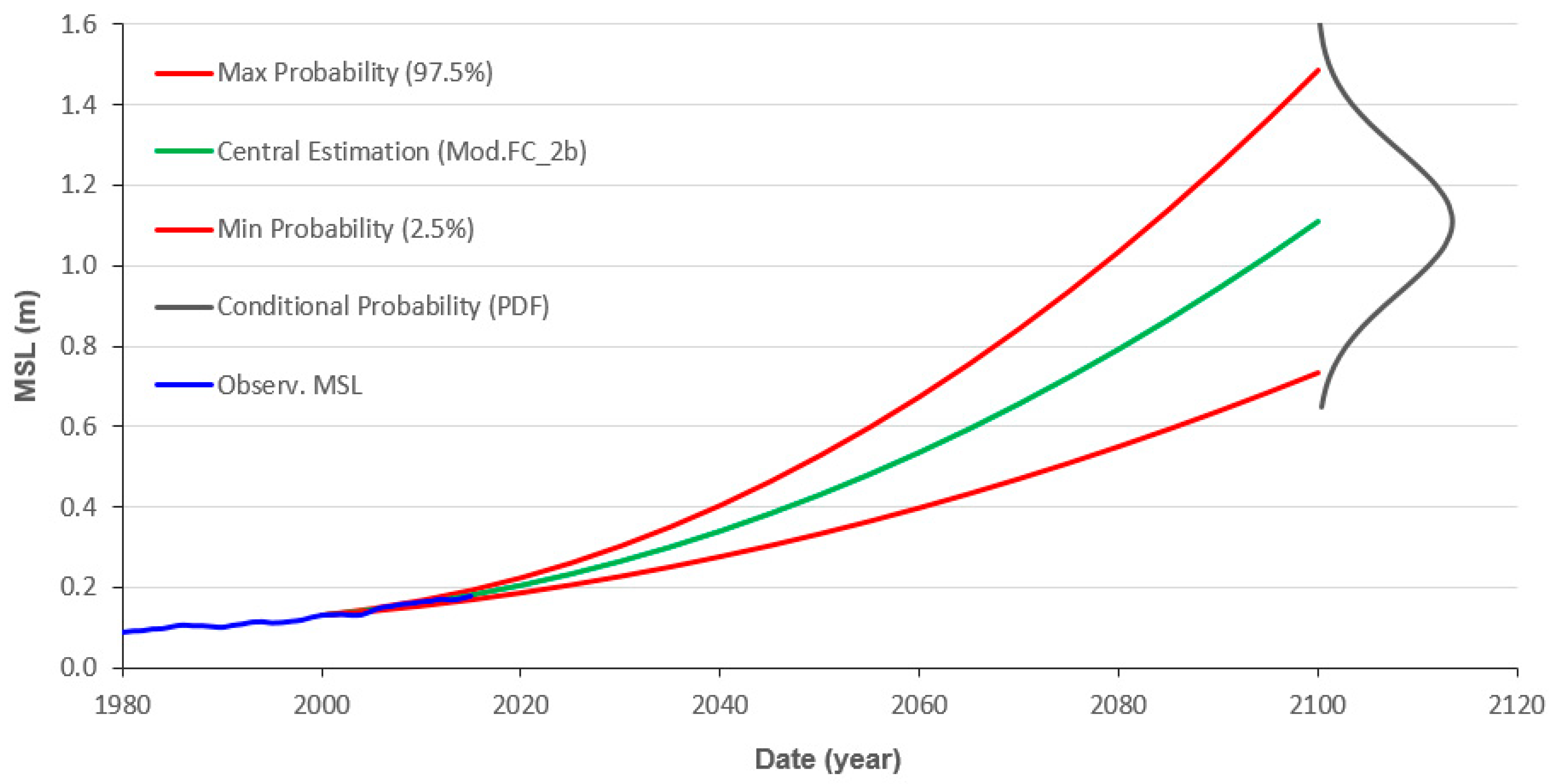
Based on the Cascais TG relative SLR estimation of 2.1 mm/year between 1992 and 2005 and 4.1 mm/year between 2006 and 2016, Antunes [5] estimated an accelerated SLR model, designated by Mod.FC_2b. The central estimate of this model (Figure 1) shows an intermediate hazard projection, when compared with other estimations and extreme values reported by Sweet et al. [4], with a value of 1.14 ± 0.15 m for epoch 2100. This Cascais TG projection model of SLR was applied to the entire ACPM to produce probabilistic coastal flood maps, used consequently for coastal vulnerability and risk assessment [10,11].
2.1.2. Maximum Tide Modelling
Longest tide series in Portugal are only available for the Cascais and Lagos TG, under the responsibility of the national Directorate-General for the Territorial Development (DGT). For the rest of the country, except for the Leixões harbor (North), the tides were only observed for short periods of a few years to two decades in the tide gauges under the responsibility of the Portuguese Hydrographic Institute (IH).
All tidal data, by convention, are referred to the vertical reference used in hydrography, the chart datum (CD), defined in Portugal as the lowest low-tide (minimum low water) observed during a period longer than 19 years (the Moon’s 18.6-year nodal period), plus an additional safety margin (one foot). For all Portuguese tide ports, the CD is 2.00 m relative to the national vertical reference, the 1938 Cascais Vertical Datum (CASCAIS1938), except for the Tagus Estuary, where the CD is 2.08 m. CD must be removed from the hydrographic tide heights to obtain the tide elevation, which corresponds to the tide orthometric height relative to the national vertical reference of CASCAIS1938.
Knowing that the maximum high tide has a synoptic variation of four to five years (one-quarter of the Moon’s nodal period), the annual reference tide for this study corresponds to a maximum high-water level, corresponding to the maximum of the equinoctial high tides. These maximum high tides occur when the Moon’s perigee is closer to the Earth (denominated “Giant Moon” or “Super Moon” years), causing the known “giant tides” or “king tides”. For this reason, the 2010 king tides were chosen for this national study.
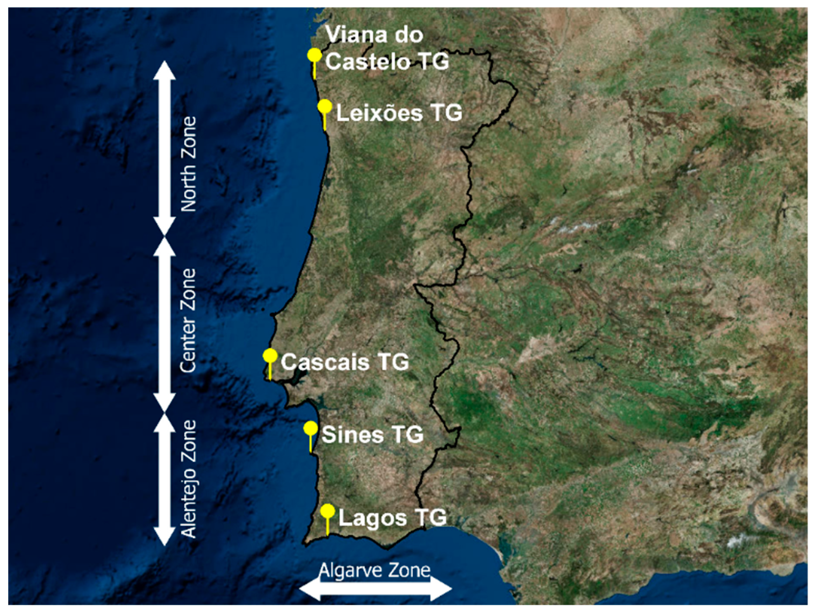
To enable a rapid and comprehensive assessment study, four tidal harbors, namely Leixões, Cascais, Sines, and Lagos, were chosen to estimate tides for the North, Center, Alentejo, and Algarve regions of the ACPM (Figure 2). This partition into four tidal zones, as it will be explained further, contributed also to the terrain data model simplification, enabling the entire coastal extension assessment using 20 m spatial resolution data without exceeding computing capacity demand.
Tide models from [20] were used to model four regional tides for the 2010 reference year, from which cumulative density functions (accumulated frequency or percentile function) were determined.
2.1.3. Storm Surge Modelling
Storm surge (SS) is the additional increase of the predicted astronomical tides caused by meteorological forcing due to storm events, through the joint effect of a lower atmospheric pressure, with a ratio of −1 cm/hPa, and the persistent effect of wind friction on the sea surface, depending on its direction and intensity. SS is a tide level disturbance, usually positive but which can also be negative when high atmospheric pressure occurs, ranging from a few centimeters to several meters, and which can last for hours to more than a day. In Portugal, according to an update study following the methodology of [21] that was based on the analysis of tide gauge data series from 1960 to 2018, the maximum observed storm surge along the west coast of Portugal’s mainland exhibited average values ranging from 50 to 70 cm for the different TGs, and maximum values of 80 cm to 1 m for long return periods (100 years or more). The maximum value detected by harmonic analysis was 82 cm in the Viana do Castelo TG (Figure 2) on October 15, 1987, and 83 cm in the Lagos TG on March 4, 2013. In the latter, such a magnitude is only explained by the additional wave setup effect due to the TG localization and the SW wave direction of the storm event.
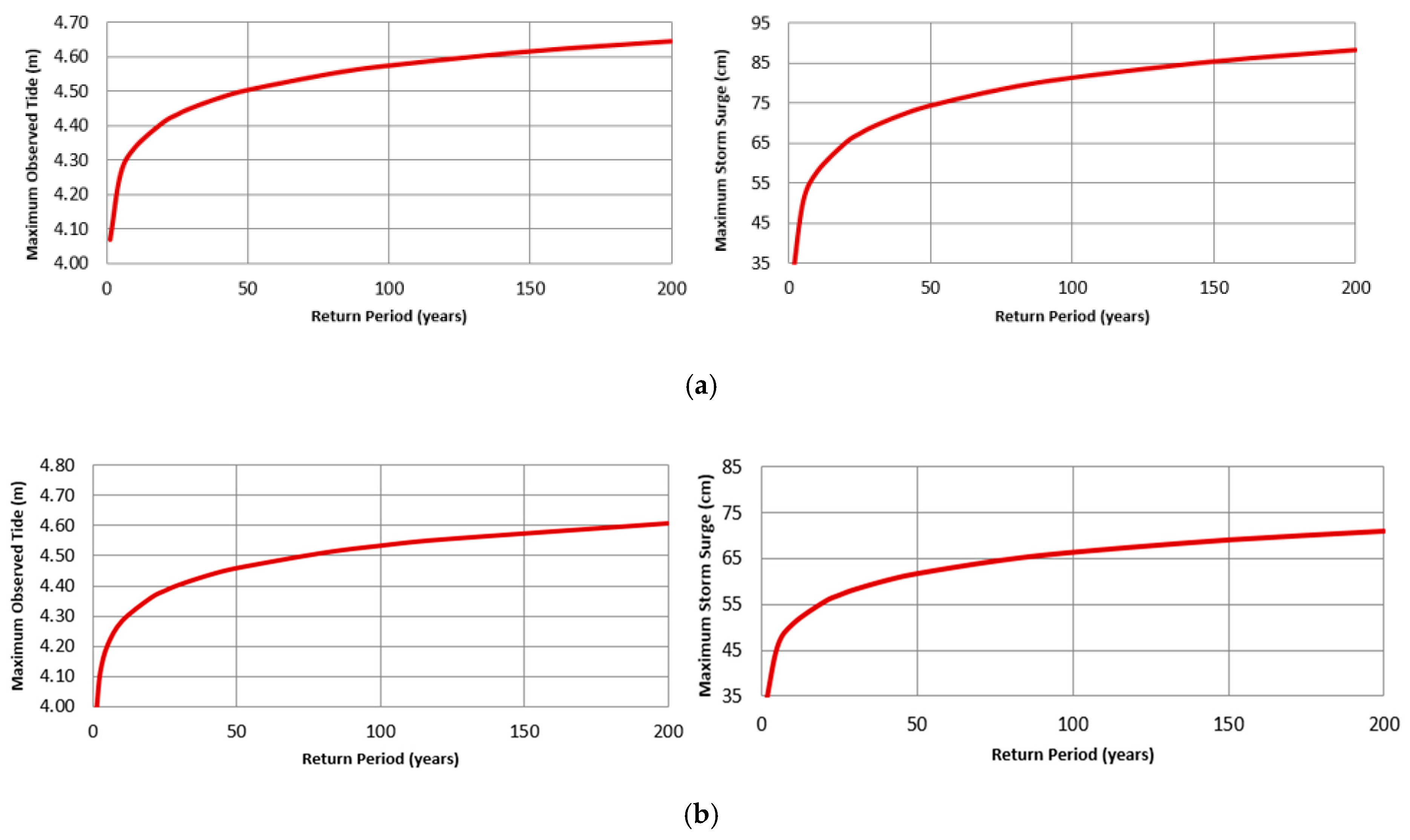
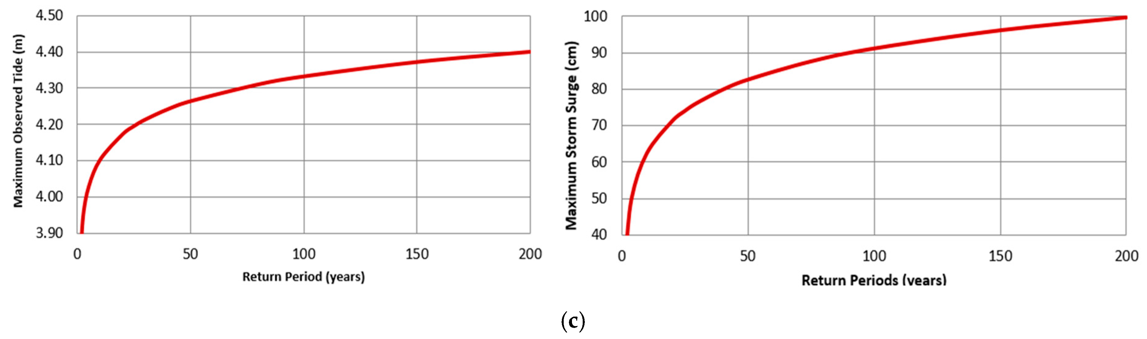
To evaluate and characterize the SS for the TG data series, a harmonic analysis was preformed, and the maximum storm surge series were updated for further analysis using the simple Gumbel distribution (Figure 3a–c).
The Viana do Castelo TG data set was used to assess the storm surge for the northern region (Figure 3a), due to the absence of enough data for the Leixões TG. The Cascais TG data set was applied for the central region storm surge assessment (Figure 3b), and the Lagos TG data set was used for the Alentejo and Algarve regions (Figure 3c).
With this characterization, the maximum tide frequency, corresponding to the maximum tide and extreme storm surge joint probability, the 50, 100, and 200-year return periods (RPs) were determined for the three TGs in the northern, central, and southern regions (Table 1).
2.1.4. Wave and Wind Setup
In addition to tide forcing and SS, sea level (SL) extremes are also influenced by the settling effect resulting either from coastal waves in the nearshore breaking zone or from strong winds, particularly in inland waters where swell waves do not reach. Thus, to estimate sea surface extreme values near the coast, the wave setup must also be considered for open sea coastal areas and the wind setup, for inland water areas (estuaries and coastal lagoons).
The model that was used for the wave setup () follows the direct integration method (DIM) applied by [22], which includes two setup components, namely, a static component () and a dynamic component , as follows:
The static component is given by the following:
where Hs is the significant wave height (highest third of the waves, H1/3). The dynamic component is defined by the combination of the setup oscillation standard deviation (σ1) and the incidence runup standard deviation (σ2), as follows:
where
and
where m is the average slope of the coast profile and Ts is the mean wave period.
The total effect of the wave setup coastal forcing corresponds to the overlapping of the incidence runup after the wave breaking. In this study, only average estimations of the wave setup component, without the addition of the incidence runup effect, were considered due to the impossibility of determining an accurate beach profile along Portugal’s mainland coastline.
Based on the wave record time series of the Leixões and Faro wave buoys, a maximum analysis was preformed using the Gumbel function. From this analysis, Hs and Ts, corresponding to RPs of 10 and 40 years (Table 2) of 6 and 7 m, were used for the calculation of the wave setup and added to the extreme tidal levels of 50- and 100-year RPs, respectively.
The wind setup Sv, applied only to inlets or inland waters, such as Ria de Aveiro and Ria Formosa (Algarve), and the Tagus Estuary, is obtained from the following expression [23]:
where V10 is the wind speed at 10 m above surface and ρw is the sea water density. Since no references were found for the region, an average wind speed of 38 km/h (10.6 m/s) was applied, resulting in the wind setup of Sv = 0.20 m.
2.2. Methodology for Coastal Flood Scenarios
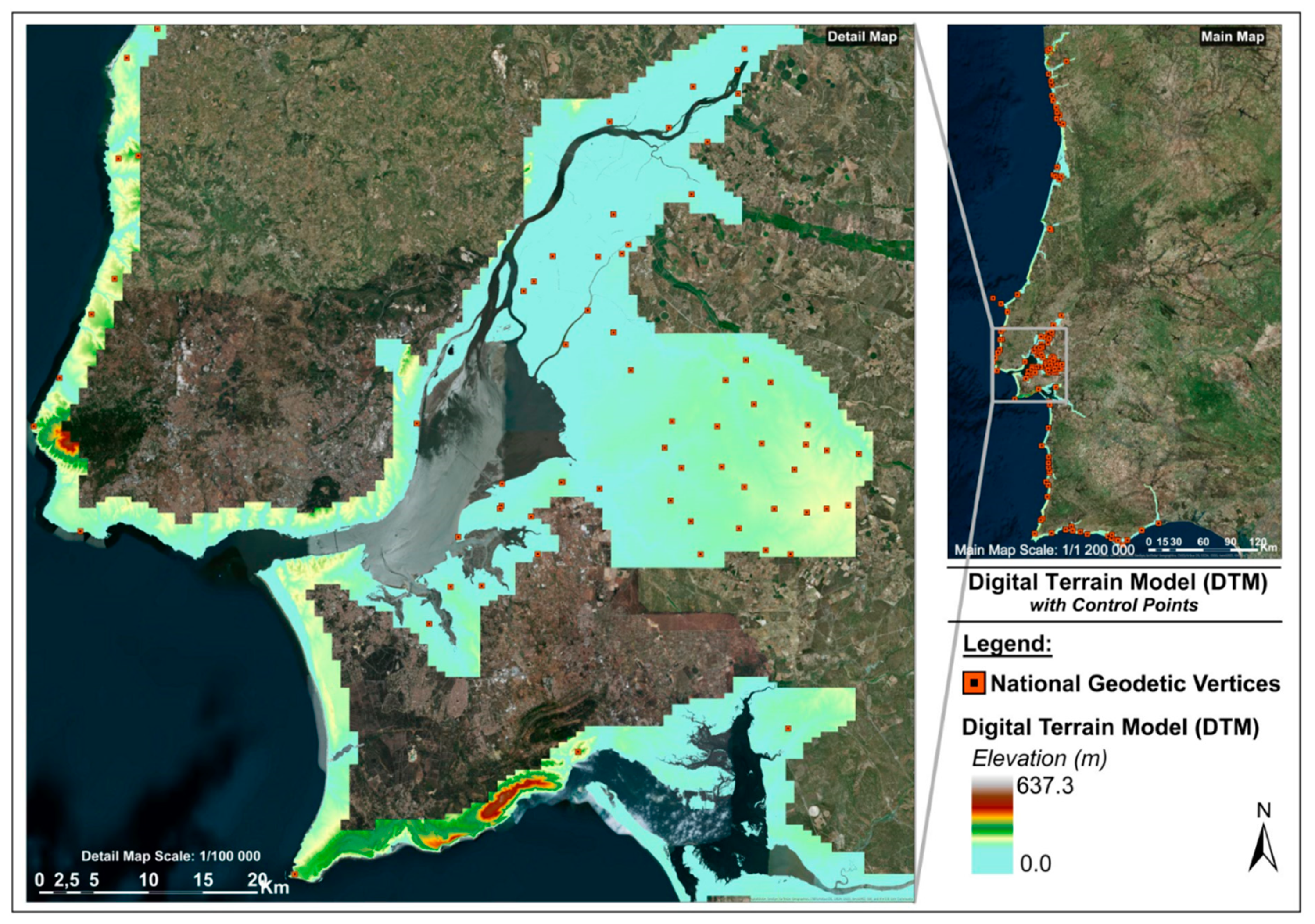
2.2.1. Digital Terrain Model
The Digital Terrain Model (DTM) used in this study was obtained from the photogrammetric model provided by the DGT. The aerial photogrammetric survey for the basic cartographic data acquisition along Portugal’s mainland coastal strip area, of approximately 513,400 ha, was carried out in 2008, with a spatial resolution of 2 m. In total, 4139 files of elevation points (X, Y, Z) were processed for the DTM calculation.
In order to improve the computational performance of altimetric data processing, four different geographical zones were separately considered and the corresponding altimetric grid resampled at 20 m spatial resolution (Figure 2): North (from Viana do Castelo to Figueira da Foz), Center (from Figueira da Foz to Cabo Espichel), Alentejo (from Sesimbra to Cabo de São Vicente) and Algarve (from Sagres to Vila Real Santo António) (Table 3). This partition became also an advantage for the coastal forcing computation, since there are different estimate scenarios for each zone with the combination of Portuguese Atlantic coast SLR and the respective tide model, SS, and wave setup estimations.
The positional quality control is indispensable in the production of flooding cartography due to the respective impact of an incorrect risk assessment. The DTM was produced by photogrammetry and, despite being a very efficient and accurate method, it is not free of errors. The respective data set was generated from raw data through filtering, by the classification of points into “soil” and “non-soil” and by interpolation to fill the gaps. Errors may still occur during post-processing of the data. Therefore, quality control should detect errors and deviations; however, it is very difficult to link certain errors (or their magnitude) to a concrete cause to be able to eliminate them [24].
In this regard, the validation of the DTM was done based on a set of ground control points, in a total of 134 national geodetic marks, for which the altimetric values (orthometric base height—HGV) are known and hence differences from the photogrammetric DTM heights (hDTM) can be estimated:
An overall mean square error of 56 cm was estimated with a sample of 134 control points for the entire coastal area. No shift, based on the obtained residual mean, was applied to the DTM, because the sample did not exhibit a normal random distribution due to the presence of large residuals. Finally, the obtained DTM (Figure 4), for the whole coastal zone of Portugal’s mainland, shows values between 0 m and 637.3 m with a spatial resolution of 20 m and with 56 cm of relative accuracy (precision).
2.2.2. Methodology for the Probabilistic Cartography
For the SLR hazard determination, vulnerability, and risk assessment, most of work done and published is based on the deterministic flooding cartography approach [13,14,15]. However, there are many unknowns when mapping future flood scenarios, including the evolution of coastal landforms (by erosion or sedimentation, or even man-made for building and protection), as well as the data used to produce the topographic models and to predict flooding levels. Partly based on the mapping confidence of [15], the present developed methodology is an innovative approach to produce the probabilistic cartography of different SLR scenarios, with different extreme event RPs and maximum tide levels.
Tide models were estimated based on historical data from the Leixões, Cascais, Sines, and Lagos TGs. Thus, each national wide scenario is a composition of four territorial zones: North, Center, Alentejo, and Algarve. Except for the Cascais TG, which has the longest tide series, all the other TGs (Leixões, Sines, and Lagos) have shorter and incomplete data series for the 1970–2010 period.
Considering the ACPM SLR projection (Figure 1) and the tide models, the tide submersion percentiles were computed for the two epochs under study, that is, 2050 and 2100. Adding the storm surge effect for two RPs considered (50 and 100 years), as well as wave setup, to the predicted tide level submersion frequency for each reference TG, the extreme flood levels (EFLs) are defined by the two Equations (8) and (9).
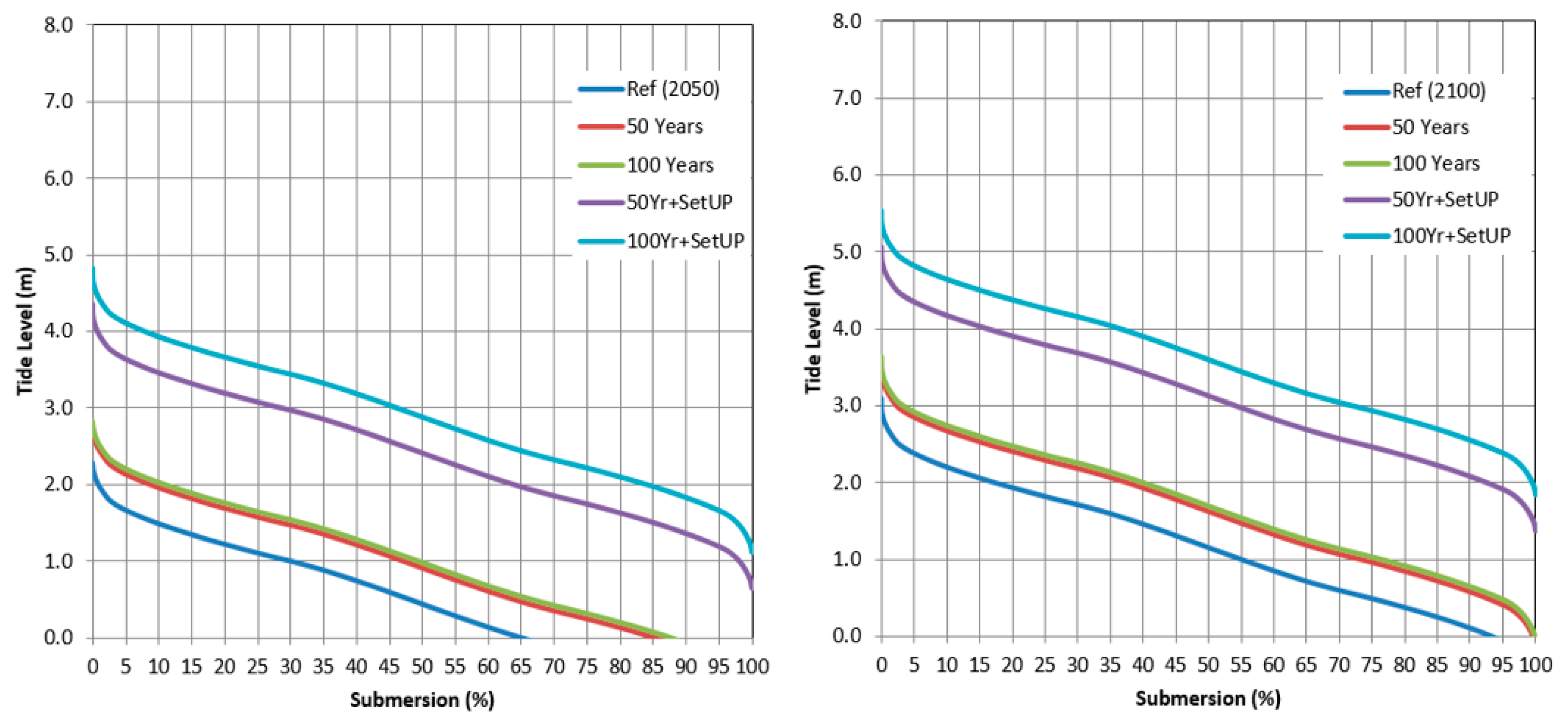
From the annual submersion percentile curve estimation, equivalent to the tide cumulative density function (shown in Figure 5 only for the case of Cascais, which is identical to the other TGs), the elevations for the extreme flooding levels (EFL central estimation) corresponding to the spring high-tide average were obtained using the 0.25% percentile of submersion tide level. From the percentile curves of Figure 5, for each EFL scenario, with or without additional storm surge and setup effects, the 0.25% percentile corresponds to an extreme tide level. With SLR, these extreme levels will cause flooding on coastal lowlands.
The developed probabilistic methodology for flooding cartography is mainly based on the uncertainties of the EFL unknowns, such as the SLR, prediction tide and storm surge uncertainties. Gesch [14] and Marcy et al. [15] used the same concept to produce the flooding map confidence, but only applying the uncertainty of the DTM. The present methodology could have also included the DTM uncertainty for the sake of a better probabilistic estimation. However, for this national case study only EFL uncertainties were considered, due mainly to the low confidence of the error mean square root estimation for the whole coastal DTM with only more than one hundred control points from the National Geodetic Network. Other studies, carried out at the local scale for the Portuguese municipality contracts, have considered the total uncertainties of the unknowns, including DTM with local control points. For this reason, one can say that the present EFL probability estimation and respective flooding cartography is underestimated.
The flooding hazard of a certain location for a given flood level increases with decreasing terrain height, since it returns higher water columns and higher flooding. On the other hand, due to the EFL uncertainty, the flooding occurrence probability in a certain location for a given flood level is also higher in terrain below EFL and lower in terrain above EFL. Therefore, contrary to the usual natural hazard probability, in which higher hazard has a low occurrence probability and vice versa (such as the storm surge or SLR itself), in this case high flooding hazard corresponds to a high occurrence probability and low flooding hazard corresponds to a low occurrence probability (Table 4).
To incorporate the EFL of each SLR scenario and their uncertainties (e.g., from Figure 1) into the further vulnerability and risk assessment, the Extreme Flood Hazard Index (EFHI) has been defined with five hazard classes (Table 4) ranging from 1 (low hazard with low probability) to 5 (extreme hazard with high probability). The EFHI is then calculated by considering the uncertainty of the submersion frequency models, which result from the tide standard deviation estimations of tides, storm surge RP, and SLR. Therefore, by variance propagation using Equations (8) and (9), the uncertainty of extreme flood scenario is evaluated by the following:
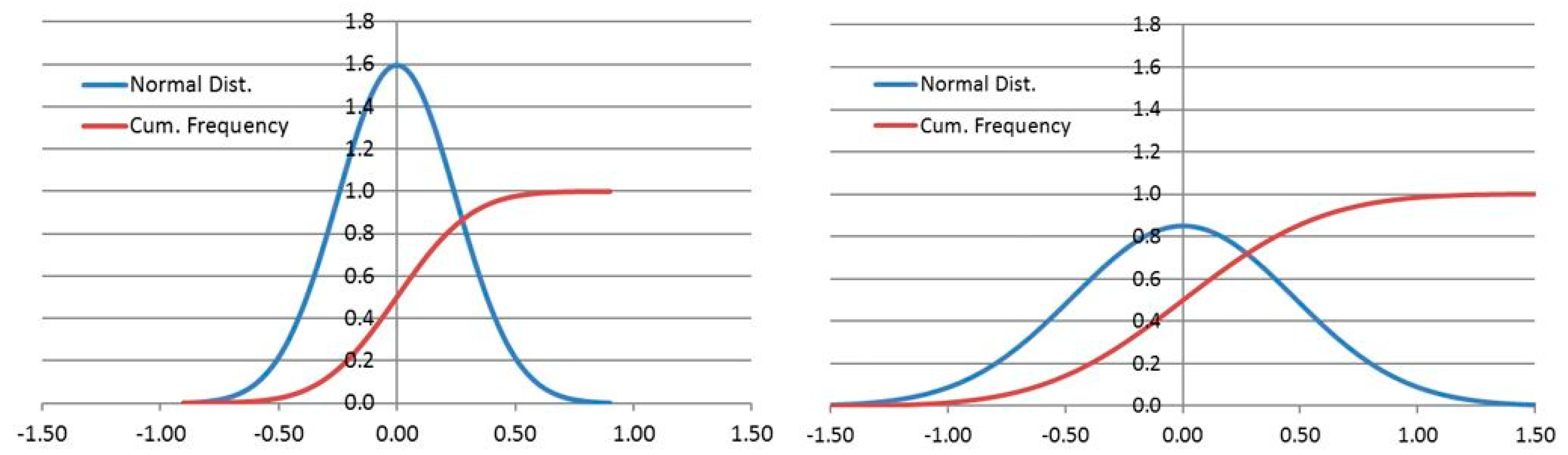
The uncertainty value of each scenario depends on the SLR projection epoch. Therefore, the scenario EFL1standard deviation values obtained for the 2050 and 2100 epochs were 12 and 40 cm, respectively. Based on these uncertainties estimated by Equation (10), the standard error distribution for a certain extreme flood scenario is determined (Figure 6).
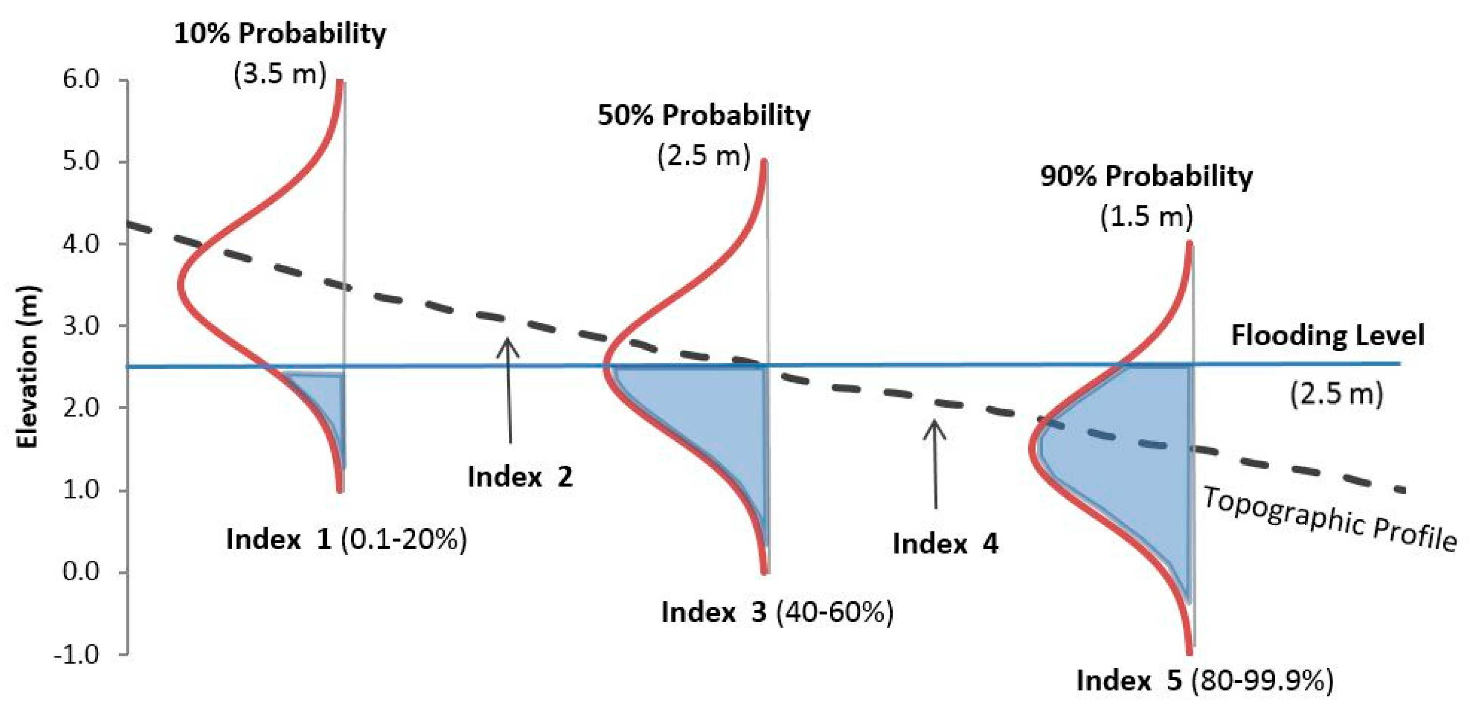
The respective standard error distribution being associated with the flooding level uncertainty should be centered at the EFL and intersected to the topographic profile to estimate the probability. However, the probability determined by such an approach would correspond to the given EFL exceeding probability at a certain topographic profile location. Therefore, instead of centering the respective normal distribution function at the EFL, it is centered rather at the topographic profile (Figure 7) to evaluate the EFL occurrence probability in a certain topographic location for a given flood level. Since the EFL is conditioned by a given SLR projection scenario, the respective probability corresponds to a conditional probability.
This normal distribution function has a conditional flood probability for the dimension of the topographic profile, which enables the determination of the probabilistic flood level for different topographic locations around the deterministic flood level (inundation level minus central projection of sea level). Subdividing the probability domain into five intervals of 20%, the EFHI is defined by a five-class range, from 1 (lowest probability, from 0.1 to 20%) to 5 (maximum probability, from 80 to 99.9%), related to coastal forcing (Table 4) and flooding hazard level.
3. Results
The costal flood hazard cartography is produced based in the GIS tools and supported by the most rigorous updated coastal DTM, referred to in Section 2.2.1. The flood hazard classification subdivided into five classes (from 1—Very Low Hazard to 5—Extreme Hazard) was then used to define the flooding scenario cartography, from which the coastal physical vulnerability model was further developed and evaluated [11]. The probabilistic flood cartography was only applied to the terrain model above MSL; therefore, water bodies such as the Tagus Estuary and the Aveiro and Faro inland lagoons were not considered in the flooded area due to the EFL.
3.1. Probabilistic Cartography of Coastal Flood
The flood scenario assessment presented here is based on a probabilistic rather than a deterministic approach as explained in Section 2.2.2 and is focused on the identification of areas with the flooding conditional probability for the future scenarios of SLR, for the time horizon of 2050 and 2100.
3.1.1. Year 2050
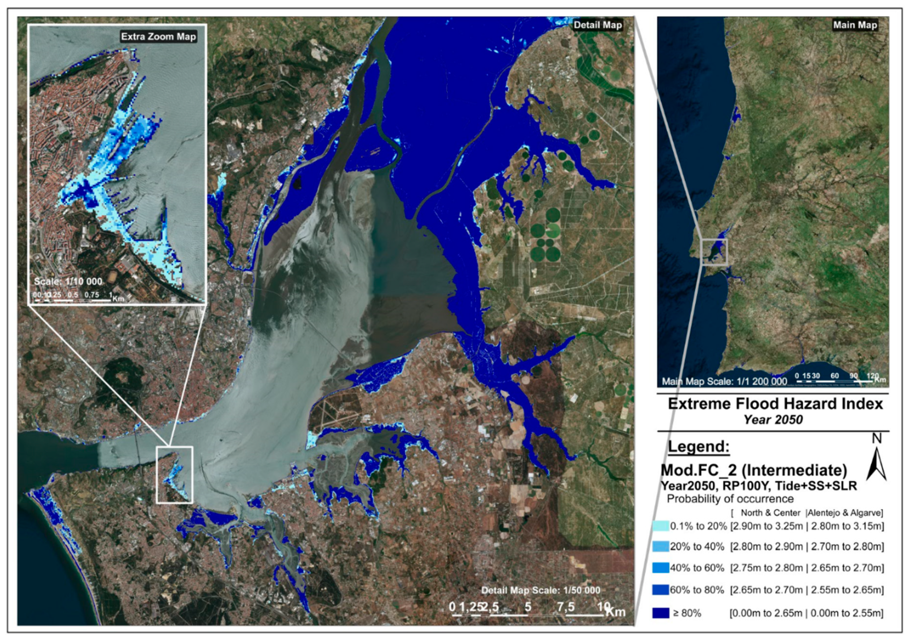
Table 5 shows the minimum and maximum values of each probabilistic interval corresponding to the five levels of flood hazard estimated for 2050. By intersecting these elevation interval levels with the DTM, the flooding areas for each scenario and geographical zone are obtained and classified into five classes of flooding hazard, represented by a given scale color in a GIS map visualizer.
Table 6 presents the amount of area (km2) for each hazard class and each Portuguese coastal district for the 2050 epoch. It is possible to see that 903.2 km2 of Portugal coastal zone are susceptible to flooding in an extreme scenario with 100-year RP and Lisbon being the district with the largest flooding area (221.4 km2), followed by the Faro district (182.4 km2). Although Santarém is not a coastal shoreline district, it is also affected by SLR scenarios due to the existence of the intertidal zone of the Tagus Estuary.
Figure 8 shows, for the ACPM, the 2050 coastal forcing scenario probability, within a zoom image of the Tagus Estuary and an extra zoom image of the Tagus southern margin at Cova da Piedade and Alfeite, in Almada municipality.
3.1.2. Year 2100
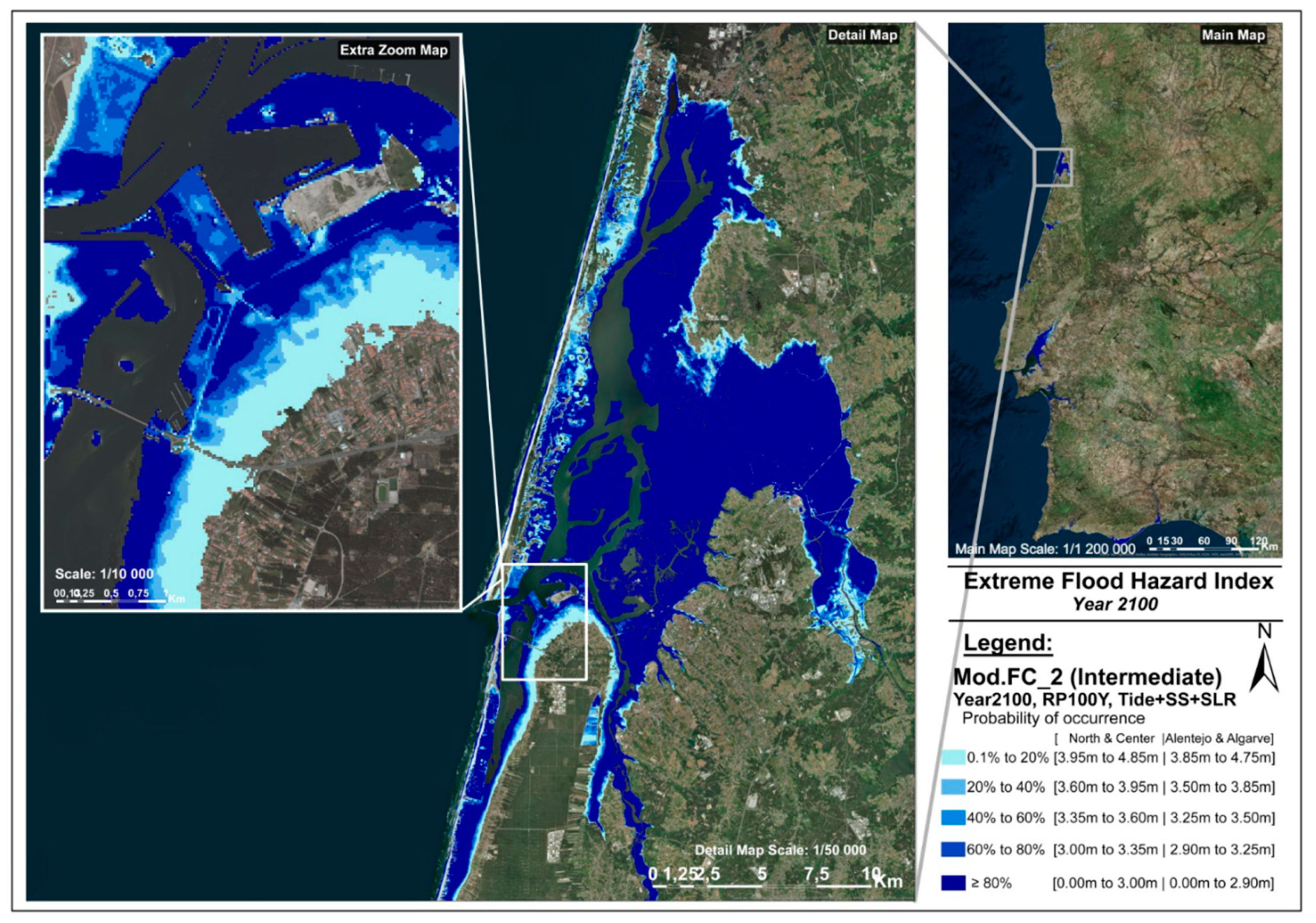
Table 7 shows the minimum and maximum values of each probabilistic interval corresponding to the five levels of flood hazard estimated for 2100.
Table 8 presents the sum of areas for each hazard class and each Portuguese coastal district for the 2100 epoch. In addition, it is also shown that an area of 1146 km2 has the probability of flood in 2100 and that 74.6% of that area is classified as extreme. The Lisbon district will be again the most affected with an area of 249.6 km2 with a probability of flood.
Figure 9 shows the 2100 coastal forcing scenario probability, within a zoom image of Ria de Aveiro lagoon and an extra zoom image of Gafanha da Narazé, in Ílhavo municipality, with the Aveiro commercial harbor.
3.2. Probabilistic Cartography of Extreme Coastal Flood with Wave and Wind Setup
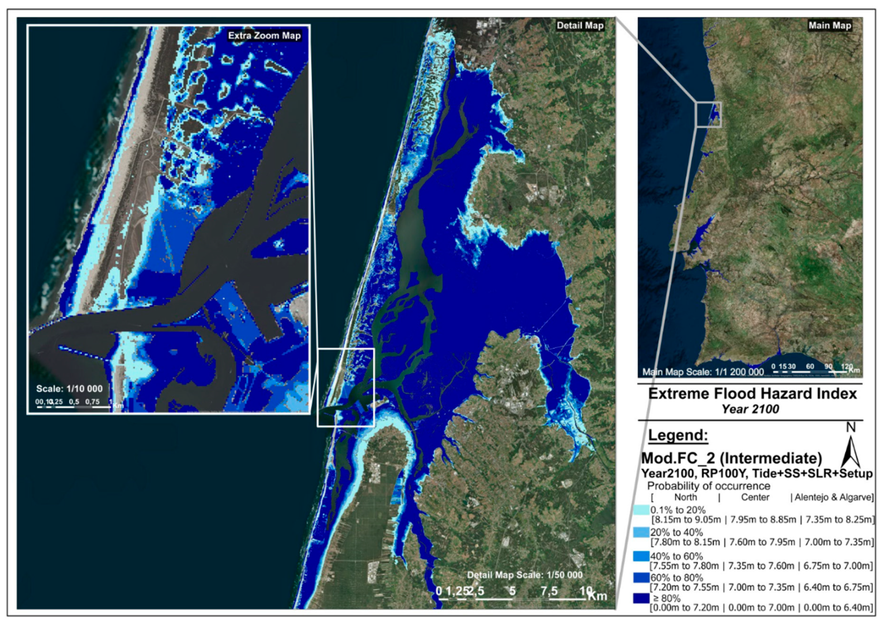
The extreme flood scenario with setup (EFL2 in Equation (9)) must be separated into open sea coastal areas (coastal shoreline), with the influence of ocean waves and consequently wave setup, and inland water areas, only influenced by wind setup, which requires a mask to apply both scenarios to the whole DTM in GIS.
Using the setup model values (wave setup presented in Table 2), Table 9 shows the minimum and maximum values of each probabilistic interval corresponding to the five levels of flood hazard estimated for 2100. For inland water zones, a maximum wind setup of 20 cm was added to the values in Table 7. The scenario uncertainty was kept the same (40 cm), due to the difficulty in estimating the respective coupled scenario standard deviation, knowing that the most accurate uncertainty would be higher than the one adopted and that the larger the flooded area would be.
Figure 10 presents, for the ACPM, the 2100 coastal forcing scenario probabilistic map with the additional wave and wind setup, with a detailed map of Ria de Aveiro and an extra zoom image of São Jacinto and the Aveiro harbor channel. Comparing Figure 9 with Figure 10, it is possible to observe some differences between them, specifically along the coastal shoreline and at the limits of the extreme arms of the lagoon. In the scenario with influence of wave and wind setup, there is a larger area with flooding probability, as it would be expected. This scenario is somehow realistic because storm surges can sometimes be accompanied by high energetic swell waves that generate a higher storm setup.
4. Conclusions
The developed methodology presents an innovative approach to produce coastal probabilistic flooding cartography for any considered SLR projection, any coastal force model coupling, and any DTM spatial resolution, based on a hydrostatic model and considering that the respective associated parameter uncertainties are provided or estimated.
Considering the Mod.FC_2b projection for the 2050 SLR with a SS of 50-yr RP for each TG zone, a total of 903 km2 of the ACPM is potentially affected by extreme flooding, the districts of Lisbon, Faro, and Aveiro being the most affected with 221, 182, and 172 km2 of flooded area, respectively. On the other hand, for 2100, those values rise to 1146 km2 of total area and 250, 211, and 219 km2, respectively, for the same most affected districts.
Knowing that the DTM represents the actual coastal morphology, without any erosion effect that is expected for future coastline retrieving, the present scenario for the coast shoreline with wave setup is underestimated. Due to the coastal retrieving, forced by the sedimentary deficit, the increase wave energy and its rotation caused by climate change, as well as the increasing effect of SLR on wave forward breaking towards inland, the flood extension and respective impact in open coast shoreline areas will be certainly much greater than what is estimated and presented in this study.
As is well known and widely studied, beach coastal areas are presently at high risk of erosion due to the sedimentary deficit and slightly increased wave energy coupled with SLR, but despite their economic and strategic importance, they are areas where the danger of SLR contributes less to the flooding vulnerability due to the low exposure of population and infrastructure, contrary to what is expected in the inland waters (river mouths, estuaries, and ocean water lagoons), where the much higher exposure will contribute potentially to a considerable higher risk level.
The probabilistic flood mapping production allows not only to quantify and qualify the flooded area hazard for each scenario, but also, through the formulation and classification of the EFHI combined with other physical susceptibility parameters, the future evaluation of the coastal vulnerability mapping and the coastal risk assessment. These outputs are and will be fundamental for coastal planning adaptation within a sustainable gradual and collaborative strategy.
Results contribute greatly to the identification of areas that are most vulnerable to SLR and extreme events in the context of climate change, not only because it is the first SLR flood assessment for all of Portugal’s mainland, but also because the coastal flooding risk is assessed and the Directive 20007/60/CE’s objectives are implemented.
Author Contributions
Conceptualization, C.A.; Data curation, C.R.; Formal analysis, C.A., C.R. and C.C.; Investigation, C.A. and C.R.; Methodology, C.A. and C.R.; Software, C.A., C.R. and C.C.; Supervision, C.A.; Validation, C.A., C.R. and C.C.; Visualization, C.R.; Writing–original draft, C.A. and C.R.; Writing–review & editing, C.A., C.R. and C.C.
Funding
This work was done under the framework of Portuguese Foundation for Science and Technology (FCT) project UID/GEO/50019/2019-Instituto Dom Luiz.
Conflicts of Interest
The authors declare no conflict of interest.
References
- Nerem, R.S.; Chambers, D.P.; Choe, C.; Mitchum, G.T. Estimating Mean Sea Level Change from the TOPEX and Jason Altimeter Missions. Mar. Geod. 2010, 33, 435–446. [Google Scholar] [CrossRef]
- Church, J.A.; White, N.J. Sea-Level Rise from the Late 19th to the Early 21st Century. Surv. Geophys. 2011, 32, 585–602. [Google Scholar] [CrossRef] [Green Version]
- Hay, C.C.; Morrow, E.; Kopp, R.E.; Mitrovica, J.X. Probabilistic reanalysis of twentieth-century sea-level rise. Nature 2015, 517, 481–484. [Google Scholar] [CrossRef] [PubMed]
- Sweet, W.V.; Kopp, R.E.; Weaver, C.P.; Obeysekera, J.; Horton, R.M.; Thieler, E.R.; Zervas, C. Global and Regional Sea Level Rise Scenarios for the United States. In NOAA Technical Report; NOAA: Silver Spring, MD, USA, 2017; NOS CO-OPS 083. [Google Scholar]
- Antunes, C. Assessment of sea level rise at west coast of Portugal Mainland and its projection for the 21st century. J. Mar. Sci. Eng. 2019, 7, 61. [Google Scholar] [CrossRef]
- Leuliette, E.W.; Scharroo, R. Integrating Jason-2 into a multiple-altimeter climate data record. Mar. Geol. 2010, 33 (Suppl. 1), 504–517. [Google Scholar] [CrossRef]
- Johnson, G.C.; Chambers, D.P. Ocean bottom pressure seasonal cycles and decadal trends from GRACE Release-05: Ocean circulation implications. J. Geophys. Res. 2013, 118, 228–240. [Google Scholar] [CrossRef]
- Roemmich, D.; Gilson, J. The 2004–2008 mean and annual cycle of temperature, salinity, and steric height in the global ocean from the Argo Program. Prog. Oceanogr. 2009, 82, 81–100. [Google Scholar] [CrossRef]
- McGrannahan, G.; Balk, D.; Anderson, B. The rising tide: Assessing the risks of climate change and human settlements in low elevation coastal zones. Environ. Urban. 2007, 19, 17–37. [Google Scholar] [CrossRef]
- European Parliament; Council of the European Union. Floods Directive (2007/60/EC); European Environment Agency: Copenhagen, Denmark, 2007; pp. 27–34. ISSN 1725-2555. [Google Scholar]
- Rocha, C.S. Estudo e Análise da Vulnerabilidade Costeira Face a Cenários de Subida do Nível do mar e Eventos Extremos Devido ao Efeito das Alterações Climáticas. Master’s Thesis, Faculdade de Ciências da Universidade de Lisboa, Lisboa, Portugal, 2016. [Google Scholar]
- Costa, M.S. Desenvolvimento de Uma Metodologia de Avaliação de Risco Costeiro Face aos Cenários de Alterações Climáticas: Aplicação ao Estuário do Tejo e à Ria de Aveiro. Master’s Thesis, Faculdade de Ciências da Universidade de Lisboa, Lisboa, Portugal, 2017. [Google Scholar]
- Poulter, B.; Halpin, P.N. Raster modelling of coastal flooding from sea-level rise. Int. J. Geogr. Inf. Sci. 2007, 1–16. [Google Scholar] [CrossRef]
- Gesch, D.B. Analysis of Lidar Elevation Data for Improved Identification and Delineation of Lands Vulnerable to Sea Level Rise. J. Coast. Res. 2009, 2009, 49–58. [Google Scholar] [CrossRef]
- Marcy, D.; Brooks, W.; Draganov, K.; Hadley, B.; Haynes, C.; Herold, N.; McCombs, J.; Pendleton, M.; Schmid, K.; Sutherland, M.; et al. New Mapping Tool and Techniques for Visualizing Sea Level Rise and Coastal Flooding Impacts. In Proceedings of the 2011 Solutions to Coastal Disasters Conference, Anchorage, AK, USA, 26–29 June 2011; pp. 474–490. [Google Scholar] [CrossRef]
- Orton, P.; Vinogradov, S.; Georgas, N.; Blumberg, A.; Lin, N.; Gornitz, V.; Little, C.; Jacob, K.; Horton, R. New York City Panel on Climate Change 2015 report chapter 4: Dynamic coastal flood modeling. Ann. N. Y. Acad. Sci. 2015, 1336, 56–66. [Google Scholar] [CrossRef] [PubMed]
- Antunes, C.; Taborda, R. Sea Level at Cascais Tide Gauge: Data, Analysis and Results. J. Coast. Res. 2009, 218–222. [Google Scholar] [CrossRef]
- Cabral, J. Neotectónica em Portugal Continental. Inst. Geol. Min. Mem. 1995, 31, 265. [Google Scholar]
- Antunes, C. Subida do Nível Médio do Mar em Cascais, revisão da taxa actual. In Proceedings of the 4as Jornadas de Engenharia Hidrográfica, Lisbon, Portugal, 21–23 June 2016; pp. 21–24, ISBN 978-989-705-097-8. [Google Scholar]
- Antunes, C. Previsão de Marés dos Portos Principais de Portugal. FCUL Webpage. 2007. Available online: http://webpages.fc.ul.pt/~cmantunes/hidrografia/hidro_mares.html (accessed on 3 May 2019).
- Vieira, R.; Antunes, C.; Taborda, R. Caracterização da sobreelevação meteorológica em Cascais nos últimos 50 anos. In Proceedings of the 2as Jornadas de Engenharia Hidrográfica, Lisbon, Portugal, 21–22 June 2012; pp. 21–24, ISBN 978-989-705-035-0. [Google Scholar]
- Federal Emergency Management Agency. Appendix D: Guidelines for Coastal Flooding Analysis and Mapping. In Guidelines and Specifications for Flood Hazard Mapping Partners; Federal Emergency Management Agency: Washington, DC, USA, 2002; Volume 3, Program Support; p. 384. [Google Scholar]
- Colvin, J.; Lazarus, S.; Splitt, M.; Weaver, R.; Taeb, P. Wind driven setup in east central Florida’s Indian River Lagoon: Forcings and pameterizations. Estuary Coast. Shelf Sci. 2018, 2013, 40–48. [Google Scholar] [CrossRef]
- Höhle, J.; Höhle, M. Accuracy assessment of digital elevation models by means of robust statistical methods. ISPRS J. Photogramm. Remote Sens. 2009, 64, 398–406. [Google Scholar] [CrossRef] [Green Version]
Figure 1.
Model of the relative SLR projection, Mod.FC_2b (Model 2b of Faculdade de Ciências da Universidade de Lisboa (FCUL)), based on the analysis of the Cascais tide gauge data series, from 1992 to 2016 [5], overlapped with observed mean sea level (MSL) at Cascais TG.
Figure 1.
Model of the relative SLR projection, Mod.FC_2b (Model 2b of Faculdade de Ciências da Universidade de Lisboa (FCUL)), based on the analysis of the Cascais tide gauge data series, from 1992 to 2016 [5], overlapped with observed mean sea level (MSL) at Cascais TG.

Figure 2.
Location of the five tide gauges (TGs) used in the study: Leixões, Cascais, Sines, and Lagos for the tide modeling and Viana do Castelo for storm surge analysis in the northern region.
Figure 2.
Location of the five tide gauges (TGs) used in the study: Leixões, Cascais, Sines, and Lagos for the tide modeling and Viana do Castelo for storm surge analysis in the northern region.

Figure 3.
Return period curves for the maximum observed tide (left), relative to the TG chart datum, and the maximum storm surge (right) for: (a) the Viana do Castelo TG (1978–2008 data series); (b) the Cascais TG (1959–2018 data series); (c) the Lagos TG (1986–2018 data series).
Figure 3.
Return period curves for the maximum observed tide (left), relative to the TG chart datum, and the maximum storm surge (right) for: (a) the Viana do Castelo TG (1978–2008 data series); (b) the Cascais TG (1959–2018 data series); (c) the Lagos TG (1986–2018 data series).


Figure 4.
Digital Terrain Model of the Atlantic Coast of Portugal’s mainland, with a spatial resolution of 20 m and 56 cm of relative accuracy estimated using the National Geodetic Network.
Figure 4.
Digital Terrain Model of the Atlantic Coast of Portugal’s mainland, with a spatial resolution of 20 m and 56 cm of relative accuracy estimated using the National Geodetic Network.

Figure 5.
Cascais tide submersion percentile for the reference mean sea level (MSL) (blue) at epoch 2050 (left) and epoch 2100 (right), with additional storm surge for 50- and 100-year return periods (red and green) and wave setup (purple and light blue).
Figure 5.
Cascais tide submersion percentile for the reference mean sea level (MSL) (blue) at epoch 2050 (left) and epoch 2100 (right), with additional storm surge for 50- and 100-year return periods (red and green) and wave setup (purple and light blue).

Figure 6.
Centered normal distribution and cumulative frequency of the 2050 (left) and 2100 (right) extreme flood levels (EFLs), corresponding to 12 and 40 cm of standard deviation, respectively.
Figure 6.
Centered normal distribution and cumulative frequency of the 2050 (left) and 2100 (right) extreme flood levels (EFLs), corresponding to 12 and 40 cm of standard deviation, respectively.

Figure 7.
Method for the flooding probability calculation and the EFHI on a generic topographic profile (3.5 m, 2.5 m, and 1.5 m), based on the highest tide level (h = 2.5 m) and its uncertainty (based in Marcy et al. rule for flood confidence area estimation [15]). Intermediate EFHI levels, 2 and 4, are located between index levels 1, 3, and 5, respectively.

Figure 8.
Portuguese coastal flooding extreme scenarios for 2050 SLR and 100-year RP, within a zoom image of the Tagus Estuary.
Figure 8.
Portuguese coastal flooding extreme scenarios for 2050 SLR and 100-year RP, within a zoom image of the Tagus Estuary.

Figure 9.
Portuguese coastal flooding extreme scenarios for 2100 SLR and 100-yr RP, within a zoom image of the Aveiro inland lagoon (Ria de Aveiro).
Figure 9.
Portuguese coastal flooding extreme scenarios for 2100 SLR and 100-yr RP, within a zoom image of the Aveiro inland lagoon (Ria de Aveiro).

Figure 10.
Portuguese coastal flooding extreme scenario with the influence of wave and wind setup, for 2100 SLR and 100-yr RP, within a zoom image of the Aveiro inland lagoon (Ria de Aveiro).
Figure 10.
Portuguese coastal flooding extreme scenario with the influence of wave and wind setup, for 2100 SLR and 100-yr RP, within a zoom image of the Aveiro inland lagoon (Ria de Aveiro).


Table 1.
Maximum tide height, relative to the respective TG chart datum, and storm surge (SS) for the 50-, 100-, and 200-year return periods, for the previous three TGs.
Table 1.
Maximum tide height, relative to the respective TG chart datum, and storm surge (SS) for the 50-, 100-, and 200-year return periods, for the previous three TGs.
| RP (Year) | Viana do Castelo | Cascais | Lagos | |||
|---|---|---|---|---|---|---|
| MaxTide (m) | SS (cm) | MaxTide (m) | SS (cm) | MaxTide (m) | SS (cm) | |
| 50 | 4.50 | 75 | 4.46 | 62 | 4.26 | 82 |
| 100 | 4.57 | 81 | 4.53 | 66 | 4.33 | 91 |
| 200 | 4.65 | 88 | 4.61 | 71 | 4.40 | 100 |
Table 2.
Significant heights (Hs) and mean wave periods (Ts), corresponding to the return period (RP) of 10 (line 1) and 40 years (line 2).
Table 2.
Significant heights (Hs) and mean wave periods (Ts), corresponding to the return period (RP) of 10 (line 1) and 40 years (line 2).
| Wave Height (Hs) (m) | Wave Period (Ts) (s) | Static Setup (m) | Dynamic Setup (m) | Total Setup (m) |
|---|---|---|---|---|
| 6.0 | 14 | 1.13 | 0.79 | 1.9 |
| 7.0 | 15 | 1.32 | 0.92 | 2.2 |
Table 3.
Number of elevation points for each geographical zone.
| Geographic Zone | Extension | No. of Elevation Points |
|---|---|---|
| North | Viana do Castelo to Figueira da foz | 3,069,154 |
| Center | Figueira da Foz to Cabo Espichel | 5,845,401 |
| Alentejo | Sesimbra to Cabo de São Vicente | 1,149,289 |
| Algarve | Sagres to Vila Real Santo António | 1,744,278 |
| Total | - | 11,808,122 |
Table 4.
Extreme Flood Hazard Index (EFHI) classification levels and respective conditional probability interval for an SLR scenario, relative to the respective central flooding elevation reference level (EFHI levels are related with color scale of hazard mapping, from 1—Light Blue to 5—Dark Blue).
Table 4.
Extreme Flood Hazard Index (EFHI) classification levels and respective conditional probability interval for an SLR scenario, relative to the respective central flooding elevation reference level (EFHI levels are related with color scale of hazard mapping, from 1—Light Blue to 5—Dark Blue).
| Hazard Class Level | Very Low | Low | Moderate | High | Extreme |
|---|---|---|---|---|---|
| 1 | 2 | 3 | 4 | 5 | |
| Flood Probability | 0.01–20% | 20–40% | 40–60% | 60–80% | >80% |
Table 5.
Intervals for each EFHI class and respective probability for the 2050 SLR scenario with 100-year RP storm surge for each geographic zone, relative to the central reference flooding elevation level (the Ref value corresponds to the EFL central estimation).
Table 5.
Intervals for each EFHI class and respective probability for the 2050 SLR scenario with 100-year RP storm surge for each geographic zone, relative to the central reference flooding elevation level (the Ref value corresponds to the EFL central estimation).
| Hazard Class Level | Flood Probability | North and Center | Alentejo and Algarve | ||
|---|---|---|---|---|---|
| Ref = 2.8 m | Ref = 2.7 m | ||||
| Min | Max | Min | Max | ||
| 1—Very Low | (0.1 to 20%) | 2.90 | 3.25 | 2.80 | 3.15 |
| 2—Low | (20 to 40%) | 2.80 | 2.90 | 2.70 | 2.80 |
| 3—Moderate | (40 to 60%) | 2.75 | 2.80 | 2.65 | 2.70 |
| 4—High | (60 to 80%) | 2.65 | 2.75 | 2.55 | 2.65 |
| 5—Extreme | (>80%) | 0.00 | 2.65 | 0.00 | 2.55 |
| Scenario uncertainty | 12 cm | ||||
Table 6.
Flooding areas (in km2) for each EFHI class interval and respective probability, for the 2050 SLR scenario in each coastal district.
Table 6.
Flooding areas (in km2) for each EFHI class interval and respective probability, for the 2050 SLR scenario in each coastal district.
| District | 1—Very Low (0.1 to 20%) | 2—Low (20 to 40%) | 3—Moderate (40 to 60%) | 4—High (60 to 80%) | 5—Extreme (>80%) | Total (km2) |
|---|---|---|---|---|---|---|
| Aveiro | 11.8 | 3.2 | 1.7 | 4.0 | 150.7 | 171.4 |
| Beja | 0.2 | 0.1 | 0.0 | 0.1 | 6.3 | 6.6 |
| Braga | 0.7 | 0.2 | 0.1 | 0.2 | 2.6 | 3.7 |
| Coimbra | 4.8 | 0.9 | 0.5 | 1.0 | 33.9 | 41.1 |
| Faro | 8.5 | 3.1 | 1.5 | 2.7 | 166.6 | 182.4 |
| Leiria | 3.5 | 0.9 | 0.5 | 1.1 | 14.2 | 20.2 |
| Lisbon | 12.3 | 4.1 | 2.4 | 5.8 | 196.8 | 221.4 |
| Porto | 0.4 | 0.1 | 0.0 | 0.1 | 1.9 | 2.5 |
| Santarém | 12.0 | 4.2 | 2.9 | 4.7 | 75.3 | 99.1 |
| Setúbal | 13.7 | 3.6 | 1.9 | 4.0 | 113.6 | 136.8 |
| Viana do Castelo | 2.8 | 1.1 | 0.4 | 0.9 | 12.7 | 17.9 |
| Total | 70.7 | 21.5 | 12.0 | 24.5 | 774.4 | 903.2 |
Table 7.
Intervals for each EFHI class and respective probability for the SLR 2100 scenario with 100-year RP storm surge for each geographic zone, relative to the central reference flooding elevation level (the Ref value corresponds to the EFL central estimation).
Table 7.
Intervals for each EFHI class and respective probability for the SLR 2100 scenario with 100-year RP storm surge for each geographic zone, relative to the central reference flooding elevation level (the Ref value corresponds to the EFL central estimation).
| Hazard Class Level | Flood Probability | North and Center | Alentejo and Algarve | ||
|---|---|---|---|---|---|
| Ref = 3.5 m | Ref = 3.4 m | ||||
| Min | Max | Min | Max | ||
| 1—Very Low | (0.1 to 20%) | 3.95 | 4.85 | 3.85 | 4.75 |
| 2—Low | (20 to 40%) | 3.60 | 3.95 | 3.50 | 3.85 |
| 3—Moderate | (40 to 60%) | 3.35 | 3.60 | 3.25 | 3.50 |
| 4—High | (60 to 80%) | 3.00 | 3.35 | 2.90 | 3.25 |
| 5—Extreme | (>80%) | 0.00 | 3.00 | 0.00 | 2.90 |
| Scenario uncertainty | 40 cm | ||||
Table 8.
Flooding areas (in km2) for each EFHI class interval and respective probability, for the SLR 2100 scenario in each coastal district.
Table 8.
Flooding areas (in km2) for each EFHI class interval and respective probability, for the SLR 2100 scenario in each coastal district.
| District | 1—Very Low (0.1 to 20%) | 2—Low (20 to 40%) | 3—Moderate (40 to 60%) | 4—High (60 to 80%) | 5—Extreme (>80%) | Total (km2) |
|---|---|---|---|---|---|---|
| Aveiro | 25.2 | 10.5 | 8.0 | 11.4 | 163.6 | 218.6 |
| Beja | 0.4 | 0.2 | 0.1 | 0.2 | 6.5 | 7.3 |
| Braga | 2.4 | 0.8 | 0.5 | 0.7 | 3.2 | 7.6 |
| Coimbra | 5.8 | 3.3 | 2.6 | 4.7 | 37.6 | 54.0 |
| Faro | 14.2 | 6.7 | 5.3 | 8.5 | 176.3 | 211.0 |
| Leiria | 7.1 | 3.3 | 2.4 | 3.5 | 17.8 | 34.1 |
| Lisbon | 10.5 | 8.2 | 6.6 | 11.2 | 213.2 | 249.6 |
| Porto | 2.0 | 0.6 | 0.4 | 0.4 | 2.2 | 5.7 |
| Santarém | 29.5 | 11.1 | 9.3 | 11.7 | 91.3 | 152.9 |
| Setúbal | 18.6 | 8.2 | 6.9 | 12.8 | 127.5 | 174.1 |
| Viana do Castelo | 7.1 | 3.1 | 2.1 | 2.9 | 15.9 | 31.1 |
| Total | 122.8 | 56.1 | 44.1 | 68.0 | 855 | 1146 |
Table 9.
Intervals for each EFHI level and respective probability for the SLR 2100 scenario with 100-year RP storm surge and the additional setup component for each geographic zone, relative to the central reference flooding elevation level (the Ref value corresponds to the EFL central estimation).
Table 9.
Intervals for each EFHI level and respective probability for the SLR 2100 scenario with 100-year RP storm surge and the additional setup component for each geographic zone, relative to the central reference flooding elevation level (the Ref value corresponds to the EFL central estimation).
| Hazard Class Level | Flood Probability | North | Center | Alentejo and Algarve | |||
|---|---|---|---|---|---|---|---|
| Ref = 7.7 m | Ref = 7.5 m | Ref = 6.9 m | |||||
| Min | Max | Min | Max | Min | Max | ||
| 1—Very Low | (0.1 to 20%) | 8.15 | 9.05 | 7.95 | 8.85 | 7.35 | 8.25 |
| 2—Low | (20 to 40%) | 7.80 | 8.15 | 7.60 | 7.95 | 7.00 | 7.35 |
| 3—Moderate | (40 to 60%) | 7.55 | 7.80 | 7.35 | 7.60 | 6.75 | 7.00 |
| 4—High | (60 to 80%) | 7.20 | 7.55 | 7.00 | 7.35 | 6.40 | 6.75 |
| 5—Extreme | (>80%) | 0.00 | 7.20 | 0.00 | 7.00 | 0.00 | 6.40 |
| Scenario uncertainty | 40 cm | ||||||
© 2019 by the authors. Licensee MDPI, Basel, Switzerland. This article is an open access article distributed under the terms and conditions of the Creative Commons Attribution (CC BY) license (http://creativecommons.org/licenses/by/4.0/).
Share and Cite
MDPI and ACS Style
Antunes, C.; Rocha, C.; Catita, C. Coastal Flood Assessment due to Sea Level Rise and Extreme Storm Events: A Case Study of the Atlantic Coast of Portugal’s Mainland. Geosciences 2019, 9, 239. https://doi.org/10.3390/geosciences9050239
AMA Style
Antunes C, Rocha C, Catita C. Coastal Flood Assessment due to Sea Level Rise and Extreme Storm Events: A Case Study of the Atlantic Coast of Portugal’s Mainland. Geosciences. 2019; 9(5):239. https://doi.org/10.3390/geosciences9050239
Chicago/Turabian StyleAntunes, Carlos, Carolina Rocha, and Cristina Catita. 2019. "Coastal Flood Assessment due to Sea Level Rise and Extreme Storm Events: A Case Study of the Atlantic Coast of Portugal’s Mainland" Geosciences 9, no. 5: 239. https://doi.org/10.3390/geosciences9050239
Note that from the first issue of 2016, this journal uses article numbers instead of page numbers. See further details here.