Influence of Sampling Methods on the Accuracy of Machine Learning Predictions Used for Strain-Dependent Slope Stability

Abstract

Supervised machine learning (ML) techniques have been widely used in various geotechnical applications. While much attention is given to the ML techniques and the specific geotechnical problem being addressed, the influence of sampling methods on ML performance has received relatively less scrutiny. This study applies supervised ML to the strain-dependent slope stability (SDSS) method for the prediction of the factor of safety (FoS) using hypoplasticity. It delves into different sampling strategies for training the ML model, emphasizing predictions of soil behavior in lower stress ranges. A novel sampling method is introduced to ensure a more representative distribution of samples in these ranges, which is challenging to achieve through traditional sampling approaches. The ML models were trained using traditional and modified sampling methods. Subsequently, slope stability analyses using SDSS were conducted with ML models trained from six different sampling methods. The results illustrate the impact of sampling methods on the FoS. Besides a noticeable improvement in predictions of shear stresses within the lower stress ranges, a decisive effect on the overall FoS was observed as well.

1. Introduction

Supervised machine learning (ML) methods like the artificial neural network (ANN) or multi-layer perceptrons (MLP) have been successfully applied to diverse geotechnical engineering problems. Examples of the application of supervised machine learning methods in geotechnics date back more than 25 years ago and include, for example, settlement estimation due to tunneling [1,2,3], the estimation of pile bearing capacity [4,5,6,7,8], foundation settlements [4,9], slope stability analysis [10,11,12], liquefaction potential assessment [4,13] and the adjustment of soil model properties to match field or experimental observations [14,15,16,17,18]. Among others, comparison and review of different ML algorithms has been conducted in [19,20]. The use of ANNs is primarily advantageous when the nature of the problem is complex and deals with uncertainties, where the empirical relations are not too accurate to the actual values.

Goh [4,21] described the ability of ANNs to predict the friction capacity of piles in clays. The input parameters considered for training included pile length, pile diameter, mean effective stress and undrained shear strength. Further, Goh [5,6] implemented ANN to estimate the ultimate load capacity of driven piles in granular soils. ANN provided better results compared to the common relationships for prediction of pile capacity. Later on, Lee and Lee [22] also implemented a neural network to predict the ultimate bearing capacity of piles. The results of the trained neural network were found to be in better agreement with the measured field values compared to the estimations from common analytical processes (Meyerhof’s equation [23]). These studies indicate the capacity and usefulness of ANNs to predict some outputs with higher accuracy than some known analytical/empirical procedures.

Goh [4] also developed a neural network for settlement prediction of a pile foundation in homogeneous soil. Sivakugan et al. [9] implemented ANNs to predict the settlement of shallow foundations on granular soils. The neural network was trained with five input parameters: net applied pressure, average blow count from SPT, shape, width and depth of foundation, and the actual observed settlement value was used for training the output. In this study, the ANNs were better at predicting foundation settlements than the classical analysis methods proposed by [24,25]. Similarly, Shahin et al. [26] implemented ANNs for settlement prediction of cohesionless soils. A total of 272 data records of actual settlement in cohesionless soil were used for training the ANN. The input variables included footing width, footing length, applied pressure on the footing, and soil compressibility. The results of this study confirmed that of [9], in the sense that ANNs outperformed the prediction of classical analysis methods. The classical analysis methods included [23,27,28].

Sakellariou and Ferentinou [11], Ferentinou and Sakellariou [12] analyzed the slope stability problem under monotonic and earthquake loading using ANNs for circular and wedge failure mechanisms. The model was trained with real information on 46 slopes composed of soil and 14 rock slopes. The ANNs successfully captured the relationship between input and output parameters. The authors also extracted information from the network by partitioning the connecting weights to study the dominance of the parameters on the FoS.

Puri et al. [29] studied the prediction of geotechnical parameters using ML techniques. The parameters such as in-situ density, compression index ($C_c$), cohesion (c) and angle of internal friction ($\phi$) were correlated with soil parameters determined in the laboratory and field. For example, c and $\phi$ were correlated with SPT N-value and $C_c$ was correlated with liquid limit and void ratio. The ML techniques implemented for that purpose included linear regression (LR), ANN, support vector machines (SVM), random forest (RF), and M5 tree (M5P). The training data were prepared from the geotechnical data collected from various government and private organizations. SVM produced the most accurate results for the prediction of $\phi$ based on SPT N-value, whereas, regarding c based on SPT N-value, M5P delivered the best predictions. M5P model was also the best performer for predicting $C_c$ using liquid limit and void ratio.

Wei et al. [30] implemented support vector regressor (SVR) models, in particular radial basis function (RBF) to predict the FoS for slope stability analysis based on different geotechnical parameters such as unit weight of soil within ($\gamma$), cohesion (c), angle of internal friction ($\phi$), slope inclination ($\beta$), pore water pressure coefficient ($r_u$), and slope height (H). The training data of the database consisted of 80 slope stability analyses carried out in existing literature. Different SVR models were used to evaluate the FoS. Among the employed SVR models, the RBF model was able to predict FoS with a very low error rate (RMSE = 0.076) and higher accuracy (R² = 0.947).

Nanehkaran et al. [31] studied the application of ML techniques for safety factor estimation in slope stability analyses. The performance of five different machine learning models, namely multilayer perceptron (MLP), k-nearest neighbor (kNN), support vector machines (SVM), decision tree (DT), and random forest (RF) to predict the slope safety factors were studied. The input data parameters included soil dry density, cohesion, friction angle, slope height and inclination. The output parameter was the factor of safety (FoS). The primary database source was a total of 70 slopes identified for slope stability analysis in South Pars region in southwest Iran. The slope stability was analyzed for each slope using the Limite Equilibrium Methods (LEM) prior to training. From the results obtained from the implemented machine learning models, it was concluded that the MLP was a superior classifier compared to the other four employed classifiers. Similarly, [32] performed a comparative analysis for slope stability using different ML techniques. The database for the study was prepared based on 100 records of soil slopes in Iran’s Fars, Isfahan, and Tehran provinces. The study concluded that MLP was able to predict the result with the highest accuracy (0.901), whereas kNN and DT also provided satisfactory results with accuracies greater than 0.8.

Schmüdderich et al. [33] suggested the application of machine learning techniques for the reduction of computational cost associated with the simulation of element tests within the framework of strain-dependent slope stability (SDSS) [34]. The method of SDSS is advantageous to other slope stability analysis methods due to its ability to accommodate any advanced constitutive model. However, it involves a lot of element test simulations to be performed, which demands a very high computational cost. This study investigated the replacement of the element test simulations by ML algorithms and tested the performance of MLP, kNN, RBF, and RF. The results of the ML algorithms were compared with the results obtained from the single element test simulations conducted using Incremental Driver [35]. The application of all four ML algorithms reduced the computational effort significantly while producing reasonably accurate results. However, the most preferable algorithm was considered to be RBF, while KNN produced a very fast but slightly less accurate evaluation. In the same study [33], the training data for the machine learning algorithms were prepared using a grid sampling approach. The results indicated that there was lower agreement between the Incremental Driver simulation results and the ML-trained models’ prediction for the test samples with lower initial effective stresses. However, whether this disagreement is due to the sampling approach or the machine learning algorithm itself remained unclear.

Most of the current studies regarding the application of ML techniques in geotechnics focus on the different machine learning algorithms, optimization strategies, and their accuracy. Explicit discussion of data sample preparation for training and its effect on the ML model performance is rare in geotechnical applications, mostly because algorithms can be easily used as black-boxes and the attention is focused on choosing the right set of controlling parameters that improve the quality of the prediction. However, the data sample preparation method is an important part of training any ML algorithm. The sampling technique plays a major role in the accuracy of prediction, as will be demonstrated in this research. A careful consideration of different sampling strategies ensures proper distribution of samples throughout the input parameter space. However, when complex constraints are needed in the model, the proper distribution of samples through the input parameter space becomes challenging. The present manuscript discusses the influence of sampling methods on the prediction results using ML algorithms and suggests techniques to ensure proper sampling distribution. The analysis is applied to the simulation of element tests as part of the strain-dependent slope stability method (SDSS). Two new sampling strategies are proposed to ensure a better distribution of samples in the input parameter space under the constraints of the failure surface and maximum and minimum void ratios employed as input parameters of the constitutive model. Finally, the proposed sampling strategies are applied to evaluate FoS using SDSS [34] and the influence of sampling strategies is discussed.

2. Enhanced Strain-Dependent Slope Stability Using Machine Learning

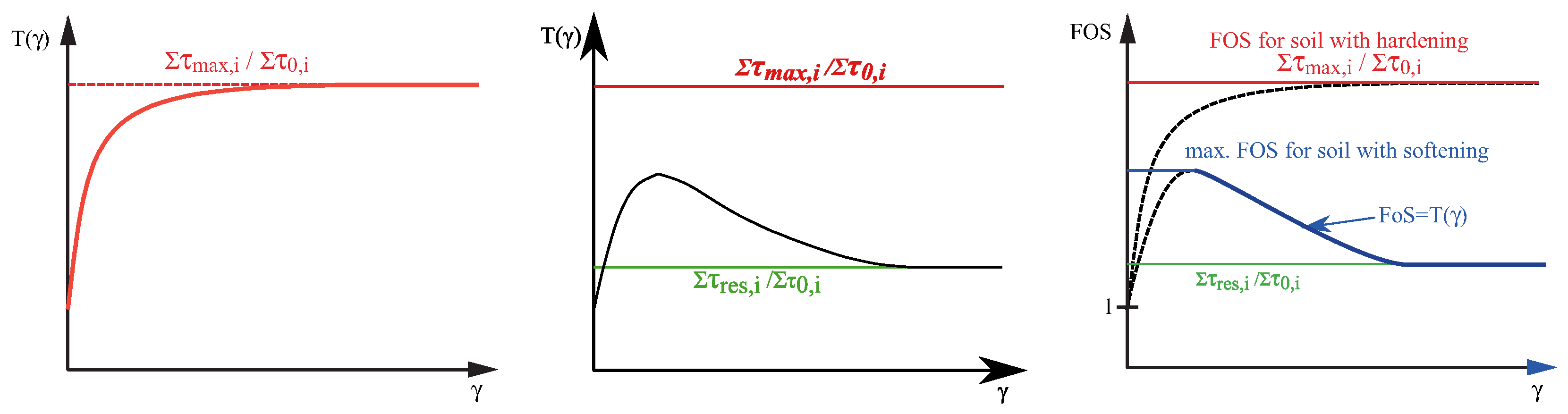
2.1. Strain-Dependent Slope Stability (SDSS)

Nitzsche and Herle [34] proposed the concept of strain-dependent slope stability where a calculation of the factor of safety can be performed considering a particular failure mechanism using FEM results with any constitutive model describing the soil behavior. A predefined slip surface is chosen and discretized into a number of segments using user-defined nodes. A predefined stress field is necessary (obtained by finite element simulations), so that the stresses for each node are interpolated and rotated in the direction of the predefined slip surface. The factor of safety is defined based on the mobilization of shear stresses considering the stress–strain behavior. The stress–strain behavior is simulated by performing a numerical element test (simple shear, triaxial or biaxial compression tests) for each node, which yields the evolution of shear stress mobilization with the increase in shear strains. The global mobilized shear resistance ratio $T\left(\gamma \right)$ for the particular slip surface is thus determined by the summation of the mobilized shear stresses ${\tau }_{\mathrm{mob}}$ with respect to the shear strain $\gamma$ along the nodes i, divided by the sum of initial shear stresses ${\tau }_0$ of each node i.

$$T\left(\gamma \right)={\displaystyle \frac{{\sum }_i{\tau }_{\mathrm{mob},i}\left(\gamma \right)}{{\sum }_i{\tau }_{0,i}}}$$

(1)

Equation (1) yields the global mobilized shear resistance T with respect to the shear strain $\gamma$, also depicted in Figure 1. Initially, $T\left(\gamma \right)=1$ since ${\sum }_i{\tau }_{\mathrm{mob},i}\left(\gamma \right)$ and ${\sum }_i{\tau }_{0,i}$ are equal, but then $T\left(\gamma \right)$ begins to increase with shearing. For loose soils with hardening behavior, $T\left(\gamma \right)$ approaches its maximum steady value when maximum shear strength is reached in all nodes. The corresponding value of the mobilized global shear resistance is expressed as ${\sum }_i{\tau }_{max,i}/{\sum }_i{\tau }_{0,i}$. For a loose soil, the FoS corresponds to this value. However, in the case of dense/stiff soils, $T\left(\gamma \right)$ initially increases until it reaches a peak value and then further decreases with ongoing shearing. At the final state, the shear stress in all nodes is equal to the critical shear strength. The mobilized shear stress $T_{\mathrm{mob},i}$ does not usually attain maximum values $T_{max,i}$ simultaneously at all nodes, causing the maximum value of $T\left(\gamma \right)$ to be smaller than ${\sum }_i{\tau }_{\max ,i}/{\sum }_i{\tau }_{0,i}$. Denoting $T_{max}$ as the maximum value of the global mobilized shear resistance obtained at a shear strain ${\gamma }_{max}$, the factor of safety (FoS) is calculated as follows [Figure 1 (right)]: ${\mathrm{FoS}}_{max}\left(\gamma \right)=T_{max}$ for $\gamma \le {\gamma }_{max}$ and $\mathrm{FoS}\left(\gamma \right)=T\left(\gamma \right)$ for $\gamma >{\gamma }_{max}$. In case of materials showing strain-softening behavior upon shearing, the maximum FoS corresponds to the maximum of $T\left(\gamma \right)$ and the residual FoS corresponds to ${\sum }_i{\tau }_{\mathrm{res},i}/{\sum }_i{\tau }_{0,i}$.

One of the significant advantages of SDSS over other slope stability analysis methods, such as LEM or the strength reduction finite element analysis, is the ability to consider advanced constitutive models (e.g., Hypoplasticity [36], Sanisand [37], Anisotropic Viscohypoplasticity [38] or AVISA [39]) for evaluation of the shear stress evolution, whereas other methods can incorporate only simple elastoplastic models such as Mohr–Coulomb, where the shear strength is controlled by the cohesion and friction angle. Apart from stress states, state and internal variables of the corresponding constitutive model obtained from the finite element simulation can be transferred to the numerical element test simulation. This indeed allows for better prediction of shear stress mobilization along the slip surface compared to other methods.

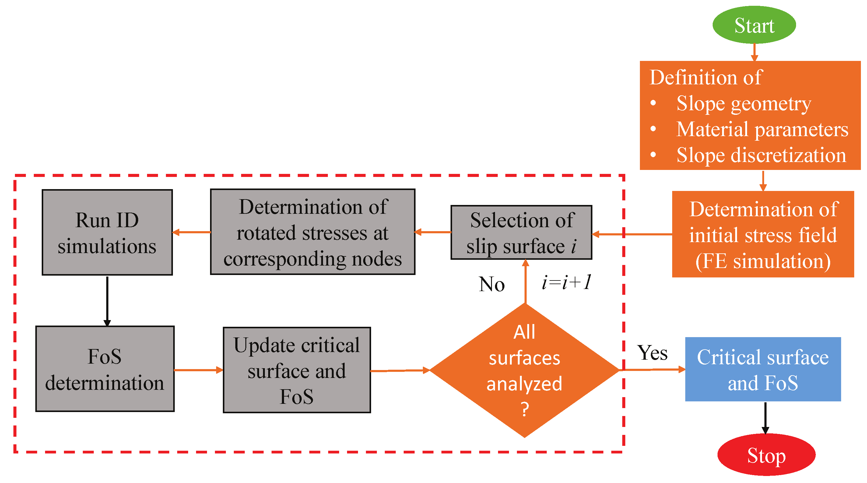
2.2. Implementation of SDSS

SDSS enables the evaluation of the FoS considering advanced constitutive models by performing element tests for nodes located along a potential slip surface. Different shapes of the slip surface can be used, such as planar or circular slip surface considering a translational or rotational failure of the soil above the slip surface, respectively. In this study, circular slip surfaces are used as planar surfaces tend to yield non-conservative results. The general workflow to detect the critical slip surface associated with the smallest FoS is depicted in Figure 2.

SDSS can be conducted on the basis of different element tests; for instance, direct simple shear (DSS) tests or a combination of DSS and triaxial compression tests. In this study, only DSS tests are considered. Element tests can be simulated using continuum finite elements or single Gauß point solvers. In this study, Incremental Driver [35] is utilized. Incremental Driver is a program for testing constitutive models, performing element tests that could be strain, stress or mixed controlled considering only a single Gauss point. The program requires the definition of the initial conditions, the constitutive model with its corresponding parameters and the testing program. The former is defined in terms of the initial stress state and the initial values of the internal variables of the respective constitutive model. The second is defined by referring to a user material (UMAT) and providing material constants. The UMAT updates the stress, the internal variables and state variables, and returns their updated values together with the Jacobian matrix at the end of the increment. Any stress path can be defined in the testing program, though, stress paths associated with different popular geotechnical tests are predefined in Incremental Driver. Incremental Driver can be coupled with many different constitutive models. In this study, the constitutive model chosen is hypoplasticity [36] as it enables considering advanced soil behavior such as pycnotropy, barotropy, and loading history.

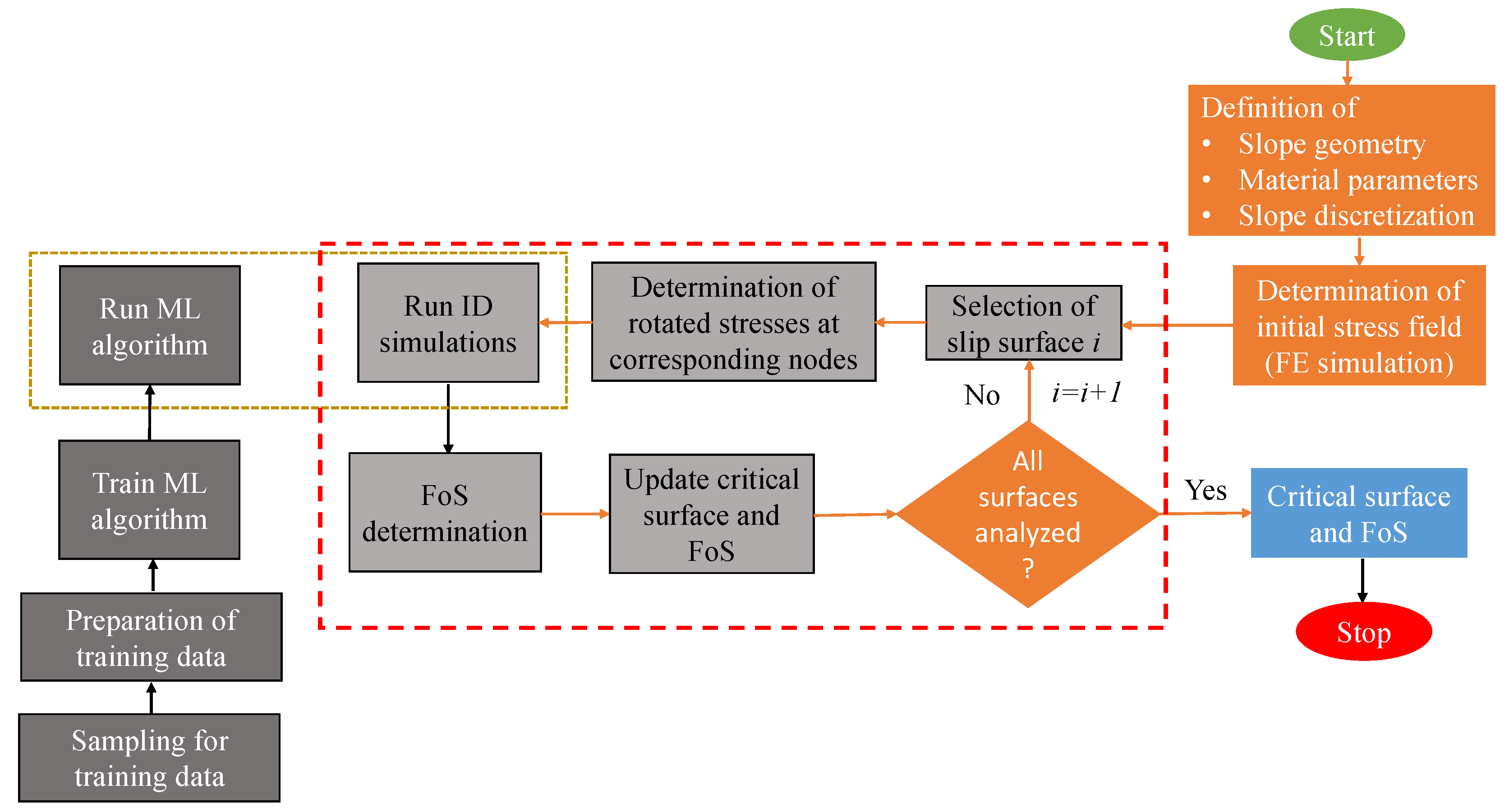
2.3. Application of Machine Learning in SDSS

To detect the critical slip surface, SDSS requires the evaluation of element tests at multiple points along potential slip surfaces. Furthermore, searching for the critical slip surface entails evaluating element tests along multiple potential slip surfaces, each with multiple points along the slip surface. Depending on the implemented optimization scheme (e.g., brute optimization, differential evolution [40], particle swarm optimization [41], genetic algorithms [42]), and desired accuracy, more than 10,000 element test simulations may be required for identifying the critical slip surface [33]. Additionally, in case of boundary value problems considering temporal effects, for instance slopes subjected to seismic loading, multiple time steps need to be analyzed, resulting in huge computational cost. Machine learning (ML) algorithms can help reducing the computational costs associated with SDSS significantly by substitution of the computing-intensive Incremental Driver simulations with ML algorithms, as summarized in the flowchart in Figure 3. To replace element test simulations conducted with Incremental Driver by ML, an ML algorithm needs to be selected, data for training and testing needs to be sampled and the ML algorithm needs to be trained first.

Previous studies [33] and additional investigations revealed that many different ML algorithms, for instance radial basis functions (RBF), K-nearest neighbors (KNN), random forest (RF), multilayer perceptron (MLP), or support vector machines (SVM), could be used to enhance SDSS by ML. Although MLP did not provide the most accurate predictions in the aforementioned study, it was selected in this study to emphasize the importance of the sampling approach. The multi-layer perceptron (MLP) model is applied from the scikit-learn package. Note that the settings of the MLP algorithms used within the framework of SDSS are reported in Section 3.3.

After selection of an adequate ML algorithm, sampling is necessary to generate data required for training and testing of the ML algorithm. As ML is used here to approximate the stress–strain behavior for a specific loading path (i.e., DSS test) considering a fixed constitutive model with constant material parameters, the results are only dependent on the initial conditions, which include the initial stress tensor and the initial values of the state variables. As plane strain conditions apply for DSS tests, only four components of the stress tensor need to be considered. Five additional dimensions could be added by consideration of the state variables of the hypoplastic model. Those include the void ratio and four components of the intergranular strain (IGS) tensor in case this extension of hypoplasticity [43] is used. As the consideration of IGS leads to increased stiffness at small strains, shear stresses as well as $T\left(\gamma \right)$ may be over-predicted, leading to non-conservative estimates of the FoS [33]. For this reason, the IGS extension is not used in the current study. The basic hypoplastic model [36] is applied. Consequently, five input variables (i.e., dimensions) are considered for the sampling and training of the ML algorithms: four stress components (three normal stresses ${\sigma }_{xx},{\sigma }_{yy},{\sigma }_{zz}$ and one shear stress ${\tau }_{xy}$) and one state variable (void ratio e). Note that these five variables are not fully independent as constraints, such as limit surfaces or limit void ratios need to be considered. Further details regarding those constraints are discussed in the following section.

3. Sampling

3.1. Motivation

To train a machine learning algorithm for a specific problem, a proper sampling strategy is needed to ensure that sample points are well distributed inside the input parameter space. Equally essential is the definition of suitable ranges of variables and relevant constraints. As the training and potentially also the evaluation of ML algorithms is dependent on the training sample size, the objective is to use the least number of samples that guarantees a proper distribution within the n-dimensional space. In this regard, the type of sampling method has a major impact on the sampling output and, thus, on the training quality and the ML algorithms’ predicted output. Among others, common sampling approaches include grid, stratified, cluster, weighted, Monte Carlo, and Latin hypercube sampling (LHS). Out of those, six sampling approaches are described in more detail and applied throughout this study. The interested reader can find more detailed information about sampling techniques in specialized references like, for example, [44,45,46].

Grid sampling, otherwise also known as uniform sampling, uses a certain fixed spacing between the input parameter values. The sample parameter values in each input dimension are combined with each other so as to form a grid of samples. The major drawback of grid sampling is that it only samples specific grid values, leaving empty spaces in all dimensions of the input parameter space. Therefore, the use of uniform sampled data for training ML algorithms cannot always ensure proper output prediction throughout the space, and the quality of predictions depends on the density of the sampling grid. To ensure a larger number of samples for lower stresses, grid spacing can be modified, for instance, by accounting for quadratic spacing between the input parameters. An alternative method that uses random sampling is based on the Monte Carlo technique [47]. This method generates N samples in a sample space S. The method, though simple, does not ensure proper distribution between samples in the input parameter space, and the user has very little control over the final sample distribution. A better random sampling strategy could be applied using Latin hypercube sampling (LHS) [48]. This is a stratified sampling procedure where each component K of sample space S is partitioned into N intervals. Each interval is assigned a probability of $1/N$, thus leading to the sample partitioning into $N_k$ samples. The LHS sample of size N is thus obtained by assigning one random observation in each cell.

For many applications, the sampling approaches discussed above must also consider constraints to avoid generating sample points with combinations of input parameters that violate well-established soil mechanical conditions. Samples not violating the constraints are considered valid samples. Among others, those constraints can be formulated based on stresses to account for limiting surfaces or based on limiting void ratios at given mean pressures [49]. Suitable limiting surfaces for soils can be defined based on various surface shapes in the principal stress space, for instance, cylinders (von Mises), cones (Drucker–Prager), cones with hexagonal base (Mohr–Coulomb), cones with hexagonal base and rounded corners (e.g., Matsuoka–Nakai, Lade–Duncan) or ellipsoids (Modified CamClay). In this study, the Matsuoka and Nakai [50] criterion depending on the stress invariants $I_1$, $I_2$ and $I_3$ and the friction angle $\phi$ (Equation (2)) is applied as constraint since the same function is incorporated as limiting surface in the hypoplastic model.

$$\frac{I_1{I}_2}{I_3}=8{tan}^2\phi +9=\frac{9-{sin}^2\phi }{1-{sin}^2\phi }=K_{\mathrm{MN}}$$

(2)

In the simulation of element tests using hypoplasticity, it is fundamental to ensure that void ratios do not evolve beyond the limit void ratio $e_i$ (loosest state) or below $e_d$ (densest state), respectively, for a given mean effective stress p. Those limit void ratios constitute an additional constraint for the sampling process and the randomly generated values of void ratios must be validated against the limits imposed by Bauer’s law [49] as summarized in Equation (3), where $e_{i0}$, $e_{c0}$, $e_{d0}$ denote the respective void ratios at the loosest, critical, and densest state at zero mean effective stress, $h_s$ is the granular hardness, n is a material constant and $\mathbf{\sigma }$ is the stress tensor. Note that in this study, the void ratios at densest state $e_d$ and at critical state $e_c$ are considered as respective lower and upper limits during sampling.

$$\frac{e_i}{e_{i0}}=\frac{e_c}{e_{c0}}=\frac{e_d}{e_{d0}}=exp\left[-{\left(\frac{-\mathrm{tr}\mathbf{\sigma }}{h_s}\right)}^n\right]$$

(3)

Imposing constraints to the sampling process can significantly reduce the amount of valid samples needed to train the ML algorithms (A sufficient number of samples has to be generated to populate the n-dimensional sampling space considering problem-specific constraints. In general, the process to determine the number of samples is based on trial and error, considering a desired level of accuracy in the predictions). Let us consider 60,000 samples generated using Latin hypercube sampling (LHS) as shown in the top row of Figure 4. When the constraints summarized in Equations (2) and (3) are implemented, a significant reduction of samples is observed as shown in the bottom row of the same figure. Although only four out of ten projections are shown here, the influence of the constraints can clearly be seen. A significant number of rejected samples corresponds to lower stress states (e.g., ${\sigma }_x\le 100$ kPa). Violation of the constraints is more likely for lower stresses due to smaller ranges of admissible stress states. In contrast, significantly more amounts of samples at higher stress levels (e.g., ${\sigma }_x\ge 200$ kPa) fulfilled the constraints and, thus, were not removed. In total, consideration of the constraints led to a reduction of the number of samples from 60,000 to approximately 10,000. Although not explicitly depicted here, this issue does not solely apply to LHS, as emphasized in Figure 4, but is also observed for grid sampling with linear or quadratic spacing, Monte Carlo sampling or other standard sampling techniques identical constraints. To ensure that ML algorithms are trained with the intended number of samples—in this case 60,000—that also should not violate the aforementioned constraints, larger initial sample sizes need to be defined. However, following this strategy, the sample distribution will be unsatisfactory as the number of samples accepted for small stresses would still be small compared to those accepted for larger stresses, resulting in an inhomogeneous distribution of samples along the desired stress range. This is also depicted in Figure 5 showing four out of ten projections for approx. 60,000 valid samples that were generated using grid sampling with linear and quadratic spacing (1st and 2nd row), Monte Carlo sampling (3rd row), and Latin hypercube sampling (4th row).

Grid sampling with quadratic spacing was used in [33] to train different ML approaches within the concept of SDSS, where similar issues regarding the distribution of samples at lower stresses were also reported. The ML algorithms over-predicted ${\tau }_{xy}-\gamma$ curves at low mean effective stresses compared to Incremental Driver simulations. The over-prediction eventually resulted in an overestimation of the factor of safety (FoS) obtained using SDSS. The over-prediction of the FoS results in an unsafe design must be avoided under any circumstances. Considering the above discussions, modification of sampling approaches is required to enable more accurate predictions of the shear stress vs. shear strain behavior (e.g., for simple shear tests). For this reason, two modified sampling algorithms are presented in the following section. The approaches referred to as “Modified Latin Hypercube sampling 1 (LHS-1) and 2 (LHS-2)” are based on sampling and resampling using Latin hypercube sampling and allow for more accurate predictions of the shear stress vs. shear strain behavior, especially for small stress states.

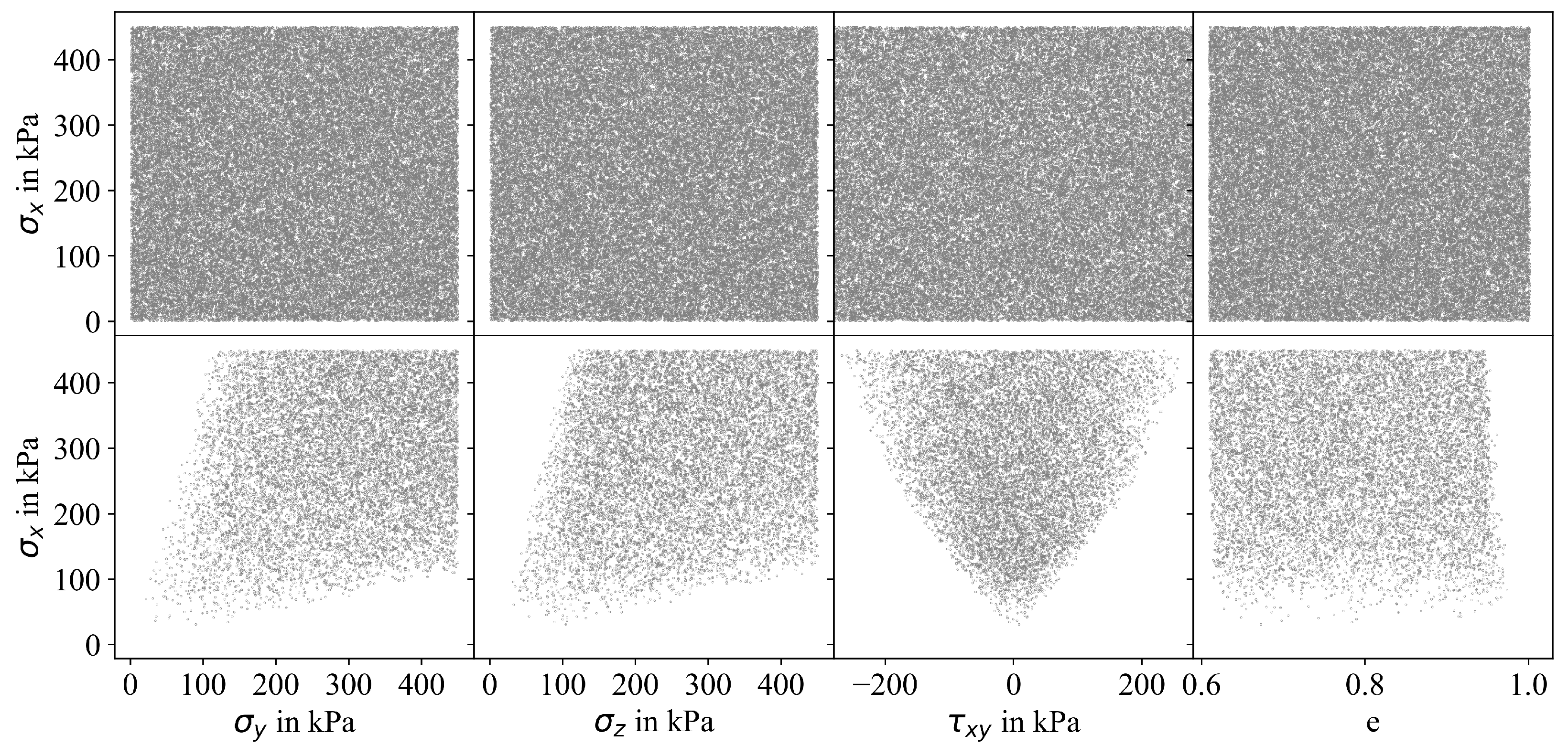
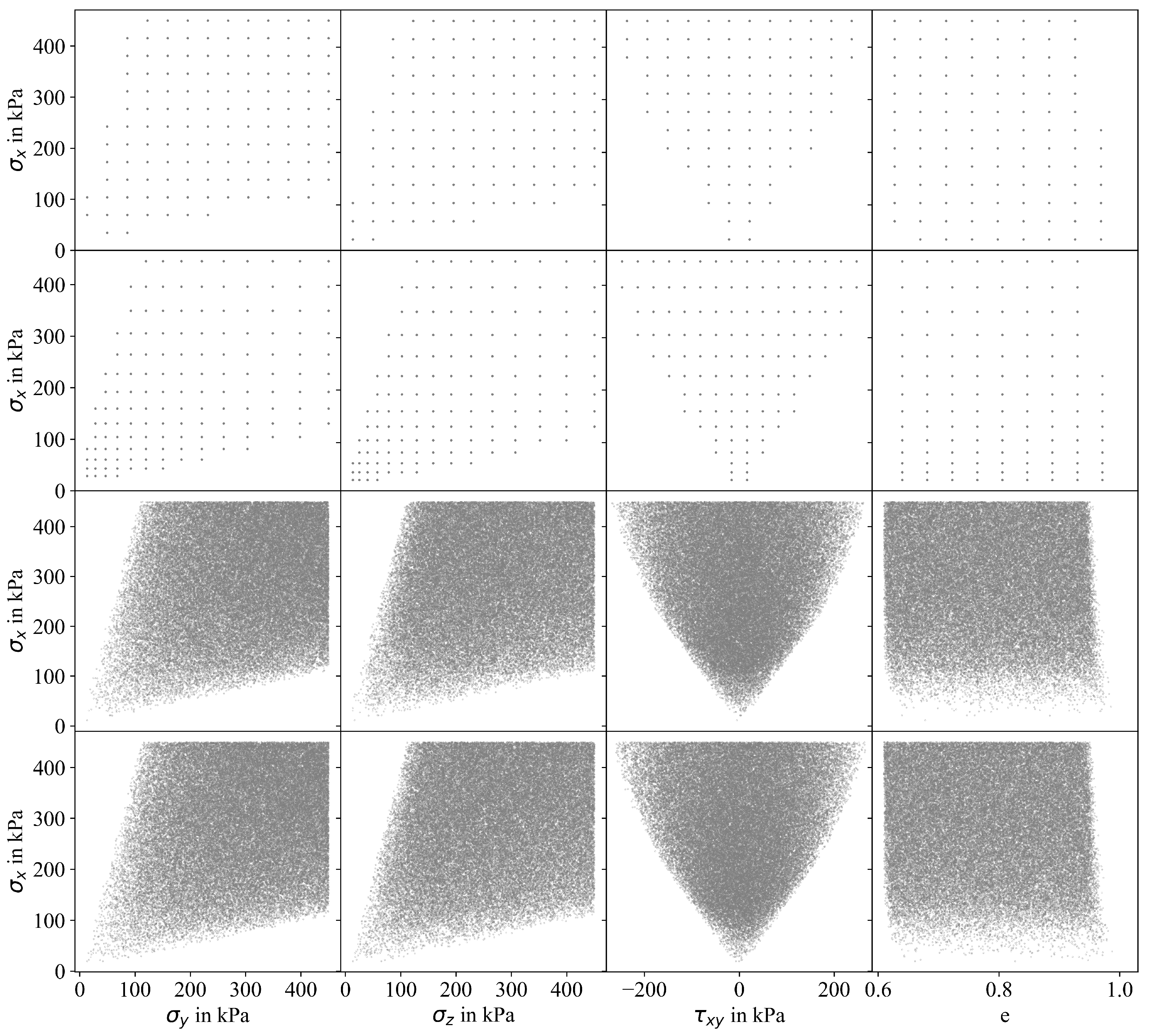
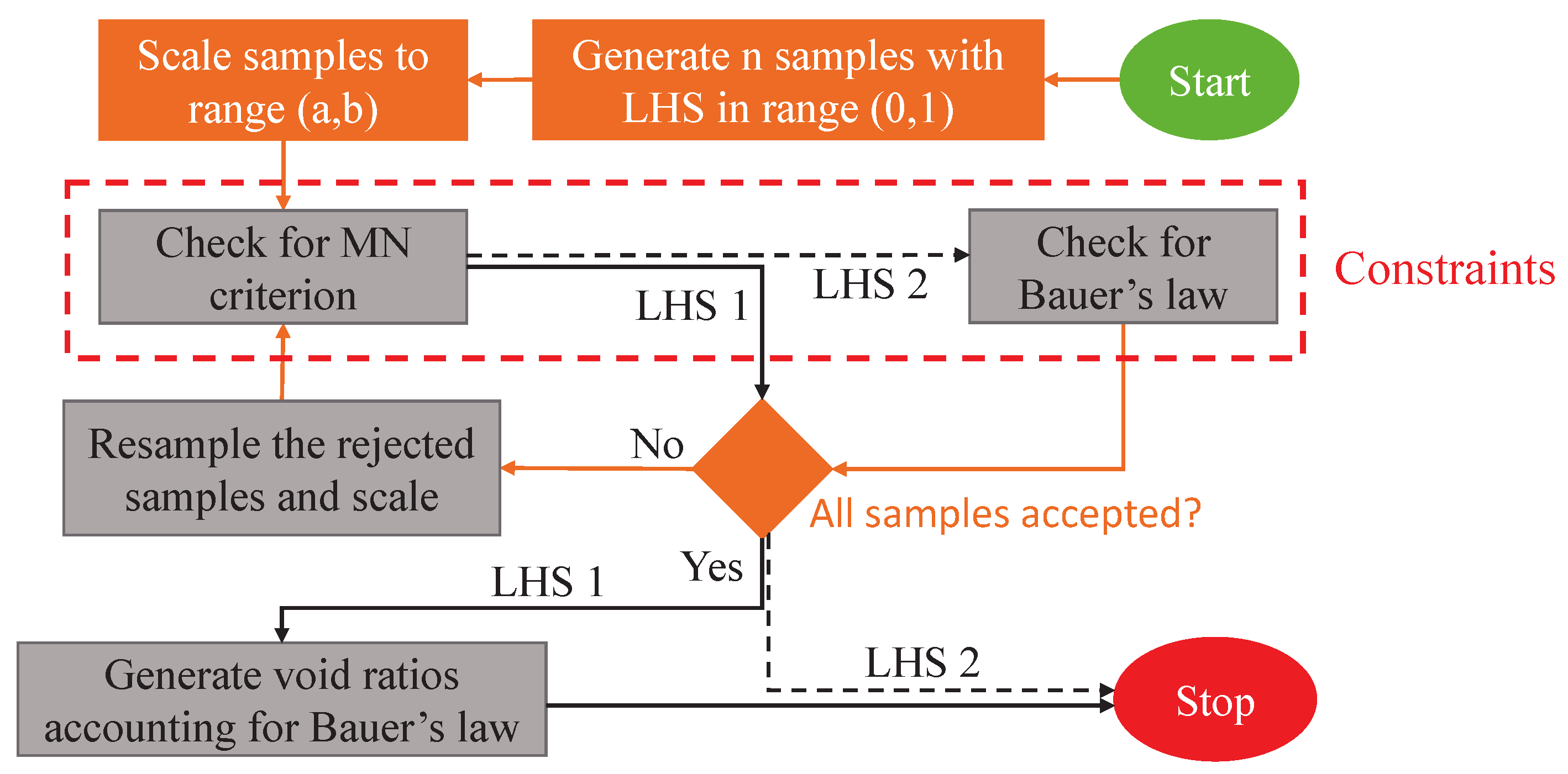
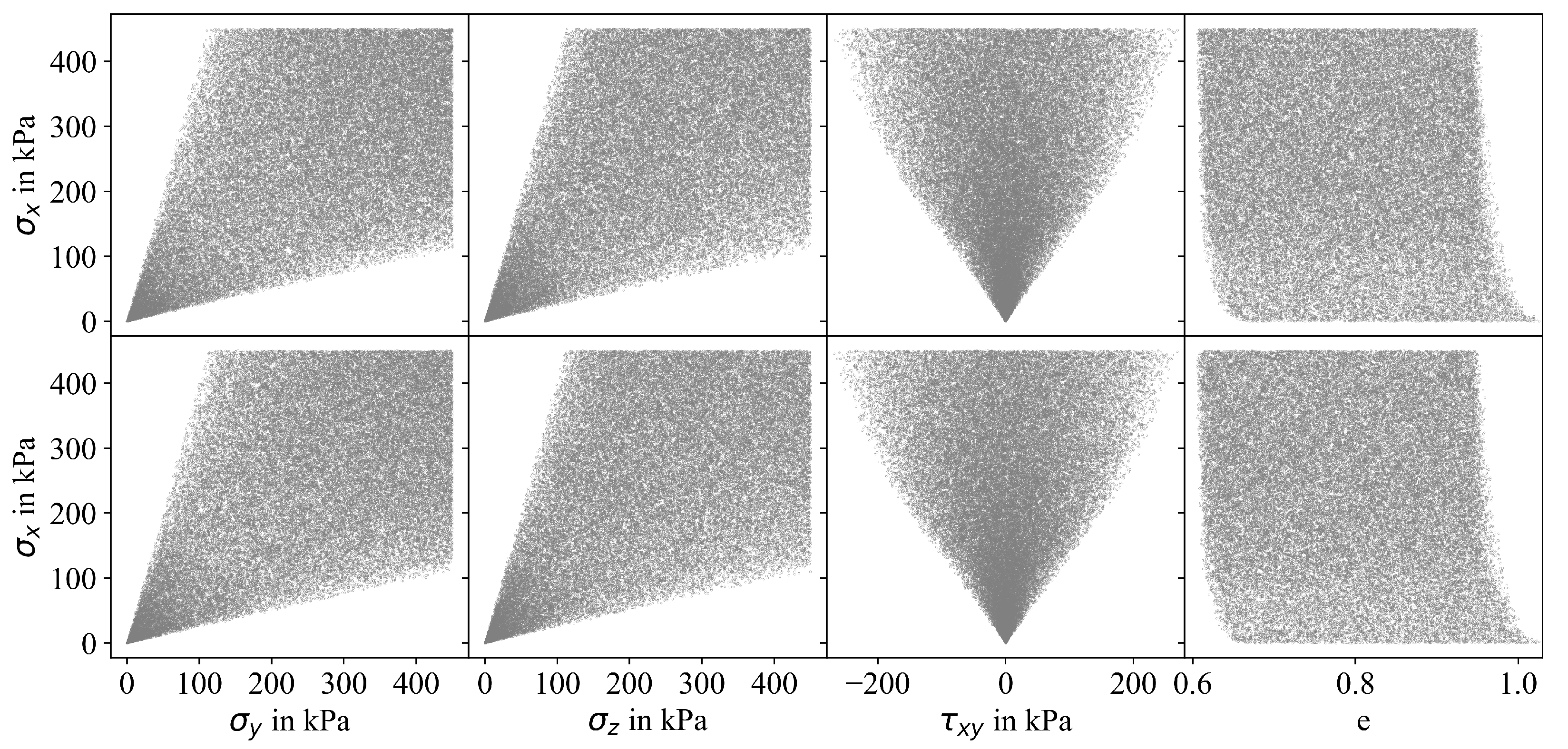
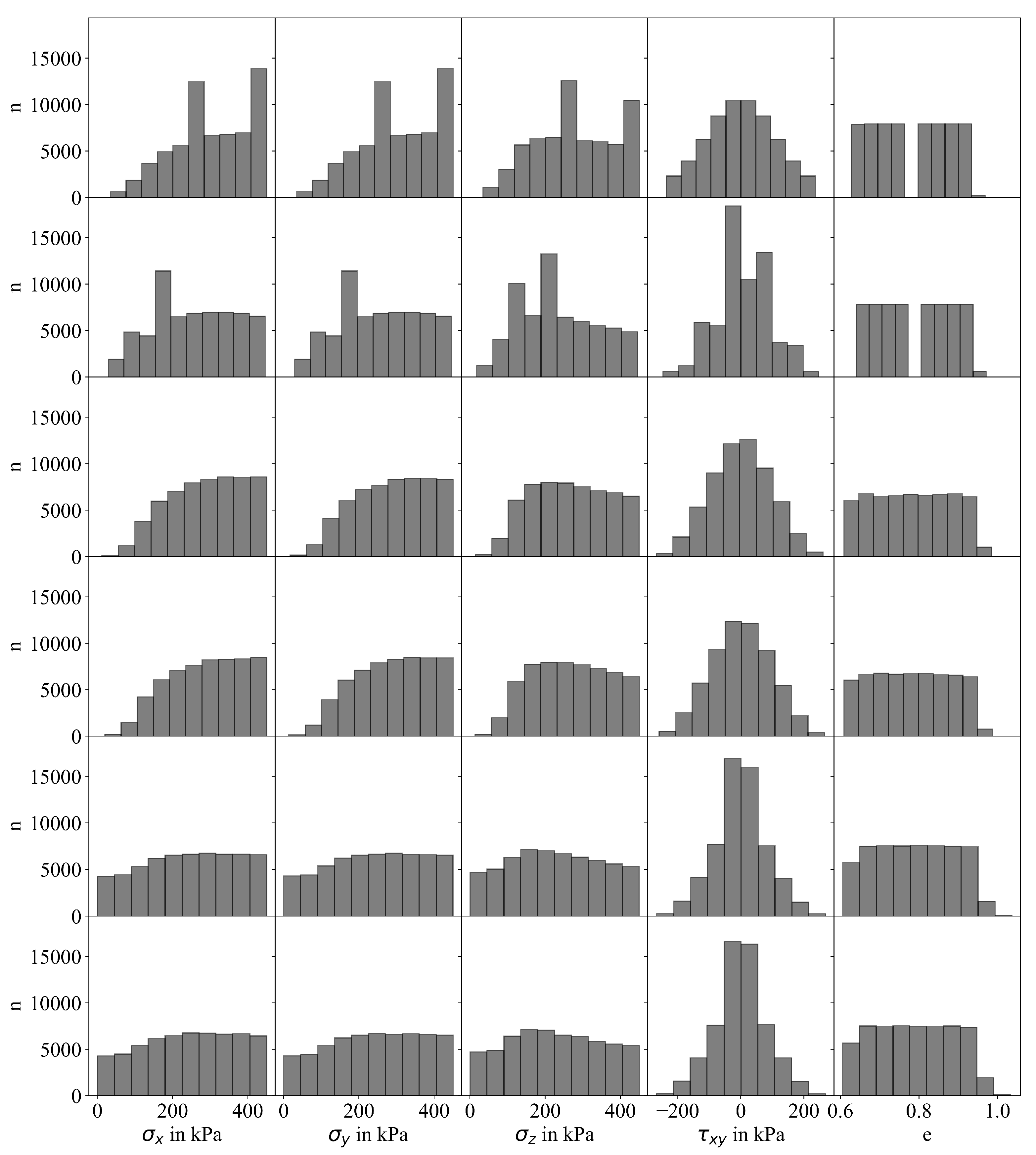
3.2. Modified Sampling Approaches

As discussed in Section 3.1, many sampling algorithms yield proper distributions of samples for cases without constraints. However, as sampling for application in SDSS involves constraints limiting potential unfeasible combinations of stress states and void ratios, many samples generated using those sampling algorithms were eliminated as shown for the case of LHS in Figure 4. The desired number of valid samples was achieved by increasing the initial sampling size, as shown in Figure 5. However, this resulted in an uneven distribution of samples across the entire stress range. Using those distributions of samples for training an ML algorithm would lead to an inaccurate approximation of shear stress vs. shear strain curves, especially for lower stress levels. One of the main reasons for this issue was that smaller stress levels had a higher probability of violating the constraints compared to larger stress levels. This was due to the narrower admissible ranges in the input dimensions for smaller stress levels.

To improve the quality of the sampling, two modified Latin hypercube sampling approaches (LHS-1 and LHS-2) are formulated and schematically presented in Figure 6. Both approaches start with a Latin hypercube sampling with the desired number of samples considering five independent dimensions (${\sigma }_x$, ${\sigma }_y$, ${\sigma }_z$, ${\tau }_{xy}$, and e). After the generation of samples using LHS within the ranges of 0 and 1, samples are scaled to the desired lower and upper bounds of the respective dimensions. Afterwards, an iterative procedure for both approaches is applied, whereby the workflow of the two algorithms differs slightly. In LHS-1, the constraint limiting unfeasible stress states, for instance violating the Matsuoka–Nakai criterion (Equation (2)), is checked, while in LHS-2, two constraints, the Matsuoka–Nakai criterion (Equation (2)) and Bauer’s law (Equation (3)) are checked. If there are any samples that do not meet the specified constraint(s), they will be resampled. To ensure an adequate number of samples generated at small stress levels, the first stress component (${\sigma }_x$) is kept constant during resampling, while the other stress components (${\sigma }_y$, ${\sigma }_z$ and ${\tau }_{xy}$) and the void ratio e (only for LHS-2) are resampled using the conventional LHS. This iterative procedure is repeated until all samples fulfill the constraint(s). Based on trial analyses, approximately 1/3 of the initial samples are accepted directly, while additional 30–35 iterations are required for the remaining samples. Note that the overall sampling process including resampling iterations takes less than onew minute. Once all samples comply with the constraint(s), the iteration procedure stops. At the end of the iteration process, LHS-2 approach is finished, while an additional step is required for LHS-1. Sampling and scaling of the fifth dimension (i.e., void ratio) is performed using 1D Latin hypercube sampling considering the individual limiting void ratios in accordance with Bauer’s law (Equation (3)).

Four projections (${\sigma }_x$ vs. ${\sigma }_y$, ${\sigma }_x$ vs. ${\sigma }_z$, ${\sigma }_x$ vs. ${\tau }_{xy}$ and ${\sigma }_x$ vs. e) of the five-dimensional space are depicted in Figure 7 for LHS-1 (top row) and LHS-2 (bottom row). It can be seen from those projections that both modified Latin hypercube sampling approaches improved the distribution of samples significantly, allowing for a higher number of samples in the lower stress range compared to the standard sampling algorithms. Note that although an increased number of samples is located at lower stresses after resampling, the generated samples still cover the full domain properly.

The quality of the distribution of samples following the stress and void ratio constraints for different sampling methods can be summarized by plotting the frequency distribution of each set of generated variables in terms of histograms. The scarcity of samples in a specific stress range is reflected in an inhomogeneous distribution of the corresponding histogram. An improved sampling strategy that guarantees better coverage of the entire sampling space should produce quasi-uniform and symmetric histograms. In Figure 8 the frequency distributions of the four stress components and void ratio generated with grid sampling with linear spacing, grid sampling with quadratic spacing, Monte Carlo, Latin hypercube sampling, and modified LHS-1 and LHS-2 are presented. Grid sampling with linear and quadratic spacing (Figure 8-rows 1,2) produced multimodal skewed left distributions for the normal stresses and bimodal distributions for the void ratio with a gap around $e\approx 0.8$. Monte Carlo and Latin hypercube sampling (Figure 8-rows 3,4) resulted in unimodal skewed left distributions for normal stresses. The skewed left distributions evidence the problem that conventional sampling methods suffered in producing enough samples for lower stresses that fulfilled all constraints. In contrast, the modified LHS-1 and LHS-2 showed a more uniform distribution of normal stresses for all ranges of interest. Histograms for ${\tau }_{xy}$ exhibit a symmetric unimodal distribution that could be described with a Gaussian distribution function. The high concentration of samples around ${\tau }_{xy}=0$ coincides with the needed increase in non-rejected normal stress samples near the low stresses range after resampling.

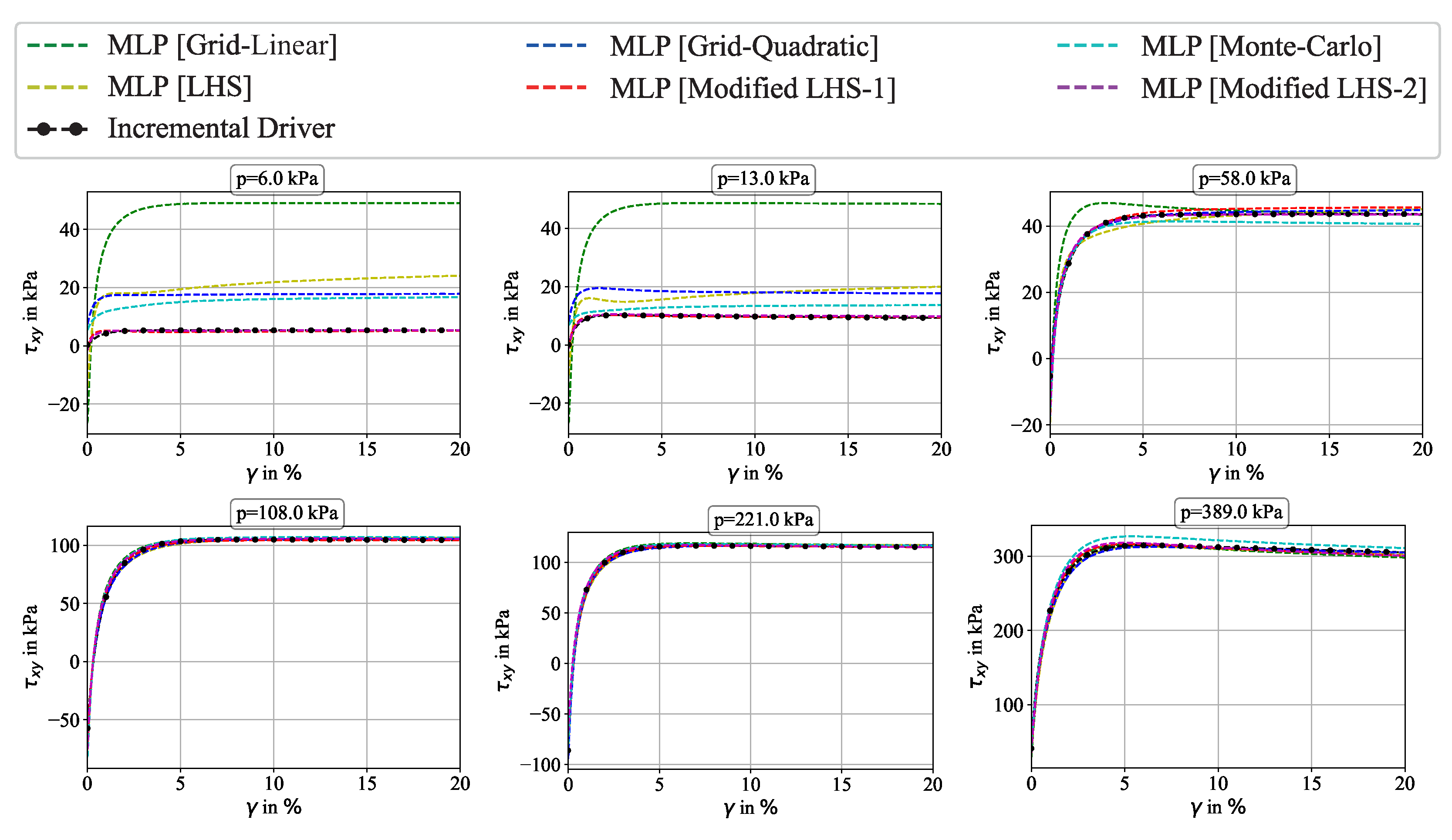
3.3. Influence of Sampling Approach on Accuracy of MLP Prediction

This study investigates the impact of the sampling approach on the accuracy of the ML prediction compared to the simulation of direct simple shear (DSS) element tests using hypoplasticity in Incremental Driver (ID). The sampling approaches under investigation considered the Matsuoka–Nakai and Bauer’s law constraints and included grid sampling with linear/uniform and quadratic spacing, Monte Carlo sampling, Latin hypercube sampling and both modified Latin hypercube sampling approaches (LHS-1 and LHS-2) presented in Section 3.2. For all sampling approaches under investigation, MLP with three hidden layers, each composed of 290 neurons, and a “logistic sigmoid” activation function was used. These MLP settings were chosen based on trial analyses. The training was conducted considering 60,000 valid samples accounting for the aforementioned constraints. In the case of the four traditional sampling approaches, larger initial sample sizes were needed (see Figure 5), whereas in the modified Latin hypercube sampling approaches, samples violating constraints were resampled following the concept of LHS-1 or LHS-2 presented in Section 3.2 with the final distribution of samples depicted in Figure 7. The influence of sampling strategies was validated using new sampling points. A total of 3000 new test samples were generated, 1500 each with LHS-1 and LHS-2. Shear stress vs. shear strain curves were produced with MLP using the validation samples. Simulations of DSS element tests with ID were conducted using the stress states and void ratios generated in the validation set as initial conditions.

Representative results of shear stress vs. shear strain curves for test samples with different initial mean effective stresses are depicted in Figure 9. The curves were obtained from MLP predictions and DSS simulations with ID and hypoplasticity using the validation set. It is apparent from this figure that good agreement between MLP using all sampling approaches and the element test simulations with the hypoplastic model was obtained for large mean stresses ($p\ge 100$ kPa), while minor differences were obtained for intermediate mean stresses ($p=58$ kPa). Note that for the latter case, the accuracy of the predicted shear stress vs. shear strain curve decreased using grid sampling with linear spacing due to over-prediction of shear stresses for shear strain levels $\gamma \le 10\%$. Significant differences between the curves predicted by MLP and ID were obtained for smaller mean stresses ($p=6$ kPa and $p=13$ kPa). In the case of grid sampling with linear spacing and traditional LHS, large initial offsets in the predicted shear stresses were seen. All four traditional sampling approaches significantly overestimated the shear stresses for the whole range of shear strains applied. In contrast, it was observed that the predictions of the MLP model using the modified Latin hypercube sampling approaches LHS-1 and LHS-2 resulted in good agreement with the ID results for all stress ranges.

The accuracy of the predictions of the MLP model using different sampling approaches for the 3000 test samples was evaluated in terms of the coefficient of determination limited to $0.0\le R^2\le 1.0$. Overall, a good approximation of the shear stress response from ID was obtained with MLP in combination with all sampling approaches, as indicated by coefficients of determination varying in the range $0.773\le R^2\le 0.913$ (see

Table 1. Accuracy of MLP in terms of $R^2$ using different sampling approaches.

	$\mathit{p}\le 20\mathbf{kPa}$	$20\mathbf{kPa}\le \mathit{p}\le 100\mathbf{kPa}$	$\mathit{p}\ge 100\mathbf{kPa}$	Overall
Grid sampling with linear spacing	0.000	0.313	0.858	0.773
Grid sampling with quadratic spacing	0.000	0.750	0.934	0.887
Monte Carlo sampling	0.011	0.642	0.938	0.879
Latin hypercube sampling	0.003	0.603	0.878	0.823
Modified Latin hypercube sampling-1	0.328	0.856	0.936	0.913
Modified Latin hypercube sampling-2	0.769	0.823	0.917	0.907

). However, the evaluation of $R^2$ regarding different mean stress ranges revealed that the MLP predictions utilizing different sampling approaches varied strongly. The best agreement between ID and MLP was obtained for large mean stress levels ($p\ge 100$ kPa) for all sampling approaches ($0.858\le R^2\le 0.938$). A lower level of agreement was observed for intermediate mean stress levels (20 kPa $\le p\le 100$ kPa). In that range, the lowest $R^2$ was obtained using grid sampling with linear/uniform spacing ($R^2=0.313$), while the other sampling approaches resulted in $0.603\le R^2\le 0.856$. As expected, no improvement of $R^2$ was seen using the modified Latin hypercube sampling approaches LHS-1 and LHS-2 for large mean stress levels. This can be explained by the smaller number of samples for large mean stress levels. However, as the difference in $R^2$ was small, the predictions of MLP using LHS-1 and LHS-2 for large mean stress levels could be considered accurate. In the case of intermediate mean stress levels, it was observed that the LHS-1 and LHS-2 approaches provided better estimates compared to the other sampling approaches as a result of higher sample densities that could also be seen by comparing the distribution of samples depicted in Figure 5 and Figure 7.

As intended, the most pronounced differences between the $R^2$ values obtained with the six sampling approaches were seen for smaller mean stress levels. In contrast to the traditional approaches providing very small coefficients of determination ($0.0\le R^2\le 0.011$), indicating very low accuracy of the shear stress vs. shear strain behavior obtained in a DSS test, the modified Latin hypercube sampling approaches (LHS-1 and LHS-2) resulted in significantly improved approximations. It is worth noting that there is a significant difference in the results obtained when using MLP in combination with the modified Latin Hypercube sampling methods LHS-1 and LHS-2, with the latter performing better than the former. These differences can be directly related to the different sampling strategies employed, particularly when dealing with the void ratio. In LHS-1, the void ratio is sampled using LHS. However, apart from considering individual bounds in accordance with Bauer’s law, this is done separately from the four stress components. It is possible that small stresses were only combined with void ratios associated with large relative densities, as it is not checked whether LHS-1 results in a proper distribution of samples in the 5D space. This deficit was overcome in LHS-2 by incorporating the void ratio in the resampling process, which allowed Latin hypercube sampling to consider four variables instead of three, with the void ratio sampled separately.

4. Influence of Sampling on the FoS for Slopes Subjected to Different Loading

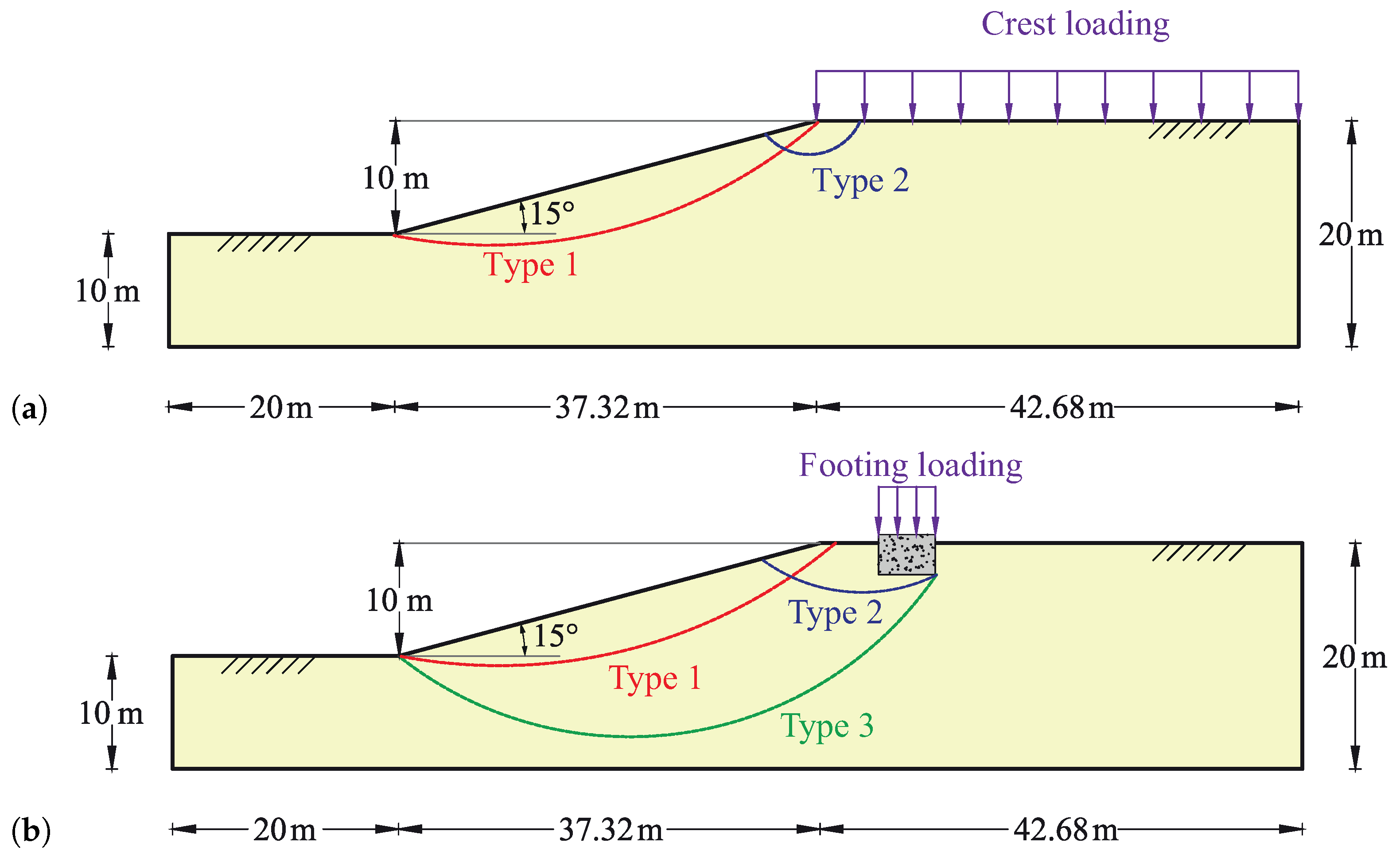
4.1. Methodology

The selection of the sampling approach has a decisive influence on the accuracy of the stress–strain behavior predicted by the machine learning algorithm, especially for small mean stresses, as extensively discussed in Section 3 with the simulation of element tests. Now, the effect of sampling techniques is studied on the scale of geotechnical boundary value problems, where the stability of a slope with an inclination of 15° subjected to two different loading conditions was analyzed in terms of the factor of safety (FoS) using the concept of strain-dependent slope stability (SDSS) proposed by [34] and outlined in Section 2.1. In the first example depicted in Figure 10a, the slope is subjected to an external uniform distributed load applied on the crest, whereas in the second example presented in Figure 10b, an embedded foundation at the crest is considered. In both examples, the soil is considered dry with an initial relative density of $D_R=40\%$. The material behavior of the soil is described using the hypoplastic constitutive model [36], which requires the definition of the following material parameters: the critical friction angle ${\phi }_c$, the void ratios (at zero mean effective stress) at densest state $e_{d0}$, at critical state $e_{c0}$ and the maximum void ratio in a suspension $e_{i0}$, the granular hardness $h_s$, and the exponents n, $\alpha$ and $\beta$. The parameter set utilized in this study is shown in

Table 2. Parameters of the hypoplastic model for the slope material.

${\mathit{\phi }}_{\mathit{c}}$ in °	hs in MPa	n	${\mathit{e}}_{\mathit{d}0}$	${\mathit{e}}_{\mathit{c}0}$	${\mathit{e}}_{\mathit{i}0}$	$\mathit{\alpha }$	$\mathit{\beta }$
33.1	4000	0.27	0.677	1.054	1.212	0.14	2.5

. The finite element simulations were carried out using the software numgeo ([51,52,53,54] and www.numgeo.de, accessed on 21 December 2023). The simulations were performed in the following steps: first, in the geostatic step, gravitational load (soil weight) was considered and an additional artificial load of 0.1 kPa acting perpendicular to the top surface was applied for the purpose of numerical stability. Secondly, loads q acting at the crest of the slope and on the embedded foundation were increased incrementally up to 200 kPa (example 1) and 600 kPa (example 2). Lastly, the factor of safety of the slopes was quantified based on the SDSS method.

Considering the spatial distribution of stresses and state variables (e.g., void ratio) obtained from numgeo at different loads, stability analyses were conducted using SDSS, quantifying the factor of safety in terms of ${\mathrm{FoS}}_{max}$. SDSS was conducted with shear stresses determined in accordance with direct simple shear (DSS) tests performed at each node. The element test simulations for the DSS tests were carried out using Incremental Driver (ID). Although SDSS could be implemented for different shapes of slip surfaces (e.g., planar, circular, or polyline), only circular slip surfaces with 20 nodes are considered in the current study. As the location of the critical slip surface is unknown a priori, many slip surfaces need to be investigated. In accordance with the discussions by Schmüdderich et al. [33], differential evolution [40] was used as an optimization algorithm to determine the critical slip surface.

Stability analyses were conducted at predefined load intervals of $\Delta q=20$ kPa (example 1) and $\Delta q=100$ kPa (example 2) to investigate the influence of the magnitude of loading on the FoS. To study the influence of the sampling approach on the FoS prediction, comparative analyses with multi-layer perceptron (MLP) trained based on different sampling approaches were undertaken, considering the results obtained with ID as the proper solution. In accordance with Section 3.3, four traditional sampling approaches (grid sampling with linear and quadratic spacing, Monte Carlo sampling, and Latin hypercube sampling) and both modified Latin hypercube sampling approaches (LHS-1 and LHS-2) were considered for the FoS estimation of both slopes. Although grid sampling with linear spacing provided inaccurate approximations of the shear stress for small mean stress levels (see Section 3.3), it was included in this section to allow for a comprehensive comparison of the FoS predictions.

In addition to the FoS, the shape of the critical slip surfaces associated to the smallest FoS was investigated. Note that for the first example, very shallow slip surfaces were mostly expected (failure types 1 and 2 in Figure 10a) since the friction angle governs the shear strength and the surcharge is acting on the top surface. For the second example, shallow (failure type 1 in Figure 10b) and deep (failure types 2 and 3 in Figure 10b) slip surfaces are expected depending on the magnitude of load applied to the embedded foundation. For small magnitudes, shallow slip surfaces might be observed that do not interfere with the foundation, while for increased loads slip surfaces might start right below the foundation. Thus, there should be a threshold load separating different types of slip surfaces. Note that discussions with regard to different types of slip surfaces depending on load magnitudes or interfering objects in close proximity were also provided in previous studies with regard to the bearing capacity problem [55,56].

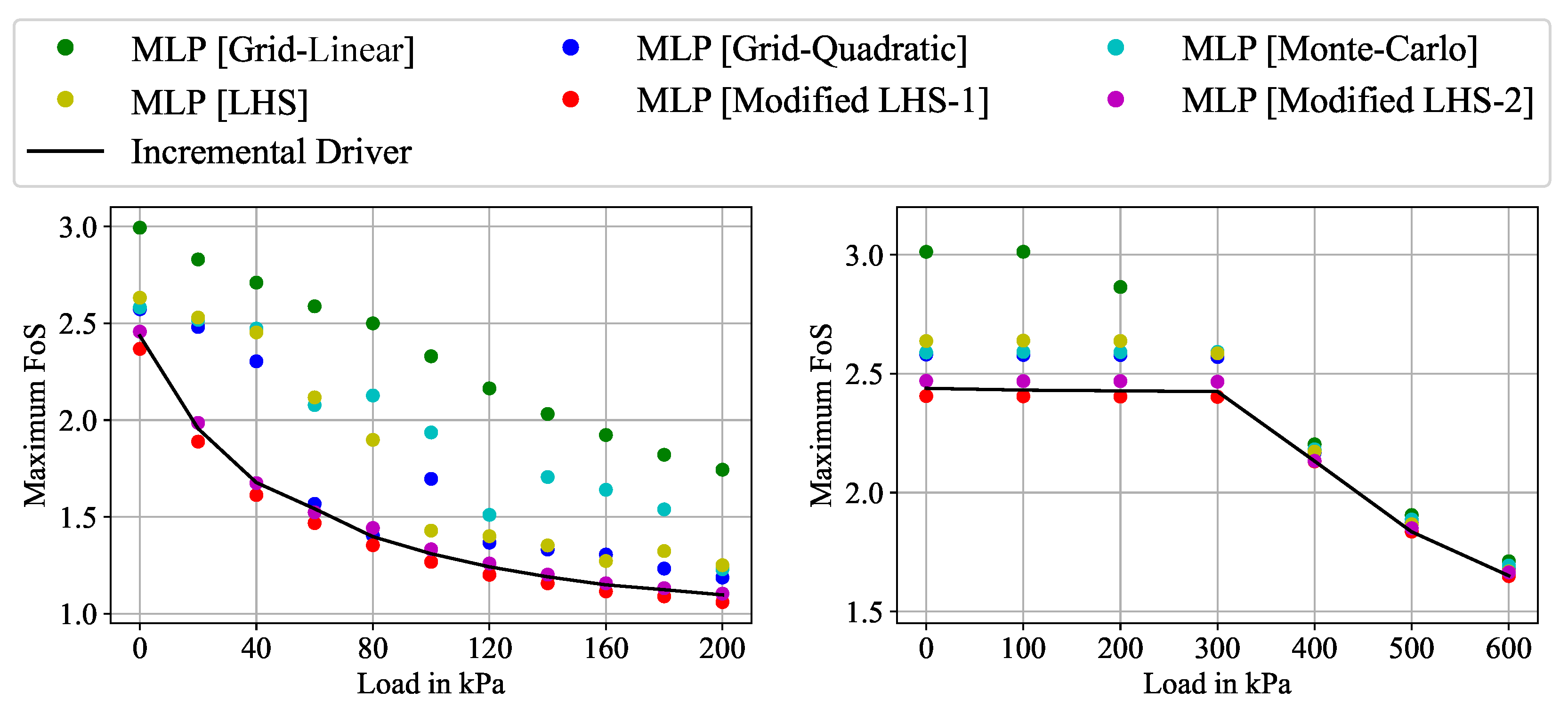
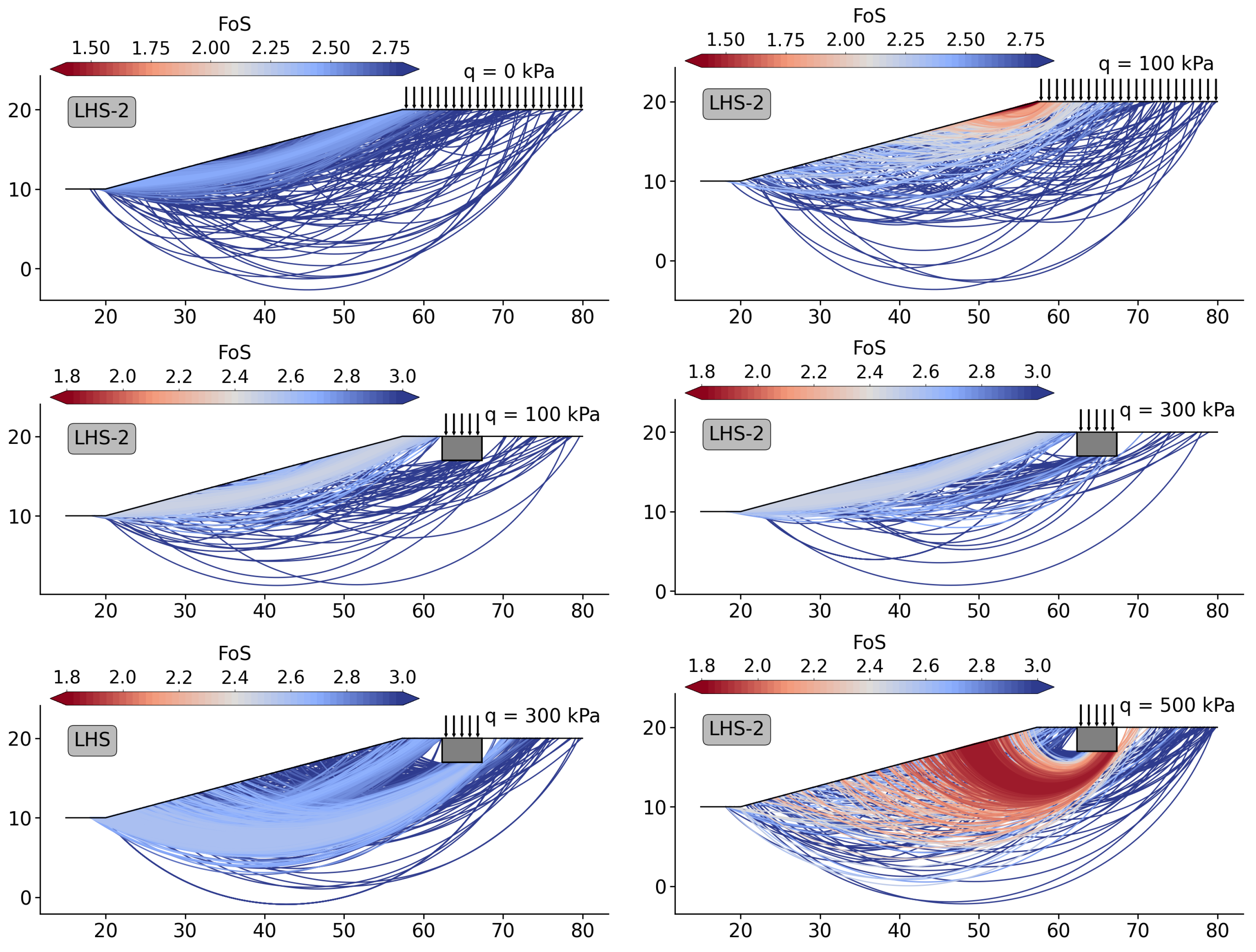
4.2. Results and Discussion

Figure 11 depicts the results in terms of the factors of safety (FoS_max) versus applied vertical loads based on SDSS analyses obtained with ID and MLP using different sampling approaches for both slope examples. As mentioned in Section 2.1, the SDSS analysis can yield two FoS depending on whether the global mobilized shear resistance ratio T reaches a peak value and then decreases. All the results presented and discussed in this section refer to the peak FoS, also denoted as FoS_max. Figure 11-left presents the results of example 1 (Figure 10a), where a uniform load is acting on the crest of the slope. Analyzing the results obtained with ID (continuous line), that the initial level of safety ($\mathrm{FoS}=2.44$) obtained with SDSS for the case of zero surcharge is in good agreement with the rough estimate of $tan{\phi }_c/tan\beta =2.43$, with $\beta ={15}^{\circ }$ being the slope inclination. Moreover, FoS decreases with increasing surcharge applied on the slope crest until the stability approaches $\mathrm{FoS}=1.0$ for a surcharge of 200 kPa. Note that convergence of the FE simulations could not be obtained for loads exceeding 200 kPa, which is in good agreement with the FoS falling below the value of 1.0. Based on the evaluation of slope stability using MLP with different sampling methods, it can be observed that there is a strong agreement between MLP and ID for LHS-1 (red points) and LHS-2 (purple points). However, the other four traditional approaches (grid sampling with linear and quadratic spacing, Monte Carlo sampling, and Latin hypercube sampling) exhibit a wider range of variation in the factor of safety (FoS). Overall, grid sampling with linear spacing led to the largest FoS for all loads investigated, while the other traditional sampling approaches showed oscillating deviations. It is also worth noting that the variation of FoS with the increasing vertical load follows an almost linear pattern for the grid sampling with linear spacing, whereas for the LHS-1 and LHS-2 methods, the trend is nonlinear with a quicker reduction of the FoS for external loads between 0 and 120 kPa. At certain loads, accurate predictions of the FoS were achieved, though, for other loads, large deviations were seen. This is seen, for instance, for grid sampling with quadratic spacing at $q=40$ kPa and $q=60$ kPa, resulting in a large overestimation for the former case and an accurate estimate for the latter case.

Considering the results obtained for the second example (slope with embedded footing on the crest, Figure 10b) presented in Figure 11-right, it can be seen that levels of safety similar to example 1 are obtained for all approaches in case of zero surcharge. For the simulations with ID, $\mathrm{FoS}=2.44$ is obtained. This level of safety remains unchanged until the load acting on the embedded foundation is increased beyond 300 kPa. Thereafter, a steady decrease of the FoS with increasing load is observed. This trend indicates that the embedded foundation does not interfere with the critical slip surface of the slope in case of small or moderate loads, which will be further discussed regarding the shape of the critical slip surface in the subsequent paragraph. Only when a threshold load—here, approximately 300 kPa—is exceeded then the FoS starts decreasing, accompanied by a change in the shape and location of the critical slip surface. Considering the FoS predictions obtained with MLP using different sampling approaches, over-estimation of the FoS is observed when using the traditional sampling approaches for $q\le 300$ kPa, whereas more accurate predictions are obtained using the modified Latin hypercube sampling approaches LHS-1 (red dots) and LHS-2 (purple dots). Similar to example 1, it is apparent that the largest deviations in the FoS are obtained using grid sampling with linear spacing. In contrast to the scattering of FoS predictions observed for $q\le 300$ kPa, more accurate and consistent FoS predictions are obtained using all sampling approaches for higher loads. This is in good agreement with the performance of the MLP model at higher stress levels using all sampling approaches, as previously discussed with regard to Table 1.

As discussed in the previous paragraph, the FoS versus load curve for the slope example 2 presented in Figure 11-right is characterized by a distinct kink at $q\approx 300$ kPa. Following the discussions of previous works related to the bearing capacity problem [55,56], this kink in the FoS plot should be accompanied by a switch in the location and shape of the critical slip surface. To check if this reasoning is valid for the two examples studied here, the locations of the critical slip surfaces are analyzed for both examples, considering different loads. Focusing on LHS-2, which resulted in more accurate FoS predictions compared to ID for all load cases, all slip surfaces investigated during the optimization process are plotted in Figure 12 for the example 1 (top row) and the example 2 (middle and bottom row) with colours indicating the level of safety in terms of the FoS. Upon examining the critical slip surfaces for the example 1, it is evident that a large slip surface extends from the crest to the toe of the slope for zero surcharge (failure type 1 as schematically indicated in Figure 10a). With increasing magnitude of the distributed surface load applied to the slope crest, a very shallow critical slip surface is detected close to the slope crest (failure type 2 as shown in Figure 10a). Independent of the sampling approach selected, these two types of slip surfaces are observed, also for stability analyses performed with ID. Note that, although a switch in the critical slip surface is observed here, a kink in the FoS vs load plot was not detected. A potential reason for this is that the switch takes place at very small loads, even below the first load increment of 20 kPa investigated here.

When analyzing the critical slip surfaces for the example 2, shown in the middle and bottom rows of Figure 12, it becomes evident that a similar critical slip surface is obtained in the example 1 without surcharge as in the example 2 when the surcharge is $q=100$ kPa and $q=300$ kPa (failure type 1 as shown in Figure 10b). Note that the FoS remains unchanged, as well, since the stress level in the shallow parts of the slope is not influenced significantly by the external load acting on the embedded foundation. However, once exceeding a threshold load, the location and shape of the critical slip surface changes, leading to a failure below the embedded foundation (failure type 2 in Figure 10b) as indicated in the bottom right subfigure for $q=500$ kPa. Interestingly, a third type of critical slip surface (failure type 3 in Figure 10b) is observed applying grid sampling with linear spacing as well as traditional LHS sampling, the latter shown for $q=300$ kPa in the bottom left subfigure. This type 3 failure is obtained for moderate stresses and spans from the right corner of the foundation to the slope toe. As also type 2 failure is observed for grid sampling with linear spacing as well as traditional LHS sampling considering higher loads, this observation allows to conclude that there should be even two thresholds loads for the application of embedded foundations in close proximity of slopes, where the first transition happens between type 1 and type 3 and the second between type 3 and type 2. Thus, starting with type 1 and increasing the load on the embedded foundation, first, the crest point of the critical slip surface moves towards the foundation corner (type 2) and afterwards, the toe point moves upwards along the slope until reaching type 3. Figure 13 summarizes the observed changes in the typology of the failure mechanism as function of the increasing load on the footing for the example 2, considering all the studied sampling methods. The influence of sampling is evidenced for grid sampling with linear spacing and Latin hypercube sampling because a transition between failure type 1 and type 3 appears at different values of the applied loading, whereas that transition is not observed for the other sampling techniques, where a change between failure type 1 and type 2 occurs at $q=400$ kPa. Still, further investigations with smaller load increments are required to precisely detect this transition, expecting also to observe a second kink in the FoS versus load curves for the results of those investigations.

Another way to investigate the effects of sampling methods on the slope stability analysis with SDSS consisted of comparing the prediction of ${\tau }_{xy}-\gamma$ curves at the 20 nodes used to represent a critical slip surface. The stress condition and the void ratio at each point were used as initial conditions in Incremental Driver and as input variables for the MLP to obtain the shear stress–shear strain curve of a DSS test. Then, the shear stress values ${\tau }_{xy}$ at 5% shear strain were compared between ID and MLP results. The relative error was defined as $\epsilon =\left(\tau {(5\%)}_{\mathrm{MLP}}-\tau {(5\%)}_{\mathrm{ID}}\right)/\tau {(5\%)}_{\mathrm{ID}}$. Two critical surfaces were considered, namely for the example 1 with $q=0$ kPa (failure type 1) and for the example 2 with $q=500$ kPa (failure type 2). The results of this evaluation are summarized in Figure 14. It can be seen from the results for the example 1 without surcharge (Figure 14a) that grid sampling with linear spacing constantly overestimates the shear stress along all the nodes by more than 20%. Monte Carlo sampling also produced overestimation in the shear stress, but the difference was reduced for those nodes in the central portion of the slip surface (nodes 4–18). Grid sampling with quadratic distance, Monte Carlo and Standard Latin hypercube sampling caused the largest overestimation of $\tau (5\%)$ for nodes close to the entry and exit points on the slope surface. Grid sampling with quadratic distance and Standard Latin hypercube sampling caused the largest underestimation of $\tau (5\%)$ (negative errors between 7–15%) intermediate nodes (nodes 5–17). Standard LHS also produced the largest negative errors for the intermediate nodes. Modified LHS-1 and LHS-2 yielded smaller errors compared to the conventional sampling methods. With modified LHS-1, negative errors around -5% were obtained for nodes close to the slope surface, but for those nodes in the middle portion of the slip circle the errors reduced significantly and were close to 0%. In the case of modified LHS-2 the errors exhibited smaller fluctuations around $0\%\pm 2\%$ for all nodes on the slip surface.

For the second example, considering a footing load of $q=500$ kPa, a large variation of the relative error $\epsilon$ was observed depending on the position of the node on the slip surface. For nodes 1–16 below the foundation as well as at greater depth, $-3\%\le \epsilon \le +6\%$ were obtained, whereas huge deviations were observed for nodes in close proximity to the slope surface. For this second example, a more consistent trend in the errors for nodes 1–14 was calculated for all sampling methods, where except for Monte Carlo and grid sampling with quadratic spacing, the errors were negative and did not exceed $-2.5\%$. Monte Carlo overestimated the shear stress for most of the nodes closer to the free surface (nodes 14–20). Modified LHS-1 showed an underestimation of $-7.5\%$ at the last node on the slope surface, whereas LHS-2 produced a smaller error of $-1.5\%$. For the same node 20, the other sampling methods showed an overestimation of more than $300\%$. In summary, the LHS-1 and LHS-2 methods had smaller errors in shear stress, with LHS-2 consistently outperforming LHS-1.

5. Conclusions and Future Work

The effects of six different constrained sampling techniques on the performance of machine learning algorithms to predict soil response under element test conditions were studied. Simulations of direct simple shear tests with hypoplasticity were used as input patterns to train MLP algorithms. Constraints were introduced in the sampling strategy to explore the sampling stress space, accounting for the failure limit surface inherent to hypoplasticity. An additional restriction in the void ratio space was needed to account for the limit conditions imposed by Bauer’s law to define the maximum and minimum allowable void ratios as functions of the effective mean stress. The imposed constraints affected the density and homogeneity of the sampling space. Consequently, additional considerations were needed in the sampling strategy to cover sparsely populated areas, particularly for lower mean stresses. Two improved Latin hypercube sampling strategies (LHS-1, LHS-2) were proposed to overcome the insufficient density of sampling points at lower mean stress. The modified LHS-1 and LHS-2 showed a more uniform histogram of normal stresses for all ranges of interest compared to the conventional sampling methods.

The six sampling methods were applied to evaluate the factor of safety using the strain-dependent slope stability (SDSS) analysis proposed by [34]. Significant improvements were observed in the simulation of shear stress–shear strain curves using MLP for lower mean effective stresses when the modified LHS-1 and LHS-2 sampling methods were used, with LHS-2 consistently outperforming LHS-1. This improvement was also reflected in a closer and better agreement between MLP and Incremental Driver (ID) simulations for conditions where the shear strength exhibited a peak behavior followed by softening. All four conventional sampling methods (grid sampling with linear and quadratic spacing, Monte Carlo and Latin hypercube) were found to overestimate the shear stresses for the entire range of applied shear strains for smaller mean stresses. The slope stability analysis based on the SDSS method showed that for a slope with a distributed load acting on the crest, the sampling method strongly impacts the evolution of the FoS with increasing load. Conventional sampling approaches showed significant overestimation in the FoS compared to results based on ID simulations. Even the decreasing trend between FoS and the increasing load was not followed steadily by methods like Monte Carlo, grid sampling with quadratic spacing or Latin hypercube sampling, where random oscillations in the FoS were observed. Modified LHS-1 and LHS-2 showed a consistent decreasing trend matching closely the observed results using the ID simulations for that example.

Results obtained with SDSS for the slope with an embedded foundation at the crest indicate that the sampling technique influences the critical slip surface type and the applied load threshold that triggers the change between failure modes. The influence of sampling is evidenced for grid sampling with linear spacing and Latin hypercube sampling because a transition between failure type 1 and type 3 appears at different values of the applied loading, whereas that transition is not observed for the other sampling methods. Further investigations with finer increments in the external load applied on the crest of the slope and on the footing are required to detect the transition between different failure modes, reflected in kinks in the FoS versus load curves. Additional machine learning techniques can also be considered in the future to study if different sampling methods significantly impact the SDSS analysis, as observed here for the specific case of multilayer perceptrons.

Considering the use of SDSS enhanced by machine learning for slope stability analyses, this study emphasized the importance of proper sampling for the prediction of the FoS. As shown, inappropriate sampling may result in non-conservative estimates of the FoS, which can have severe consequences for the design of geotechnical structures. Note that adequate sampling is not only relevant for the application of ML within the framework of SDSS, but also applies to other boundary value problems, where ML is used to replace conventional analyses, for instance finite element analyses for the prediction of FoS based on strength reduction method or limit equilibrium method that are associated with higher computational costs compared to ML.

References

1. Shi, J.; Ortigao, J.A.R.; Bai, J. Modular Neural Networks for Predicting Settlements during Tunneling. J. Geotech. Geoenviron. Eng. 1998, 124, 389–395. [Google Scholar] [CrossRef]
2. Kim, C.; Bae, G.; Hong, S.; Park, C.; Moon, H.; Shin, H. Neural network based prediction of ground surface settlements due to tunnelling. Comput. Geotech. 2001, 28, 517–547. [Google Scholar] [CrossRef]
3. Zhao, C.; Schmüdderich, C.; Barciaga, T.; Röchter, L. Response of building to shallow tunnel excavation in different types of soil. Comput. Geotech. 2019, 115, 103165. [Google Scholar] [CrossRef]
4. Goh, A.C. Nonlinear modelling in geotechnical engineering using neural networks. Trans. Inst. Eng. Aust. Civ. Eng. 1994, 36, 293–297. [Google Scholar]
5. Goh, A.T. Back-propagation neural networks for modeling complex systems. Artif. Intell. Eng. 1995, 9, 143–151. [Google Scholar] [CrossRef]
6. Goh, A.T. Pile driving records reanalyzed using neural networks. J. Geotech. Eng. 1996, 122, 492–495. [Google Scholar] [CrossRef]
7. Rahman, M.; Wang, J.; Deng, W.; Carter, J. A neural network model for the uplift capacity of suction caissons. Comput. Geotech. 2001, 28, 269–287. [Google Scholar] [CrossRef]
8. Schmüdderich, C.; Shahrabi, M.M.; Taiebat, M.; Lavasan, A.A. Strategies for numerical simulation of cast-in-place piles under axial loading. Comput. Geotech. 2020, 125, 103656. [Google Scholar] [CrossRef]
9. Sivakugan, N.; Eckersley, J.; Li, H. Settlement predictions using neural networks. Aust. Civ. Eng. Trans. 1998, 40, 49–52. [Google Scholar]
10. Ni, S.H.; Lu, P.; Juang, C. A fuzzy neural network approach to evaluation of slope failure potential. Comput.-Aided Civ. Infrastruct. Eng. 1996, 11, 59–66. [Google Scholar] [CrossRef]
11. Sakellariou, M.; Ferentinou, M. A study of slope stability prediction using neural networks. Geotech. Geol. Eng. 2005, 23, 419–445. [Google Scholar] [CrossRef]
12. Ferentinou, M.; Sakellariou, M. Computational intelligence tools for the prediction of slope performance. Comput. Geotech. 2007, 34, 362–384. [Google Scholar] [CrossRef]
13. Najjar, Y.M.; Ali, H.E. CPT-based liquefaction potential assessment: A neuronet approach. In Proceedings of the Geotechnical Earthquake Engineering and Soil Dynamics III. ASCE, Seattle, WA, USA, 3–6 August 1998; pp. 542–553. [Google Scholar]
14. Tsai, C.C.; Hashash, Y.M. A novel framework integrating downhole array data and site response analysis to extract dynamic soil behavior. Soil Dyn. Earthq. Eng. 2008, 28, 181–197. [Google Scholar] [CrossRef]
15. Tsai, C.C.; Hashash, Y.M. Learning of Dynamic Soil Behavior from Downhole Arrays. J. Geotech. Geoenviron. Eng. 2009, 135, 745–757. [Google Scholar] [CrossRef]
16. Hashash, Y.; Marulanda, C.; Ghaboussi, J.; Jung, S. Systematic update of a deep excavation model using field performance data. Comput. Geotech. 2003, 30, 477–488. [Google Scholar] [CrossRef]
17. Groholski, D.R.; Hashash, Y.M. Development of an inverse analysis framework for extracting dynamic soil behavior and pore pressure response from downhole array measurements. Int. J. Numer. Anal. Methods Geomech. 2013, 37, 1867–1890. [Google Scholar] [CrossRef]
18. Groholski, D.R.; Hashash, Y.M.; Matasovic, N. Learning of pore pressure response and dynamic soil behavior from downhole array measurements. Soil Dyn. Earthq. Eng. 2014, 61, 40–56. [Google Scholar] [CrossRef]
19. Ma, J.; Xia, D.; Wang, Y.; Niu, X.; Jiang, S.; Liu, Z.; Guo, H. A comprehensive comparison among metaheuristics (MHs) for geohazard modeling using machine learning: Insights from a case study of landslide displacement prediction. Eng. Appl. Artif. Intell. 2022, 114, 105150. [Google Scholar] [CrossRef]
20. Zhang, W.; Gu, X.; Hong, L.; Han, L.; Wang, L. Comprehensive review of machine learning in geotechnical reliability analysis: Algorithms, applications and further challenges. Appl. Soft Comput. 2023, 136, 110066. [Google Scholar] [CrossRef]
21. Goh, A. Empirical design in geotechnics using neural networks. Geotechnique 1995, 45, 709–714. [Google Scholar] [CrossRef]
22. Lee, I.M.; Lee, J.H. Prediction of pile bearing capacity using artificial neural networks. Comput. Geotech. 1996, 18, 189–200. [Google Scholar] [CrossRef]
23. Meyerhof, G.G. Shallow foundations. J. Soil Mech. Found. Div. 1965, 91, 21–31. [Google Scholar] [CrossRef]
24. Terzaghi, K.; Peck, R.B.; Mesri, G. Soil Mechanics in Engineering Practice; John Wiley & Sons: Hoboken, NJ, USA, 1996. [Google Scholar]
25. Schmertmann, J.H. Static cone to compute static settlement over sand. J. Soil Mech. Found. Div. 1970, 96, 1011–1043. [Google Scholar] [CrossRef]
26. Shahin, M.A.; Jaksa, M.B.; Maier, H.R. Predicting the Settlement of Shallow Foundations on Cohesionless Soils Using Back-Propagation Neural Networks; Department of Civil and Environmental Engineering, University of Adelaide: Adelaide, Australia, 2000. [Google Scholar]
27. Schmertmann, J.H.; Hartman, J.P.; Brown, P.R. Improved strain influence factor diagrams. J. Geotech. Eng. Div. 1978, 104, 1131–1135. [Google Scholar] [CrossRef]
28. Schultze, E.; Sherif, G. Prediction of settlements from evaluated settlement observations for sand. In Proceedings of the Eighth International Conference on Soil Mechanics and Foundation Engineering, Moscow, Russia, 6–11 August 1973; Volume 1, pp. 225–230. [Google Scholar]
29. Puri, N.; Prasad, H.D.; Jain, A. Prediction of geotechnical parameters using machine learning techniques. Procedia Comput. Sci. 2018, 125, 509–517. [Google Scholar] [CrossRef]
30. Wei, W.; Li, X.; Liu, J.; Zhou, Y.; Li, L.; Zhou, J. Performance evaluation of hybrid WOA-SVR and HHO-SVR models with various kernels to predict factor of safety for circular failure slope. Appl. Sci. 2021, 11, 1922. [Google Scholar] [CrossRef]
31. Nanehkaran, Y.A.; Pusatli, T.; Chengyong, J.; Chen, J.; Cemiloglu, A.; Azarafza, M.; Derakhshani, R. Application of Machine Learning Techniques for the Estimation of the Safety Factor in Slope Stability Analysis. Water 2022, 14, 3743. [Google Scholar] [CrossRef]
32. Nanehkaran, Y.A.; Licai, Z.; Chengyong, J.; Chen, J.; Anwar, S.; Azarafza, M.; Derakhshani, R. Comparative analysis for slope stability by using machine learning methods. Appl. Sci. 2023, 13, 1555. [Google Scholar] [CrossRef]
33. Schmüdderich, C.; Machaček, J.; Prada-Sarmiento, L.F.; Staubach, P.; Wichtmann, T. Strain-dependent slope stability for earthquake loading. Comput. Geotech. 2022, 152, 105048. [Google Scholar] [CrossRef]
34. Nitzsche, K.; Herle, I. Strain-dependent slope stability. Acta Geotech. 2020, 15, 3111–3119. [Google Scholar] [CrossRef]
35. Niemunis, A. Incremental Driver User’s Manual. 2014. Available online: https://soilmodels.com/idriver/ (accessed on 21 December 2023).
36. Von Wolffersdorff, P.A. A hypoplastic relation for granular materials with a predefined limit state surface. Mech. Cohesive-Frict. Mater. Int. J. Exp. Model. Comput. Mater. Struct. 1996, 1, 251–271. [Google Scholar] [CrossRef]
37. Taiebat, M.; Dafalias, Y.F. SANISAND: Simple anisotropic sand plasticity model. Int. J. Numer. Anal. Methods Geomech. 2008, 32, 915–948. [Google Scholar] [CrossRef]
38. Niemunis, A.; Grandas-Tavera, C.; Prada-Sarmiento, L. Anisotropic visco-hypoplasticity. Acta Geotech. 2009, 4, 293–314. [Google Scholar] [CrossRef]
39. Tafili, M.; Triantafyllidis, T. AVISA: Anisotropic visco-ISA model and its performance at cyclic loading. Acta Geotech. 2020, 15, 2395–2413. [Google Scholar] [CrossRef]
40. Kenneth, S.R.; Storn, R.M. Differential evolution-a simple and efficient heuristic for global optimization over continuous spaces. J. Glob. Optim. 1997, 11, 341–359. [Google Scholar]
41. Kennedy, J.; Eberhart, R. Particle swarm optimization. In Proceedings of the ICNN’95-International Conference On Neural Networks, Perth, Australia, 27 November–1 December 1995; Volume 4, pp. 1942–1948. [Google Scholar]
42. Zbigniew, M. Genetic algorithms+ data structures= evolution programs. Comput. Stat. 1996, 372–373. [Google Scholar]
43. Niemunis, A. Extended Hypoplastic Models for Soils; Institut für Grundbau und Bodenmechanik Vienna: Vienna, Austria, 2003; Volume 34. [Google Scholar]
44. Smith, P.J.; Shafi, M.; Gao, H. Quick simulation: A review of importance sampling techniques in communications systems. IEEE J. Sel. Areas Commun. 1997, 15, 597–613. [Google Scholar] [CrossRef]
45. Singh, A.S.; Masuku, M.B. Sampling techniques & determination of sample size in applied statistics research: An overview. Int. J. Econ. Commer. Manag. 2014, 2, 1–22. [Google Scholar]
46. ElRafey, A.; Wojtusiak, J. Recent advances in scaling-down sampling methods in machine learning. Wiley Interdiscip. Rev. Comput. Stat. 2017, 9, e1414. [Google Scholar] [CrossRef]
47. Metropolis, N.; Ulam, S. The Monte Carlo method. J. Am. Stat. Assoc. 1949, 44, 335–341. [Google Scholar] [CrossRef] [PubMed]
48. McKay, M.D.; Beckman, R.J.; Conover, W.J. A comparison of three methods for selecting values of input variables in the analysis of output from a computer code. Technometrics 2000, 42, 55–61. [Google Scholar] [CrossRef]
49. Bauer, E. Calibration of a comprehensive hypoplastic model for granular materials. Soils Found. 1996, 36, 13–26. [Google Scholar] [CrossRef]
50. Matsuoka, H.; Nakai, T. Stress-deformation and strength characteristics of soil under three different principal stresses. Jpn. Soc. Civ. Eng. 1974, 1974, 59–70. [Google Scholar] [CrossRef] [PubMed]
51. Machaček, J. Contributions to the Numerical Modelling of Saturated and Unsaturated Soils. Ph.D. Thesis, Institute of Soil Mechanics and Rock Mechanics, Karlsruhe Institute of Technology, Karlsruhe, Germany, 2020. [Google Scholar]
52. Machaček, J.; Staubach, P.; Tafili, M.; Zachert, H.; Wichtmann, T. Investigation of three sophisticated constitutive soil models: From numerical formulations to element tests and the analysis of vibratory pile driving tests. Comput. Geotech. 2021, 138, 104276. [Google Scholar] [CrossRef]
53. Staubach, P.; Kimmig, I.; Machaček, J.; Wichtmann, T.; Triantafyllidis, T. Deep vibratory compaction simulated using a high-cycle accumulation model. Soil Dyn. Earthq. Eng. 2023, 166, 107763. [Google Scholar] [CrossRef]
54. Staubach, P. Contributions to the Numerical Modelling of Pile Installation Processes and High-Cyclic Loading of Soils. Ph.D. Thesis, Chair of Soil Mechanics, Foundation Engineering and Environmental Geotechnics, Ruhr University Bochum, Bochum, Germany, 2022. [Google Scholar]
55. Schmüdderich, C.; Lavasan, A.A.; Tschuchnigg, F.; Wichtmann, T. Bearing capacity of a strip footing placed next to an existing footing on frictional soil. Soils Found. 2020, 60, 229–238. [Google Scholar] [CrossRef]
56. Schmüdderich, C.; Lavasan, A.A.; Tschuchnigg, F.; Wichtmann, T. Behavior of nonidentical differently loaded interfering rough footings. J. Geotech. Geoenviron. Eng. 2020, 146, 04020041. [Google Scholar] [CrossRef]
Figure 1. Evaluation of the global mobilized shear resistance ratio T with increasing shear strain for a material (left) without and (center) with strain-hardening and (right) corresponding evolution of FoS.
Geosciences 14 00044 g001
Figure 2. Determination of FoS based on SDSS with element test simulations conducted using Incremental Driver (ID).
Geosciences 14 00044 g002
Figure 3. Flowchart showing replacement of Incremental Driver (ID) simulations by machine learning (ML) algorithms with application to strain-dependent slope stability analysis.
Geosciences 14 00044 g003
Figure 4. Influence of constraints on the distribution of samples using Latin hypercube sampling: (top row) initial distribution of 60,000 samples, (bottom row) distribution of 10,000 valid samples accounting for constraints.
Geosciences 14 00044 g004
Figure 5. Distribution of 60,000 valid samples generated using (1st row) grid sampling with linear spacing, (2nd row) grid sampling with quadratic spacing, (3rd row) Monte Carlo sampling, and (4th row) Latin hypercube sampling.
Geosciences 14 00044 g005
Figure 6. Flowchart of the modified sampling approaches (LHS-1 and LHS-2).
Geosciences 14 00044 g006
Figure 7. Sample distribution in the input parameter spaces using the modified sampling approaches: (top row) modified Latin hypercube sampling 1, (bottom row) modified Latin hypercube sampling 2.
Geosciences 14 00044 g007
Figure 8. Histogram of the input parameters using (1st row) grid sampling with linear spacing, (2nd row) grid sampling with quadratic spacing, (3rd row) Monte Carlo sampling, (4th row) Latin hypercube sampling, (5th row) modified Latin hypercube sampling 1, and (6th row) modified Latin hypercube sampling 2.
Geosciences 14 00044 g008
Figure 9. Comparison of shear stress vs. shear strain curves (DSS test) at different mean stresses obtained from Incremental Driver and multi-layer perceptron (MLP) using different sampling approaches.
Geosciences 14 00044 g009
Figure 10. Schematic drawing of the slopes under consideration: (a) uniform distributed load and (b) embedded foundation.
Geosciences 14 00044 g010
Figure 11. Comparison of FoS max based on SDSS using ID and MLP trained with different sampling approaches for (left) example 1 and (right) example 2.
Geosciences 14 00044 g011
Figure 12. Influence of surcharge on location of critical slip surface obtained using LHS-2 for (top row) example 1 and (middle and bottom row) example 2 as well as comparison of LHS and LHS-2 for example 2, q = 300 kPa.
Geosciences 14 00044 g012
Figure 13. Influence of the sampling method on the type of critical slip surface as function of surcharge for the example 2.
Geosciences 14 00044 g013
Figure 14. Relative deviations for nodes along the critical slip surface for (a) example 1 without surcharge ( q = 0 ) and (b) example 2 with q = 500 kPa.
Geosciences 14 00044 g014