Article

First Calibrated Methane Bubble Wintertime Observations in the Siberian Arctic Seas: Selected Results from the Fast Ice

by
Denis Chernykh
1,2,3,*,
Natalia Shakhova
1,2,3,
Vladimir Yusupov
1,2,4,
Elena Gershelis
2,5,6,
Boris Morgunov
3 and
Igor Semiletov
1,2,3,5,*
1
V.I. Ilyichev Pacific Oceanological Institute, Far Eastern Branch of the Russian Academy of Sciences, 690041 Vladivostok, Russia
2
Laboratory of the Arctic Land Shelf Interaction, Tomsk State University, 634050 Tomsk, Russia
3
Institute of Ecology, Higher School of Economics (HSE), 101000 Moscow, Russia
4
Federal Scientific Research Center “Crystallography and Photonics” RAS, Institute of Photon Technologies, 108840 Moscow, Russia
5
School of Earth Sciences and Engineering, Tomsk Polytechnic University, 634050 Tomsk, Russia
6
International Research Center for Ecology and Climate Change, Sirius University of Science and Technology, 354340 Sochi, Russia
*
Authors to whom correspondence should be addressed.
Geosciences 2023, 13(8), 228; https://doi.org/10.3390/geosciences13080228
Submission received: 24 April 2023 / Revised: 17 July 2023 / Accepted: 20 July 2023 / Published: 28 July 2023
(This article belongs to the Special Issue Permafrost and Gas Hydrate Response to Ground Temperature Rising)

Abstract

:
This paper presents the results of an acoustic survey carried out from the fast ice in the shallow waters of the East Siberian Arctic Shelf (ESAS) using a single beam echosounder. The aim of this paper is to demonstrate an improved approach to study seafloor seepages in the Arctic coastal zone with an echosounder calibrated on site. During wintertime field observations of natural rising gas bubbles, we recorded three periods of their increased activity with a total of 63 short-term ejections of bubbles from the seabed. This study presents quantitative estimates of the methane (CH4) flux obtained in wintertime at two levels of the water column: (1) at the bottom/water interface and (2) at the water/sea ice interface. In winter, the flux of CH4 transported by rising bubbles to the bottom water in the shallow part of the ESAS was estimated at ~19 g·m−2 per day, while the flux reaching the water/sea ice interface was calculated as ~15 g·m−2 per day taking into account the diffusion of CH4 in the surrounding water and the enrichment of rising bubbles with nitrogen and oxygen. We suggest that this bubble-transported CH4 flux reaching the water /sea ice interface can be emitted into the atmosphere through numerous ice trenches, leads, and polynyas. This CH4 ebullition value detected at the water/sea ice interface is in the mid high range of CH4 ebullition value estimated for the entire ESAS, and two orders higher than the upper range of CH4 ebullition from the northern thermocarst lakes, which are considered as a significant source to the atmospheric methane budget.

1. Introduction

Amplified climate warming in the Arctic leads to dramatic environmental and biogeochemical consequences including the ongoing rise in greenhouse gas emissions (primarily, CH4 and CO2). Thawing permafrost and collapsing gas hydrates in the Arctic may move substantial amounts of freeze-locked carbon from the land and ocean to the atmosphere on decadal–centennial timescales. It has been shown that CH4 release from thawing terrestrial permafrost is gradual [1], whereas the massive release of CH4 from the seafloor is increasing drastically because of the vulnerability of the Arctic’s giant carbon/hydrate pool to progressive subsea permafrost degradation [2,3,4,5,6,7]. The East Siberian Arctic Shelf (ESAS), the largest and shallowest shelf of the World’s Ocean, is a seaward extension of the Siberian tundra inundated during the Holocene transgression 7–15 kyr ago. The ESAS is experiencing among the highest rates of climate warming and has large, yet poorly constrained potentially vulnerable carbon pools. The ESAS system is estimated to host 60–80% of the world’s subsea permafrost carbon (~500 PgC) and 75% of the shallow shelf hydrates, which is about ~400 PgC [2], while the Earth’s atmosphere holds in present ~875 PgC (~420 ppm) of CO2 and ~6 PgC (~1923 ppb) of CH4 (data are taken from https://gml.noaa.gov/aggi/aggi.html, accessed in 16 March 2023) [8].
The sustained release of CH4 into the atmosphere from thawing the Arctic permafrost may be a positive and significant feedback to climate warming. Atmospheric venting of CH4 from the ESAS was recently reported to be on par with the flux from the Arctic tundra and northern taiga; however, the future scale of these releases remains unclear [4,9]. Current estimates show that CH4 emissions from the ESAS are comparable with the entire World Ocean’s emissions and are estimated at ~17 Tg CH4 yr−1 [4] and ~12 Tg CH4 yr−1 [10], respectively. The CH4 levels in the ESAS seawater have exceeded atmospherically equilibrated levels over extensive areas by a factor of 10–100, evidencing that this marine system has started releasing CH4, producing gas fluxes larger than for the rest of the entire World Ocean [3,4,8]. Subsea permafrost holding ~1400 PgC, including hydrates, free gas, and carbon as a substrate for CH4 biogenic production [2,9,11], might be much more vulnerable than its terrestrial counterpart, as it is not only changing in response to glacial/interglacial Arctic warming (~7 °C), but experiencing an additional ~10 °C warming from the overlying seawater since inundation in the early Holocene, which is now further enhanced by increasing the river’s runoff/heating effect [8,9]. An important study based on an extensive redrilling investigation of subsea permafrost (the 2010s versus 1980s) in the southeastern Laptev Sea concluded that subsea permafrost has reached thawing temperatures only in recent decades and that the thaw horizon in subsea permafrost is deepening by ~14 cm annually, which is 3.5 times faster than deepening rates observed earlier [7]. Moreover, it has been shown that the wind-driven air–gas exchange during storms may regularly ventilate CH4 from the water column in the shallow ESAS waters [8], contributing directly to the atmospheric budget.
However, numerical models appear to imply a stable subsea permafrost (e.g., [12]), yet long-term field observations suggest otherwise [2,3,4,5,6,7]. This is in contradiction with the long-term field observations, including results of the redrilling research campaign [4,7,9].
Given the extent of the seepage areas and the magnitude of current and potential future emissions, new approaches are required to effectively, rapidly, and quantitatively survey the large seepage areas. Bubbles in the water column usually come from seeps on the sea floor and can be detected using backscattered images of bubbles because there is a pronounced acoustic impedance difference between the water and bubbles [4,13,14,15,16]. In places, bubbles release as a vigorous flow that often reaches the sea surface; on echograms, such bubble plumes create specific flare-like images.
Sonar surveys provide an effective tool for mapping seabed CH4 fluxes and monitoring marine seepages driven by subsea permafrost degradation. In this paper, we report the results of a single beam acoustic survey performed to quantify CH4 ebullition in the shallow ESAS region.
The study attempts to evaluate CH4 fluxes from seabed seepages observed from the fast ice using a single beam echosounder calibrated on site. Herein, we present in-situ calibration experiments to investigate the evolution of bubble plume sonar return from rising artificially produced bubble plumes spanning a broad range of flow rates, and to infer the proportions of small and large bubbles in the sonar return signatures. To assess the fraction of bubble-transported CH4 reaching the sea surface, we performed experimental work from the fast ice in the northwestern part of Buor-Khaya Bay, located in the near shore zone of the Laptev Sea, in April 2012 (Figure 1). This work is focused on the estimation of the CH4 flux from the bottom sediments into the water column, the assessment of the CH4 fraction in the rising bubbles, and the quantification of the natural CH4 bubble flux using both sonar data and gas composition data. The study site was located near the CH4 hotspot discovered in September 2005 [2,3].

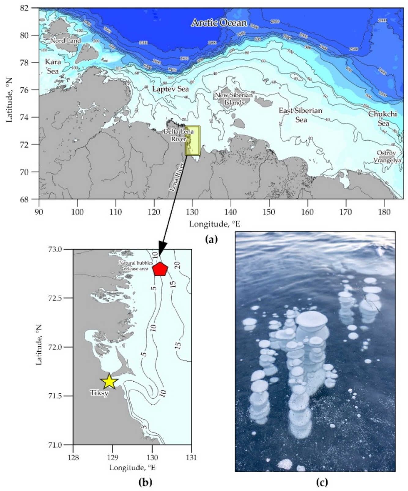
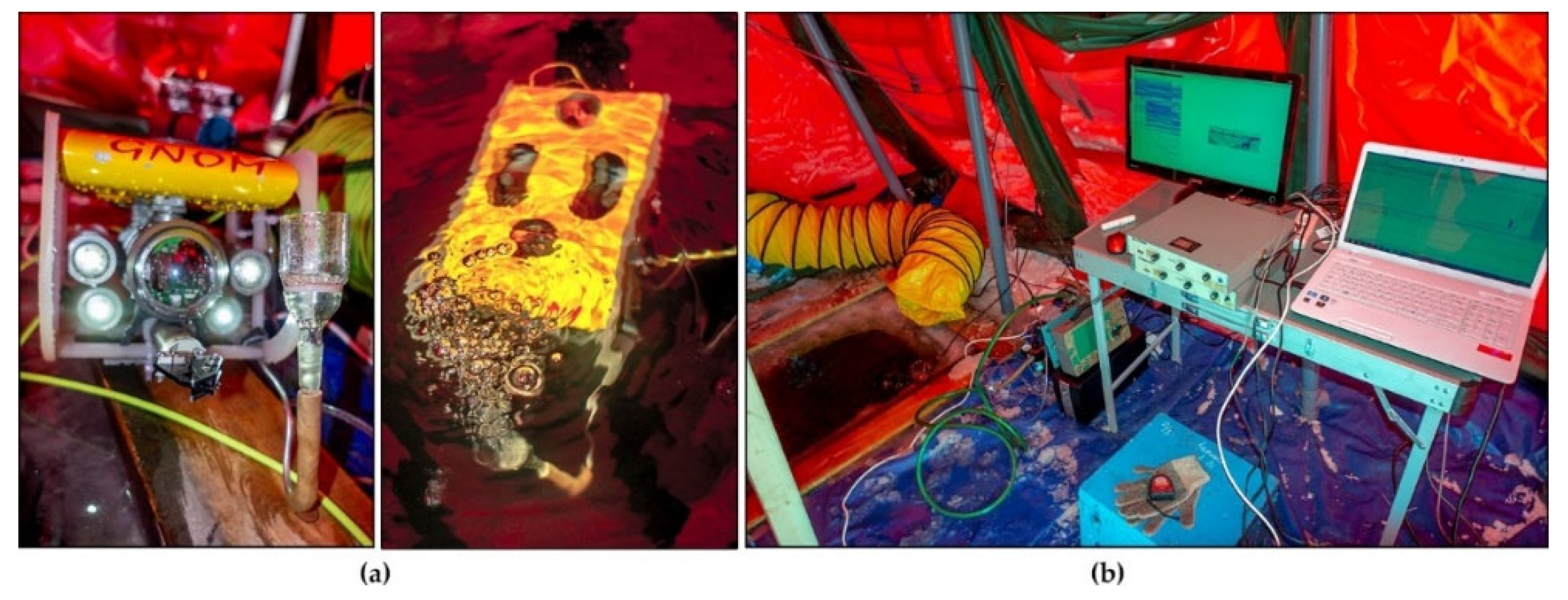
2. Materials and Methods

Quantification of CH4 bubble flux from sonar data is challenging and requires a comprehensive approach based on theoretical calculations, laboratory testing, field experiments and observations.
To obtain acoustic calibration of the echosounder in the shallow water, we conducted an in-situ experiment performed from the fast ice during the winter expedition in April 2012. In-situ calibration of an operational system allowed the measured echo level of a known acoustically insonified bubble volume to be directly related to the bubble flux rate. We recorded digital and acoustical images of: (1) artificially produced bubbles emitted from the tank installed on the fast ice surface in the tent lab (Figure 1) filled with gaseous CH4 under controlled conditions, and (2) natural bubbles and bubble streams at the actual seep site.
In the first part of the experiment, rates of fluxes and sizes of bubbles were maintained using a custom-made system modified after Ostrovsky et al. (2008) [13]. Compressed gas (nitrogen) was emitted via one or several Schott funnels installed in manipulator of the remotely operated underwater vehicle GNOM Standard (ROV GNOM), which was deployed to the sea bottom (Figure 2a). To receive a single bubble release, we used the Schott funnel (S2/210 × 575, Simax, Moscow, Russia) or nozzles. Bubbles were captured near the water surface using a large diameter inverse funnel submerged to the water beneath the sea ice at the seep site and connected to the sample rubber bladder also submerged to the water. This sampling technique was described in detail in [17]. After exposition in the water for 1 h, a sample bladder was removed from the water to examine the collected gas composition using gas chromatograph. Fraction of CH4 in the bubbles that reached the surface can be used to calculate actual CH4 flux rates (acoustical estimation corrected by fraction value) using acoustical technique described below.
Second part of the experiment was performed to detect, monitor and quantify ebullition rates in the water column. The multichannel hydroacoustic complex was designed using scientific single beam echosounder Furuno (Figure 2b) with a dual frequency of 50 and 200 kHz transducers and beam width of 12.5° and 2.5°, correspondingly. We estimated the CH4 bubble flux emitted from the seafloor into the water column by a method similar to that described in [14]. The main advantage of this approach is that the gas flux estimation does not require the knowledge of size, shape, and velocity of bubbles and the specifications of the echosounder. Our technique differs from that suggested in [14] in two key aspects: we used the field calibration rather than the laboratory one and the vertical insonification rather than the horizontal one. The calibration was performed from the fast ice in the “close to ideal” local field conditions (wind and wave induced noises were neglected), while the vertical transmission and reception of signals were chosen since the bubble flux was measured bottomward by ship-based echosounders. The measurements were run in the monostatic mode, as described in [4,14], when the sonic waves were emitted and received by the same electroacoustic transducer. In general, the applied approach was similar to the one performed ain the open sea echosounder calibration, which was described elsewhere [4,15,16]. To measure the bubble screen backscattering strength, the acoustic sensors were calibrated using a target provided by the manufacturer.
To estimate the bubble flow from the seafloor into the water column, a calibration test based on an experiment by Greinert and Nützel [14] on a dock with artificial nitrogen bubbles was performed as in [16,18]. The authors of [14] suggested that the level of backscattered sound signal from rising bubbles is uniquely determined by the gas flow volume carried by the bubbles, while the size of the bubbles, their number and emission methods can vary. The quantification of the CH4 flux in large water areas using the described method introduces an important advantage if compared with other quantification methods. This method only requires knowing the characteristics of the radiation pattern of the emitter and to perform calibration measurements of the dependence of the sound backscattering level on the gas flow carried by artificially generated bubbles. It has been shown that acoustical images of nitrogen bubbles are similar to those of methane bubbles [4,16,18].
The SRI 8610C series gas chromatograph (GC) equipped with a thermal conductivity detector (TCD; for N2, O2 (+Ar), CH4) and a flame ionization detector (FID; for CH4, CO2/with methanator, and C2–C5 hydrocarbons) was used to measure gas composition of bubbles floating from the bottom water/sediment interface up to the sea surface. The gas composition is shown in the Table 1. The GC was calibrated before each set of measurements using a three-point linear calibration line with three gas calibration standards. More details about this method can be found in [4,19,20,21].
To measure water currents and their direction, we used the Doppler current meter SonTek Argonaut XR. Small underwater remotely operated vehicle ROV GNOM Standard (Figure 2a) was used not only to deploy the gas tube to the bottom, but also to record videos and photos of the bubbles. Technical specifications of SonTek Argonaut XR and ROV GNOM Standard are presented in Table A1 (Appendix A). The upper end of that gas tube was connected to the nitrogen tank during calibration, and CH4 tank (mix, Table 1) for evaluation of CH4 fraction in bubbles reached the water column/sea ice interface, while the deepened end was equipped with the Schott glass filter funnels (Figure 2a).
The experiment was accomplished in slightly heated bottomless red tent, where multichannel system for digital hydroacoustical survey was located (Figure 2b). The fieldwork was performed using a large hole made in the ~2 m thick fast ice.

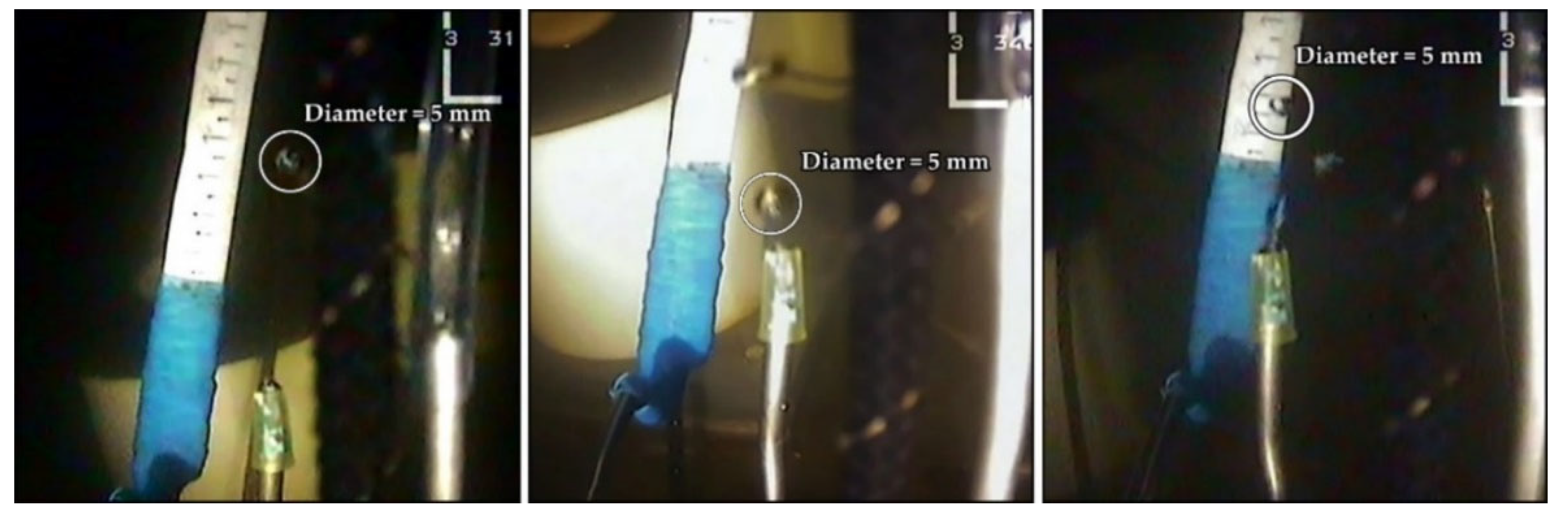
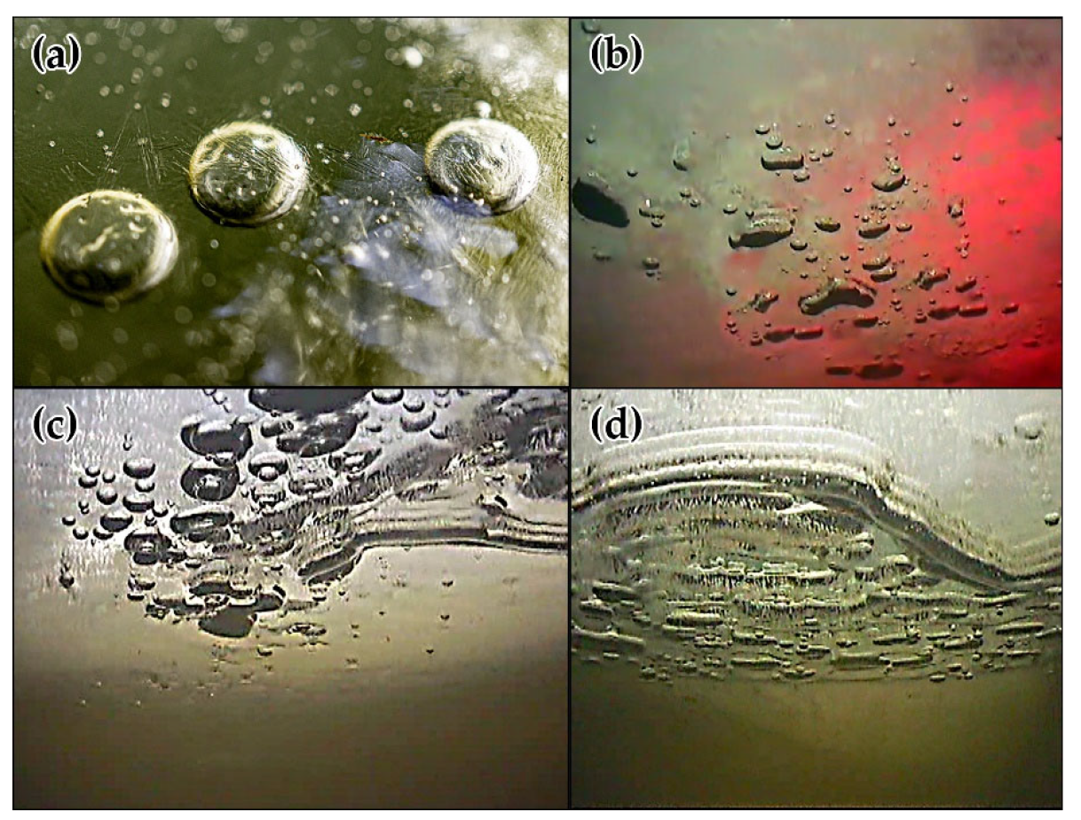
3. Results and Discussion

3.1. Bubble Composition

Because collecting bubbles in marine conditions, especially in the open water, is an extremely challenging task, we chose to work from the fast ice in the winter season, when seawater is calm, visibility is better than in the summer, and the sea ice prevents bubble escape to the atmosphere, which makes bubble collection feasible. We drilled a hole in the sea ice and created an artificial seep at ~8 m water depth; a gas tank with nitrogen as well as a gas tank with CH4 mix were installed on the fast ice. By tuning the valve (changing the pressure) installed on the gas tank head, bubble flow had been changing from 0.2 to 2.0 L per minute, creating a flow of ~5 mm diameter bubbles. Then, we captured bubbles escaping from the water surface using a chamber installed over the hole in the sea ice. After a one-hour exposure, we examined the composition of gas collected in the chamber and thus measured an actual CH4 flux from the water surface. Our data show that at the shallow water depth (8 m), ~67–72% (mean = 69.56%) of CH4 remains in the engineered bubbles with a diameter of ~5 mm, when the bubbles reach the sea surface (Table 1), while ~28–33% (mean = 30.5%) dissolve in the water column.
The experimental site was set up at a random location within the large area where increased concentrations of dissolved CH4 were observed earlier in both the summer and winter [3]. A square hole of 1 m2 was made in the 2 m thick sea ice and covered by a tent (Figure 2b). Visual observations of bubbles were performed using the ROV GNOM equipped with the high-speed video camera (Figure 2a). An example of a visual bubble recording is presented in Figure 3. Average visual bubble size (D) was about 5 ± 0.5 mm.
To visually examine and measure bubble sizes in the nearshore seepage area located close to several powerful CH4 hot spots [3,8] that were detected earlier, we drilled a hole in the fast ice. We observed and recorded bubble fluxes using the ROV deployed from another hole (3 m away from the first hole) and then allowed thin ice (4–6 cm) to form during the night (air temperature at night changed from −40 °C to −20 °C) so bubbles could not escape to the atmosphere. That allowed bubbles to be observed by the naked eye from above the ice and to be measured using a measuring tape. The low–medium seepage site was chosen based on a multiyear distribution of the dissolved CH4 concentrations [3,8] because of an opportunity to observe the flowing of single bubbles and groups of bubbles, which formed the flare-like shape. Observed individual bubble diameters ranged from 2 to 12.5 mm. Thus, these winter data revealed greater variability in bubble sizes than the data obtained during the summer marine investigation [4,7]. This could be due to the specific features of bubbles rising in the shallow water beneath the sea ice not dissolving but merging to create bubbles of greater size, as can be clearly seen in the photo made by the ROV (Figure 4). For the winter period, dissolved CH4 concentrations beneath the sea ice, increasing up to 2500–5000 nM, were 5 to 10 times higher than in the summer, when CH4 concentrations reached only ~200–800 nM [2,3,8]. We assume that high CH4 concentrations, accumulating beneath the sea ice, decrease the CH4 concentration gradient between the rising bubbles and surrounding water. Thus, bubbles may dissolve slower beneath the sea ice when compared to the summertime open water season, when the wind-driven mixing and dissolved CH4 ventilation occurs [8]. Storms enable more CH4 release because they destroy shallow water stratification and the mixed layer thickness increases many times owing to deep water mixing, thus increasing gas exchange across phase boundaries. As a result, bubble-mediated, storm-induced CH4 ‘pulses’ force a greater fraction of CH4 to bypass aqueous microbial ‘filters’ and reach the atmosphere [8,9].

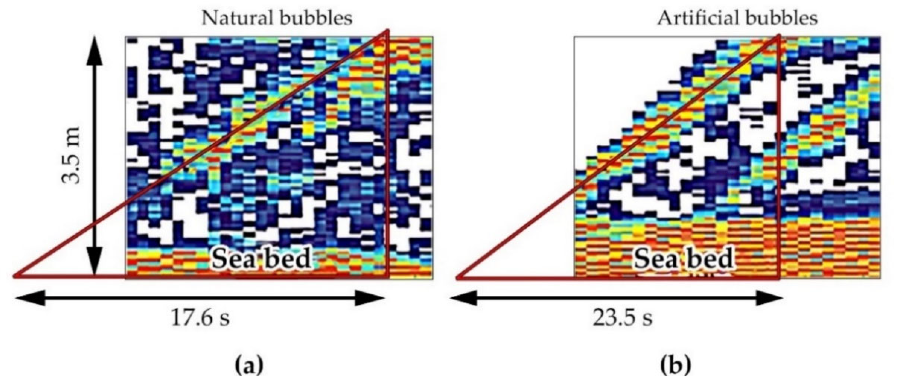
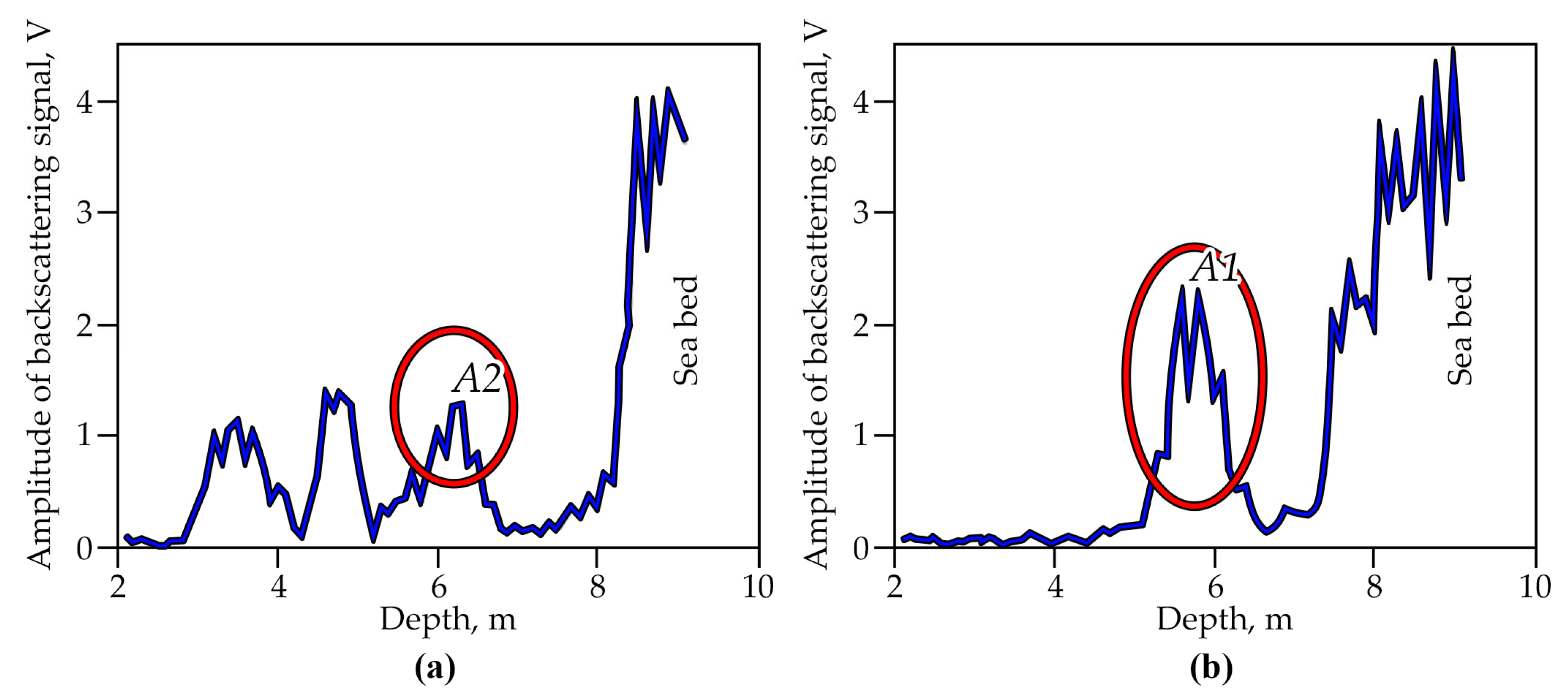
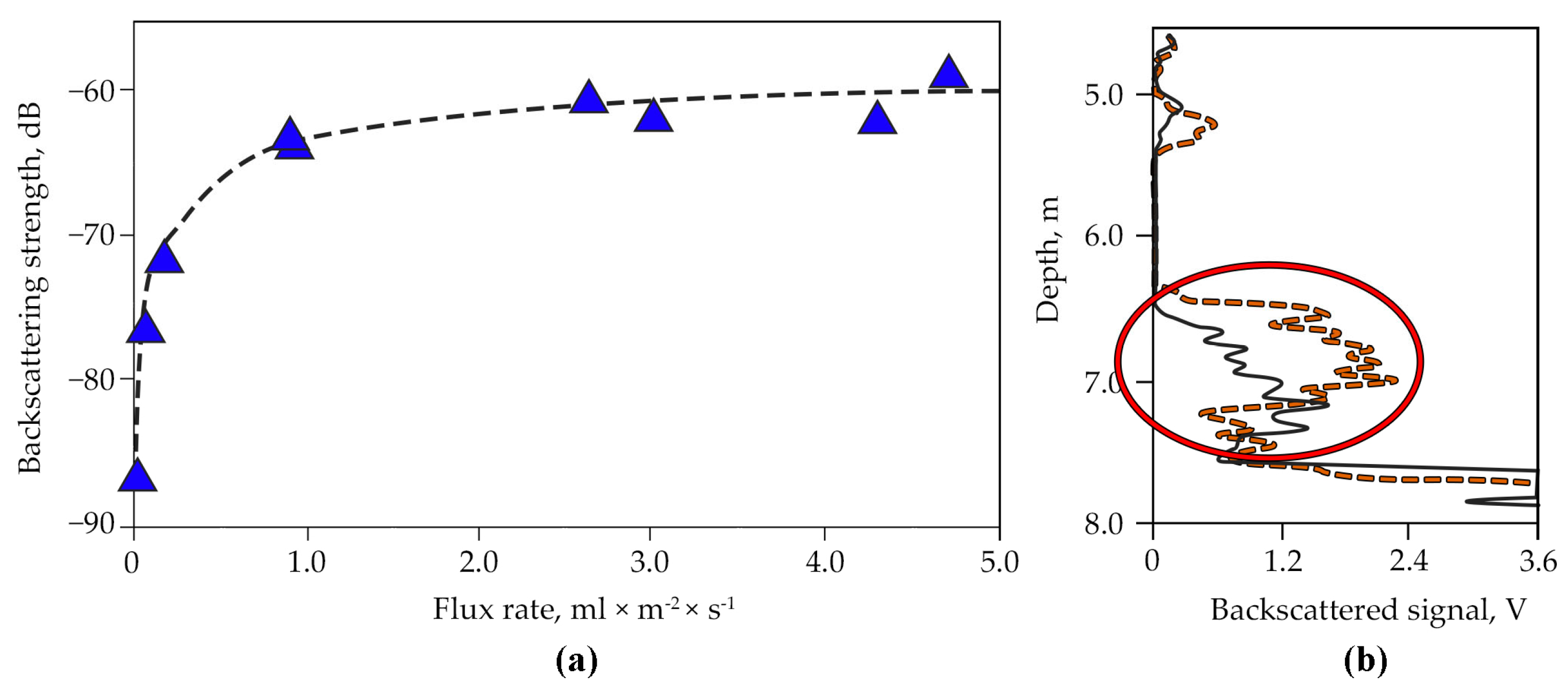
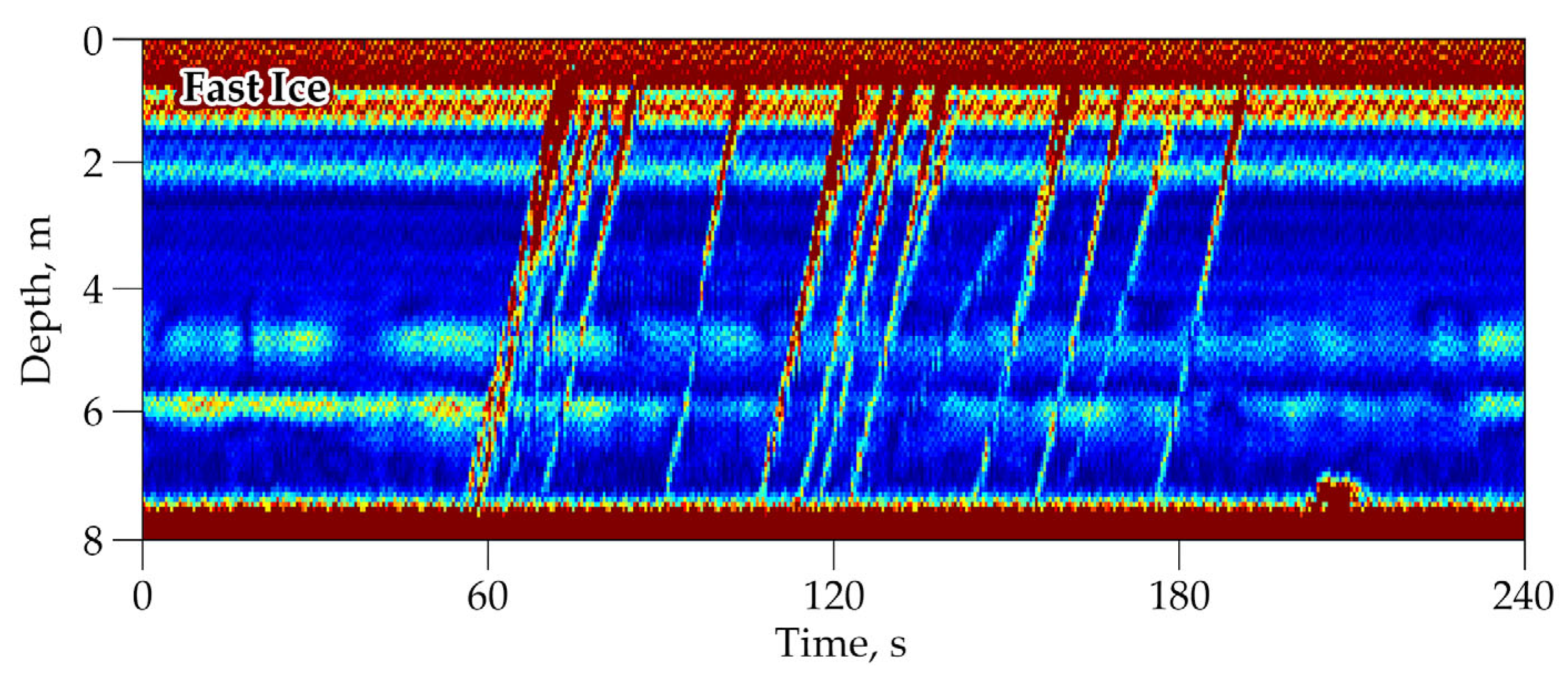
3.2. Acoustical Observations of Bubble Size and Flux

Bubble seeps were localized by the flare-like (after McGinnis et al., 2006 [22]) shape of the backscatter signal in the echogram. The backscattered signal of rising bubbles was continuously recorded digitally using a multichannel system for later digital analysis (Figure 5).
If the distance between the rising bubbles is more than half the length of the probing pulse, then they are displayed on the echogram separately as slanted lines. If the bubble, rising and moving horizontally due to the current, crossed the main lobe of the emitter radiation pattern, the average bubble ascent velocity (V) is determined using the expression [23]:
V = c o s ( φ ) × h t
where Δh is the difference in the depths of the visible ends of the bubble trajectory on the echogram, Δt is the corresponding time interval, and φ is the width of the radiation pattern ( φ = 25° for a 50 kHz transducer frequency). The ascent rate will be in the interval:
c o s ( φ ) × h t V h t
Estimated rise velocity for artificial bubbles was V1 ≈ 23 cm × s−1, for natural seep bubbles on-site V2 ≈ 18 cm × s−1 (Figure 6). Based on the rise velocity of floating up artificial and natural bubbles V1 and V2, their diameter (D) was determined using a plot presented in [22]. Visually observed and recorded D of artificial bubbles (D1 ≈ 5.0 ± 0.5 mm) together with estimated rise velocities fit well into the curves describing correlation between two parameters reported earlier in [22]. For natural bubbles, their D could be D1 ≈ 1.0 mm under the assumption that they are “clean” to D2 ≈ 5.6 mm under the assumption that they are “dirty” [24]. Bubble size estimation from rise velocities gives a bubble size range as follows:
1.0   m m   D 5.6   m m
Another method to evaluate the natural bubble size is using a cross-interpretation of backscatter signal amplitudes obtained for natural and artificial bubbles. The amplitude of the acoustic signal is proportional to the size of the floating up bubble [25]. As seen in Figure 7, the proportion between the amplitude of the backscattering signal of natural bubbles (A2) and the amplitude of the backscattering signal of artificial bubbles (A1) is A2/A1 ≈ 0.6. Under the assumption that bubbles are spherical, R~A, that means that D2/D1 ≈ 0.6, and D2 ≈ 3.0 ± 0.5 mm. As this size falls in the middle of the proposed range (1.0 mm ≤ D ≤ 5.6 mm), we can take this size as an average.
Calibration of the portable acoustic complex was carried out in conditions as close to natural as possible. To achieve this, artificial gas flares were created by using a gas tank with the CH4 mix (see Table 1) in the fast ice (Figure 1) bottom through the same hole, from which a gas flow of a given power was supplied through a nozzle into the water. The calibration was based on getting an empirical relationship between the backscattered sound signal from bubbles rising near the bottom and the amount of nitrogen, which is practically equal [16,18] to CH4 flow coming out of a nozzle installed directly under the radiator in the center of its radiation pattern (Figure 8a). Based on the calibration results using the least squares method, a correlation between the backscattering sound signal and the gas flow magnitude was plotted, and the natural flows of CH4 were then estimated. The values of the gas flow were recalculated into the flow from the bottom area unit (dimension mL × m−2 × s−1). To achieve this, the flow from the source, calculated in mL × s−1, was divided by the value of the effective area of the sounded zone at the bottom depth (for the configuration used, it is equal to 2 m2). The resulting calibration curve establishes a relationship between the backscattering of sound from bubbles at the bottom depth and the gas flow from 1 m2 of the bottom surface.
This calibration curve can be used to estimate small CH4 gas fluxes obtained with a single beam echosounder, in addition to the curve obtained by the same method for higher values of fluxes at the greater depths [4,15]. The calibration curve equation from Figure 8a is:
f x = p 1 × x + p 2
where f x is backscattering strength in dB, x —flux rate, mL × m−2 × s−1, and coefficients p 1 = 3.705 and p 1 = −63.66.
Video recordings of the calibration of a portable acoustic complex using an artificial gas flare showed that the average diameter of the bubbles rising from the outlet was 4.9 ± 0.3 mm. The resonant frequency of these bubbles is much less than the operating frequency of the echosounder (50 kHz), which satisfies the requirements for calibration described in [14]. During the experiment, it was found that the diameter of the gas bubbles rising from the nozzle weakly depends on the flow rate; it only affects the number of bubbles rising per unit time. Figure 8b exemplifies sound backscatter profiles for two bubble flows, 4 and 12 mL × s−1. It can be seen that the area with bubbles occupies a depth section of 7.5–6.5 m, and the level of sound backscattering increases with increasing gas flow. Figure 8a shows the calibration curve of sound backscatter versus gas flow. In a wide range of flow values changing from 0.02 to 4.7 mL × m−2 × s−1, this dependence is linear, so the calibration factor was used for further calculations of the natural gas flows.
During observations of natural bubbles, we detected three periods of their increased activity (lasting from 5 to 15 min) with a total of 63 short-term ejections of bubbles from the seabed. Figure 9 shows typical examples of echograms with bubbles rising from the seabed. The trajectories of rising bubbles at the moments of ejections are displayed on the echogram as straight lines from the bottom to the surface. The slope of these lines is mainly determined by the bubble ascent rate, which is 20 ± 2 cm/s for the registered bubbles. The average duration of one short burst is 2.0 ± 0.4 s.
Acoustic observations have shown that rising bubbles are emitted from the seabed extremely unevenly: short term periods of increased activity alternated with rather long periods when no release of gas bubbles from the bottom was observed. The intervals between the periods of their increased activity were about 2.5 h, which approximately corresponds to the period of recorded internal waves, causing fluctuations in the current velocity at the different horizons (Figure 10). During the bubbles’ release from the seabed, the current velocities at the lower horizons (5 and 7 m) were minimal and did not exceed 10 cm·s−1, which is illustrated in Figure 10. Estimates based on the obtained calibration factor showed that the CH4 flux due to bubble transfer from the bottom reached 4.4 mL × m−2 × s−1 at the moments of the short-term emissions, with an average flow of 0.3 mL × m−2 × s−1, which is equal to the average value of CH4 ebullition ~19 g × m−2 per day. We might consider this value as the first quantitative on-site estimation of the CH4 ebullition from the seafloor at the hot spot discovered in September 2005, and then surveyed almost annually [2,3,6]. The gas exchange between bubbles and water depends on the bubble size, its shape, and water temperature, so the resulting CH4 flux to the sea surface and atmosphere could be different. Therefore, in order to move from estimating the CH4 flux entering the water column at the bottom/seawater interface to estimating the CH4 flux transported by rising bubbles to the water/sea ice interface, we need to consider the magnitude of gas exchange between the rising bubbles and the water column, through which the bubbles rise. As shown earlier, ~67–72% (mean = 69.56%) of CH4 beneath 2 m thick ice remains in the engineered bubbles with a diameter of ~5 mm, which corresponds to 80% of its initial concentration (Table 1). Considering this value, the CH4 flux transported by the bubbles to the water/sea ice interface is estimated to be about 15 g × m−2 of CH4 per day. It should be noted that this bubble-transported CH4 flux reaching the water surface can be emitted from the water/sea ice interface directly into the atmosphere via polynyas, leads and ice trenches.
This value is in the mid high range of CH4 ebullition values estimated for the entire ESAS [4], and two orders higher than the upper range of CH4 ebullition from the typical and well-studied Low Arctic/Subarctic thermocarst lakes. Ebullition rates from the Low Arctic/Subarctic lakes (Chersky area, the Kolyma lowland) are supposed to be about 100 times higher than in the High Arctic lakes (Tiksy area, near the Buor–Khaya Bay), according to the contrasting concentrations of dissolved CH4 for these study sites [17,26,27]. The wintertime results also confirm previous multi-year summertime data obtained in the entire ESAS showing much higher rates of CH4 ebullition in comparison with other Arctic areas such as offshore Svalbard, which was also heavily studied in terms of CH4 fluxes, variations, and bubble fluxes [28,29,30].
In our previous work we found that the maximal CH4 value of ebullition in the thermocarst (or thaw, by origin) lake (Schuchie lake located in the Kolyma lowland) was obtained after drastic CH4 release correlated with a low-air-pressure event. All sites, including shallow water sites, showed a remarkable synchrony in the bubble release correlated with changes in local air pressure with a small change in the total pressure at the bottom [26]. For instance, the cross moving of a cyclone with an air pressure drop to 740 Torr increases the mean value of CH4 ebullition from background values ranging between ~15–50 mg × m−2 × d−1 up to 200–300 mg × m−2 × d−1 at the lake site with a depth of ~10 m—similar to depth at this study site (~8 m) [26,27]. Hence, the cross moving of cyclonic systems might trigger the CH4 efflux from the northern lakes. In frame of our experiment accomplished on the fast ice, we tried to find a link between current velocities measured at two horizons (5 m and 7 m) and the CH4 ebullition rates (Figure 10). We suggest that the higher rates of CH4 ebullition on-site might be related to a decrease in water current values of the dynamic water pressure near the bottom (horizon 7 m): two successful cases (near 7 h, near 11.5 h) vs. one unsuccessful case (near 9 h). Perhaps, an increase in CH4 ebullition for the latter case could be associated with an atmospheric pressure drop. At this stage, we plan to perform additional experimental and field studies to better understand the mechanism of small “pressure triggers” vs. changing CH4 ebullition.

4. Conclusions

This paper presents the first quantitative estimate of the CH4 flux transported by rising bubbles from a depth of 8 m, obtained in the shallow ESAS in wintertime at two levels of the water column: (1) at the bottom/seawater interface, and (2) at the water/sea ice interface. In total, 63 short-term bubble ejections were registered during the observations (about 10 h). In the case of longer observations, the number of detected short-term bubble emissions could increase.
The observed wintertime natural individual bubble diameter ranged from 2 to 12.5 mm, meaning that the summertime average size (diameter = 7.5 mm) fits well to the range of natural bubbles observed in this study. Winter data revealed greater variability in the bubble sizes than the data obtained during the summer marine investigation. This could be due to the specific features of bubbles rising in the shallow water beneath the sea ice where merging bubbles create bubbles of greater size.
It was shown that the CH4 flux from the seabed to the near-bottom water layer (bottom/seawater interface) was ~19 g × m−2 per day. Our data indicated that ~67–72% (mean = 69.56%) of CH4 accumulated beneath 2 m thick ice at the shallow water depth (8 m) remains in the engineered bubbles with a diameter of ~5 mm, which corresponds to 80% of its initial concentration (Table 1). Considering this value, the CH4 flux transported by the bubbles to the water/sea ice interface is estimated to be about 15 g × m−2 of CH4 per day. We suggest that this bubble-transported CH4 flux reaching the water surface can be emitted from water/sea ice interface directly into the atmosphere via polynyas, leads and ice trenches. A specific feature of the ESAS is that during the winter, about 10% of the shelf area is composed of open water (and young ice off the land-fast ice) or polynyas, which are parts of the Great Siberian Polynya [21]. Followed by land-fast ice formation, polynyas develop in November when the wind breaks apart the fast ice and the drifting sea ice propagates hundreds of kilometers offshore [22].
This CH4 ebullition value detected at the water/sea ice interface is also in the mid high range of CH4 ebullition values estimated for the entire ESAS [4], and two orders higher than upper range of CH4 ebullition from the typical Low Arctic/Subarctic thermocarst (thaw) lakes. Note, that ebullition rates from the Low Arctic/Subarctic lakes (Chersky area, the Kolyma lowland) are supposed to be about 100 times higher than in High Arctic lakes (Tiksy area, near the Buor–Khaya Bay) because such a difference was found in their CH4 concentrations [27,31]. Thus, the total CH4 ebullition from the vast shallow ESAS are supposed to be significantly higher than from the northern thermocarst lakes, which are considered to be a source of CH4 of global significance [17].

Author Contributions

Conceptualization, N.S., D.C. and I.S.; methodology, D.C., V.Y. and I.S.; software, D.C. and V.Y.; validation, D.C. and I.S.; formal analysis, D.C. and V.Y.; investigation, all authors; resources, I.S. and N.S.; data curation, D.C.; writing—original draft preparation, D.C., E.G. and I.S.; writing—review and editing, N.S. and E.G.; visualization, D.C.; supervision, N.S. and V.Y.; project administration, I.S. and B.M.; and funding acquisition, I.S., B.M. and N.S. All authors have read and agreed to the published version of the manuscript.

Funding

The article was prepared in the framework of a research grant funded by the Ministry of Science and Higher Education of the Russian Federation (grant ID: 075-15-2022-325).

Institutional Review Board Statement

Not applicable.

Informed Consent Statement

Not applicable.

Data Availability Statement

Not applicable.

Acknowledgments

We thank the collaborating partners and everyone else involved in the over–ice expeditions in the Laptev Sea (April 2007, 2012) that contributed technically to the first quantitative estimation of CH4 ebullition release in the ESAS nearshore zone. Special thanks to Oleg Dudarev, Alexander Salomatin (POI and TSU), and Dmitry Melnichenko (Tiksy Hydrobase) for their valuable support.

Conflicts of Interest

The authors declare no conflict of interest.

Appendix A

Table A1. SonTek Argonaut XR and GNOM Standard technical specifications.
Acoustic Doppler Current Profilers ADCPs and Current Meters
Profiling Feature
Frequency1.5 MHz
Max Profiling Range20.0 m (66.0 ft)
Min Cell Size0.40 m (1.2 ft)
Min Blanking Distance0.50 m (1.6 ft)
Main Measurement Cell
Cell Begin (CB)Min 0.50 m(1.6 ft)
Max 19.5 m(63.4 ft)
Cell End (CE)Min 1.50 m (4.9 ft)
Max 20 m (66.0 ft)
Min CE–CB1.00 m (3.28 ft)
Velocity (Main measurement cell plus up to 10 cells in profiling feature)
Range±6 m/s
Resolution0.1 cm/s
Accuracy±1% of measured velocity, ±0.5 cm/s
Compass/Tilt Sensor
Calibration ProcedureBuilt–in, compensate for ambient magnetic fields
Resolution0.1°
Heading Accuracy±2°
Pitch, Roll Accuracy±1°
Temperature
Resolution0.01 °C
Accuracy±0.1 °C
PressurePiezoresistive strain gauge, 0.1% accuracy
Recorder Size4 MB
Environmental
Pressure Rating200 m (pressure sensor dependent)
Operating Temperature−5° to 40 °C
Storage Temperature−10° to 50 °C
Physical
HousingDelrin plastic
Weight in Air2.5 kg|5.5 lb.
Weight in Water−0.3 kg|−0.7 lb.
Dimensions15.2 cm × 18.0 cm|6.0 in × 7.1 in
Power
Input Power7–15 V DC
Typical Power Consumption0.2 to 0.5 W Continuous; 0.01 W Stand–by
CommunicationsRS232, SDI–12
Small underwater remotely operated vehicle GNOM Standard
Underwater part
Maximum Operating depthup to 150 m
Dimensions (L × W × H) 350 mm × 200 mm × 200 mm
Weight in air / total system weight3 kg/12 kg
Thrusters3 magnetically coupled DC motors
Horizontal: 2× thrusters, 24 VDC 16W
Vertical: 1× thruster, 24 VDC 16W
Cruising speedup to 3 knots
Camera system
Camera ModelSony Super HAD 2 CCD
Camera resolution700 TV Lines
Image Sensor1/3″ Interline Transfer CCD
Mini Illumination0.1 lux (0.01 − b/w camera)
Lens3.6 mm/F2.0
Iris ControlAuto
FocusAuto
Field of View (FOV)66°
Camera Tilt±50°
Lighting system
Light SourceWhite ultra–bright LEDs
Luminous Flux400 lumens
Beam Angle105°
Color Temperature5600–6000° Kelvin
ControlVariable intensity
Navigation system
SensorsCompass and Depth
Heading Accuracy±3°
Compass Resolution0.5°
Depth Sensor Accuracy1% F.S.

References

  1. Schuur, E.A.G.; McGuire, A.D.; Schädel, C.; Grosse, G.; Harden, J.W.; Hayes, D.J.; Hugelius, G.; Koven, C.D.; Kuhry, P.; Lawrence, D.M.; et al. Climate change and the permafrost carbon feedback. Nature 2015, 520, 171–179. [Google Scholar] [CrossRef] [PubMed]
  2. Shakhova, N.; Semiletov, I.; Leifer, I.; Salyuk, A.; Rekant, P.; Kosmach, D. Geochemical and geophysical evidence of methane release over the East Siberian Arctic Shelf. J. Geophys. Res. Space Phys. 2010, 115, 14. [Google Scholar] [CrossRef]
  3. Shakhova, N.; Semiletov, I.; Salyuk, A.; Yusupov, V.; Kosmach, D.; Gustafsson, Ö. Extensive Methane Venting to the Atmosphere from Sediments of the East Siberian Arctic Shelf. Science 2010, 327, 1246–1250. [Google Scholar] [CrossRef] [PubMed]
  4. Shakhova, N.; Semiletov, I.; Sergienko, V.; Lobkovsky, L.; Yusupov, V.; Salyuk, A.; Salomatin, A.; Chernykh, D.; Kosmach, D.; Panteleev, G.; et al. The East Siberian Arctic Shelf: Towards further assessment of permafrost-related methane fluxes and role of sea ice. Philos. Trans. R. Soc. A Math. Phys. Eng. Sci. 2015, 373, 20140451. [Google Scholar] [CrossRef]
  5. Steinbach, J.; Holmstrand, H.; Shcherbakova, K.; Kosmach, D.; Brüchert, V.; Shakhova, N.; Salyuk, A.; Sapart, C.J.; Chernykh, D.; Noormets, R.; et al. Source apportionment of methane escaping the subsea permafrost system in the outer Eurasian Arctic Shelf. Proc. Natl. Acad. Sci. USA 2021, 118, e2019672118. [Google Scholar] [CrossRef] [PubMed]
  6. Vonk, J.E.; Sánchez-García, L.; Van Dongen, B.E.; Alling, V.; Kosmach, D.; Charkin, A.; Semiletov, I.P.; Dudarev, O.V.; Shakhova, N.; Roos, P.; et al. Activation of old carbon by erosion of coastal and subsea permafrost in Arctic Siberia. Nature 2012, 489, 137–140. [Google Scholar] [CrossRef]
  7. Shakhova, N.; Semiletov, I.; Gustafsson, O.; Sergienko, V.; Lobkovsky, L.; Dudarev, O.; Tumskoy, V.; Grigoriev, M.; Mazurov, A.; Salyuk, A.; et al. Current rates and mechanisms of subsea permafrost degradation in the East Siberian Arctic Shelf. Nat. Commun. 2017, 8, 15872. [Google Scholar] [CrossRef] [Green Version]
  8. Shakhova, N.; Semiletov, I.; Leifer, I.; Sergienko, V.; Salyuk, A.; Kosmach, D.; Chernykh, D.; Stubbs, C.; Nicolsky, D.; Tumskoy, V.; et al. Ebullition and storm-induced methane release from the East Siberian Arctic Shelf. Nat. Geosci. 2014, 7, 64–70. [Google Scholar] [CrossRef]
  9. Shakhova, N.; Semiletov, I.; Chuvilin, E. Understanding the Permafrost–Hydrate System and Associated Methane Releases in the East Siberian Arctic Shelf. Geosciences 2019, 9, 251. [Google Scholar] [CrossRef] [Green Version]
  10. Dean, J.F.; Middelburg, J.J.; Röckmann, T.; Aerts, R.; Blauw, L.G.; Egger, M.; Jetten, M.S.M.; de Jong, A.E.E.; Meisel, O.H.; Rasigraf, O.; et al. Methane Feedbacks to the Global Climate System in a Warmer World. Rev. Geophys. 2018, 56, 207–250. [Google Scholar] [CrossRef] [Green Version]
  11. Hugelius, G.; Strauss, J.; Zubrzycki, S.; Harden, J.; Schuur, E.; Ping, C.-L.; Schirrmeister, L.; Grosse, G.; Michaelson, G.; Koven, C.; et al. Estimated stocks of circumpolar permafrost carbon with quantified uncertainty ranges and identified data gaps. Biogeosciences 2014, 11, 6573–6593. [Google Scholar] [CrossRef] [Green Version]
  12. Romanovskii, N.N.; Hubberten, H.-W.; Gavrilov, A.V.; Eliseeva, A.A.; Tipenko, G.S. Offshore permafrost and gas hydrate stability zone on the shelf of East Siberian Seas. Geo-Mar. Lett. 2005, 25, 167–182. [Google Scholar] [CrossRef] [Green Version]
  13. Ostrovsky, I.; McGinnis, D.F.; Lapidus, L.; Eckert, W. Quantifying gas ebullition with echosounder: The role of methane transport by bubbles in a medium-sized lake. Limnol. Oceanogr. Methods 2008, 6, 105–118. [Google Scholar] [CrossRef] [Green Version]
  14. Greinert, J.; Nutzel, B. Hydroacoustic experiments to establish a method for the determination of methane bubble fluxes at cold seeps. Geo-Mar. Lett. 2004, 24, 75–85. [Google Scholar] [CrossRef]
  15. Chernykh, D.; Yusupov, V.; Salomatin, A.; Kosmach, D.; Shakhova, N.; Gershelis, E.; Konstantinov, A.; Grinko, A.; Chuvilin, E.; Dudarev, O.; et al. Sonar Estimation of Methane Bubble Flux from Thawing Subsea Permafrost: A Case Study from the Laptev Sea Shelf. Geosciences 2020, 10, 411. [Google Scholar] [CrossRef]
  16. Leifer, I.; Chernykh, D.; Shakhova, N.; Semiletov, I. Sonar gas flux estimation by bubble insonification: Application to methane bubble flux from seep areas in the outer Laptev Sea. Cryosphere 2017, 11, 1333–1350. [Google Scholar] [CrossRef] [Green Version]
  17. Semiletov, I.P.; Pipko, I.; Pivovarov, N.Y.; Popov, V.V.; Zimov, S.A.; Voropaev, Y.V.; Daviodov, S.P. Atmospheric carbon emission from North Asian Lakes: A factor of global significance. Atmos. Environ. 1996, 30, 1657–1671. [Google Scholar] [CrossRef]
  18. Leifer, I.; Culling, D. Formation of seep bubble plumes in the Coal Oil Point seep field. Geo-Mar. Lett. 2010, 30, 339–353. [Google Scholar] [CrossRef]
  19. Yusupov, V.; Salomatin, A.; Shakhova, N.; Chernykh, D.; Domaniuk, A.; Semiletov, I. Echo Sounding for Remote Estimation of Seabed Temperatures on the Arctic Shelf. Geosciences 2022, 12, 315. [Google Scholar] [CrossRef]
  20. Shakhova, N.; Semiletov, I. Methane release and coastal environment in the East Siberian Arctic shelf. J. Mar. Syst. 2007, 66, 227–243. [Google Scholar] [CrossRef]
  21. Shakhova, N.; Semiletov, I.; Panteleev, G. The distribution of methane on the Siberian Arctic shelves: Implications for the marine methane cycle. Geophys. Res. Lett. 2005, 32, L09601. [Google Scholar] [CrossRef]
  22. McGinnis, D.F.; Greinert, J.; Artemov, Y.; Beaubien, S.E.; Wüest, A. Fate of rising methane bubbles in stratified waters: How much methane reaches the atmosphere? J. Geophys. Res. Atmos. 2006, 111, 15. [Google Scholar] [CrossRef] [Green Version]
  23. Salomatin, A.S.; Yusupov, V.I. Acoustic investigations of gas “flares” in the Sea of Okhotsk. Oceanology 2011, 51, 857–865. [Google Scholar] [CrossRef]
  24. Clift, R.; Grace, J.R.; Weber, M.E. Bubbles, drops, and particles. Dry. Technol. 1978, 11, 263–264. [Google Scholar]
  25. Medwin, H.; Clay, C.S. Fundamentals of Acoustical Oceanography; Elsevier Science: Amsterdam, The Netherlands, 1997. [Google Scholar]
  26. Semiletov, I.P.; Pivovarov, N.Y.; Pipko, I.I.; Gukov, A.Y.; Volkova, T.I.; Sharp, J.P.; Shcherbakov, Y.S.; Fedorov, K.P. Dynamics of dissolved CH4 and CO2 in the Lena River Delta and Laptev Sea. Trans. Dokl. Russ. Acad. Sci. 1996, 350, 401–404. [Google Scholar]
  27. Semiletov, I.P.; Zimov, S.A.; Voropayev, Y.V.; Davydov, S.P.; Barkov, N.A.; Gusev, A.M.; Lipenkov, V.Y. Atmospheric methane in the past and present. Dokl. Earth Sci. 1994, 343, 155–159. [Google Scholar]
  28. Veloso, M.; Greinert, J.; Mienert, J.; De Batist, M. A new methodology for quantifying bubble flow rates in deep water using splitbeam echosounders: Examples from the Arctic offshore NW-Svalbard. Limnol. Oceanogr. Methods 2015, 13, 267–287. [Google Scholar] [CrossRef] [Green Version]
  29. Jansson, P.; Triest, J.; Grilli, R.; Ferré, B.; Silyakova, A.; Mienert, J.; Chappellaz, J. High-resolution underwater laser spectrometer sensing provides new insights into methane distribution at an Arctic seepage site. Ocean Sci. 2019, 15, 1055–1069. [Google Scholar] [CrossRef] [Green Version]
  30. Ferré, B.; Jansson, P.; Moser, M.; Serov, P.; Portnov, A.; Graves, C.A.; Panieri, G.; Gründger, F.M.L.; Berndt, C.; Lehmann, M.F.; et al. Reduced methane seepage from Arctic sediments during cold bottom-water conditions. Nat. Geosci. 2020, 13, 144–148. [Google Scholar] [CrossRef]
  31. Semiletov, I.; Makshtas, A.; Akasofu, S.-I.; Andreas, E.L. Atmospheric CO2 balance: The role of Arctic Sea ice. Geophys. Res. Lett. 2004, 31, L05121. [Google Scholar] [CrossRef]
Figure 1. Map of East Siberian Arctic Shelf with selected yellow rectangle research area (a); map of the work area with the location of the natural CH4 bubble release area marked (red pentagon) and the Tiksy village where the expedition started (yellow star) (b); the sample of bubbles frozen into fast ice near CH4 bubble release area from figure b (c).
Geosciences 13 00228 g001
Figure 2. Underwater remotely operated vehicle with Schott glass funnels (a); set up of the experimental site: a multichannel system for digital hydroacoustical data recording installed in close proximity to the hole made in the sea ice, where bubble observation was performed (b).
Geosciences 13 00228 g002
Figure 3. Examples single artificial rising bubbles with diameter D = 5 ± 0.5 mm. The rising bubble enclosed in a circle.
Geosciences 13 00228 g003
Figure 4. Examples of bubbles observed in the sea ice and in the water column beneath the sea ice. Single flowing bubbles entrapped by the sea ice (a). Bubbles stacking into the sea ice and starting merging into larger size bubbles (bd).
Geosciences 13 00228 g004
Figure 5. Examples of echogram attributed to natural seep bubbles (a) and artificially made bubbles (b) recorded with 50 kHz transducer frequency (red arrows and circles mark particular bubbles to which further estimates are attributed).
Geosciences 13 00228 g005
Figure 6. Fragments of echogram used to evaluate bubble rise velocities of natural seep bubbles (a) and artificial bubbles (b). Red triangles demonstrated the method used.
Geosciences 13 00228 g006
Figure 7. Example of amplitude (A) of backscattering signal recorded for natural seep bubbles (a) and artificial bubbles (b) (red ovals mark bubble for which estimate was made).
Geosciences 13 00228 g007
Figure 8. Calibration curve built from the results of calibration measurements (indicated by triangles) (a). Sound backscatter profiles for two givens nitrogen/CH4 flows at calibration (b). The solid line corresponds to a flow of 2 mL × m−2 × s−1, the dashed line corresponds to 6 mL × m−2 × s−1. An ellipse marked the area near the bottom with gas bubbles.
Geosciences 13 00228 g008
Figure 9. Fragments of echogram of natural seep bubbles recorded in the study area.
Geosciences 13 00228 g009
Figure 10. CH4 fluxes (points) and flow velocities at different horizons. Arrows indicate periods of increased CH4 ebullition. Green circles—rising natural bubbles; blue line—stream velocity changed over time at a depth of 5 m; red dashed line—stream velocity changed over time at a depth of 7 m.
Geosciences 13 00228 g010
Table 1. Gas composition of bubbles floating from the bottom water/sediment interface up to the sea surface (measured by gas chromatograph).
Gas Mixture ComponentsGas Components in Bubbles
near the Seabed, %
Gas Components in Bubbles
near the Sea Surface, %
O21.86.24
N29.1723.36
CH485.2269.56
CO23.710.76
Disclaimer/Publisher’s Note: The statements, opinions and data contained in all publications are solely those of the individual author(s) and contributor(s) and not of MDPI and/or the editor(s). MDPI and/or the editor(s) disclaim responsibility for any injury to people or property resulting from any ideas, methods, instructions or products referred to in the content.

