
Landslide Susceptibility Analysis by Applying TRIGRS to a Reliable Geotechnical Slope Model
by
 , ,
, ,
Mariantonietta Ciurleo
1, 
Settimio Ferlisi
2,
Vito Foresta
2,
Maria Clorinda Mandaglio
2,* and
Nicola Moraci
1,* 1
Department of Civil, Energy, Environmental and Materials Engineering, Mediterranea University of Reggio Calabria, Via Graziella—Feo di Vito, 89124 Reggio Calabria, Italy
2
Department of Civil Engineering, University of Salerno, Via Giovanni Paolo II, 84084 Fisciano, Italy
*
Authors to whom correspondence should be addressed.
Geosciences 2022, 12(1), 18; https://doi.org/10.3390/geosciences12010018
Submission received: 7 December 2021
/
Revised: 21 December 2021
/
Accepted: 29 December 2021
/
Published: 31 December 2021
(This article belongs to the Section Natural Hazards)
Abstract
:This paper presents the results of a research aimed at analysing the susceptibility to shallow landslides of a study area in the Calabria region (Southern Italy). These shallow landslides, which in some cases evolve as debris flows, periodically affect the study area, causing damage to structures and infrastructure. The involved soils come from the weathering of gneissic rocks and cover about 60% of the study area. To fulfil the goal of the research, the Transient Rainfall Infiltration and Grid-based Slope-Stability (TRIGRS) model was first used, assuming input data (including physical and mechanical parameters of soils) provided by the scientific literature. Then, the preliminary results obtained were used to properly locate in situ investigations that included sampling. Geotechnical laboratory tests allowed characterising the investigated soils, and related parameters were used as new input data of the TRIGRS model. The generated shallow landslide susceptibility scenario showed a good predictive capability based on the adoption of a cutoff-independent performance technique.
1. Introduction
Landslide risk management is a complex process that first involves analysing the risk [1]. Risk analysis is comprised of different consequential steps that ordinately deal with susceptibility, hazard and consequence analyses; finally, the risk is estimated. Focusing on susceptibility analysis, specifically aimed to determine the spatial probability pertaining to a given type of landslides in a certain area, methods to be adopted can be heuristic or knowledge-based, empirical/statistical and deterministic/probabilistic according to the scale of zoning, provided that predisposing factors are properly identified [2,3,4,5,6]. At large (1:25,000 to 1:5000) and detailed (>1:5000) scales, adopting deterministic/probabilistic methods allows simulating the physical process that governs the triggering mechanism of investigated landslides, based on an accurate geotechnical characterization of the involved soils.
This work focuses on the susceptibility analysis at a large scale (1:5000) to (the occurrence of) rainfall-induced first-time shallow landslides that, during the propagation stage, can be rich with high kinetic energy values to cause detrimental effects on the exposed elements located in piedmont areas [7,8,9,10,11,12]. To this aim, we applied the “Transient Rainfall Infiltration and Grid-based Slope-Stability” (TRIGRS) deterministic model to a study area in the Calabria region (Southern Italy), which is periodically affected by rainfall-induced shallow landslides later propagating as debris flows, being the exposed facilities some linear infrastructure.
The investigated shallow landslides involve a weathered crystalline (gneissic) rock. The shear failure surfaces are generally located along the contact between residual, colluvial or detrital soils (gneiss of weathering grade or class VI) and relatively less weathered gneissic rock [13,14]. Owing to their inherent heterogeneity, related hydraulic or mechanical parameter values are characterised by a marked variability, as highlighted by the limited scientific literature on the topic [8,9,11,15,16]. Therefore, using tout court, the available information in performing TRIGRS analyses may lead to inaccurate results, mainly if the same information deals with soils of nearby areas not directly involved in the shallow landslides under consideration. To overcome these difficulties, in this work, preliminary results obtained by the TRIGRS model on the study area using input data obtained from the scientific literature were first valorised to identify the sites where in situ investigations and sampling activities must be performed. Then, laboratory tests were carried out to characterise, from a geotechnical point of view, the soils specifically involved in the investigated shallow landslides and, accordingly, properly define the input data of TRIGRS. This allows obtaining an accurate shallow landslide susceptibility map, of which the predictive capability can be proved based on the adoption of a cutoff-independent performance technique, such as those leading to the generation of receiver-operating characteristic (ROC) curves [17].
2. Materials and Methods
2.1. Study Area and Landslide Inventory Map
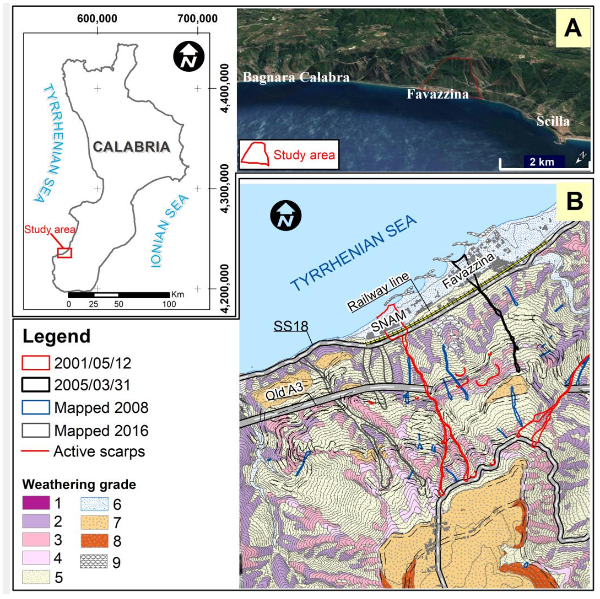
The study area is located within the Costa Viola between the villages of Scilla and Bagnara Calabra (Figure 1A). It extends for about 1 km2 and is bordered at the top by “Piano delle Aquile” (a flat area of marine origin) and at the bottom by a densely urbanized coastal plain including the Favazzina village (Figure 1A).
From a geological point of view, the paleozoic basement of the area is manly constituted by high-grade metamorphic rocks (para- and ortho-gneiss), overlapped by Upper Pliocene to Holocene sedimentary deposits [18,19]. The Paleozoic crystalline basement shows strongly tectonised and intense deeply weathered conditions [18]. Particularly, six weathering classes can be recognized in the study area. Moving from the bottom to the top, the weathering sequence consists of a slightly weathered rock (weathering class II) superimposed by a moderately weathered rock (weathering class III), which rarely outcrops, whereas a highly weathered rock (weathering class IV) outcrops in the middle-lower part of the slope. Completely weathered rock or saprolite (weathering class V) prevails in the upper part of the slope along with residual, colluvial and detrital soils (weathering class VI), which covers about the 60% of the study area.
In the study area, rainfall-induced landslides periodically occur involving the gneiss of different weathering classes. In this work, we focused on shallow landslides involving soils of weathering class VI, because they, as observed in the last decades, propagate as debris flows able to reach the urbanized area and the transportation infrastructure located in the coastal plain. In this regard, examples were provided by the harmful events occurring on 12 May 2001 and on 31 March 2005 [10,11].
In the event on 12 May 2001, two rainfall-induced shallow landslides were triggered at the head of the Favagreca Gully, at 600 and 610 m above the sea level (a.s.l.), respectively, in correspondence of two stream incisions that converge at about 400 m a.s.l. The subsequent debris flow hit the SNAM station of a methane pipeline, the southern Tyrrhenian state road (SS18) and a railway causing the derailment of the Turin-Reggio Calabria train [20]. During the same event, a second debris flow, in an adjacent valley, affected the A3 highway (Salerno–Reggio Calabria) in correspondence of Brancato Tunnel. The latter debris flow was not considered in this work, because the related runout developed outside the study area.
In the event on 31 March 2005, a shallow landslide was triggered on the slope facing the Favazzina village, causing several damages to the A3 highway and the derailment of the Reggio Calabria–Milan train [20].
For the study area, a multitemporal landslide inventory map (Figure 1B) was provided by [11], who combined the pertinent information concerning the landslides occurring in 2001 and 2005 with the boundaries of debris flows mapped in 2008 and 2016 [21,22]. As shown in Figure 1B, the former affected areas smaller than those related to the landslides occurring in 2001 and 2005, whereas the latter reached the SS18 and the railway line. For both sets of debris flows mapped in 2008 and 2016, the exact date of occurrence is unknown.
2.2. Methodological Approach and TRIGRS Model
The adopted methodological approach includes two consecutive phases.
In phase I, the TRIGRS model was first applied in the study area by implementing, values of soil geotechnical parameters available from the scientific literature as input data. Particularly, these values refer to soils of weathering class VI belonging to both the study area and nearby homogenous geological contexts. Then, the TRIGRS results were used to properly locate in situ investigations that included sampling in the portions of the study area recognised as most susceptible to the occurrence of shallow landslides.
In phase II, the TRIGRS model was applied again to the study area to obtain a new shallow landslide susceptibility map using soil parameters obtained from geotechnical laboratory tests on specimens trimmed from samples taken during the in situ investigations carried out in phase I.
TRIGRS is a spatially distributed slope stability model coupled with a one-dimensional infiltration model able to simulate the rainfall infiltration into a slope. The main input data were as following: rainfall, topography, soil thickness, initial depth of the groundwater table and geotechnical (hydraulic and mechanical) parameters of involved soils.
The stability of each grid cell was analysed by the one dimensional infinite slope model proposed by [23] to compute the factor of safety (FS) based on the equation:
where c′ is the intercept cohesion, ϕ′ is the angle of the shear strength, δ is the slope gradient, Ψ(Z,t) is the pore water pressure head (Ψ = u/γw) which is a function of Z (vertical coordinate direction), t is the time, dbl is the depth of the lower impervious boundary, and γw and γs are the unit weights of water and soil, respectively. The infinite slope is stable for the FS of >1 and is unstable for the FS of ≤1.
To compute FS in unsaturated soil conditions (i.e., above the groundwater table), the matric suction—γw∙Ψ(Z,t)—was multiplied by the effective stress parameter χ [24]. According to [25], χ can be approximated as:
where θ is the volumetric water content, θr is the residual water content, and θs is the water content in saturated soil conditions. In unsaturated soil conditions, TRIGRS approximates the conductivity function and the soil water characteristic curves by means of an equation that depends on four hydraulic parameters [26], namely θs, θr, saturated hydraulic conductivity (Ksat) and Gardner’s parameter (α).
The output of TRIGRS, in terms of values of FS for each grid cell, can be profitably represented in a Geographical Information System (GIS).
TRIGRS results were sensitive to some of input data, such as soil thickness, initial depth of the groundwater table, and geotechnical soil parameters [27,28,29]. Accordingly, the performance of the TRIGRS model had to be assessed. This can be performed by using both 2 × 2 contingency table—two statistical indicators that are the true positive rate (TPR), also called sensitivity, and the false positive rate (FPR) complementary to specificity—and the area under the ROC curve (AUC) [17,30]. Particularly, the TPR and the FPR were defined as:
where the TP and the FN are the numbers of cells within or on the boundary of landslides mapped in the available inventory, which are recognised as unstable or stable, respectively; the FP and the TN are the numbers of cells outside the boundary of landslides mapped in the available inventory, which are recognised as unstable or stable, respectively. The higher the TPR value, the better the model fitting. On the other hand, for the map exhibiting the highest value of the TPR, the AUC can be used as a tool to assess the overall quality of the model [17,30].
3. Results
3.1. Methodology for the In Situ Investigation Plan for In-Depth Soil Geotecnical Characterisation
To characterise, from a geotechnical point of view, the soils potentially involved in the occurrence of shallow landslides, data available from the scientific literature were first collected and summarized by [11]. In phase I, these data were implemented in TRIGRS to carry out several parametric analyses with the main aim to identify the combination of geotechnical parameters that allowed the best matching the source areas of the landslides mapped in the inventory of the study area (Figure 1B). Boundary conditions were established by using the rainfall data recorded by the rain gauge located in Scilla (Figure 1A) in the two days preceding the event occurring on 12 May 2001 and cumulating up to 20 mm; the latter value was larger than the similar one associated with the event occurred on 31 March 2005 (13.6 mm). On the other hand, as for the topographic data, we used a digital elevation model (DEM) with a 5 m cell resolution.
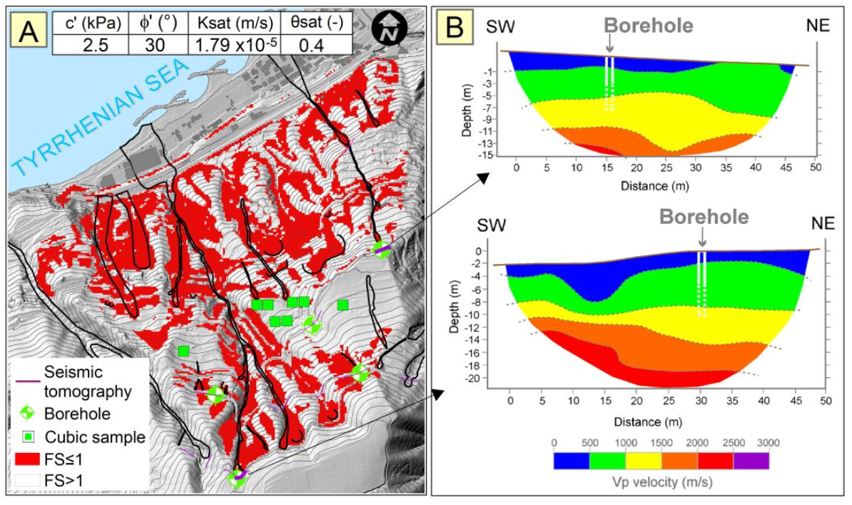
The best landslide susceptibility map (Figure 2A) was obtained considering the average values of hydraulic parameters (Ksat = 1.79 × 10⁻⁵ m/s, saturated hydraulic diffusivity D0 = 7.92 × 10⁻⁵ m2/s and θsat = 0.4) and a constant value of the soil cover thickness equal to 1.5 m [11]. With reference to the shear strength parameters, a value of intercept cohesion equal to 2.5 kPa and a value of the angle of shear strength equal to 30° were used.
According to the above map (Figure 2A), in phase II, in situ investigations were first located in the most susceptible areas identified in phase I and later performed with the general intent to gather useful information to characterise in-depth the soils potentially involved in shallow landslides from a geotechnical point of view in either saturated or unsaturated soil conditions. The in situ investigations consisted of seismic refraction tomographies and boreholes including sampling; on the other hand, the locations where the sampling of cubic samples had to be carried out were established according to logistic reasons (Figure 2A).
Seismic refraction tomographies and boreholes allowed us to determine the thickness of soil covers (gneiss of weathering class VI) potentially involved in the shallow landsliding. The gathered information showed that the thickness value is less than 2 m, being in most cases equal to 1.5 m. The results of the two seismic refraction tomographies, validated by the boreholes’ results, are shown in Figure 2B.
Undisturbed samples taken along the boreholes along with the cubic samples were used to perform several geotechnical laboratory tests to classify and (hydraulically and mechanically) characterise the residual, colluvial and detrital soils (of weathering class VI).
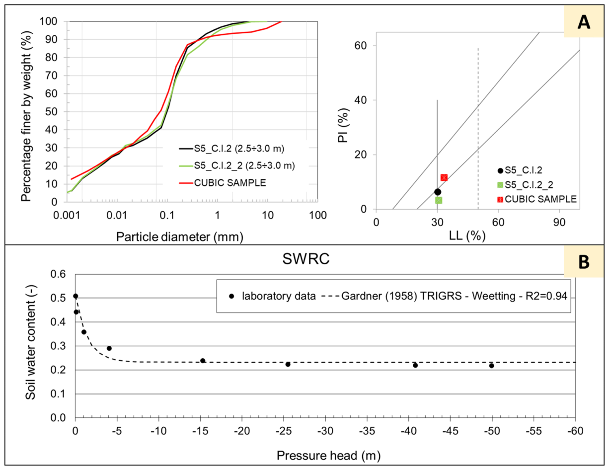
Based on the grain-size distribution and according to the Unified Soil Classification System (USCS), the above soils were classified as well-sorted silty sand (SM) and clayey sand (SC) with an inorganic fine fraction of medium compressibility and not active. The liquid limit (LL) values ranged from 30.2% to 33.4%, whereas those pertained to the plasticity index (PI) from 3.2% to 11.4% (Figure 3A). The solid unit weight (γs) varied from 25.9 kN/m3 to 26.1 kN/m3, the void ratio (e) ranged from 0.9 to 1.17, and the porosity (n) varied from 47% to 54%.
As for the hydraulic properties, permeability tests were performed in an oedometer apparatus at different consolidation stresses equalling 50 kPa, 98.45 kPa, 98.59 kPa, and 196.45 kPa; the corresponding values of the hydraulic conductivity in saturated soil conditions equalled 3.64 × 10⁻⁷ m/s, 1.63 × 10⁻⁸ m/s, 3.97 × 10⁻⁷ m/s and 1.84 × 10⁻⁸ m/s.
The soil water characteristic curve was obtained by means of a suction-controlled oedometer test, and the laboratory data were fitted with the Gardner model for obtaining an R-squared value equalling 0.94 (Figure 3B).
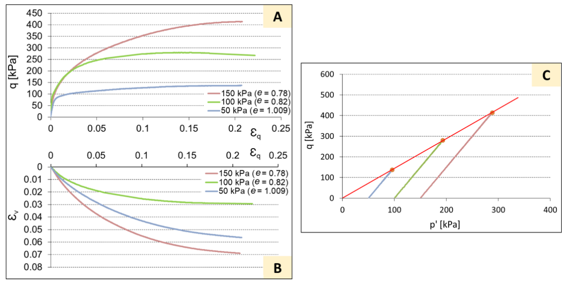
With reference to mechanical properties, the results of drained triaxial compression on undisturbed soil specimens were used to generate the soil strength envelope in saturated soil conditions. These results were represented on the q–εq and εv–εq planes (Figure 4A,B) and on the q–p’ plane (Figure 4C), where q is the deviatoric stress, p’ is the isotropic effective stress, εq is the deviatoric strain, and εv is the volumetric strain. The curves highlight a ductile and contracting behaviour. The obtained shear strength parameters were equal to c′ = 1 kPa and ϕ′ = 35°.
3.2. TRIGRS Analyses
In phase II, the TRIGRS analyses were performed considering soils in saturated and unsaturated conditions.
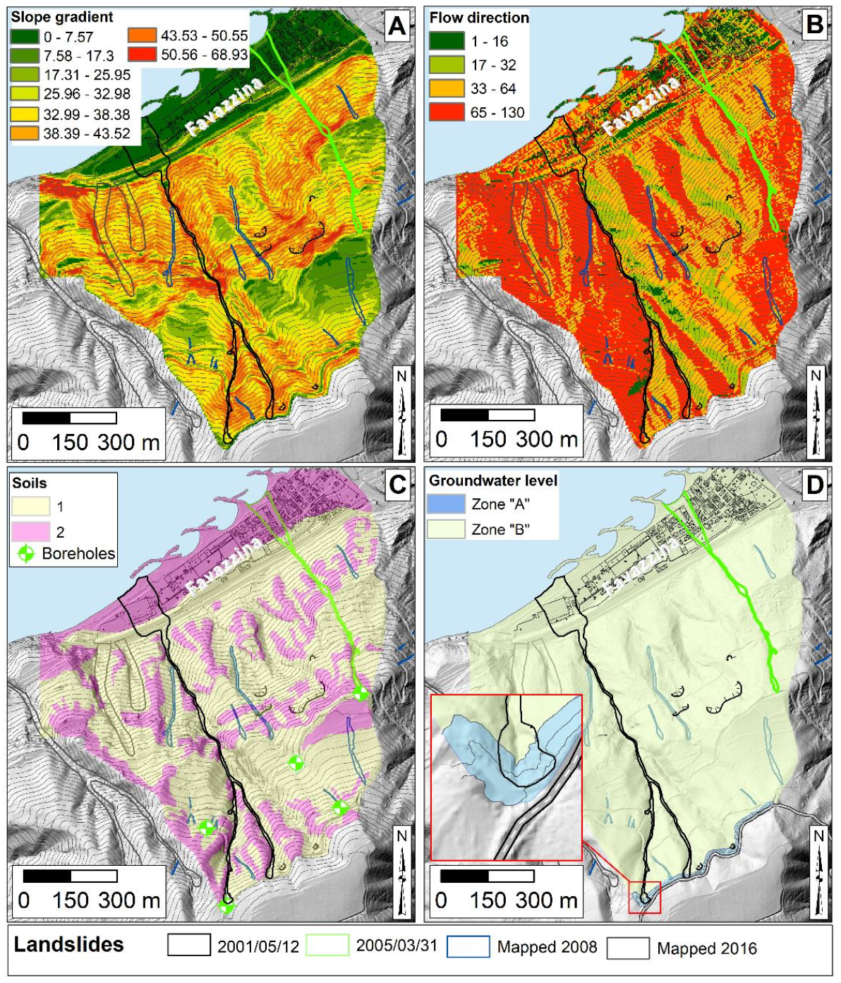
The input data included the DEM (5 m × 5 m), the derived slope gradient map, the flow direction map, the map of the weathered gneiss and the initial depth of the groundwater table (Figure 5). The flow direction map (Figure 5B) was obtained by generating a raster of the flow direction from each cell to its steepest downslope neighbor. The map of the weathered gneiss included two main lithologies (Figure 5C) as follows: (i) SOIL 1, the gneiss of weathering class VI; and (ii) SOIL 2, the gneiss of others weathering classes not potentially involved in the occurrence of shallow landslides.
As for the initial depth of the groundwater table, due to a lack of data, different positions of the water table were considered for the whole study area. Furthermore, according to [11], to analyse the role played by some road tracks along the upper parts of the slopes on shallow landslide triggering, the study area was partitioned in two zones (zone “A” and zone “B”) each associated with a given initial depth of the groundwater table (Figure 5D). Zone “A” was a buffer zone starting from a road track located near the 2001 shallow landslide source areas, and it was constituted by three contour lines, with each equal to 5 m; zone “B” was the remaining part of the study area (Figure 5D).
The values of the geotechnical parameters of SOIL 1 obtained from the performed laboratory tests are summarized in Table 1.
The first column of Table 1 reports an identification number associated with the letter U or S in the cases of unsaturated or saturated soil conditions, respectively. The second and third columns summarize the values of the intercept cohesion and the angle of shear strength obtained by geotechnical laboratory tests. The third to seventh columns summarize the values of the hydraulic conductivity in saturated soil conditions, the saturated and residual volumetric water contents and the Gardner’s parameter. In all considered cases, the value of the hydraulic conductivity obtained by oedometer tests with a consolidation stress equalling 50 kPa was used due to the expected (shallow) depths of the landslides under consideration. The last three columns summarize the values of soil cover thickness (H) and the locations of the initial depth of the groundwater table (zones “A” and “B”).
With reference to the soil cover thickness, a value equal to 1.5 m for the whole study area was considered, because the shear failure surfaces of shallow landslides developed at an average depth of 1.5 m from the ground surface, as confirmed by the in situ investigations.
The saturated hydraulic diffusivity (D0) was calculated according to [31,32] using the equation:
where Sy is the specific yield that was assumed equal to 0.34 according to [33,34], for the considered soils.
Boundary conditions were the same as those adopted in phase I.
Saturated soil conditions were first investigated assumed in zone “A” (Figure 5D), i.e., an initial depth of the groundwater table was set at 1.5 m (with a capillary rise involving the soil thickness on the whole) or 0 m from the topographic surface. In zone “B” (Figure 5D), the initial depth of the groundwater table was keep fixed at 1.5 m (i.e., at the bedrock–soil interface) from the topographic surface.
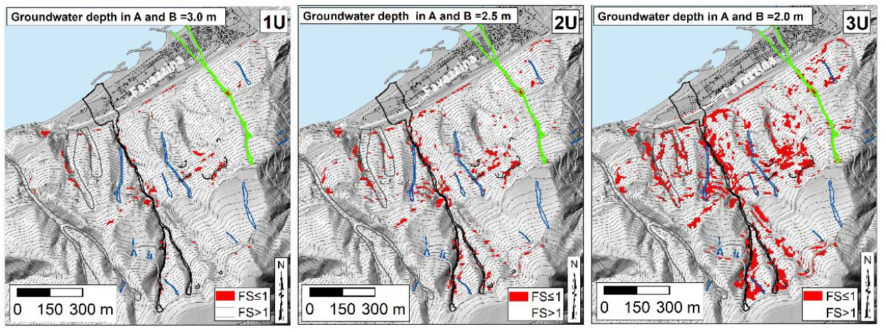
The numerical simulation performed in unsaturated soil conditions with an initial depth of the groundwater table of 3.0 m from the topographic surface (Figure 6, case 1U) showed that only some cells of the study area resulted “unstable”, and therefore, this initial condition did not allow us to match the source areas mapped in the landslide inventory.
If the position of the initial depth of the groundwater table rose, i.e., in the cases when it was located at 2.5 m and 2.0 m from the topographic surface (Figure 6, cases 2U and 3U), the number of cells that resulted “unstable” tended to increase, but with a very limited gain with respect to that in the previous case 1U. Indeed, as Table 2 shows, in these cases 1U and 2U, the values of TPR equalled 0.08 and 0.14, respectively. On the other hand, in the case 3U, the value of TPR equalled 0.45.
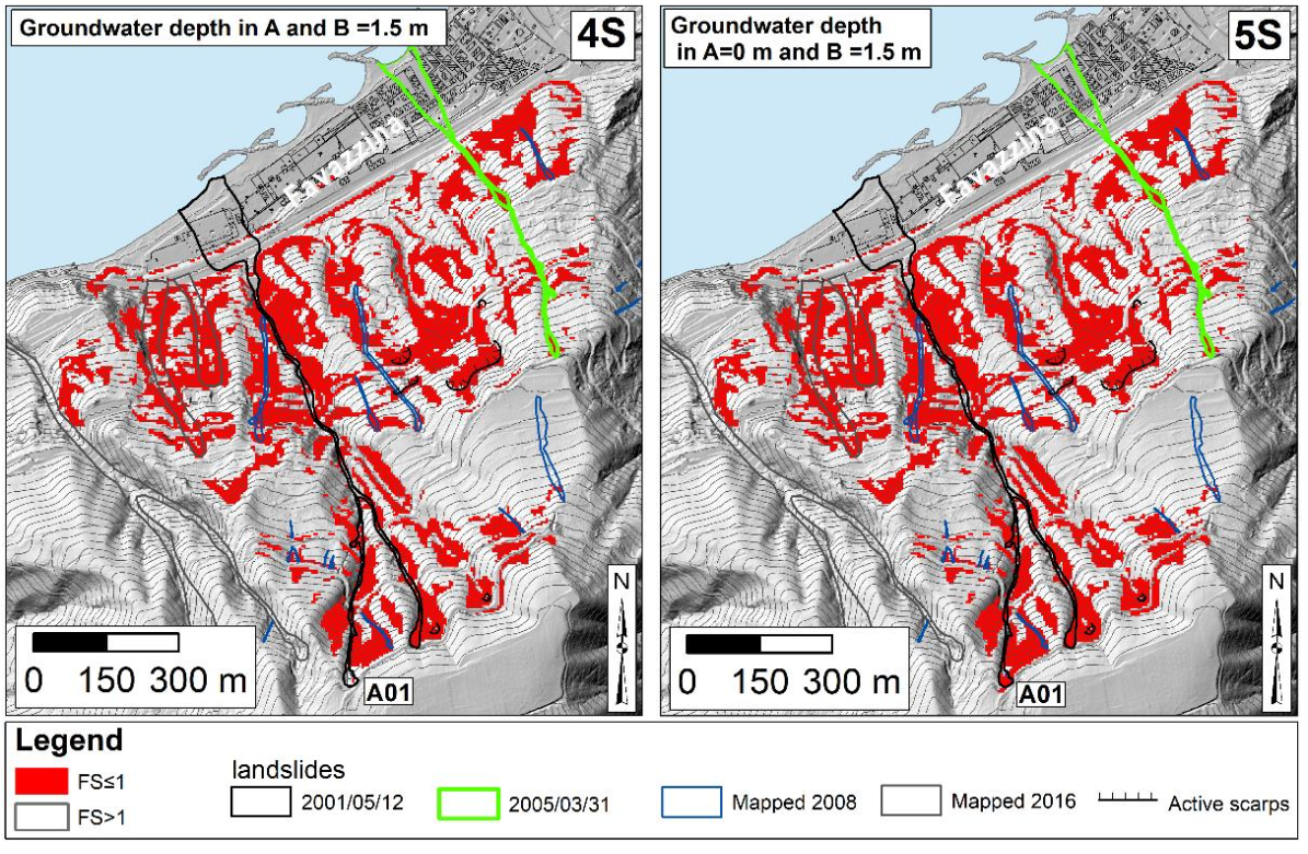
In saturated soil conditions, the TRIGRS results associated with the case 4S in Table 1 (Figure 7, case 4S) showed that the areas computed as “unstable” well matched the source areas mapped in the landslide inventory, except the area A01 that was among the ones related to the 2001 event. On the contrary, considering the case 5S in Table 1 (Figure 7, case 5S), it can be observed that TRIGRS allowed for correctly back-analysing the source areas mapped in the landslide inventory including A01.
Table 2 highlights how the highest TPR values pertained just to TRIGRS analyses carried out in saturated soil conditions. Particularly, the TPR attained values equalling 0.84 in the case 4S and 0.86 in the case 5S.
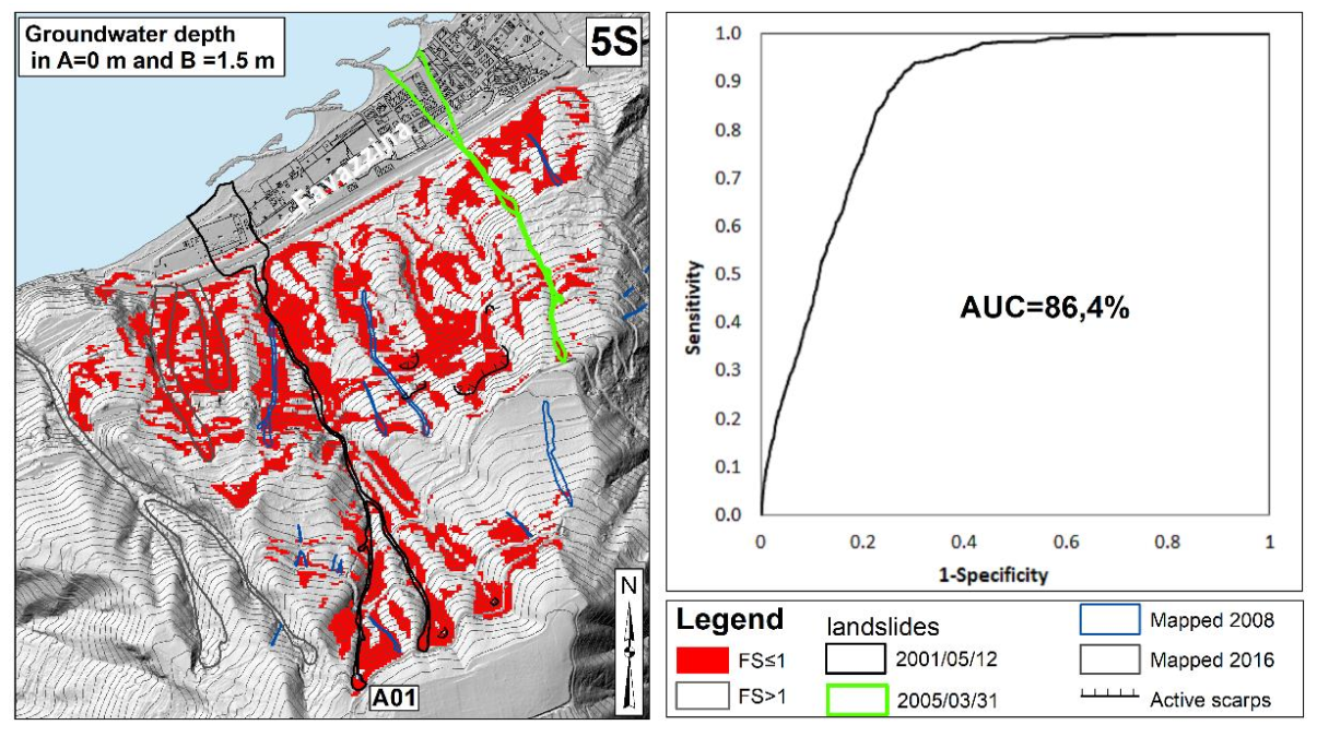
For case 5S, the AUC was also estimated to confirm the success of the TRIGRS analysis. In this regard, Figure 8 shows that the value of the area under the ROC curve plotted in the sensitivity versus 1-the specificity space was equal to 86.4%.
4. Discussion and Conclusions
The results obtained in this work with reference to a case study in the Calabria region (southern Italy) demonstrated that the TRIGRS model can allow for both guiding in properly locating in situ investigations that include sampling and forecasting shallow landslide source areas, once a reliable geotechnical slope model is defined according to laboratory test results. The achievement of these goals was facilitated by the limited extent of the study area and by the involvement of gneiss (in source areas) similar to the genesis and the weathering grade (class VI). Moreover, the role played by a given initial condition, i.e., the initial depth of the groundwater table from the topographic surface, on the stability of slopes was highlighted. Particularly, the work hypothesis on saturated soil conditions led to results that well matched the source areas of past events, especially if the initial groundwater table coincided with the topographic surface in the zone of the slope where the existence of road tracks was recognised (case 5S). This is not the case of soils in unsaturated (initial) conditions. On the other hand, the capability of the TRIGRS model to provide good predictions of shallow landslides that might occur in the future was testified by an AUC value of the ROC curve exceeding the 80% for the same case 5S, despite the use of a single set of parameter values for the weathered gneiss involved in source areas. Further refinements of the results could be achieved by increasing the number of both in situ investigations and laboratory tests useful to reconstruct the spatial variability of both hydraulic and mechanical properties of the aforementioned weathered gneiss. This would allow passing from the adoption of a deterministic method to a probabilistic one [4,5,6].
Referring to the initial water table, the choice to sub-divide the study area into two zones with different values of the initial depth of the groundwater table is in agreement with the scientific literature on the topic, mainly if road tracks can act as preferential paths of water flow leading to the localised increases of the pore water pressures [11,12,21].
The role played by the rainfall in the triggering of shallow landslides in the study area requires further investigations. Indeed, rainfall data used in TRIGRS analyses carried out in this work were gathered from the only available rain gauge station located at the lowest elevations, along the coast not so far from the study area. The latter showed local rain conditions that hardly can be recorded by that rain gauge station. In this regard, a wider monitoring system including a rain gauge, a thermometer, a wind gauge, several tensiometers and piezometers at different depths from the topographic surface is being installed to control the variability of the weather conditions in the area potentially affected by shallow landslides and the related hydraulic effects on the ground.
The data recorded by the newly installed instrumentation monitoring will fill the gap associated with an unknown position of the initial depth of the groundwater table for improving the performance of the used physically based model.
Author Contributions
Conceptualization, N.M., M.C.M. and M.C.; methodology, N.M., M.C.M. and M.C.; formal analysis, N.M., M.C.M. and M.C.; investigation and laboratory tests, M.C.M., M.C., V.F. and S.F.; resources, N.M., M.C.M. and M.C.; data curation, N.M., M.C.M. and M.C.; writing—original draft preparation, M.C.M. and M.C.; writing—review and editing, N.M., S.F., M.C.M. and M.C.; supervision, N.M. and M.C.M.; project administration, N.M.; funding acquisition, N.M. All authors have read and agreed to the published version of the manuscript.
Funding
This research was funded by the Italian Ministry of University and Research, the National Operative Project number PON ARS01_00158 (Temi Mirati). Specialization area: Smart Secure and Inclusive Communities, estimated cost of 6,788,920.00 euros.
Institutional Review Board Statement
Not applicable.
Informed Consent Statement
Not applicable.
Data Availability Statement
The data presented in this study are available within the manuscript.
Conflicts of Interest
The authors declare no conflict of interest.
References
- Fell, R.; Ho, K.K.S.; Lacasse, S.; Leroi, E. A framework for landslide risk assessment and management. In Landslide Risk Management; CRC Press: Boca Raton, FL, USA, 2005; pp. 13–36. [Google Scholar]
- Fell, R.; Corominas, J.; Bonnard, C.; Cascini, L.; Leroi, E.; Savage, W.Z. Guidelines for landslide susceptibility, hazard and risk zoning for land use planning. Eng. Geol. 2008, 102, 85–98. [Google Scholar] [CrossRef] [Green Version]
- Corominas, J.; van Westen, C.; Frattini, P.; Cascini, L.; Malet, J.P.; Fotopoulou, S.; Catani, F.; Van Den Eeckhaut, M.; Mavrouli, O.; Agliardi, F.; et al. Recommendations for the quantitative analysis of landslide risk. Bull. Eng. Geol. Environ. 2014, 73, 209–263. [Google Scholar] [CrossRef]
- Volpe, E.; Ciabatta, L.; Salciarini, D.; Camici, S.; Cattoni, E.; Brocca, L. The impact of probability density functions assessment on model performance for slope stability analysis. Geosciences 2021, 11, 322. [Google Scholar] [CrossRef]
- Salciarini, D.; Fanelli, G.; Tamagnini, C. A probabilistic model for rainfall-induced shallow landslide prediction at the regional scale. Landslides 2017, 14, 1731–1746. [Google Scholar] [CrossRef]
- Salciarini, D.; Volpe, E.; Cattoni, E. Probabilistic vs. deterministic approach in landslide triggering prediction at large–scale. In Proceedings of the National Conference of The Researchers of Geotechnical Engineering, Istanbul, Turkey, 16–17 May 2019; Springer: Berlin, Germany, 2009; pp. 62–70. [Google Scholar]
- Mandaglio, M.C.; Moraci, N.; Gioffrè, D.; Pitasi, A. Susceptibility analysis of rapid flowslides in southern Italy. In Proceedings of the IOP Conference Series: Earth and Environmental Science, Warwick, UK, 10–11 September 2015; 2015; Volume 26. [Google Scholar]
- Mandaglio, M.C.; Gioffrè, D.; Pitasi, A.; Moraci, N. Qualitative landslide susceptibility assessment in small areas. Procedia Eng. 2016, 158, 440–445. [Google Scholar] [CrossRef] [Green Version]
- Mandaglio, M.C.; Moraci, N.; Gioffrè, D.; Pitasi, A. A procedure to evaluate the susceptibility of rapid flowslides in Southern Italy. In Landslides and Enginered Slopes. Experience, Theory and Practice; CRC Press: Boca Raton, FL, USA, 2018; pp. 1339–1344. [Google Scholar]
- Ciurleo, M.; Mandaglio, M.C.; Moraci, N.; Pitasi, A. A method to evaluate debris flow triggering and propagation by numerical analyses. Lect. Notes Civ. Eng. 2020, 40, 33–41. [Google Scholar] [CrossRef]
- Ciurleo, M.; Mandaglio, M.C.; Moraci, N. Landslide susceptibility assessment by TRIGRS in a frequently affected shallow instability area. Landslides 2019, 16, 175–188. [Google Scholar] [CrossRef]
- Ciurleo, M.; Mandaglio, M.C.; Moraci, N. A quantitative approach for debris flow inception and propagation analysis in the lead up to risk management. Landslides 2021, 18, 2073–2093. [Google Scholar] [CrossRef]
- Borrelli, L.; Critelli, S.; Gullà, G.; Muto, F. Weathering grade and geotectonics of the western-central Mucone River basin (Calabria, Italy). J. Maps 2014, 11, 606–624. [Google Scholar] [CrossRef]
- Borrelli, L.; Coniglio, S.; Critelli, S.; La Barbera, A.; Gullà, G. Weathering grade in granitoid rocks: The San Giovanni in Fiore area (Calabria, Italy). J. Maps 2015, 12, 260–275. [Google Scholar] [CrossRef] [Green Version]
- Gullà, G.; Mandaglio, M.C.; Moraci, N. Effect of weathering on the compressibility and shear strength of a natural clay. Can. Geotech. J. 2011, 43, 618–625. [Google Scholar] [CrossRef]
- Gullà, G.; Moraci, N.; Mandaglio, M.C. Influence of Degradation Cycles on the Mechanical Characteristics of Natural Clays|ISSMGE. Available online: https://www.issmge.org/publications/publication/influence-of-degradation-cycles-on-the-mechanical-characteristics-of-natural-clays (accessed on 6 December 2021).
- Frattini, P.; Crosta, G.; Carrara, A. Techniques for evaluating the performance of landslide susceptibility models. Eng. Geol. 2010, 111, 62–72. [Google Scholar] [CrossRef]
- Borrelli, L.; Gioffrè, D.; Gullà, G.; Moraci, N. Suscettibilità alle frane superficiali e veloci in terreni di alterazione: Un possibile contributo della modellazione della propagazione. Rend. Online Soc. Geol. Ital. 2012, 21, 534–536. [Google Scholar]
- Gioffrè, D.; Moraci, N.; Borrelli, L.; Gullà, G. Numerical code calibration for the back analysis of debris flow runout in southern Italy. In Landslides and Engineered Slopes. Experience, Theory and Practice; CRC Press: Boca Raton, FL, USA, 2016; Volume 2, pp. 991–997. [Google Scholar]
- Bonavina, M.; Bozzano, F.; Martino, S.; Pellegrino, A.; Prestininzi, A.; Scandurra, R. Le colate di fango e detrito lungo il versante costiero tra Bagnara Calabra e Scilla (Reggio Calabria): Valutazioni di suscettibilità. G. Geol. Appl. 2 2005, 2, 65–74. [Google Scholar] [CrossRef]
- LOTTO 05—Attività di Monitoraggio di Siti in Frana e di Aree Soggette a Fenomeni di Subsidenza Rel. Fin. ALLEGATI. Available online: https://docplayer.it/8830116-Lotto-05-attivita-di-monitoraggio-di-siti-in-frana-e-di-aree-soggette-a-fenomeni-di-subsidenza-rel-fin-allegati.html (accessed on 6 December 2021).
- Moraci, N.; Mandaglio, M.C.; Gioffrè, D.; Pitasi, A. Debris flow susceptibility zoning: An approach applied to a study area. Riv. Ital. Geotec. 2017, 51, 47–62. [Google Scholar] [CrossRef]
- Taylor, D.W. Fundamentals of Soil Mechanics; Williams & Wilkins: Philadelphia, PA, USA, 1948. [Google Scholar]
- Bishop, A. The Principle of Effective Stress. Tek. Ukebl. 1959, 106, 859–863. [Google Scholar]
- Vanapalli, S.K.; Fredlund, D.G. Comparison of different procedures to predict unsaturated soil shear strength. Adv. Unsatur. Geotech. 2000, 287, 195–209. [Google Scholar] [CrossRef] [Green Version]
- Gardner, W.R. Some steady-state solutions of the unsaturated moisture flow equation with application to evaporation from a water table. Soil Sci. 1958, 85, 228–232. [Google Scholar] [CrossRef]
- Baum, R.L.; Savage, W.Z.; Godt, J.W. TRIGRS—A Fortran Program for Transient Rainfall Infiltration and Grid-Based Regional Slope-Stability Analysis, Version 2.0; U.S. Geological Survey: Reston, VA, USA, 2008.
- Salciarini, D.; Godt, J.W.; Savage, W.Z.; Conversini, P.; Baum, R.L.; Michael, J.A. Modeling regional initiation of rainfall-induced shallow landslides in the eastern Umbria Region of central Italy. Landslides 2006, 3, 181–194. [Google Scholar] [CrossRef]
- Sorbino, G.; Sica, C.; Cascini, L. Susceptibility analysis of shallow landslides source areas using physically based models. Nat. Hazards 2010, 53, 313–332. [Google Scholar] [CrossRef]
- Swets, J.A. Measuring the accuracy of diagnostic systems. Science 1988, 240, 1285–1293. [Google Scholar] [CrossRef] [Green Version]
- Grelle, G.; Soriano, M.; Revellino, P.; Guerriero, L.; Anderson, M.G.; Diambra, A.; Fiorillo, F.; Esposito, L.; Diodato, N.; Guadagno, F.M. Space-time prediction of rainfall-induced shallow landslides through a combined probabilistic/deterministic approach, optimized for initial water table conditions. Bull. Eng. Geol. Environ. 2018, 73, 877–890. [Google Scholar] [CrossRef]
- Schilirò, L.; Esposito, C.; Scarascia Mugnozza, G. Evaluation of shallow landslide-triggering scenarios through a physically based approach: An example of application in the southern Messina area (northeastern Sicily, Italy). Nat. Hazards Earth Syst. Sci. 2015, 15, 2091–2109. [Google Scholar] [CrossRef] [Green Version]
- Johnson, A.I. Specific Yield Compilation of Specific Yields for Various Materials. Water Supply Paper 1662-D; US Geological Survey: Washington, DC, USA, 1967. [CrossRef]
- Loheide, S.P.; Butler, J.J.; Gorelick, S.M. Estimation of groundwater consumption by phreatophytes using diurnal water table fluctuations: A saturated-unsaturated flow assessment. Water Resour. Res. 2005, 41, 1–14. [Google Scholar] [CrossRef]
Figure 1.
(A) geographical location of the study area; (B) weathering-grade map and multitemporal landslide inventory of the study area (modified from [11]). Weathering-grade map legend: (1) gneiss of class II; (2) gneiss of class III; (3) gneiss of class IV; (4) gneiss of class V; (5) gneiss of class VI; (6) coastal and alluvial deposits; (7) terraced marine deposits; (8) marine coarse sandstone deposits; (9) landslide debris.

Figure 2.
(A) Map used to locate in situ investigations; (B) results of some boreholes and seismic refraction tomographies (vp represents the primary wave velocity).
Figure 2.
(A) Map used to locate in situ investigations; (B) results of some boreholes and seismic refraction tomographies (vp represents the primary wave velocity).

Figure 3.
Results of laboratory tests on weathered gneiss of class VI. (A) Grain size distribution and plasticity chart; (B) soil-water retention curve (SWRC).
Figure 3.
Results of laboratory tests on weathered gneiss of class VI. (A) Grain size distribution and plasticity chart; (B) soil-water retention curve (SWRC).

Figure 4.
(A) Results of the drained triaxial compression on specimens of gneiss of weathering class VI on the q–εq plane. (B) Results of the drained triaxial compression on specimens of gneiss of weathering class VI on the εv–εq plane (e represents the void ratio of specimens). (C) Stress paths and failure envelope.

Figure 5.
Transient Rainfall Infiltration and Grid-based Slope-Stability (TRIGRS) input data: (A) slope gradient (°) map; (B) flow direction map; (C) map of weathered gneiss; (D) map of zones with given values of the initial depth of the groundwater table. In the red box, there is an enlarged area showing the three contour lines, with each equal to 5 m and used to individuate zone “A”.

Figure 6.
TRIGRS results in unsaturated soil conditions for cases 1U, 2U and 3U.

Figure 7.
TRIGRS results in saturated soil conditions for cases 4S and 5S.

Figure 8.
The best result obtained by the TRIGRS model in terms of the true positive rate (TPR) and the area under the receiver-operating characteristic curve (AUC) (case 5S).
Figure 8.
The best result obtained by the TRIGRS model in terms of the true positive rate (TPR) and the area under the receiver-operating characteristic curve (AUC) (case 5S).


Table 1.
Input data used in the TRIGRS under saturated and unsaturated soil conditions.
| CASE | c′ (kPa) | Φ′ (°) | Ksat (m/s) | Θs (-) | Θr (-) | α (m−1) | H (m) | Initial Depth of the Groundwater Table in Zone “A” (m) | Initial Depth of the Groundwater Table in Zone “B”(m) |
|---|---|---|---|---|---|---|---|---|---|
| 1U | 1 | 35 | 3.64 × 10⁻⁷ | 0.51 | 0.23 | 0.69 | 1.5 | 3.0 | 3.0 |
| 2U | 1 | 35 | 3.64 × 10⁻⁷ | 0.51 | 0.23 | 0.69 | 1.5 | 2.5 | 2.5 |
| 3U | 1 | 35 | 3.64 × 10⁻⁷ | 0.51 | 0.23 | 0.69 | 1.5 | 2.0 | 2.0 |
| 4S | 1 | 35 | 3.64 × 10⁻⁷ | 0.51 | 0.23 | - | 1.5 | 1.5 | 1.5 |
| 5S | 1 | 35 | 3.64 × 10⁻⁷ | 0.51 | 0.23 | - | 1.5 | 0 | 1.5 |
Table 2.
Contingency table.
| Case | TP | FN | FP | TN | TPR | FPR |
|---|---|---|---|---|---|---|
| 1U | 70 | 846 | 479 | 38,389 | 0.08 | 0.01 |
| 2U | 161 | 755 | 1424 | 37,444 | 0.18 | 0.04 |
| 3U | 411 | 505 | 4216 | 34,652 | 0.45 | 0.11 |
| 4S | 766 | 150 | 9350 | 29,518 | 0.84 | 0.24 |
| 5S | 787 | 129 | 9454 | 29,414 | 0.86 | 0.24 |
Publisher’s Note: MDPI stays neutral with regard to jurisdictional claims in published maps and institutional affiliations. |
© 2021 by the authors. Licensee MDPI, Basel, Switzerland. This article is an open access article distributed under the terms and conditions of the Creative Commons Attribution (CC BY) license (https://creativecommons.org/licenses/by/4.0/).
Share and Cite
MDPI and ACS Style
Ciurleo, M.; Ferlisi, S.; Foresta, V.; Mandaglio, M.C.; Moraci, N. Landslide Susceptibility Analysis by Applying TRIGRS to a Reliable Geotechnical Slope Model. Geosciences 2022, 12, 18. https://doi.org/10.3390/geosciences12010018
AMA Style
Ciurleo M, Ferlisi S, Foresta V, Mandaglio MC, Moraci N. Landslide Susceptibility Analysis by Applying TRIGRS to a Reliable Geotechnical Slope Model. Geosciences. 2022; 12(1):18. https://doi.org/10.3390/geosciences12010018
Chicago/Turabian StyleCiurleo, Mariantonietta, Settimio Ferlisi, Vito Foresta, Maria Clorinda Mandaglio, and Nicola Moraci. 2022. "Landslide Susceptibility Analysis by Applying TRIGRS to a Reliable Geotechnical Slope Model" Geosciences 12, no. 1: 18. https://doi.org/10.3390/geosciences12010018
Note that from the first issue of 2016, this journal uses article numbers instead of page numbers. See further details here.