


Seafloor and Ocean Crust Structure of the Kerguelen Plateau from Marine Geophysical and Satellite Altimetry Datasets


Laboratory of Image Synthesis and Analysis, École polytechnique de Bruxelles, Université Libre de Bruxelles (ULB), Building L, Campus du Solbosch, ULB—LISA CP165/57, Avenue Franklin D. Roosevelt 50, 1050 Brussels, Belgium
Geomatics 2023, 3(3), 393-426; https://doi.org/10.3390/geomatics3030022
Submission received: 11 July 2023
/
Revised: 6 August 2023
/
Accepted: 8 August 2023
/
Published: 10 August 2023
(This article belongs to the Special Issue Advances in Ocean Mapping and Nautical Cartography)
Abstract
:The volcanic Kerguelen Islands are formed on one of the world’s largest submarine plateaus. Located in the remote segment of the southern Indian Ocean close to Antarctica, the Kerguelen Plateau is notable for a complex tectonic origin and geologic formation related to the Cretaceous history of the continents. This is reflected in the varying age of the oceanic crust adjacent to the plateau and the highly heterogeneous bathymetry of the Kerguelen Plateau, with seafloor structure differing for the southern and northern segments. Remote sensing data derived from marine gravity and satellite radar altimetry surveys serve as an important source of information for mapping complex seafloor features. This study incorporates geospatial information from NOAA, EMAG2, WDMAM, ETOPO1, and EGM96 datasets to refine the extent and distribution of the extracted seafloor features. The cartographic joint analysis of topography, magnetic anomalies, tectonic and gravity grids is based on the integrated mapping performed using the Generic Mapping Tools (GMT) programming suite. Mapping of the submerged features (Broken Ridge, Crozet Islands, seafloor fabric, orientation, and frequency of magnetic anomalies) enables analysis of their correspondence with free-air gravity and magnetic anomalies, geodynamic setting, and seabed structure in the southwest Indian Ocean. The results show that integrating the datasets using advanced cartographic scripting language improves identification and visualization of the seabed objects. The results include 11 new maps of the region covering the Kerguelen Plateau and southwest Indian Ocean. This study contributes to increasing the knowledge of the seafloor structure in the French Southern and Antarctic Lands.
Keywords:
Antarctic; Southern Ocean; bathymetry; French Southern and Antarctic Lands; cartography; satellite altimetry; marine geophysics; sediments; magnetic anomalies; seafloorPACS:
91.10.Da; 91.10.Op; 93.85.Pq; 91.10.Fc; 91.10.Jf; 91.10.VrMSC:
86A30; 86-05; 86A04; 86A70JEL Classification:
Y91; C83; C88; C90; C00; C60; C611. Introduction
1.1. Background
In cartography and spatial data processing, the task of plotting maps (also known as mapping layouts) is widely used as a common practice. This involves the visualization and representation of spatially defined objects using cartographic techniques [1,2,3]. One of the generally accepted methods for mapping and quantitative and qualitative cartographic visualization is implemented through Geographic Information Systems (GIS), using algorithms for raster and vector data processing embedded within these programs [4,5,6]. However, the high complexity and time-consuming nature of GIS are not conducive to large-scale mapping applications in various Earth science tasks. To address this, programming and scripting algorithms are proposed as an alternative to the GIS-based approach, aiming to reduce data processing complexity in computer graphics and time costs associated with mapping [7].
The application of programming methods in cartography has seen extensive development, resulting in the release of several programs that utilize scripts as mapping tools. Programming-based cartographic approaches can be categorized into three general types. First, there are partial uses of scripts, such as plugins or alternative tools in addition to the existing Graphical User Interface (GUI) in classical modes. Examples include ESRI’s ModelBuilder [8], modules in the Geographic Resources Analysis Support System (GRASS GIS), processing script editors in QGIS or ArcGIS [9,10], and the Python-based ERDAS Macro Language (EML) used in Erdas Imagine to create spatial models. Second, there are spatial libraries of programming languages, including selected packages in R and Python specifically designed for satellite image processing and geospatial data analysis [11,12,13,14]. Third, there are programs that are completely based on using scripting languages without any Graphical User Interface (GUI), such as the Generic Mapping Tools (GMT). All these examples of using scripts aim to automate cartographic data processing using advanced scripting tools.
The script-based cartographic programs are founded on the principle of utilizing the syntax of a programming language, which includes a number of key commands and recognizable expressions by the system [15]. Following the rules of the embedded language, it becomes possible to compose scripts for data modeling and cartographic visualization. In contrast to traditional GUI-based GIS methods, cartographic scripts do not directly generate maps. However, they provide a series of commands that encompass crucial information about the map’s appearance, governing specific features on a plotted cartographic layout [16]. In fact, scripts and programming commands used in cartography define the elements present on the map produced by the script during execution. Specifically, it is possible to define key map concepts such as mathematical definitions of the map (projections, resolution, grid, coordinate systems, extent, and scale), design of symbols and legends (colors and object sizes, palettes for continuous fields, and transparency), and exposition of the elements (overlay, topology, generalization) [17].
1.2. Problem Formulation
The analysis of the seafloor structure and ocean crust concerns mapping, detecting, and recognising the bathymetric structures and variations in geophysical fields. Among these problems, the integrated geophysical interpretation of the satellite altimetry, marine gravimetry, and magnetic anomalies, as well as acoustic and seismic surveys present one of the most active research areas that have attracted research interest in recent decades [18]. Previous studies [19] provided a broad overview of approaches for analysis of the satellite gravimetry data to model the Earth beneath the sea. Marine geophysical and satellite altimetry data provide information on crustal density and processes in the upper mantle [20,21,22], sediment thickness and basement depth [23]. Moreover, the analysis of the geophysical data enables to reveal key characteristics regarding the lithosphere thickness such as Moho discontinuity and elastic features of the lithosphere [24], viscosity and flexural rigidity. Such data are essential for investigations on the Earth’s structure.
In terms of the data-driven analyses, previous works investigating the oceanic seabed can be roughly classified into studies focused on the bathymetric mapping and geophysical analysis. Mapping the seafloor characterizes the bathymetric patterns using data visualization and cartographic methods [25,26,27]. Marine geophysical methods investigate the geology of the continental margins using methods of deep-sea drilling [28,29], the analysis of features extracted from seismic survey and remote sensing data [30], investigating the structure of the deep ocean basins [31,32,33], and modelling the mid-ocean ridge system [34,35,36]. Although traditional methods of bathymetric survey supply novel information on origin, evolution, structure, stratigraphy, and tectonic features of the oceanic crust, they require costly hydrographic equipment such as mutlibeam echo sounder systems [37].
1.3. Related Work
Seafloor bathymetry and geophysical setting of the oceanic crust are two important topics for modelling lithosphere [38]. However, the integrated capture and processing of the multi-source data—such as bathymetry, marine geologic data (development on the Earth’s crust including age, spreading rates and symmetry) and marine geophysical data (sediment thickness, gravity and magnetic anomalies)—has always been a challenging task, and few attempts have been made to explore it. Since the variety of data sources is increasing in modern cartography, it results in an exponential growth in the volume of data serving cartographic applications [39]. Therefore, the use of the remote sensing data, satellite altimetry and gravimetry has proven to be effective in geophysical studies. Numerous examples exist in the literature that focus on estimating the geoid values, evaluating gravity anomalies, analysis of the tectonic and crustal structures, glacial and hydrological modelling and habitat mapping.
Satellite altimetry data can be used to jointly represent the patterns of the oceanic currents and to draw conclusions on connectivity between the habitats [40]. For instance, a study by [41] uses the hydrographic and acoustic data for the analysis of the vertical layers of the ocean to identify the community distribution. An example of the tide modelling of bathymetric gradients was presented using the satellite altimetry data [42]. The retreat of glaciers using mass balance measurements was estimated using remote sensing data to analyze spatial distribution of the surface mass balance [43]. Other studies used the Gravity Recovery and Climate Experiment (GRACE) mission for detecting trends and variations in the ice-sheet mass balance by evaluating gravity signals [44]. Furthermore, Mathieu et al. [45] combine the SRTM DEM, remote sensing data and geological sampling to clarify seafloor structures.
These and similar examples illustrate that a combination of bathymetric and geophysical data for the detailed analysis of Earth’s crust structure and topography outperforms their use separately. This suggests that seafloor mapping should be based on the complex analysis of the heterogeneous features of the seabed. Such information can be derived from various Earth observation datasets, as pointed out earlier [46,47,48,49]. Since such methods can be regarded as feature-level combinations of seafloor features showing the local appearance of prominent seabed elements such as fracture zones, ridges, seamounts, deep-sea trenches, canyons, or rifts, the use of a programming approach to merge different integrated geophysical datasets enables matching multi-source data with varying resolutions and origins. Such data can be used for the detailed analysis of seafloor structure and geodynamic processes [50,51,52].
1.4. Objection and Motivation
In this study, several bathymetric and marine geophysical datasets were used for the analysis of the Kerguelen Plateau (Figure 1) within the south-western segment of the Indian Ocean to visualize, describe and analyze the structures of the seafloor in the context of the geophysical settings. Ten new maps are presented and described to visualize spatial variations, reveal correlation and matches between the geophysical and topographic setting of the Kerguelen region to continue the existing similar studies [53,54,55]. Given the remote location of the Kerguelen Archipelago, one of the most isolated places on Earth, and associated difficulties and high cost of geological and geophysical sampling, the integrated use of the satellite-derived data enables to us have better insight into the structure of the Kerguelen Plateau.
2. Study Area
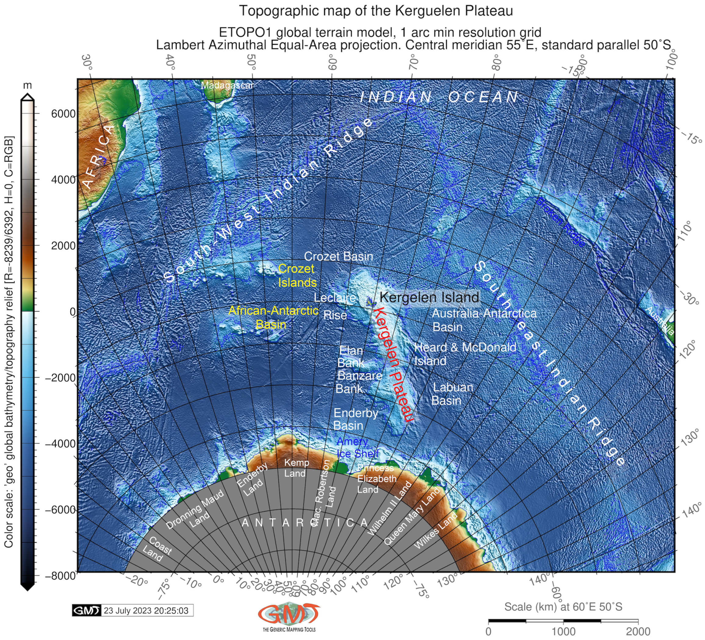
The Kerguelen Plateau presents a large topographic elevation in the south-west Indian Ocean, extending over 6500 km [56], Figure 1. The Kerguelen Archipelago, formed on the plateau, constitutes a shallow submarine plateau. The structure of the Kerguelen Archipelago is asymmetric with notable variations in the two distinct parts: the northern part (Heard, McDonald and Kerguelen Islands) is more shallow (<1000 m) compared to the southern segment (depths of 1500–2000 m) [57]. Morphologically, the plateau is oriented in a NNW direction toward the Antarctic continental margin where it is constrained by Princess Elizabeth Land. On the northwest, the archipelago is limited by the Crozet Archipelago, located 1250 km away [58]. To the north, it is bordered by the African-Antarctic Basins; to the northeast, by the Australian-Antarctic Basin; and to the south, by the Antarctic. Adjacent lands include Enderby Land, Kemp Land, Mac Robertson Land, Princess Elizabeth Land, Wilhelm II Land, and Queen Mary Land, all located in the Antarctic, as shown in Figure 2.
The origin of the Kerguelen Plateau is related to the hotspot associated with the Gondwana breakup in the Cretaceous period (120–110 Ma), and seafloor spreading between India and Antarctica in the south-western Indian Ocean [59]. The initial surface manifestations of the Kerguelen Plume in the southern region began during the Mesozoic era around 120 Ma [60]. Active submarine volcanism occurring on the aseismic ridge, coupled with sedimentation processes since the Cretaceous, led to the creation of the basaltic basement of the Kerguelen region [61]. This volcanic activity persisted within the Kerguelen hotspot until the Tertiary period (<40 Ma) and is evident in the geological and mineralogical composition of the archipelago. The archipelago is covered by up to 85% basalts originating from the mantle plume of the hotspot. These basalts result from the crystallization of raised and cooled basaltic magma [62,63,64]. Presently, the Kerguelen Plateau stands as one of the largest volcanic plateaus globally, spanning a total length of 2300 km. Remnants of volcanic activity are still visible on the Heard and McDonald Islands [65].
The Kerguelen Plateau belongs to the French Southern and Antarctic Lands, known for its protected environment [66,67,68]. Its high environmental value is explained by the unique wildlife structure, which includes vulnerable species. The remote location of the archipelago—4000 km from South Africa and Australia [69,70]—has created ideal conditions for preserving unique flora and fauna of the Kerguelen Archipelago. The presence of rare Antarctic plant species and high biodiversity is closely linked to the soil developed on the basaltic basement and the specific geological substrate of volcanic origin. Additional factors contributing to this uniqueness include the influence of the Polar climate [71,72,73]. The distribution of fish communities and phytoplankton is affected by seasonal changes of the Antarctic circumpolar currents [74,75,76,77,78,79,80,81]. Furthermore, the steep bathymetric slopes and the exposure of the Kerguelen plateau amplify the speed and intensity of the ocean currents’ circulation [82]. The combination of all these factors makes the ecosystems of the Kerguelen Archipelago unique and deserving of protection as an environmental heritage of the French Southern and Antarctic Lands [83,84,85].
3. Materials and Methods
All the maps have been plotted using the scripting toolset Generic Mapping Tools version 6.4.0 [86], https://www.generic-mapping-tools.org/. A key aspect of the GMT algorithms is that they consider each cartographic element by its parameters and add new layers on the map regarding the target location, which can be adjusted using refined flag options in special modules. Thus, a modular scripting approach of GMT distinguishes it from GIS.
3.1. Data
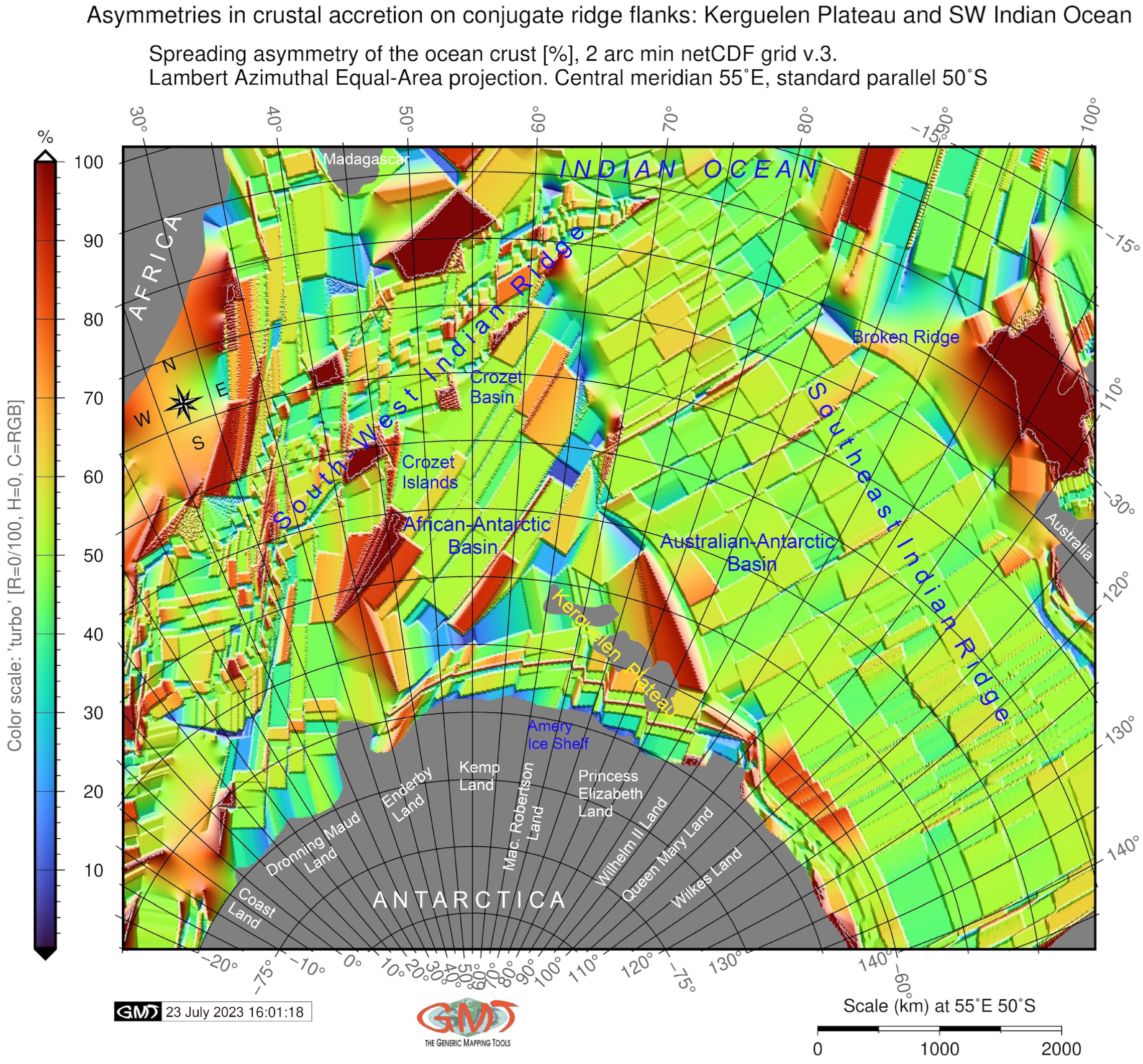
The materials used as input cartographic grids include the following datasets. The marine geological data on age, spreading rates, and asymmetry of the ocean crust were derived from the NOAA high-resolution dataset [87], Figure 3. The units of the dataset on spreading asymmetry are expressed as % of crustal accretion of the seafloor, i.e., symmetric spreading results in values of 50% on conjugate ridge flanks. The bathymetric mapping was based on the ETOPO Global Relief Model [88]. The gravity grids were obtained from the EGM-2008 and EGM96 [89]. Gravity data are grounded on the concept of gravity anomaly across different Earth surfaces, which correlates with the interplay between topography, mass distribution within local and regional relief structures, marine gravity values, and the establishment of gravitational potential across various Earth locations.
The free-air and Bouguer gravity anomaly grids are derived from high-resolution grids [90,91]. Specifically, the gravity field varies significantly over the oceans due to density fluctuations. The most pronounced anomalies emerge from fluctuations in density, such as those occurring at the heterogeneous seafloor or at the crust-mantle interface (Moho discontinuity) [92]. Such data facilitate the modelling of gravity fields for the analysis of Earth’s structure. The latest updates in gravity grids enhance the precision of altimetry-derived gravity anomalies. While gravity grids do not directly indicate topography, they offer crucial insights into the Earth’s relief, providing an approximate relationship between topographic and geophysical data and illustrating the correspondence of surface gravity values with local geoid undulations [93].
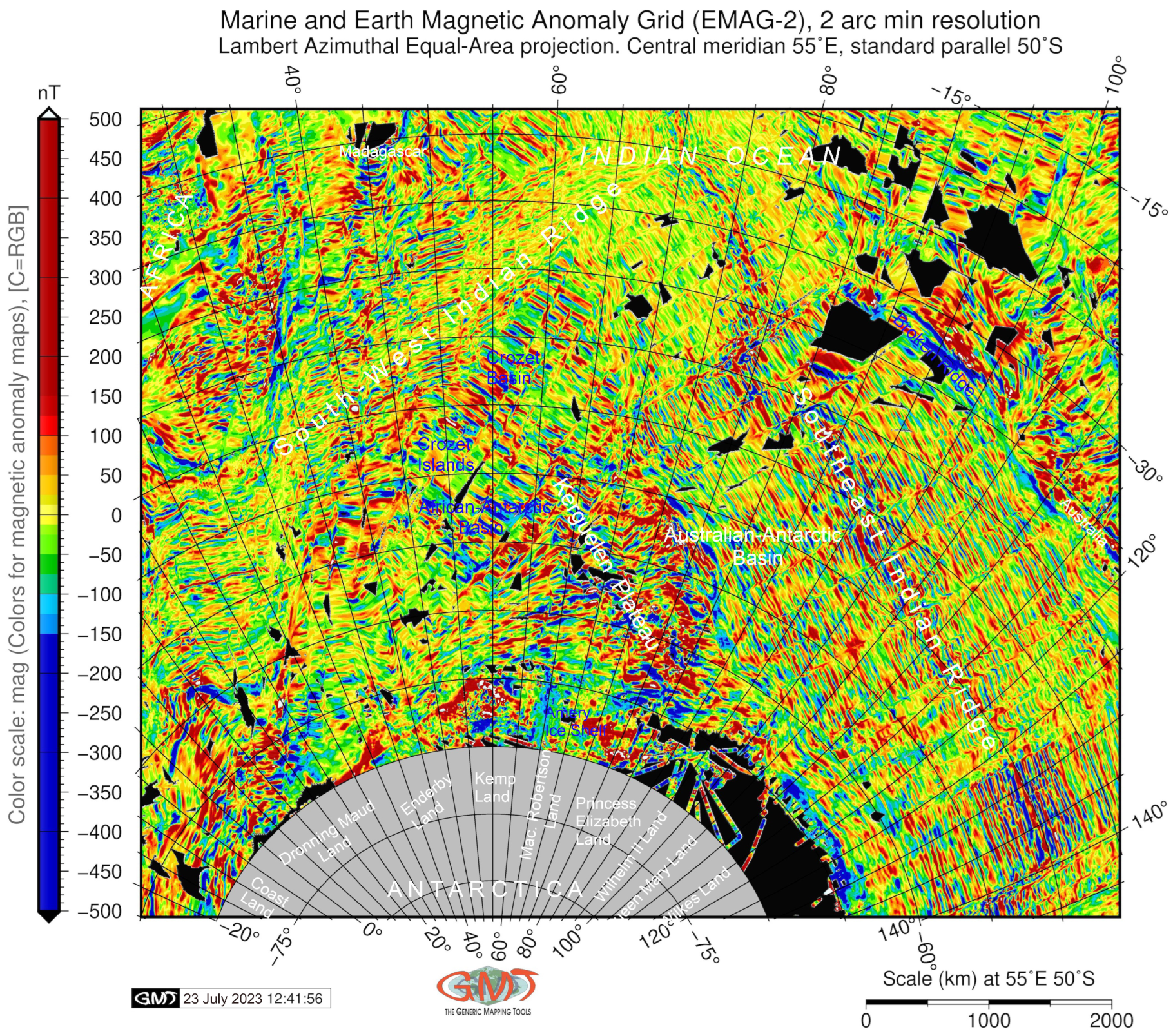
The data on sediment thickness are collected from the GlobSed dataset, which models distribution of the sediment thickness in the World’s Oceans [94]. The magnetic data are derived from the two available information sources compiled originally from satellite and marine magnetic measurements: the Earth Magnetic Anomaly Grid (EMAG2) [95], which has a resolution of two arc minutes, and the World Digital Magnetic Anomaly Map (WDMAM) with a resolution of three minutes [96]. The gravity data were derived from the free-air global gravity grids [97].
The analysis of the geodetic data is useful in such complex terrains since it facilitates the identification of major tectonic structures and topographic patterns. In addition, the EGM grids, the identification of lithospheric structure and tectonic blocks can also be performed using satellite gravity data such as World Gravity Model (WGM) and GRACE [98]. Furthermore, the EGM and astrogeodetic vertical deflections are useful for modelling gravity and geopotential differences [99]. Finally, processing terrestrial and satellite geodetic data can be applied to address theoretical geodetic challenges, such as the altimetry–gravimetry boundary-value problem [100]. Other instances of the implications of geodetic datasets encompass the utilization of satellite-derived data from Cryosat-2 and altimetry in conjunction with ship-measured gravity to estimate marine gravity anomalies [101].
3.2. Methods
In this study, the cartographic methodology is based on using the Generic Mapping Tools (GMT) programming suite version 6.4.0 [102] by the developed scripting workflow, explained in detail in earlier works [103,104]. The most prominent feature of the GMT is a scripting approach that principally distinguishes it from the conventional software due to the embedded programming language [105]. The traditional GIS-based methods either employ the GUI for mapping with existing standard menu or allow scripting as a complimentary workflow.
In contrast, the GMT is a completely console-based software that operates entirely using scripts. In this way, it captures the data by running a script written using the embedded syntax that operates similarly to programming. A script consists of a sequence of predefined commands with parameters that control the appearance of cartographic elements and features. The most well-known cartographic tools that employ scripts for data processing are GMT [106] and GRASS GIS [107]. Other software allows scripts as an additional functionality alongside the standard GUI, as seen in ArcGIS or QGIS. While the latter is predominantly used for image processing, cartographic, and ecological studies [108,109,110,111], GMT finds application in geophysical and geological research [112,113,114].
3.2.1. Topographic/Bathymetric Mapping
The script for plotting the topographic/bathymetric map is provided in Listing A1. The code’s most crucial elements are as follows. The mapping process initiates by selecting the study area from the global ETOPO1 grid using ‘grdcut’. Isolines are chosen through ‘grdcontour’ with a 1,000 m gap. In our case, these lines denote significant locations that offer a high representation estimate for seafloor bathymetry. ‘grdimage’ is utilized to generate an image plot of the raster grid, colored as defined by the ‘makecpt’ module, with values -T indicating the extreme (min/max) data for the topographic grid, as extracted by the ‘gdalinfo’ module. The remaining code details are outlined in Listing A1 along with key comments.
3.2.2. Mapping Seafloor Age, Spreading Rates, Spreading Asymmetry and Age Uncertainty of the Ocean Crust
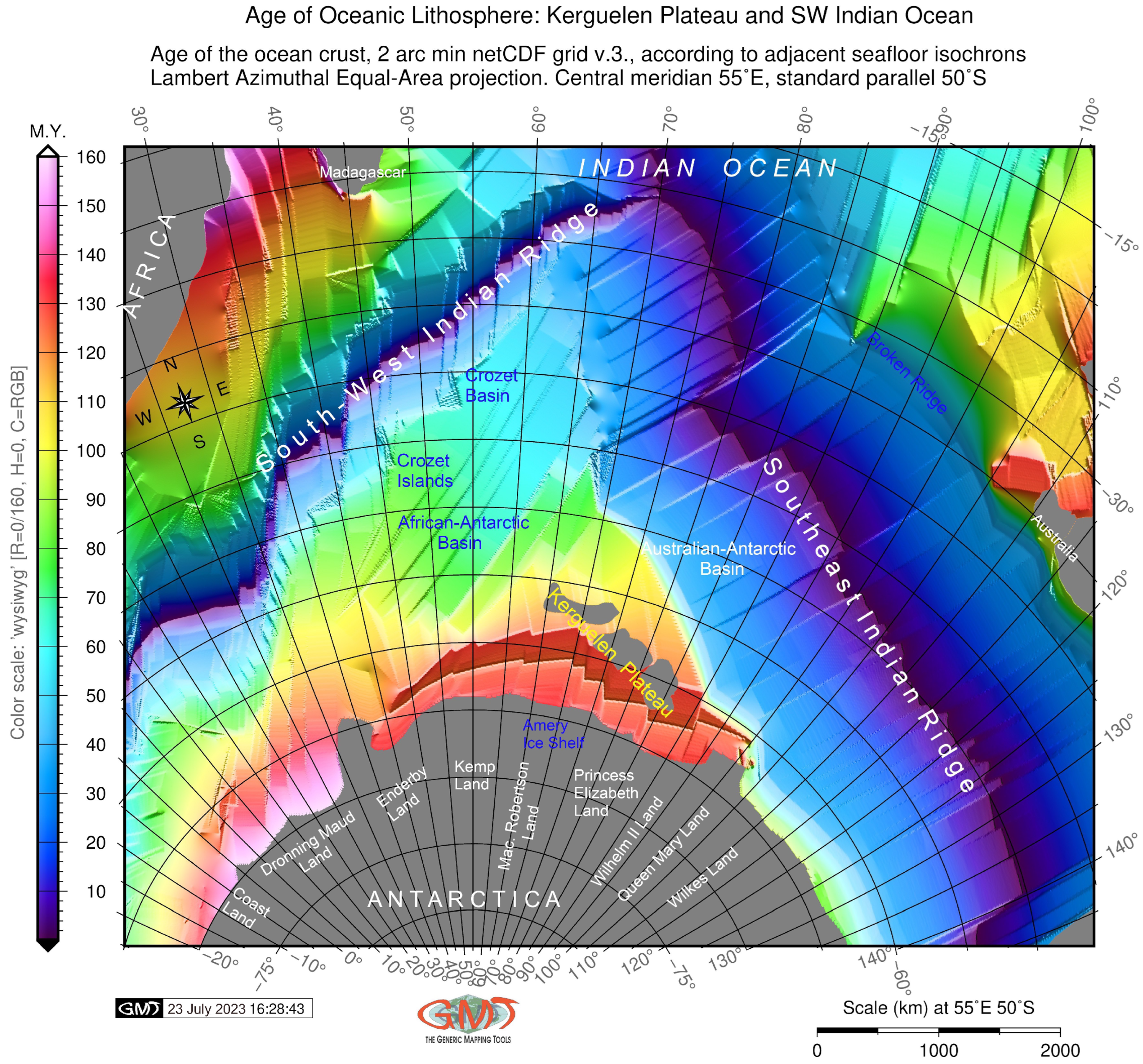
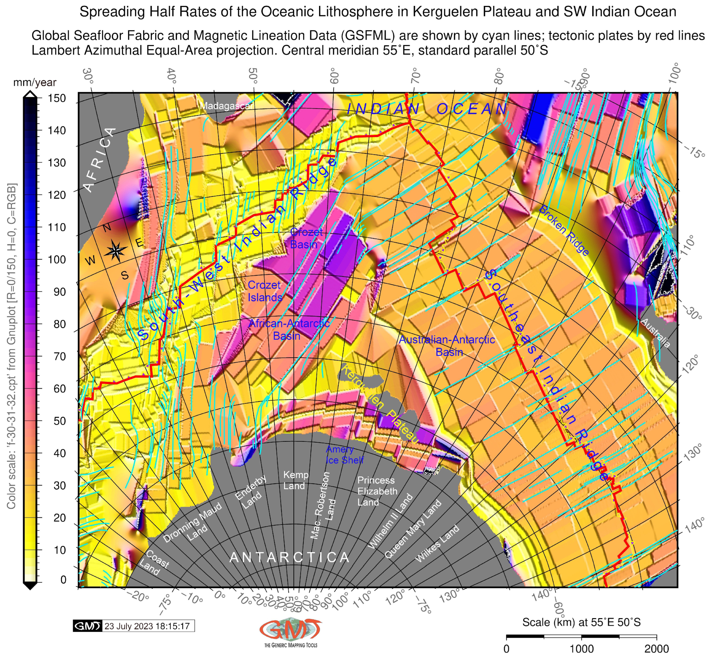
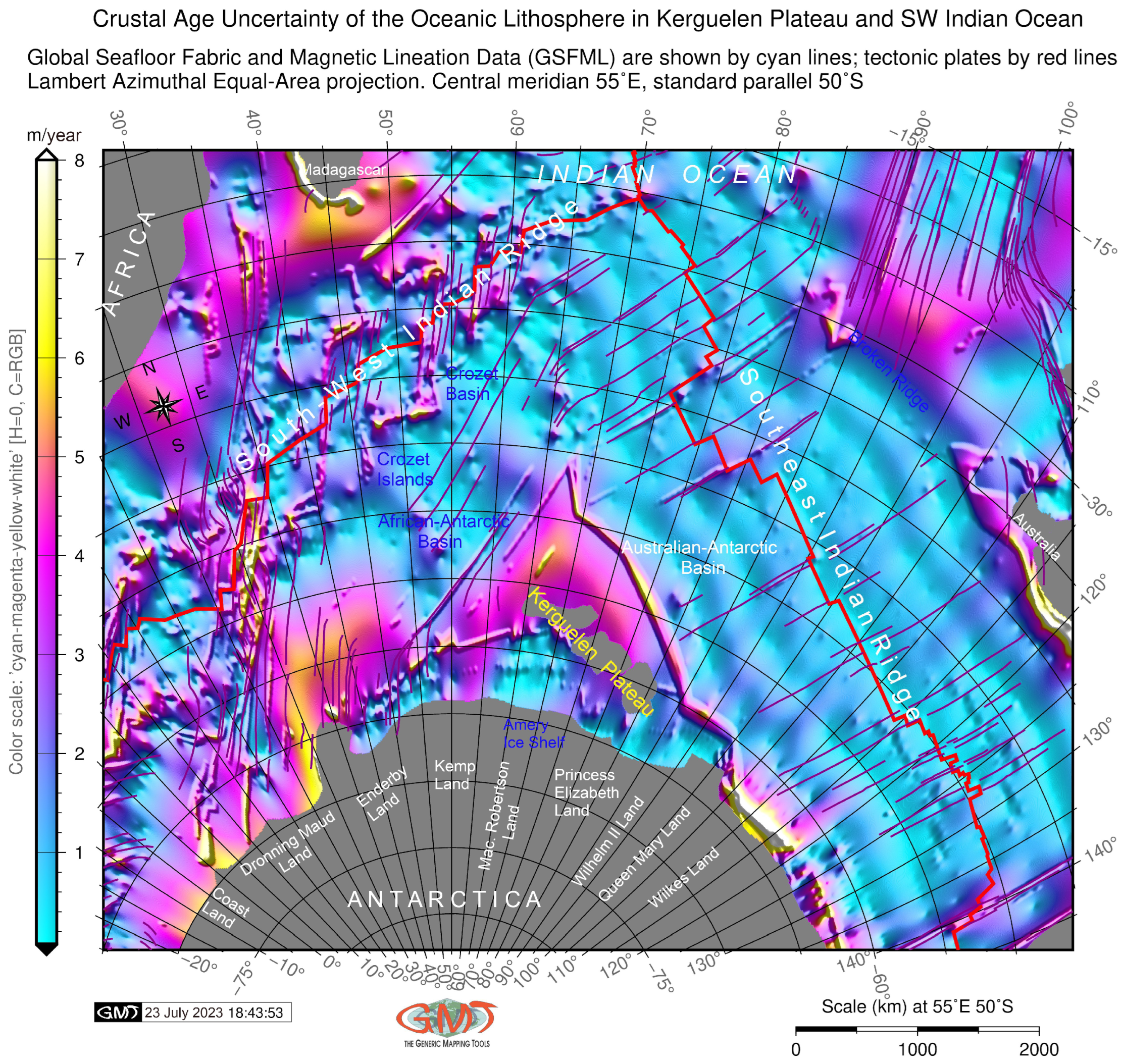
Mapping the age, age uncertainty, spreading rates, and spreading asymmetries of the Kerguelen Plateau is executed using raster grids with a 2-min resolution, as shown in Figure 4. These grids are reprojected to the Lambert Azimuthal Equal-Area projection utilizing data from major features within the Indian Ocean basin. The ‘psxy’ module is employed to add vector lines representing mid-ocean ridges, tectonic plates, and lithospheric plates. This provides a depiction of the borders of the Indian, African, and Australian plates, as seen in Figure 4. Spreading half rates of the ocean crust are visually presented using the 2-arc-minute netCDF grid v.3.6 from NOAA. Similarly, tectonic slab contours are added via the ‘psxy’ module of GMT. Multiple grids are combined and displayed as plotted raster grids to illustrate age-depth relationships in the seafloor around the Kerguelen Plateau and southwest Indian Ocean. The complete scripts are available in Appendix A of this study, with Listing A2 utilized for mapping the age of the oceanic lithosphere over the Kerguelen Plateau, Listing A3 for mapping asymmetries in crustal accretion on conjugate ridge flanks over the Kerguelen Plateau, Listing A4 for visualizing spreading half rates of the oceanic lithosphere in the Kerguelen Plateau and SW Indian Ocean, and Listing A5 for mapping crustal age uncertainty of the oceanic lithosphere over the Kerguelen Plateau, as depicted in Figure 5.
3.2.3. Mapping Sediment Thickness
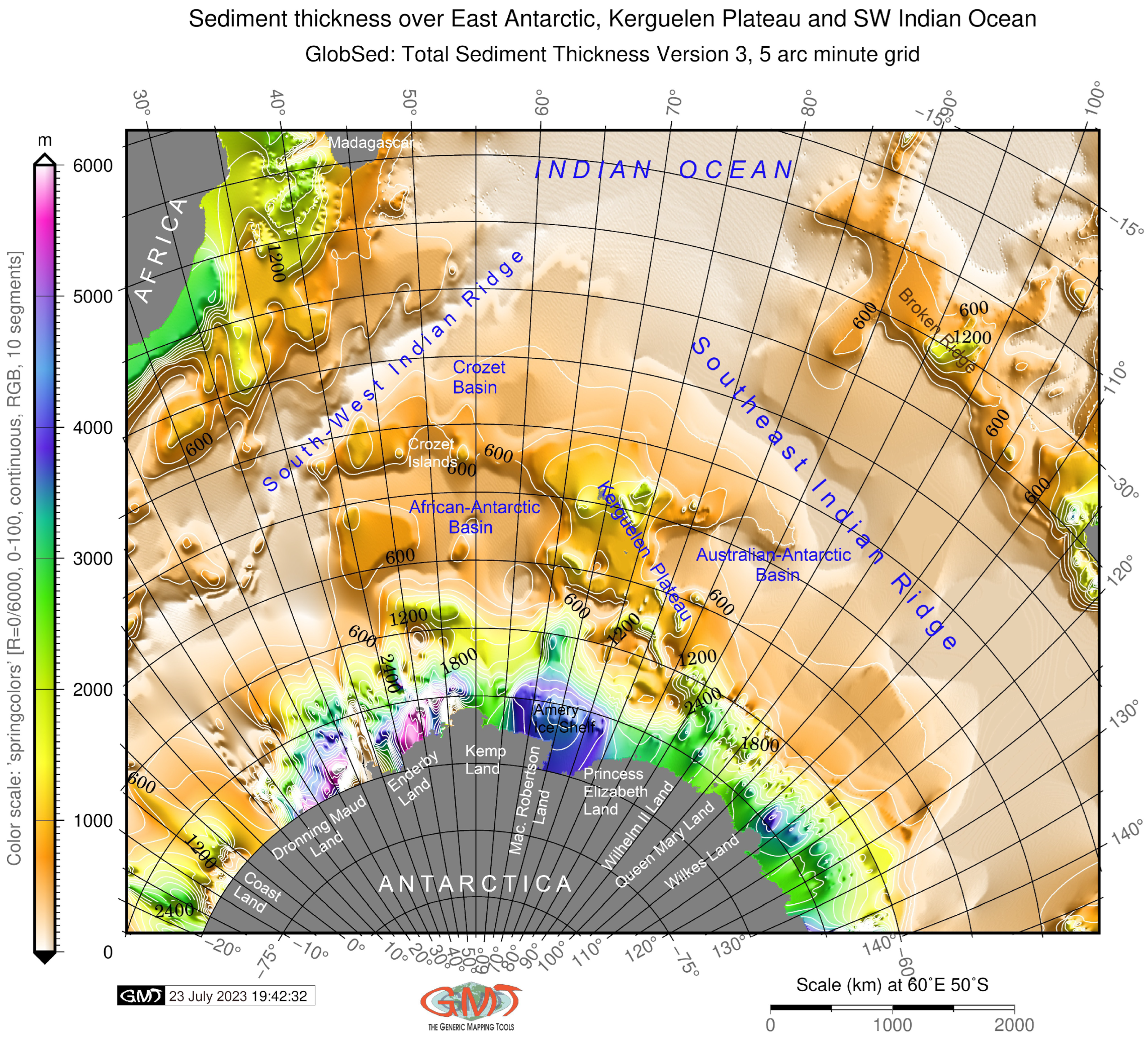
A representation of the GlobSed 5-arc-minute total sediment thickness grid is extracted from the global raster grid on a target location of the Kerguelen Archipelago area and surrounding regions using ‘grdcut’ command, which selects the file. The amplitude of values is checked using the Geospatial Data Abstraction Library (GDAL) library embedded in GMT using the ‘gdalinfo’. Based on the range of the values, the colour palette table is defined accordingly and presented using the ‘psscale’ module. This module is configured with parameters specifying the geographic location for each element on the map. The ‘-Dg’ command is employed to define the position of the colour scale on the map using coordinates. Furthermore, grid annotations and graticules are added utilizing the ‘psbasemap’ GMT module. The remaining part of the script, complete with added comments for concise explanations, is outlined in Listing A6 within the Appendix A of this study. This particular listing was utilized to create the map featured in Figure 6.
3.2.4. Geophysical Mapping
To emphasize features and subsurface characteristics that might not be apparent from geological data alone, maps of gravity anomalies were generated using gravity datasets projected onto the Lambert Equal-Area Azimuthal Projection for consistency with other maps. The complete scripts for creating these geophysical maps can be found in Appendix A, with Listing A7 detailing the process for free-air gravity anomalies and Listing A8 for vertical gravity gradient. The crucial lines of code are summarized below.
For free-air gravity anomalies, the ‘img2grd’ module was initially employed to convert the image from the .IMG format into GRD format. The projection was defined using the ‘-JU43/6.0i’ flag within the ‘grdimage’ module. The extent of the region was specified using the ‘-R’ command, and this information was subsequently passed to subsequent modules using the ‘-R -J’ flags.
In the case of the vertical gravity gradient map, a satellite-derived grid sourced from altimeters CryoSat-2 and Jason-1/2 [115] was used. This dataset facilitated the identification of ridge propagation on the seafloor.
Due to GMT’s ability to process each feature only once and utilize relevant modules (‘psbasemap’, ‘grdcontour’, ‘psscale’), it boasts a high processing speed. This technical advantage empowers GMT to efficiently handle grids encompassing extensive geographic areas in a matter of seconds. With an understanding of the seafloor’s geological and geophysical structure, GMT demonstrates rapidity and proficiency in mapping.
By adjusting projection parameters, the algorithm concentrates on key seafloor features within the desired scale and projection. Additionally, the GMT-based framework excels in determining the location, scope, and boundaries of mid-ocean ridges and significant basins. Through cartographic generalization involving the gap in isolines, redundant bathymetric features can be eliminated. This process identifies pertinent and nonrepetitive features, underscores correlations between geophysical settings, gravity, and magnetic anomalies, and facilitates their comparison with geodetic anomalies. Consequently, GMT offers an effective approach to map and visualize seafloor structures.
3.2.5. Mapping Magnetic Anomalies
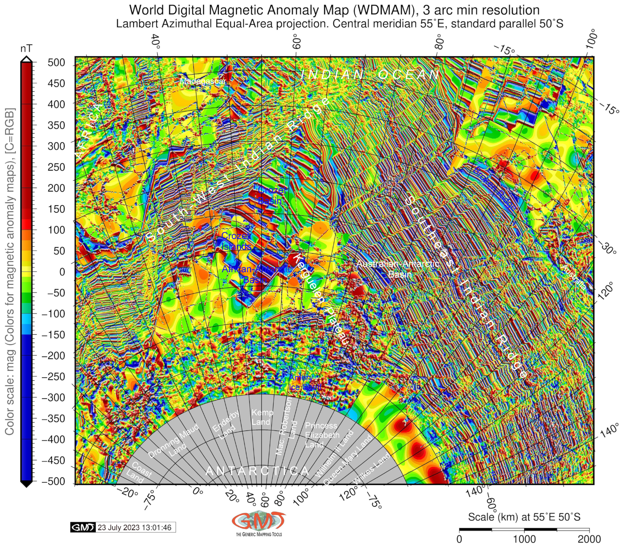
To map the magnetic anomalies, two different grids were used—the WDMAM and the EMAG2. The first was a subset from the global grid embedded in the GMT using the ‘grdcut’ module, and the second was obtained from the existing raster file of EMAG 2-min resolution grid. As a result, GMT offers flexibility in data processing through two approaches: utilizing pre-existing stored files and accessing embedded grids available within the system remotely. Subsequently, the images were rendered using the ‘grdimage’ module, accompanied by color palettes tailored to the data distribution range across the Kerguelen Plateau and the adjacent southwestern Indian Ocean. The ‘makecpt’ module was employed for this purpose. For a comprehensive view of the GMT scripts for both maps visualized with WDMAM and EMAG2, refer to Listings A9 and A10 in Appendix A.8.
3.2.6. Mapping Geoid Anomalies
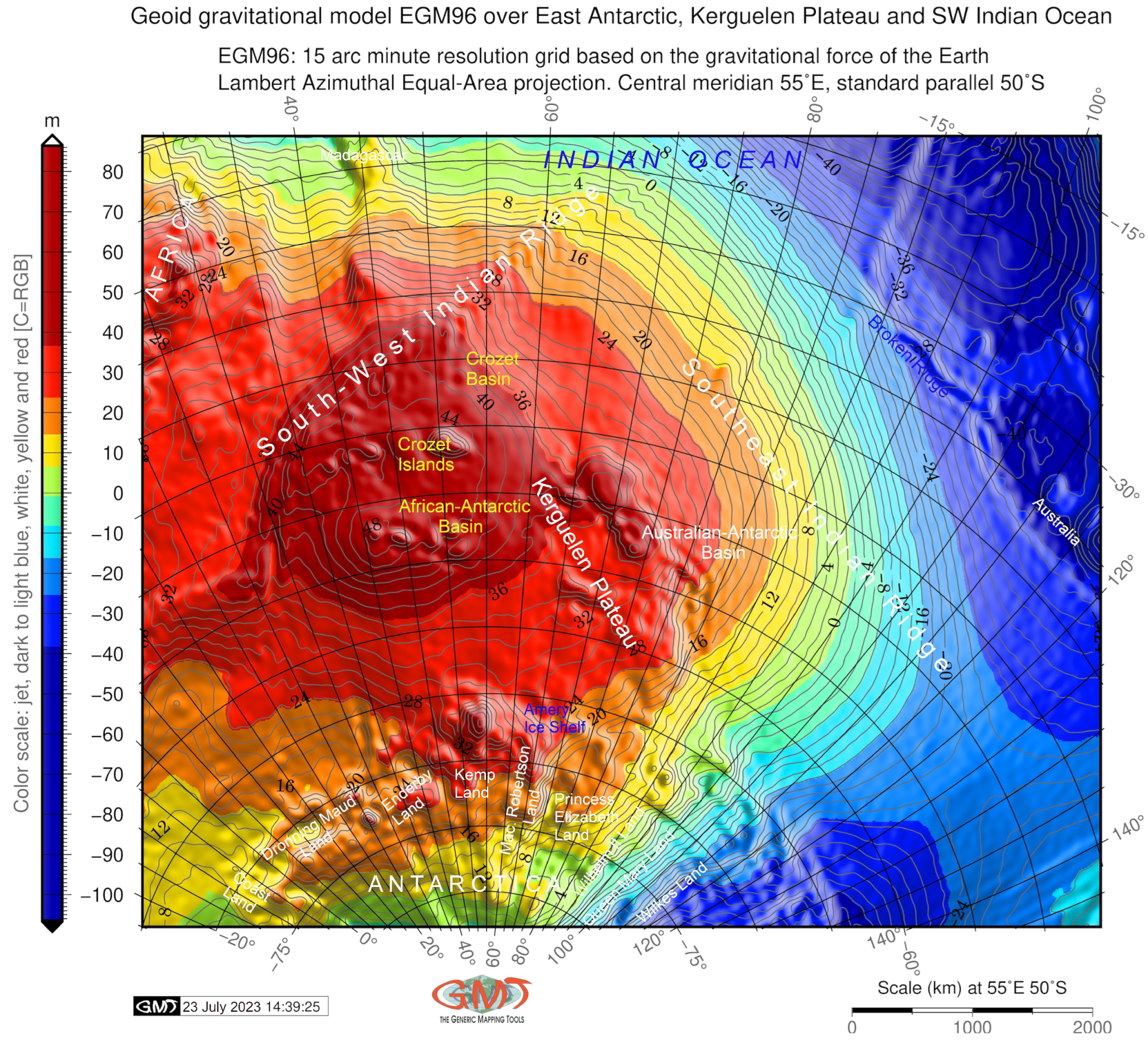
The map of geoid inundations was created using the EGM96 dataset through the GMT script, with each module defining specific elements on the map. To achieve effective mapping, the scripts were executed from the console, tailoring the geoid plotting to target concepts such as projections, grids, colour palettes, raster extents, and annotations. The stepwise definition of these cartographic elements is evident on the geoid maps, as demonstrated in the script provided in Listing A11. This approach to data visualization ensures high levels of automation in data processing through GMT, surpassing conventional tools.
Significant features such as geoid undulations, seafloor isochrons, basement depth isolines, and asymmetries in crustal accretion are influenced by the asthenospheric flow from Kerguelen’s mantle plumes to the spreading Southwest and Southeast Ridges. Mapping these data reveals insights into seafloor attributes and enables comparisons with the geological structure and geodynamics. Consequently, mapping multi-source topographic and geophysical datasets allows for the comparison of features using consistent projections. However, it is important to note that real-world seafloor features are seldom identical due to various factors impacting bathymetry, although they may exhibit strong correlations. To address this, GMT scripts can be adapted to different scales to map features in more detailed views. In order to assess the influence of geophysical and geological settings on seafloor structure using GMT’s capabilities, numerous cartographic re-projections were generated. Each map represented selected seafloor features at varying levels of detail. The Lambert azimuthal equal-area projection was ultimately chosen as the optimal projection for its applicability across all maps, ensuring comparability and coherence.
4. Results and Discussion
Automatic matching of topographic and geophysical grids with high accuracy is essential for complex geologic–tectonic investigations. This paper demonstrated the use of scripting algorithms of GMT. These algorithms were applied for plotting eleven thematic maps covering the south-west segment of Indian Ocean and East Antarctic using bathymetric, geodynamic and high-resolution geophysical datasets on gravity (Figure 7 and Figure 8). Cartographic scripts by GMT, as demonstrated in this research, provide visualized information on the geodynamic and geophysical setting of remotely located areas such as Kerguelen Plateau. During the cartographic process and workflow, the scripts enable us to save time through the increased speed of mapping due to the high level of automation.
The programming concept of GMT enables us to better tune and adjust the layout of the cartographic plots in various scales and focus on a specific area for comparability of maps in a series. Such compatibility facilitates the evaluation of correlations among various geophysical and bathymetric features that have developed over the extensive history of the Kerguelen Archipelago. Furthermore, by utilizing geospatial analysis as a complementary technique, it becomes possible to compare and analyze the relationships within the geodynamic setting, such as age, spreading half rates of the ocean crust, asymmetry in crustal accretion on conjugate ridge flanks, and other variables. In this manner, GMT scripts offer an advanced cartographic method for visualizing datasets and extracting information through efficient data processing and modelling of geophysical properties of the seafloor.
These maps reveal the details of the structure of the seafloor in the Kerguelen Plateau. The results confirm that the dynamics of seafloor development, as reflected in the maps of oceanic crust age, asymmetries, and spreading rates of the south-west and southeast Indian ridges, are closely related to the major geophysical setting as depicted on the topographic, magnetic, and gravity grids. Additionally, the volcanic activity of the Kerguelen hotspot has a significant impact on the distribution of magnetic anomalies, which aligns with previous studies [116,117,118]. Overall, the results demonstrate that GMT scripting is a powerful and stable cartographic method that efficiently performs geophysical and bathymetric seafloor mapping. In the sections below, we discuss the obtained results on relevant maps, providing comments on the essential features and characteristics of the seafloor around the Kerguelen Plateau, south-west Indian Ocean, and East Antarctic.
4.1. Ocean Floor Formation
The advanced methods of visualization by GMT constitute an important element of the map content through detailed plotting of the depicted objects, which enables us to indicate qualitative and quantitative geophysical specifications for reference and analysis. Thus, the general physical-geographic structure of the Kerguelen Plateau is visible in Figure 1, which shows a morphological orientation of the archipelago in the NW-SE direction and an extent surpassing 2000 km in length. As can be seen, the northern and southern parts of the plateau are asymmetric, where the less expressed southern part is older and lies in deeper water in the topographically downlifted areas. Age, spreading rates, and spreading symmetry of the ocean crust indicate the gradual evolution steps of the ocean floor formation in the southwest Indian Ocean and around the Kerguelen Plateau. The geodynamic setting of the oceanic crust (Figure 2, Figure 3, Figure 4 and Figure 5) shows a strong relationship between the Kerguelen Plateau and the two mid-ocean ridges, which can be revealed from the analysis of the relief.
Relief is the main element of the seafloor since it reflects its geological structure and geodynamic history. Accordingly, the relief of the seafloor surface around the Kerguelen Plateau forms a continuously changing field of bathymetric heights. There are also sharp changes in altitude around the archipelago and mid-oceanic ridges. To depict the relief, GMT enables the modeling of isolines using the ‘grdcontour’ module and adjusted color gradients using methods of qualitative coloring of background and gradients according to the actual heights. At the same time, there are specific benefits of GMT techniques for mapping the hypsometric maps. Thus, the quantitative values of the relief make it possible to obtain absolute heights and elevations from the raster grid; the characteristics of the curvature and steepness of inclination can be obtained using the GMT module ‘grdtrack’ through cross-sectioning [119,120,121]. Moreover, GMT enables the modeling of the plasticity of the relief, that is, to depict a nonlinearity of the landform irregularities that form a visual image of the submarine terrain. This enables an analysis of the morphological conformity of the relief, which highlights major seafloor features, specific landforms, and their structure.
The age of the ocean crust was determined by interpolating the adjacent seafloor isochrons oriented towards the direction of seafloor spreading, as shown in Figure 2. This correspondence highlights the unique geophysical setting of the Kerguelen Plateau, underlain by the oceanic crust, which is strongly associated with its tectonic origin associated with volcanic hotspot and geologic history. The formation of the Southwest and the Southeast Indian Ridges is related to the uplift of the Kerguelen Plateau as a remnant of the Mesozoic oceanic basin existing after the separation of Gondwana. The comparison of the bathymetric map with geodynamic maps shows that seafloor heterogeneity around the Kerguelen Archipelago correlates with the seafloor spreading rates, where rougher basement is formed in the areas with the low half-spreading rate threshold (30–35 mm/year and lower). This correlation can be revealed by comparing the maps in Figure 1 and Figure 4. Such heterogeneity in seafloor patterns varies significantly in various basins of the Indian Ocean, depending on the geodynamic setting and the geologic development of the oceanic crust.
The gridded map of age of the ocean crust around the Kerguelen Plateau (Figure 2) shows a correlation with the observed spreading half rates of the lithosphere (Figure 4). Originally formed as a single structure, Kerguelen was then split by the seafloor spreading in the south-west sector of the Indian Ocean which resulted in the formation of the two segments of the archipelago [122] which are visible on the maps. Furthermore, the difference in volcanic activity between the northern and central parts of the Kerguelen Plateau, underlying Heard Island, indicates that it is located on a hotspot, with various parts of the islands experiencing the effects of the mantle plume on different scales [123,124,125]. This unstable position has an impact on the geodynamic patterns over the Kerguelen Islands, leading to a higher uncertainty in the age of the oceanic crust (Figure 5) compared to the adjacent areas. Additionally, the structure of the oceanic crust beneath the Kerguelen Plateau is similar to that beneath aseismic ridges such as the Crozet Rise and the Madagascar Ridge, providing evidence that it originates from active volcanism associated with a hot spot [126].
4.2. Sediment Thickness
Mapping sediment thickness using the 5-arc-minute GlobSed grid relies on the approximated modelling, which highlights the sedimentation trends around the Kerguelen Archipelago, Figure 6.
The analytical map showing sediment thickness (Figure 6) displays patterns and key characteristics of sediment distribution over the seafloor. Using GMT-based techniques of mapping, it is easy to highlight the variations in sediment accumulation in various parts of the ocean using an adjusted colour table and the actual range in the data on sediment thickness. Hence, the level of cartographic details depends on the depth of the analysis with regard to the geologic formation of the seafloor and sediment accumulation. The objects on the map show the main regions of accumulated sediments, the structure and trends in distribution, and special features and properties compared to the closeness of coastal areas. Thus, the distribution of the sediment thickness correlates with the age of the underlying oceanic lithosphere and its latitude, which can be noted by the comparison of maps in Figure 2 and Figure 6. Such correspondence is especially visible for higher values of the sediment thickness near the shorelines of the Antarctic, Amery Ice Shelf (3000–4000 m), Enderby Land (over 4000 m) and the Kerguelen Plateau (2000–3000 m).
A higher level of sediment thickness in these areas may also indicate earlier processes of subaerial erosion that occurred before subsidence and associated sedimentation. The rifting process that took place during the Late Paleogene resulted in changes in the Tertiary sediment facies of Kerguelen, which were influenced by the evolution of the Antarctic environment [127]. Sediments covering the Kerguelen Plateau include pillow lavas, tuffaceous sediments, and marine siltstones that were deposited since the late Miocene [128]. These sediments continue as a thick sequence of Cenozoic sediments (over 5000 m) within the Enderby Basin to the southwest of the Kerguelen Plateau (Figure 6).
The correlations observed between sediment thickness (Figure 6) and the age of the oceanic lithosphere (Figure 2) demonstrate the role of ocean floor formation in influencing the pattern of distribution and accumulation of sediments.
Moreover, the analytical map of sediment thickness reflects smaller features and details compared to the bathymetry of the southwest Indian Ocean. Hence, comparing the map of sediment thickness with the bathymetry enables us to detect associations, for example, high values of sediment thickness in the region of Dronning maud Land in the Antarctic, which can be associated with the effects from the processes of weathering and coastal erosion, factors of higher curvature in slopes and topographic variations in heights in the coastal areas. Other important factors increasing the accumulation of the sediments around the Kerguelen and the adjacent area include glacial processes and the turbidity of the ocean currents. Hence, intense circulation results in the accumulation of the large sediment fields with values over 3000 m.
These effects can be attributed to the Antarctic circumpolar currents that started around the Eocene-Oligocene periods and have continued until the present time. These currents constitute the strongest current system in the oceans, directed clockwise around the South Pole, and they significantly influence the adjacent sub-Antarctic regions, such as Kerguelen [129,130].
The general orientation of areas with maximal sedimentation is consistent with the sediment-filled troughs stretching in a NW-SE direction. These troughs are associated with the overall NW-SE orientation of Kerguelen and the axes of tectonic faults. The high values in sediment thickness around the Kerguelen Plateau, particularly contoured by the ridge isolines along its eastern margin, are associated with depositions resulting from bottom currents directed westwards.
4.3. Free-Air Gravity Anomaly and Vertical Gravity Gradients
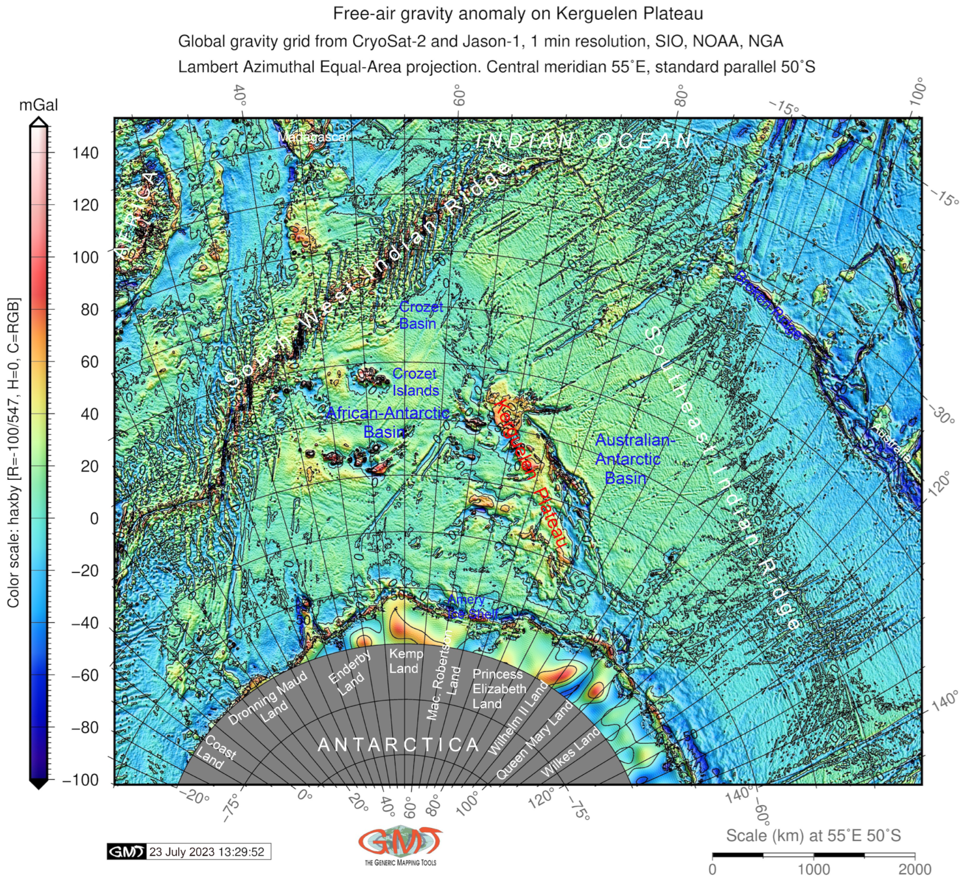
The visualized marine gravity field over the Kerguelen Plateau region and the adjacent areas of the south-west Indian Ocean are shown in Figure 7. The comparison of the gravity roughness with the map of the half-spreading rates (Figure 4) and sediment thickness (Figure 6) shows the relationship between the speed of the spreading of mid-ocean ridges and roughness of the seafloor basement. Such phenomena are explained by the effects from the process of mid-ocean ridge formation. Other factors include the associated magma flows, spreading directions in Mesozoic and isochron orientations of the age of the oceanic crust, which affect current bathymetric and gravity patterns [131]. Furthermore, the gravity highs around the Kerguelen Plateau and Heard Island correspond to the maximal bathymetric elevations. These gravity highs indicate the presence of seamounts formed by Miocene basalts erupted during volcanic activity in the southern Indian Ocean. This volcanic activity contributed to the formation of a large igneous province [132].
The GMT-based geophysical maps enable us to determine the location and spatio-temporal structure of gravity phenomena that indicate on geological processes, their mutual relationships, and connections with topography. Such analysis supports the identification of trends and dynamics in seafloor development. It helps obtain quantitative characteristics from geophysical data and estimate both the highest and lowest values in gravity grids. In turn, zoning and classification of gravity variations helps to forecast changes in gravity anomalies over the seafloor of the Indian Ocean. Hence, the analysis of maps shows that the values of the free-air gravity over the Kerguelen are higher than in the surrounding areas and reach up to 80 mGal (Figure 8). In contrast, lower values are associated with the bathymetric depressions and have values of −40 to −60 mGal. Furthermore, the abyssal plain is characterized by the medium values of 0–20 mGal, Figure 8. This well illustrates the existing correlation of the free-air gravity anomalies with the distribution of topographic highs and depressions on the seafloor since they are strongly influenced by a gravitational effect of the distributed topographic masses that are caused by the differences in elevation.
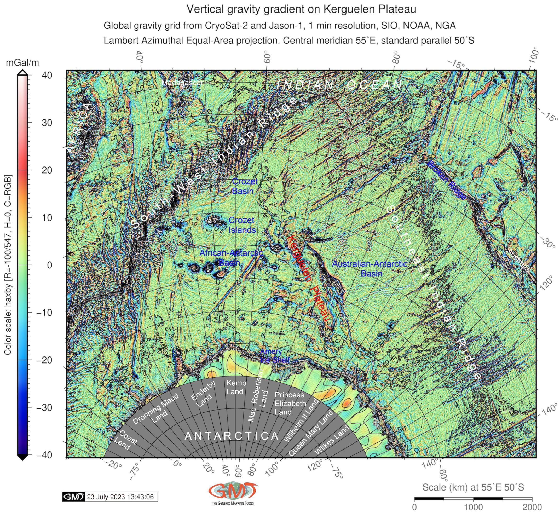
Figure 8 displays the mapping outputs for the vertical gradient over the Kerguelen and the southwest Indian Ocean, showcasing the effects of different locations. The visualized map demonstrates a crucial property of gravitational systems, such as free-air gravity, which is not only subject to the effects of geographic location and the latitude of the selected measurement regions but also the altitude of the Earth’s surface. This is because greater altitude implies a greater distance from the Earth’s center, which in turn affects gravity values. Moreover, the vertical gravity gradient identifies variations in gravity with changes in topographic elevations, as depicted in Figure 8. The comparison of gravity datasets provides additional information on the distribution of major geological and seafloor structures, considering the variations of geophysical fields.
Furthremore, the comparison of the vertical gradient and free-air gravity map (Figure 7 and Figure 8) with the topographic map (Figure 1) illustrates the effects of seafloor structure and the distribution of the oceanic bed on gravity, which shows that the highest values correspond to the Kerguelen Plateau and other rises, while lower values are generally associated with topographic depressions.
4.4. Magnetic Anomalies over Kerguelen Plateau
The anomaly of the magnetic intensity at an altitude of 5 km above mean sea level over the Kerguelen Plateau is shown in Figure 9.
Here, high heterogeneity in the geophysical data is related to the past volcanism over the Kerguelen Plateau, including the voluminous basaltic flooding originated from a deep hot spot as an asthenospheric source of mantle plume product. This resulted from the processes of slab dynamics and tectonic plate movements in the southwestern segment of the Indian Ocean. In this regard, combining the data from the WDMAM and EMAG2 (Figure 9 and Figure 10) data on terrestrial gravity fields (Figure 7 and Figure 8) for comparison with maps on oceanic crust development (Figure 2, Figure 3, Figure 4 and Figure 5) presents an integrated GMT-based geophysical analysis.
Crustal volume contributes to the decreased amplitude of the magnetic anomaly around the Kerguelen, as can be seen in Figure 10, with lower values of around −500 mGal. The analysis of the magnetic anomaly patterns in the SW Indian Ocean supports the hypothesis of the spreading seafloor with variations in the oceanic crustal block movements, as reported earlier [133]. This phenomenon is evident from the different magnetic patterns observed over the mid-ocean ridge. Moreover, the comparison of Figure 10 with Figure 5 reveals that seafloor age uncertainties for grid cells coincide with the marine magnetic anomaly identified around the Kerguelen Islands. This correlation is also observed for the conjugate ridge flanks (Figure 3 and Figure 10).
The Earth Magnetic Anomaly Grid (EMAG2) offers the opportunity to assess magnetic-gravity field relationships as descriptors, going beyond the traditional analysis of gravity and magnetic anomalies. Magnetic anomalies arise from geological and topographic features that alter local magnetic fields, making it crucial to comprehend their correlation with geophysical phenomena and topography. For instance, scrutinizing local magnetic anomaly patterns in the southwest Indian Ocean reveals associations with oceanic crust formation, seafloor spreading, and subduction zones. Moreover, the age of oceanic crust and spreading rates, resulting from land accretion and extensive volcanism of the Kerguelen Plateau, are linked to the historical geological development of the region, as mentioned previously [134].
The EMAG-2 and WDMAM grids employed for plotting magnetic anomalies exhibit varying levels of grid detail, allowing insight into the subsurface structure of the seafloor around the Kerguelen Plateau and the composition of the Earth’s crust in the southwest Indian Ocean. The magnetic fabric data correlate with hotspot activities and active volcanism, particularly prominent over the central and northern sectors of the archipelago [135,136,137]. Furthermore, intermediate crustal thickness values within the oceanic crust beneath the Kerguelen Plateau and large-amplitude magnetic anomalies across the archipelago point to the plateau’s oceanic origin, attributed to plate volcanism resulting from tectonic plate activity, as previously reported [138,139]. Therefore, the distinctive magnetic patterns evident in Figure 10 maps correspond to heightened hotspot activity and the associated lava flows.
Deeper masses, asthenospheric upwelling, and mantle plume-driven convection are geodynamic processes that influence the magnetic properties of the Earth’s surface. Moreover, through data analysis, a deeper understanding of the impact of geophysical settings on the distribution of positive and negative magnetic undulations emerges, with the former situated over the Kerguelen Islands and the latter in the eastern regions and southwest of Australia. This analysis enables the assessment of variations in geophysical grids through comparative map analysis. Thus, the cartographic depiction of geophysical and magnetic datasets offers advanced methods for extracting information about seafloor formation and interconnected geophysical processes.
4.5. Geoid Models
The geopotential model over the Kerguelen, based on the EGM96 dataset, is illustrated in Figure 11. The variations in the geoid across the Kerguelen Plateau highlight the ongoing isostatic compensation of the archipelago due to its low-density mantle. Consequently, the high anomalies in the geoid level above the Kerguelen Plateau can be attributed to the significant volcanic activity associated with the formation of ridges on the hot lithosphere. This volcanic activity is reflected in the exceptionally thick crust beneath the Kerguelen, resulting in geoid values exceeding 40 m (Figure 11), surpassing the normal thickness of the oceanic crust. These findings corroborate previous studies investigating the geoid in the Kerguelen Archipelago, which documented anomalous thickness in this region [140]. This isostatic compensation, linked to anomalously high geoid values, corresponds to the rugged elevated terrain in regions experiencing active tectonic uplift. These observations shed light on processes occurring in the upper mantle [141].
A comparison of the geoid map with topography (sf. Figure 1 and Figure 11) implies an existing correlation between the continued geodynamic processes in the south-west Indian Ocean and the topographic structure of the Kerguelen Archipelago. Moreover, this proves a high positive correlation between the geoid height and deep structure of the seafloor topography, as also noted earlier for the regions of large plateaus and swells [142].
5. Conclusions
As demonstrated in this study, the GMT-based mapping approach offers a wide range of cartographic functions for comprehensive spatio-temporal modelling and data visualization through an automated scripting approach. Utilizing GMT for cartographic tasks provides various modules and methods for representing different types of data, making it applicable in diverse fields of geomatics. The advantages of employing GMT in cartographic workflows are manifold. It enables highly automated plotting, facilitating rapid visualization of complex elements and features such as geographical, geological, oceanological, and geomorphological characteristics.
Furthermore, GMT supports multiple formats, encompassing both raster and vector data, and accommodating various classes and types of information. Leveraging the technical capabilities of GMT within cartographic workflows allows for common modelling and basic statistical analysis of spatial data, enhancing the understanding of their properties.
Analyzing a multitude of maps generated using GMT scripts reveals the consistency in depicted objects, facilitating their recognition and interpretation. The broad spectrum of GMT modules integrates scientific and technical methodologies for cartographic visualization and geospatial analysis. This unification aids in feature detection, recognition, and related research support.
Consequently, GMT-based mapping enables the amalgamation of maps for spatial analysis of intricate processes, objects, and phenomena, such as seafloor structures. This approach proves invaluable in addressing scientific and practical challenges within the realms of geophysics and geodynamics. The flexibility of GMT’s syntax, the quality of its cartographic outputs, and its compatibility with various operating systems and computing devices all contribute to its effectiveness.
Given the success and applicability showcased in the executed GMT scripts–characterized by syntax flexibility, high-quality cartographic outputs, and compatibility across different platforms–it is foreseeable that this GMT-based cartographic method can be extended to study seafloor structures in other oceanic regions, considering varying geologic conditions and geodynamic evolutions.
Global surveillance of the seafloor through the use of altimeter satellites and gravity measurements has unveiled significant geophysical anomalies. Integrating data on magnetic field intensity, bathymetry, and deep seafloor geodynamics allows for an evaluation of the interrelations among these processes. This ongoing global surveillance continues to generate extensive high-resolution datasets. However, effectively analyzing these datasets in ever-higher spatial resolutions demands advanced tools for automated analysis. The toolset of GMT scripts has demonstrated its effectiveness in the realm of seafloor bathymetric and geophysical mapping. This approach facilitates the visualization and mapping of diverse seabed features across varying scales and resolutions, aiming to detect correlations between magnetic anomalies, geophysical patterns, and their connections to present bathymetry. Such visualization offers comprehensive coverage of seafloor features across the near-global scale.
Direct seafloor surveys for observations are resource-intensive, involving the use of complex and costly equipment, such as multi-beam echo-sounding systems, for data collection, generation, and storage. Yet, the need persists for efficient datasets that can be readily visualized and analyzed. Utilizing high-resolution geophysical datasets provided by NOAA and USGS, processed through the advanced scripting capabilities of GMT, establishes a cartographic processing pipeline for swift, automated, and accurate seafloor mapping. Notably, GMT’s flexibility plays a pivotal role. A variety of GMT modules can be harnessed to process diverse geospatial data types, catering to different cartographic tasks. This flexibility allows for the adaptation and expansion of the proposed cartographic workflow, addressing larger-scale or smaller-scale mapping needs. The equilibrium between topographic gradients and geophysical grids vividly illustrates the links between seafloor patterns, the structure of the oceanic crust, and the processes within the lithospheric mantle.
From a cartographic perspective, this study underscores that the effective analysis of geologic-geophysical datasets within Earth sciences extends beyond utilizing isolated parameters (e.g., topographic maps) to encompass the selection of multiple datasets. The deep mantle processes, as reflected in geophysical data, intricately shape the seafloor formation. The methodology showcased in this study demonstrates how data from diverse sources (geophysical, topographic, geodetic, geodynamic) can be harnessed for comprehensive cartographic analysis using standardized workflows supported by scripts. This approach unveils additional insights into seafloor variability and the factors influencing ocean crust formation, strongly correlated with topographic patterns.
The cartographic approach exhibited here enables data assimilation and extension, not only across the Indian Ocean but also to other regions of the global ocean. For example, the Pacific Ocean boasts a rich tapestry of seafloor features, including vast abyssal plains, mid-ocean ridges, oceanic trenches, numerous seamounts, and continental shelves. These features present a fertile ground for investigating potential correlations between geophysical and magnetic anomalies and the heterogeneous seafloor patterns. In this context, the application of GMT for seafloor mapping in diverse oceanic regions serves as an ideal scenario for validating the cartographic scripting approach outlined in the methodological framework.
The series of maps presented, along with the comparison of the geophysical settings over the Kerguelen Plateau, underscores the superiority of script techniques over the GIS approach in terms of cartographic workflow automation. The compactness of GMT’s syntax allows for code reusability with modifications. However, there are limitations to consider. GMT necessitates parameter tuning in advance when handling map elements and adjusting projection parameters, as it lacks the ability to preview maps before script execution, being a console-based program. Furthermore, GMT cannot remove redundant features once plotted, requiring the script to be run again for corrections. In contrast, the GIS approach permits real-time adjustments to map layouts, enabling the correction of colour palettes and bathymetric details on the fly. GMT’s console-based nature mandates direct modifications to the script’s code to address cartographic challenges.
Funding
This research received no external funding.
Institutional Review Board Statement
Not applicable.
Informed Consent Statement
Not applicable.
Data Availability Statement
Not applicable.
Acknowledgments
The author sincerely thanks the two anonymous reviewers for critically reviewing this paper and for their constructive comments and useful suggestions, which have improved upon the initial version of this manuscript. The author is grateful to the Editorial Office of the Geomatics MDPI for support of this publication.
Conflicts of Interest
The authors declare no conflict of interest.
Abbreviations
The following abbreviations are used in this manuscript:
| DEM | Digital Elevation Model |
| EMAG-2 | Earth Magnetic Anomaly Grid 2 |
| EML | ERDAS Macro Language |
| ESRI | Environmental Systems Research Institute |
| GDAL | Geospatial Data Abstraction Library |
| GRACE | Gravity Recovery and Climate Experiment |
| GMT | Generic Mapping Tools |
| GRASS GIS | Geographic Resources Analysis Support System |
| GUI | Graphical User Interface |
| NOAA | National Oceanic and Atmospheric Administration |
| SRTM | Shuttle Radar Topography Mission |
| USGS | United States Geological Survey |
| UTM | Universal Transverse Mercator |
| WGM | World Gravity Model |
| WDMAM | World Digital Magnetic Anomaly Map |
Appendix A. GMT Scripts
Appendix A.1. GMT Script for Mapping Topography of the Kerguelen Region in Lambert Azimuthal Equal-Area Projection
| Listing A1. Mapping topography of the Kerguelen region in Lambert Azimuthal Equal-Area projection. |
 |
Appendix A.2. GMT Script for Mapping Age, Spreading Rates, Spreading Asymmetry and Age Uncertainty of the Ocean Crust
| Listing A2. Mapping age of the oceanic lithosphere over Kerguelen Plateau and SW Indian Ocean. |
 |
Appendix A.3. GMT Script for Mapping Asymmetries in Crustal Accretion on Conjugate Ridge Flanks: Kerguelen Plateau and SW Indian Ocean
| Listing A3. Mapping asymmetries in crustal accretion on conjugate ridge flanks: Kerguelen Plateau and SW Indian Ocean. |
 |
Appendix A.4. GMT Script for Mapping Spreading Half Rates of the Oceanic Lithosphere in Kerguelen Plateau and SW Indian Ocean
| Listing A4. Mapping spreading half rates of the oceanic lithosphere in Kerguelen Plateau and SW Indian Ocean. |
 |
Appendix A.5. GMT Script for Mapping Crustal Age Uncertainty of the Oceanic Lithosphere in Kerguelen Plateau and SW Indian Ocean
| Listing A5. Mapping crustal age uncertainty of the oceanic lithosphere in Kerguelen Plateau and SW Indian Ocean. |
 |
Appendix A.6. GMT Script for Sediment Thickness over the Kerguelen Plateau and SW Indian Ocean
| Listing A6. Mapping sediment thickness over the Kerguelen Plateau and SW Indian Ocean. |
 |
Appendix A.7. GMT Scripts for Geophysical Mapping over the Kerguelen Plateau
| Listing A7. Mapping free-air gravity anomalies over Kerguelen Plateau and SW Indian Ocean. |
 |
| Listing A8. Mapping vertical gravity gradient over Kerguelen Plateau and SW Indian Ocean. |
 |
Appendix A.8. GMT Scripts for Mapping Magnetic Anomalies over the Kerguelen Plateau
| Listing A9. Mapping magnetic anomalies by WDMAM over Kerguelen Plateau. |
 |
| Listing A10. Mapping magnetic anomalies by EMAG2 over Kerguelen Plateau. |
 |
Appendix A.9. GMT Scripts for Mapping Geoid Anomalies over the Kerguelen Plateau
| Listing A11. Mapping geoid anomalies in Kerguelen Plateau by EGM96. |
 |
References
- Papp-Váry, Á. The Science of Cartography. In Cartography Past, Present and Future; Rhind, D., Taylor, D., Eds.; International Cartographic Association, Pergamon: Amsterdam, The Netherlands, 1989; pp. 103–109. [Google Scholar] [CrossRef]
- Robinson, A.H. Cartography as an art. In Cartography Past, Present and Future; Rhind, D., Taylor, D., Eds.; International Cartographic Association, Pergamon: Amsterdam, The Netherlands, 1989; pp. 91–102. [Google Scholar] [CrossRef]
- Goodchild, M.F. Geographic Information Systems and Cartography. In International Encyclopedia of Human Geography, 2nd ed.; Kobayashi, A., Ed.; Elsevier: Oxford, UK, 2009; pp. 1–6. [Google Scholar] [CrossRef]
- Goodchild, M. GIS and Cartography. In International Encyclopedia of Human Geography; Kitchin, R., Thrift, N., Eds.; Elsevier: Oxford, UK, 2009; pp. 500–505. [Google Scholar] [CrossRef]
- Slocum, T.A.; Egbert, S.L. Cartographic Data Display. In Geographic Information Systems; Taylor, F., Ed.; Modern Cartography Series; Academic Press: Cambridge, MA, USA, 1991; Chapter 9; Volume 1, pp. 167–199. [Google Scholar] [CrossRef]
- Taylor, D.F. Perspectives on Visualization and Modern Cartography. In Visualization in Modern Cartography; Maceachren, A.M., Taylor, D.F., Eds.; Modern Cartography Series; Academic Press: Cambridge, MA, USA, 1994; Chapter 17; Volume 2, pp. 333–341. [Google Scholar] [CrossRef]
- Toms, S.; Parker, B.; Tucker, D.C.; Rubalcava, R. Python for ArcGIS Pro: Automate Cartography and Data Analysis Using ArcPy, ArcGIS API for Python, Notebooks, and Pandas; Packt Publishing: Birmingham, UK, 2022. [Google Scholar]
- Dobesova, Z.; Dobes, P. Comparison of visual languages in Geographic Information Systems. In Proceedings of the 2012 IEEE Symposium on Visual Languages and Human-Centric Computing (VL/HCC), Innsbruck, Austria, 30 September–4 October 2012; pp. 245–246. [Google Scholar] [CrossRef]
- Omran, A.; Dietrich, S.; Abouelmagd, A.; Michael, M. New ArcGIS tools developed for stream network extraction and basin delineations using Python and java script. Comput. Geosci. 2016, 94, 140–149. [Google Scholar] [CrossRef]
- Naghibi, S.A.; Hashemi, H.; Pradhan, B. APG: A novel python-based ArcGIS toolbox to generate absence-datasets for geospatial studies. Geosci. Front. 2021, 12, 101232. [Google Scholar] [CrossRef]
- Roberts, J.; Mwangi, R.; Mukabi, F.; Njui, J.; Nzioka, K.; Ndambiri, J.; Bispo, P.; Espirito-Santo, F.; Gou, Y.; Johnson, S.; et al. Pyeo: A Python package for near-real-time forest cover change detection from Earth observation using machine learning. Comput. Geosci. 2022, 167, 105192. [Google Scholar] [CrossRef]
- Lemenkova, P.; Debeir, O. Satellite Image Processing by Python and R Using Landsat 9 OLI/TIRS and SRTM DEM Data on Côte d’Ivoire, West Africa. J. Imaging 2022, 8, 317. [Google Scholar] [CrossRef] [PubMed]
- Vos, K.; Splinter, K.D.; Harley, M.D.; Simmons, J.A.; Turner, I.L. CoastSat: A Google Earth Engine-enabled Python toolkit to extract shorelines from publicly available satellite imagery. Environ. Model. Softw. 2019, 122, 104528. [Google Scholar] [CrossRef]
- Lemenkova, P.; Debeir, O. R Libraries for Remote Sensing Data Classification by K-Means Clustering and NDVI Computation in Congo River Basin, DRC. Appl. Sci. 2022, 12, 12554. [Google Scholar] [CrossRef]
- Dobesova, Z. Programming language Python for data processing. In Proceedings of the 2011 International Conference on Electrical and Control Engineering, Yichang, China, 16–18 September 2011; pp. 4866–4869. [Google Scholar] [CrossRef]
- Lemenkova, P. Cartographic scripts for seismic and geophysical mapping of Ecuador. Geografie 2022, 127, 195–218. [Google Scholar] [CrossRef]
- Aber, S.E.W.; Aber, J.W. Basic Map Concepts—The Science of Cartography. In Map Librarianship; Aber, S.E.W., Aber, J.W., Eds.; Chandos Information Professional Series; Chandos Publishing: Oxford, UK, 2017; Chapter 3; pp. 53–70. [Google Scholar] [CrossRef]
- Bascou, J.; Delpech, G.; Vauchez, A.; Moine, B.N.; Cottin, J.Y.; Barruol, G. An integrated study of microstructural, geochemical, and seismic properties of the lithospheric mantle above the Kerguelen plume (Indian Ocean). Geochem. Geophys. Geosyst. 2008, 9, 1–26. [Google Scholar] [CrossRef] [Green Version]
- Eshagh, M. Satellite gravimetry and isostasy. In Satellite Gravimetry and the Solid Earth; Eshagh, M., Ed.; Elsevier: Amsterdam, The Netherlands, 2021; Chapter 7; pp. 313–373. [Google Scholar] [CrossRef]
- Kapawar, M.; Mamilla, V.; Sangode, S. Anisotropy of magnetic susceptibility study to locate the feeder zone and lava flow directions of the Rajmahal Traps (India): Implications to Kerguelen mantle plume interaction with Indian Plate. Phys. Earth Planet. Inter. 2021, 313, 106692. [Google Scholar] [CrossRef]
- Peng, W.; Yang, T.; Shi, Y.; Bian, W.; Ma, Y.; Wang, S.; Jiao, X.; Ma, J.; Kang, Y.; Zhang, S.; et al. Role of the Kerguelen mantle plume in breakup of eastern Gondwana: Evidence from early cretaceous volcanic rocks in the eastern Tethyan Himalaya. Palaeogeogr. Palaeoclimatol. Palaeoecol. 2022, 588, 110823. [Google Scholar] [CrossRef]
- Zhang, Z.; Li, G.; He, X.; Zhang, L.; Dong, S.; Qing, C.; Liang, W.; Han, S. The evolution of Kerguelen mantle plume and breakup of eastern Gondwana: New insights from multistage Cretaceous magmatism in the Tethyan Himalaya. Gondwana Res. 2023, 119, 68–85. [Google Scholar] [CrossRef]
- Lemenkova, P. Variations in the bathymetry and bottom morphology of the Izu-Bonin Trench modelled by GMT. Bull. Geography. Phys. Geogr. Ser. 2020, 18, 41–60. [Google Scholar] [CrossRef]
- Tesauro, M.; Kaban, M.K.; Cloetingh, S.A. Global model for the lithospheric strength and effective elastic thickness. Tectonophysics 2013, 602, 78–86. [Google Scholar] [CrossRef]
- Battista, T.; O’Brien, K. Spatially Prioritizing Seafloor Mapping for Coastal and Marine Planning. Coast. Manag. 2015, 43, 35–51. [Google Scholar] [CrossRef]
- Lemenkova, P. The visualization of geophysical and geomorphologic data from the area of Weddell Sea by the Generic Mapping Tools. Stud. Quat. 2021, 38, 19–32. [Google Scholar] [CrossRef]
- Lemenkova, P. GEBCO Gridded Bathymetric Datasets for Mapping Japan Trench Geomorphology by Means of GMT Scripting Toolset. Geod. Cartogr. 2020, 46, 98–112. [Google Scholar] [CrossRef]
- Schlich, R.; Wise, S.W. The Geologic and Tectonic Evolution of the Kerguelen Plateau: An Introduction to the Scientific Results of Leg 120. Proc. Ocean. Drill. Program Sci. Results 1992, 120, 4. [Google Scholar]
- Veevers, J.J.; Li, Z.X. Review of seafloor spreading around Australia. II. Marine magnetic anomaly modelling. Aust. J. Earth Sci. 1991, 38, 391–408. [Google Scholar] [CrossRef]
- Negi, S.S.; Kumar, A.; Ningthoujam, L.S.; Pandey, D.K. Mapping the mantle transition zone beneath the Indian Ocean geoid low from Ps receiver functions. Tectonophysics 2022, 831, 229330. [Google Scholar] [CrossRef]
- Bénard, F.; Callot, J.P.; Vially, R.; Schmitz, J.; Roest, W.; Patriat, M.; Loubrieu, B. The Kerguelen plateau: Records from a long-living/composite microcontinent. Mar. Pet. Geol. 2010, 27, 633–649. [Google Scholar] [CrossRef]
- Ramana, M.V.; Ramprasad, T.; Desa, M. Seafloor spreading magnetic anomalies in the Enderby Basin, East Antarctica. Earth Planet. Sci. Lett. 2001, 191, 241–255. [Google Scholar] [CrossRef]
- Davis, J.K.; Lawver, L.A.; Norton, I.O.; Gahagan, L.M. New Somali Basin magnetic anomalies and a plate model for the early Indian Ocean. Gondwana Res. 2016, 34, 16–28. [Google Scholar] [CrossRef]
- Frey, F.; Coffin, M.; Wallace, P.; Weis, D.; Zhao, X.; Wise, S.; Wähnert, V.; Teagle, D.; Saccocia, P.; Reusch, D.; et al. Origin and evolution of a submarine large igneous province: The Kerguelen Plateau and Broken Ridge, southern Indian Ocean. Earth Planet. Sci. Lett. 2000, 176, 73–89. [Google Scholar] [CrossRef] [Green Version]
- Sreejith, K.M.; Krishna, K.S. Magma production rate along the Ninetyeast Ridge and its relationship to Indian plate motion and Kerguelen hot spot activity. Geophys. Res. Lett. 2015, 42, 1105–1112. [Google Scholar] [CrossRef]
- Lemenkova, P. Topography of the Aleutian Trench south-east off Bowers Ridge, Bering Sea, in the context of the geological development of North Pacific Ocean. Baltica 2021, 34, 27–46. [Google Scholar] [CrossRef]
- Falvey, D.A. Kerguelen Plateau Research Cruise. Eos Trans. Am. Geophys. Union 1985, 66, 641. [Google Scholar] [CrossRef]
- Watson, S.; Whittaker, J.; Halpin, J.; Williams, S.; Milan, L.; Daczko, N.; Wyman, D. Tectonic drivers and the influence of the Kerguelen plume on seafloor spreading during formation of the early Indian Ocean. Gondwana Res. 2016, 35, 97–114. [Google Scholar] [CrossRef]
- Lee, Y. Cartographic Data Capture and Storage. In Geographic Information Systems; Taylor, F., Ed.; Modern Cartography Series; Academic Press: Cambridge, MA, USA, 1991; Chapter 2; Volume 1, pp. 21–38. [Google Scholar] [CrossRef]
- Mori, M.; Corney, S.P.; Melbourne-Thomas, J.; Welsford, D.C.; Klocker, A.; Ziegler, P.E. Using satellite altimetry to inform hypotheses of transport of early life stage of Patagonian toothfish on the Kerguelen Plateau. Ecol. Model. 2016, 340, 45–56. [Google Scholar] [CrossRef] [Green Version]
- Cotté, C.; Ariza, A.; Berne, A.; Habasque, J.; Lebourges-Dhaussy, A.; Roudaut, G.; Espinasse, B.; Hunt, B.; Pakhomov, E.; Henschke, N.; et al. Macrozooplankton and micronekton diversity and associated carbon vertical patterns and fluxes under distinct productive conditions around the Kerguelen Islands. J. Mar. Syst. 2022, 226, 103650. [Google Scholar] [CrossRef]
- Maraldi, C.; Lyard, F.; Testut, L.; Coleman, R. Energetics of internal tides around the Kerguelen Plateau from modeling and altimetry. J. Geophys. Res. Ocean. 2011, 116, 1–10. [Google Scholar] [CrossRef] [Green Version]
- Verfaillie, D.; Favier, V.; Dumont, M.; Jomelli, V.; Gilbert, A.; Brunstein, D.; Gallée, H.; Rinterknecht, V.; Menegoz, M.; Frenot, Y. Recent glacier decline in the Kerguelen Islands (49°S, 69°E) derived from modeling, field observations, and satellite data. J. Geophys. Res. Earth Surf. 2015, 120, 637–654. [Google Scholar] [CrossRef] [Green Version]
- Yamamoto, K.; Fukuda, Y.; Doi, K.; Motoyama, H. Interpretation of the GRACE-derived mass trend in Enderby Land, Antarctica. Polar Sci. 2008, 2, 267–276. [Google Scholar] [CrossRef] [Green Version]
- Mathieu, L.; Byrne, P.; Guillaume, D.; van Wyk de Vries, B.; Moine, B. The field and remote sensing analysis of the Kerguelen Archipelago structure, Indian Ocean. J. Volcanol. Geotherm. Res. 2011, 199, 206–215. [Google Scholar] [CrossRef]
- Cowley, S.; Mann, P.; Coffin, M.; Shipley, T.H. Oligocene to Recent tectonic history of the Central Solomon intra-arc basin as determined from marine seismic reflection data and compilation of onland geology. Tectonophysics 2004, 389, 267–307. [Google Scholar] [CrossRef]
- Lemenkova, P. Dataset compilation by GRASS GIS for thematic mapping of Antarctica: Topographic surface, ice thickness, subglacial bed elevation and sediment thickness. Czech Polar Rep. 2021, 11, 67–85. [Google Scholar] [CrossRef]
- Kovalevsky, E.V.; Kharchenko, V.I. Integrated interpretation of marine engineering geological and geophysical data on the principles of expert system technology: Kovalevsky, E V; Kharchenko, V I Geophys ProspectV40, N8, Nov 1992, P909–923. Int. J. Rock Mech. Min. Sci. Geomech. Abstr. 1993, 30, A234. [Google Scholar] [CrossRef]
- Abuamarah, B.A.; Nabawy, B.S.; Shehata, A.M.; Kassem, O.M.; Ghrefat, H. Integrated geological and petrophysical characterization of oligocene deep marine unconventional poor to tight sandstone gas reservoir. Mar. Pet. Geol. 2019, 109, 868–885. [Google Scholar] [CrossRef]
- Veevers, J.J.; Powell, C.M.; Roots, S.R. Review of seafloor spreading around Australia. I. synthesis of the patterns of spreading. Aust. J. Earth Sci. 1991, 38, 373–389. [Google Scholar] [CrossRef]
- Lemenkova, P. Geodynamic setting of Scotia Sea and its effects on geomorphology of South Sandwich Trench, Southern Ocean. Pol. Polar Res. 2021, 42, 1–23. [Google Scholar] [CrossRef]
- Hill, P.J. Seafloor Magnetic Patterns: Seafloor Spreading and Magnetization in the Southern Ocean. Explor. Geophys. 1986, 17, 40–42. [Google Scholar] [CrossRef] [Green Version]
- Nougier, J. Bibliographie Cartographique des Iles Kerguelen/par Jacques Nougier; Institut Geographique National: Paris, France, 1968; p. 55. Available online: https://catalogue.nla.gov.au/Record/2259953 (accessed on 10 July 2023).
- Petit, G.; Petit, G. Edgar Aubert de la Rüe. — Etude géologique et géographique de l’Archipel de Kerguelen. Rev. D’Écologie 1933, 3, 63–64. [Google Scholar]
- Recq, M. Contribution a l’etude de la structure profonde du banc de Crozet (Ocean Indien Austral). Mar. Geol. 1989, 88, 133–144. [Google Scholar] [CrossRef]
- Operto, S. Structure et Origine du Plateau de Kerguelen (Océan Indien Austral): Implications Géodynamique. Modélisation de Données Sismiques Grand-Angle Marines. Ph.D. Thesis, Université Pierre et Marie Curie, Paris, France, 1995. [Google Scholar]
- Ramsay, D.C.; Colwell, J.B.; Coffin, M.F.; Davies, H.L.; Hill, P.J.; Pigram, C.J.; Stagg, H.M.J. New findings from the Kerguelen Plateau. Geology 1986, 14, 589–593. [Google Scholar] [CrossRef]
- Breton, T.; Nauret, F.; Pichat, S.; Moine, B.; Moreira, M.; Rose-Koga, E.F.; Auclair, D.; Bosq, C.; Wavrant, L.M. Geochemical heterogeneities within the Crozet hotspot. Earth Planet. Sci. Lett. 2013, 376, 126–136. [Google Scholar] [CrossRef]
- Guglielmi, M. Etude Géophysique du Plateau de Kerguelen. Ph.D. Thesis, Université Louis Pasteur, Strasbourg, France, 1982. [Google Scholar]
- Gaina, C.; Müller, R.D.; Brown, B.; Ishihara, T.; Ivanov, S. Breakup and early seafloor spreading between India and Antarctica. Geophys. J. Int. 2007, 170, 151–169. [Google Scholar] [CrossRef] [Green Version]
- Henry, B.; Plessard, C. New palaeomagnetic results from the Kerguelen Islands. Geophys. J. Int. 1997, 128, 73–83. [Google Scholar] [CrossRef] [Green Version]
- Nicolaysen, K.; Frey, F.; Hodges, K.; Weis, D.; Giret, A. 40Ar/39Ar geochronology of flood basalts from the Kerguelen Archipelago, southern Indian Ocean: Implications for Cenozoic eruption rates of the Kerguelen plume. Earth Planet. Sci. Lett. 2000, 174, 313–328. [Google Scholar] [CrossRef]
- Lacroix, A. Les zéolites et les produits siliceux des basaltes de l’archipel de Kerguelen. Bull. Minéralogie 1915, 38, 134–137. [Google Scholar] [CrossRef]
- Doucet, S.; Scoates, J.S.; Weis, D.; Giret, A. Constraining the components of the Kerguelen mantle plume: A Hf-Pb-Sr-Nd isotopic study of picrites and high-MgO basalts from the Kerguelen Archipelago. Geochem. Geophys. Geosyst. 2005, 6, 1–28. [Google Scholar] [CrossRef]
- Li, Z. Structure, origine et évolution du plateau de Kerguelen. Ph.D. Thesis, Université Louis Pasteur, Strasbourg, France, 1988. [Google Scholar]
- Aubert de la Rue, E. Aubert de la Rue (Edgar).—Terres françaises: Iles Kerguelen, Crozet, Saint-Paul. Outre-Mers. Rev. D’histoire 1931, 19, 552–553. [Google Scholar]
- Faivre, J.P. Marthe Emmanuel.—La France et l’exploration polaire. I. De Verrazano à la Pêrouse. Outre-Mers. Rev. D’histoire 1960, 47, 291–292. [Google Scholar]
- Dupouy, A. Supplément à l’histoire de Kerguélen (d’après des documents inédits). Ann. Bretagne Des Pays L’Ouest 1935, 42, 146–169. [Google Scholar] [CrossRef]
- Aubert de La Rüe, E. La flore et la faune des îles Kerguelen. Rev. D’Écologie 1932, 2, 29–51. [Google Scholar] [CrossRef]
- Ferchiou, S.; Caza, F.; Villemur, R.; Labonne, J.; St-Pierre, Y. Skin and Blood Microbial Signatures of Sedentary and Migratory Trout (Salmo trutta) of the Kerguelen Islands. Fishes 2023, 8, 174. [Google Scholar] [CrossRef]
- Aubert de La Rüe, E. A propos de la flore des îles Kerguelen. Rev. D’Écologie 1932, 2, 114–115. [Google Scholar] [CrossRef]
- Paulian, P. La vie animale aux îles Kerguelen. Rev. D’Écologie 1952, 6, 129–138. [Google Scholar] [CrossRef]
- Aubert de La Rüe, E. Sur la répartition des grandes colonies de Manchots de la péninsule Courbet (Archipel des Kerguelen). Rev. D’Écologie 1953, 7, 132–134. [Google Scholar] [CrossRef]
- Park, Y.H.; Vivier, F.; Roquet, F.; Kestenare, E. Direct observations of the ACC transport across the Kerguelen Plateau. Geophys. Res. Lett. 2009, 36. [Google Scholar] [CrossRef] [Green Version]
- Damerell, G.M.; Heywood, K.J.; Stevens, D.P. Direct observations of the Antarctic circumpolar current transport on the northern flank of the Kerguelen Plateau. J. Geophys. Res. Ocean. 2013, 118, 1333–1348. [Google Scholar] [CrossRef]
- Mongin, M.; Molina, E.; Trull, T.W. Seasonality and scale of the Kerguelen plateau phytoplankton bloom: A remote sensing and modeling analysis of the influence of natural iron fertilization in the Southern Ocean. Deep Sea Res. Part II Top. Stud. Oceanogr. 2008, 55, 880–892. [Google Scholar] [CrossRef]
- Park, Y.H.; Gasco, N.; Duhamel, G. Slope currents around the Kerguelen Islands from demersal longline fishing records. Geophys. Res. Lett. 2008, 35, 1–6. [Google Scholar] [CrossRef]
- Park, Y.H.; Durand, I.; Kestenare, E.; Rougier, G.; Zhou, M.; d’Ovidio, F.; Cotté, C.; Lee, J.H. Polar Front around the Kerguelen Islands: An up-to-date determination and associated circulation of surface/subsurface waters. J. Geophys. Res. Ocean. 2014, 119, 6575–6592. [Google Scholar] [CrossRef]
- Pollard, R.; Venables, H.; Read, J.; Allen, J. Large-scale circulation around the Crozet Plateau controls an annual phytoplankton bloom in the Crozet Basin. Deep Sea Res. Part II Top. Stud. Oceanogr. 2007, 54, 1915–1929. [Google Scholar] [CrossRef]
- Pauthenet, E.; Roquet, F.; Madec, G.; Guinet, C.; Hindell, M.; McMahon, C.R.; Harcourt, R.; Nerini, D. Seasonal Meandering of the Polar Front Upstream of the Kerguelen Plateau. Geophys. Res. Lett. 2018, 45, 9774–9781. [Google Scholar] [CrossRef]
- Della Penna, A.; Trull, T.W.; Wotherspoon, S.; De Monte, S.; Johnson, C.R.; d’Ovidio, F. Mesoscale Variability of Conditions Favoring an Iron-Induced Diatom Bloom Downstream of the Kerguelen Plateau. J. Geophys. Res. Ocean. 2018, 123, 3355–3367. [Google Scholar] [CrossRef]
- Rietbroek, R.; LeGrand, P.; Wouters, B.; Lemoine, J.M.; Ramillien, G.; Hughes, C.W. Comparison of in situ bottom pressure data with GRACE gravimetry in the Crozet-Kerguelen region. Geophys. Res. Lett. 2006, 33, 1–4. [Google Scholar] [CrossRef] [Green Version]
- Sombetzki-Lengagne, D. La protection de l’environnement dans les Terres australes et antarctiques françaises: Le projet de création d’une réserve naturelle des terres australes. Rev. Jurid. L’Environ. 2003, 28, 307–317. [Google Scholar] [CrossRef]
- Sombetzki-Lengagne, D. Commentaire de la loi n° 2003-347 du 15 avril 2003 relative à la protection de l’environnement en Antarctique. Rev. Jurid. L’Environ. 2003, 28, 447–460. [Google Scholar] [CrossRef]
- Naim-Gesbert, E.; Manouvel, M. Le double visage de la réserve naturelle des Terres australes françaises. Rev. Jurid. L’Environ. 2007, 32, 445–455. [Google Scholar] [CrossRef] [Green Version]
- Wessel, P.; Luis, J.F.; Uieda, L.; Scharroo, R.; Wobbe, F.; Smith, W.H.F.; Tian, D. The Generic Mapping Tools version 6. Available online: https://www.generic-mapping-tools.org/ (accessed on 7 July 2023).
- Müller, R.D.; Sdrolias, M.; Gaina, C.; Roest, W.R. Age, spreading rates, and spreading asymmetry of the world’s ocean crust. Geochem. Geophys. Geosyst. 2008, 9, 1–19. [Google Scholar] [CrossRef]
- NOAA National Centers for Environmental Information. ETOPO 2022 15 Arc-Second Global Relief Model; NOAA National Centers for Environmental Information: Asheville, NC, USA, 2022. [Google Scholar] [CrossRef]
- Pavlis, N.K.; Holmes, S.A.; Kenyon, S.C.; Factor, J.K. The development and evaluation of the Earth Gravitational Model 2008 (EGM2008). J. Geophys. Res. Solid Earth 2012, 117, 1–38. [Google Scholar] [CrossRef] [Green Version]
- Pavlis, N.K.; Holmes, S.A.; Kenyon, S.C.; Factor, J.K. An Earth Gravitational Model to Degree 2160: EGM2008. Geophys. Res. Abstr. 2008, 10, EGU2008-A-01891. [Google Scholar]
- Braitenberg, C. Gravity. In Encyclopedia of Geology, 2nd ed.; Alderton, D., Elias, S.A., Eds.; Academic Press: Oxford, UK, 2021; pp. 706–718. [Google Scholar] [CrossRef]
- McNutt, M. Gravity. In Encyclopedia of Ocean Sciences, 3rd ed.; Cochran, J.K., Bokuniewicz, H.J., Yager, P.L., Eds.; Academic Press: Oxford, UK, 2019; pp. 20–27. [Google Scholar] [CrossRef]
- Condie, K.C. The mantle. In Earth as an Evolving Planetary System, 4th ed.; Condie, K.C., Ed.; Academic Press: Oxford, UK, 2022; Chapter 4; pp. 81–125. [Google Scholar] [CrossRef]
- Straume, E.O.; Gaina, C.; Medvedev, S.; Hochmuth, K.; Gohl, K.; Whittaker, J.M.; Abdul Fattah, R.; Doornenbal, J.C.; Hopper, J.R. GlobSed: Updated Total Sediment Thickness in the World’s Oceans. Geochem. Geophys. Geosyst. 2019, 20, 1756–1772. [Google Scholar] [CrossRef]
- Maus, S.; Barckhausen, U.; Berkenbosch, H.; Bournas, N.; Brozena, J.; Childers, V.; Dostaler, F.; Fairhead, J.D.; Finn, C.; von Frese, R.R.B.; et al. EMAG2: A 2–arc min resolution Earth Magnetic Anomaly Grid compiled from satellite, airborne, and marine magnetic measurements. Geochem. Geophys. Geosyst. 2009, 10, 1–12. [Google Scholar] [CrossRef]
- Lesur, V.; Hamoudi, M.; Choi, Y.; Dyment, J.; Thébault, E. Building the second version of the World Digital Magnetic Anomaly Map (WDMAM). Earth Planets Space 2016, 68, 27. [Google Scholar] [CrossRef]
- Sandwell, D.T.; Müller, R.D.; Smith, W.H.F.; Garcia, E.; Francis, R. New global marine gravity model from CryoSat-2 and Jason-1 reveals buried tectonic structure. Science 2014, 346, 65–67. [Google Scholar] [CrossRef]
- Emishaw, L.; Abdelsalam, M.G. Satellite gravity data for mapping lithospheric structure of Precambrian tectonic blocks in Africa: The advantages and limitations. J. Afr. Earth Sci. 2023, 197, 104775. [Google Scholar] [CrossRef]
- Wang, J.; Qi, X.; Luo, K.; Li, Z.; Zhou, R.; Guo, J. Height connection across sea by using satellite altimetry data sets, ellipsoidal heights, astrogeodetic deflections of the vertical, and an Earth Gravity Model. Geod. Geodyn. 2023, 14, 347–354. [Google Scholar] [CrossRef]
- Lehmann, R. Altimetry–gravimetry problems with free vertical datum. J. Geod. 2000, 74, 327–334. [Google Scholar] [CrossRef]
- Nguyen, V.S.; Pham, V.T.; Van Nguyen, L.; Andersen, O.B.; Forsberg, R.; Tien Bui, D. Marine gravity anomaly mapping for the Gulf of Tonkin area (Vietnam) using Cryosat-2 and Saral/AltiKa satellite altimetry data. Adv. Space Res. 2020, 66, 505–519. [Google Scholar] [CrossRef]
- Wessel, P.; Luis, J.F.; Uieda, L.; Scharroo, R.; Wobbe, F.; Smith, W.H.F.; Tian, D. The Generic Mapping Tools Version 6. Geochem. Geophys. Geosyst. 2019, 20, 5556–5564. [Google Scholar] [CrossRef] [Green Version]
- Lemenkova, P. Handling Dataset with Geophysical and Geological Variables on the Bolivian Andes by the GMT Scripts. Data 2022, 7, 74. [Google Scholar] [CrossRef]
- Lemenkova, P. Console-Based Mapping of Mongolia Using GMT Cartographic Scripting Toolset for Processing TerraClimate Data. Geosciences 2022, 12, 140. [Google Scholar] [CrossRef]
- Wessel, P.; Luis, J.F. The GMT/MATLAB Toolbox. Geochem. Geophys. Geosyst. 2017, 18, 811–823. [Google Scholar] [CrossRef]
- Lemenkova, P. Mapping Climate Parameters over the Territory of Botswana Using GMT and Gridded Surface Data from TerraClimate. ISPRS Int. J. Geo-Inf. 2022, 11, 473. [Google Scholar] [CrossRef]
- Neteler, M.; Bowman, M.H.; Landa, M.; Metz, M. GRASS GIS: A multi-purpose open source GIS. Environ. Model. Softw. 2012, 31, 124–130. [Google Scholar] [CrossRef] [Green Version]
- Rocchini, D.; Petras, V.; Petrasova, A.; Chemin, Y.; Ricotta, C.; Frigeri, A.; Landa, M.; Marcantonio, M.; Bastin, L.; Metz, M.; et al. Spatio-ecological complexity measures in GRASS GIS. Comput. Geosci. 2017, 104, 166–176. [Google Scholar] [CrossRef] [Green Version]
- Frigeri, A.; Hare, T.; Neteler, M.; Coradini, A.; Federico, C.; Orosei, R. A working environment for digital planetary data processing and mapping using ISIS and GRASS GIS. Planet. Space Sci. 2011, 59, 1265–1272. [Google Scholar] [CrossRef]
- Lemenkova, P. A GRASS GIS Scripting Framework for Monitoring Changes in the Ephemeral Salt Lakes of Chotts Melrhir and Merouane, Algeria. Appl. Syst. Innov. 2023, 6, 61. [Google Scholar] [CrossRef]
- Sorokine, A. Implementation of a parallel high-performance visualization technique in GRASS GIS. Comput. Geosci. 2007, 33, 685–695. [Google Scholar] [CrossRef]
- Lee, T.R.; Wood, W.T.; Phrampus, B.J. A Machine Learning (kNN) Approach to Predicting Global Seafloor Total Organic Carbon. Glob. Biogeochem. Cycles 2019, 33, 37–46. [Google Scholar] [CrossRef] [Green Version]
- Lemenkova, P. Tanzania Craton, Serengeti Plain and Eastern Rift Valley: Mapping of geospatial data by scripting techniques. Est. J. Earth Sci. 2022, 71, 61–79. [Google Scholar] [CrossRef]
- DeSanto, J.B.; Sandwell, D.T.; Chadwell, C.D. Seafloor geodesy from repeated sidescan sonar surveys. J. Geophys. Res. Solid Earth 2016, 121, 4800–4813. [Google Scholar] [CrossRef] [Green Version]
- Harper, H.; Tozer, B.; Sandwell, D.T.; Hey, R.N. Marine Vertical Gravity Gradients Reveal the Global Distribution and Tectonic Significance of “Seesaw” Ridge Propagation. J. Geophys. Res. Solid Earth 2021, 126, e2020JB020017. [Google Scholar] [CrossRef]
- Fanjat, G.; Camps, P.; Shcherbakov, V.; Barou, F.; Sougrati, M.T.; Perrin, M. Magnetic interactions at the origin of abnormal magnetic fabrics in lava flows: A case study from Kerguelen flood basalts. Geophys. J. Int. 2012, 189, 815–832. [Google Scholar] [CrossRef] [Green Version]
- Weissel, J.K.; Hayes, D.E. Magnetic Anomalies in the Southeast Indian Ocean. In Antarctica Oceanology II: The Australian–New Zealand Sector; American Geophysical Union (AGU): Washington, DC, USA, 1978; pp. 165–196. [Google Scholar] [CrossRef]
- Jokat, W.; Nogi, Y.; Leinweber, V. New aeromagnetic data from the western Enderby Basin and consequences for Antarctic-India break-up. Geophys. Res. Lett. 2010, 37, 1–5. [Google Scholar] [CrossRef]
- Lemenkova, P. Mapping submarine geomorphology of the Philippine and Mariana trenches by an automated approach using GMT scripts. Proc. Latv. Acad. Sciences. Sect. B Nat. Exact Appl. Sci. 2022, 76, 258–266. [Google Scholar] [CrossRef]
- Lemenkova, P. Geomorphology of the Puerto Rico Trench and Cayman Trough in the Context of the Geological Evolution of the Caribbean Sea. Ann. Univ. Mariae Curie-Sklodowska Sect. B–Geogr. Geol. Mineral. Petrogr. 2020, 75, 115–141. [Google Scholar] [CrossRef]
- Lemenkova, P. Using GMT for 2D and 3D Modeling of the Ryukyu Trench Topography, Pacific Ocean. Misc. Geogr. 2021, 25, 213–225. [Google Scholar] [CrossRef]
- Bradley, L.M.; Frey, H. Constraints on the crustal nature and tectonic history of the Kerguelen Plateau from comparative magnetic modeling using MAGSAT data. Tectonophysics 1988, 145, 243–251. [Google Scholar] [CrossRef]
- Duncan, R.A.; Falloon, T.J.; Quilty, P.G.; Coffin, M.F. Widespread Neogene volcanism on Central Kerguelen Plateau, Southern Indian Ocean. Aust. J. Earth Sci. 2016, 63, 379–392. [Google Scholar] [CrossRef]
- Plenier, G.; Camps, P.; Henry, B.; Ildefonse, B. Determination of flow directions by combining AMS and thin-section analyses: Implications for Oligocene volcanism in the Kerguelen Archipelago (southern Indian Ocean). Geophys. J. Int. 2005, 160, 63–78. [Google Scholar] [CrossRef] [Green Version]
- Houtz, R.E.; Hayes, D.E.; Markl, R.G. Kerguelen Plateau bathymetry, sediment distribution and crustal structure. Mar. Geol. 1977, 25, 95–130. [Google Scholar] [CrossRef]
- Recq, M.; Charvis, P. A seismic refraction survey in the Kerguelen Isles, southern Indian Ocean. Geophys. J. R. Astron. Soc. 1986, 84, 529–559. [Google Scholar] [CrossRef] [Green Version]
- Fröhlich, F.; Wicquart, E. Upper cretaceous and paleogene sediments from the Northern Kerguelen Plateau. Geo-Mar. Lett. 1989, 9, 127–133. [Google Scholar] [CrossRef]
- Duncan, R.A.; Quilty, P.G.; Barling, J.; Fox, J.M. Geological development of Heard Island, Central Kerguelen Plateau. Aust. J. Earth Sci. 2016, 63, 81–89. [Google Scholar] [CrossRef]
- Huang, X.; Wu, S.; De Santis, L.; Wang, G.; Hernández-Molina, F.J. Deep water sedimentary processes in the Enderby Basin (East Antarctic margin) during the Cenozoic. Basin Res. 2022, 34, 1917–1935. [Google Scholar] [CrossRef]
- Robert, C.; Diester-Haass, L.; Chamley, H. Late Eocene-Oligocene oceanographic development at southern high latitudes, from terrigenous and biogenic particles: A comparison of Kerguelen Plateau and Maud Rise, ODP Sites 744 and 689. Mar. Geol. 2002, 191, 37–54. [Google Scholar] [CrossRef]
- Whittaker, J.; Müller, R.; Roest, W.; Wessel, P.; Smith, W.H.F. How supercontinents and superoceans affect seafloor roughness. Nature 2008, 456, 938–941. [Google Scholar] [CrossRef] [Green Version]
- Weis, D.; Frey, F.A.; Schlich, R.; Schaming, M.; Montigny, R.; Damasceno, D.; Mattielli, N.; Nicolaysen, K.E.; Scoates, J.S. Trace of the Kerguelen mantle plume: Evidence from seamounts between the Kerguelen Archipelago and Heard Island, Indian Ocean. Geochem. Geophys. Geosyst. 2002, 3, 1–27. [Google Scholar] [CrossRef] [Green Version]
- Le Pichon, X.; Heirtzler, J.R. Magnetic anomalies in the Indian Ocean and sea-floor spreading. J. Geophys. Res. 1968, 73, 2101–2117. [Google Scholar] [CrossRef]
- Maus, S. Earth Magnetic Anomaly Grid Released. Eos Trans. Am. Geophys. Union 2009, 90, 239. [Google Scholar] [CrossRef]
- Henry, B.; Plenier, G.; Camps, P. Post-emplacement tilting of lava flows inferred from magnetic fabric study: The example of Oligocene lavas in the Jeanne d’Arc Peninsula (Kerguelen Islands). J. Volcanol. Geotherm. Res. 2003, 127, 153–164. [Google Scholar] [CrossRef]
- Xu, G.; Frey, F.A.; Weis, D.; Scoates, J.S.; Giret, A. Flood basalts from Mt. Capitole in the central Kerguelen Archipelago: Insights into the growth of the archipelago and source components contributing to plume-related volcanism. Geochem. Geophys. Geosyst. 2007, 8, 1–8. [Google Scholar] [CrossRef]
- Pettersen, Ø.; Maupin, V. Lithospheric anisotropy on the Kerguelen hotspot track inferred from Rayleigh wave polarisation anomalies. Geophys. J. Int. 2002, 149, 225–246. [Google Scholar] [CrossRef] [Green Version]
- Direen, N.G.; Cohen, B.E.; Maas, R.; Frey, F.A.; Whittaker, J.M.; Coffin, M.F.; Meffre, S.; Halpin, J.A.; Crawford, A.J. Naturaliste Plateau: Constraints on the timing and evolution of the Kerguelen Large Igneous Province and its role in Gondwana breakup. Aust. J. Earth Sci. 2017, 64, 851–869. [Google Scholar] [CrossRef] [Green Version]
- Charvis, P.; Recq, M.; Operto, S.; Brefort, D. Deep structure of the northern Kerguelen Plateau and hotspot-related activity. Geophys. J. Int. 1995, 122, 899–924. [Google Scholar] [CrossRef] [Green Version]
- Recq, M.; Charvis, P. La ride asismique de Kerguelen-Heard—Anomalie du geoide et compensation isostatique. Mar. Geol. 1987, 76, 301–311. [Google Scholar] [CrossRef]
- Coblentz, D.; Chase, C.G.; Karlstrom, K.E.; van Wijk, J. Topography, the geoid, and compensation mechanisms for the southern Rocky Mountains. Geochem. Geophys. Geosyst. 2011, 12, 1–18. [Google Scholar] [CrossRef] [Green Version]
- Sandwell, D.T.; MacKenzie, K.R. Geoid height versus topography for oceanic plateaus and swells. J. Geophys. Res. Solid Earth 1989, 94, 7403–7418. [Google Scholar] [CrossRef]
Figure 1.
Map of the Kerguelen Plateau region. Mapping: GMT. Map source: author.

Figure 2.
Age of the ocean crust in SW Indian Ocean and the Kerguelen Plateau region and east Antarctic. Mapping software: GMT v. 6-1-1. Map source: author.
Figure 2.
Age of the ocean crust in SW Indian Ocean and the Kerguelen Plateau region and east Antarctic. Mapping software: GMT v. 6-1-1. Map source: author.

Figure 3.
Asymmetry in crustal accretion on conjugate ridge flanks of the ocean crust over the Kerguelen Plateau region, east Antarctic and south-west Indian Ocean. Map source: author.
Figure 3.
Asymmetry in crustal accretion on conjugate ridge flanks of the ocean crust over the Kerguelen Plateau region, east Antarctic and south-west Indian Ocean. Map source: author.

Figure 4.
Spreading half rates of the ocean crust over the Kerguelen Plateau region, east Antarctic and south-west Indian Ocean with added GSFML data. Mapping tool: GMT. Map source: author.
Figure 4.
Spreading half rates of the ocean crust over the Kerguelen Plateau region, east Antarctic and south-west Indian Ocean with added GSFML data. Mapping tool: GMT. Map source: author.

Figure 5.
Age uncertainty in lithosphere crust (m.y) over the Kerguelen Plateau region, east Antarctic and south-west Indian Ocean. Cartography: GMT. Map source: author.
Figure 5.
Age uncertainty in lithosphere crust (m.y) over the Kerguelen Plateau region, east Antarctic and south-west Indian Ocean. Cartography: GMT. Map source: author.

Figure 6.
Sediment thickness (m) in East Antarctica, South-West Indian Ocean and the Kerguelen Plateau region. Cartography: GMT. Lambert azimuthal equal-area projection. Map source: author.
Figure 6.
Sediment thickness (m) in East Antarctica, South-West Indian Ocean and the Kerguelen Plateau region. Cartography: GMT. Lambert azimuthal equal-area projection. Map source: author.

Figure 7.
Marine gravity field over the Kerguelen Plateau region, south-west Indian Ocean. Mapping: GMT. Map source: author.
Figure 7.
Marine gravity field over the Kerguelen Plateau region, south-west Indian Ocean. Mapping: GMT. Map source: author.

Figure 8.
Vertical gravity gradient over Kerguelen Plateau. Mapping: GMT. Map source: author.

Figure 9.
Patterns of the marine and terrestrial airborne magnetic anomaly over the Kerguelen Plateau on a three-minute resolution grid of WDMAM, south-west Indian Ocean. Map source: author.
Figure 9.
Patterns of the marine and terrestrial airborne magnetic anomaly over the Kerguelen Plateau on a three-minute resolution grid of WDMAM, south-west Indian Ocean. Map source: author.

Figure 10.
Marine and Earth airborne magnetic anomaly grid based on EMAG-2 over the Kerguelen Plateau region. Black areas signify “no data” in the original grid. Map source: author.
Figure 10.
Marine and Earth airborne magnetic anomaly grid based on EMAG-2 over the Kerguelen Plateau region. Black areas signify “no data” in the original grid. Map source: author.

Figure 11.
Geoid model based on EGM-96 over the Kerguelen Plateau region, east Antarctic and south-west Indian Ocean. Mapping: GMT. Map source: author.
Figure 11.
Geoid model based on EGM-96 over the Kerguelen Plateau region, east Antarctic and south-west Indian Ocean. Mapping: GMT. Map source: author.

Disclaimer/Publisher’s Note: The statements, opinions and data contained in all publications are solely those of the individual author(s) and contributor(s) and not of MDPI and/or the editor(s). MDPI and/or the editor(s) disclaim responsibility for any injury to people or property resulting from any ideas, methods, instructions or products referred to in the content. |
© 2023 by the author. Licensee MDPI, Basel, Switzerland. This article is an open access article distributed under the terms and conditions of the Creative Commons Attribution (CC BY) license (https://creativecommons.org/licenses/by/4.0/).
Share and Cite
MDPI and ACS Style
Lemenkova, P. Seafloor and Ocean Crust Structure of the Kerguelen Plateau from Marine Geophysical and Satellite Altimetry Datasets. Geomatics 2023, 3, 393-426. https://doi.org/10.3390/geomatics3030022
AMA Style
Lemenkova P. Seafloor and Ocean Crust Structure of the Kerguelen Plateau from Marine Geophysical and Satellite Altimetry Datasets. Geomatics. 2023; 3(3):393-426. https://doi.org/10.3390/geomatics3030022
Chicago/Turabian StyleLemenkova, Polina. 2023. "Seafloor and Ocean Crust Structure of the Kerguelen Plateau from Marine Geophysical and Satellite Altimetry Datasets" Geomatics 3, no. 3: 393-426. https://doi.org/10.3390/geomatics3030022