Near Real-Time Detection and Moment Tensor Inversion of the 11 May 2022, Dharchula Earthquake

Abstract

On 11 May 2022, an earthquake of M_w 5.2 occurred in the Dharchula region of Uttarakhand Himalayas, India. The Uttarakhand State Earthquake Early Warning System (UEEWS) detected and transmitted the warning within 11.61 s from the origin time, taking only 4.26 s for processing, location, and magnitude estimation and warning dissemination. The complete analysis was performed using three seconds of waveforms. Using the initial earthquake parameters provided by the UEEWS, moment tensor inversion was performed using the broadband seismometers network installed in northern India. The moment tensor (MT) inversion was performed for the event using both the body waves and the surface waves. The first motion polarity was used along with waveform data to enhance the solution’s stability. This paper discusses the importance of real-time event detection and efforts towards real-time MT source inversion of earthquakes in the Uttarakhand Himalayas. Relocation of two past earthquakes near Dharchula is also undertaken in this study. The outcome of this study provides insights into mitigating seismic hazards, understanding earthquake source mechanisms, and enhancing knowledge of local fault structures.

1. Introduction

The Himalayas are formed by the continent–continent collision between the Indian and Eurasian plates over ~50 Ma at a rate of ~20 mm/year [1]. The collision has created several major to great earthquakes in the different parts of the Himalayan arc [2]. The Garhwal and Kumaon part of India falls under this arc of the Himalayas, which experiences a significant amount of seismicity. Figure 1a shows some of the significant earthquakes in the region, along with major faults. Past records indicate that this region falls under a seismic gap of more than 200 years [3,4]. Uttarkashi 1991 (M_w 6.6), Chamoli1 1999 (M_w 6.3), NandaDevi 1945 (M_w 6.5), and Kapkote 1958 (M_w 6.3) are some of the remarkable events experienced in this part of the Himalayan arc within the last few decades [5]. The 25 April 2015 Nepal earthquake (M_w 7.6) and its subsequent aftershocks caused a substantial loss of one-third of the Himalayan country’s GDP [6].

In the contemporary era, developing nations’ societies are increasingly susceptible to the rapid pace of development, heightening their vulnerability. The burgeoning population exacerbates this vulnerability, raising the stakes in the event of a destructive earthquake. A seismic event today could result in millions of casualties, plunging the vast population into psychological, social, and economic despair. Throughout recorded history, some of the deadliest natural disasters have been large earthquakes. Understanding the triggers of earthquakes is a highly intricate matter, and numerous studies have been conducted to unravel their complexities. Despite these efforts, success in comprehending and predicting these natural phenomena has been partial, as earthquakes often occur unexpectedly in diverse locations. While various precursors have been explored for early prediction, none have received conclusive approval from the International Association of Seismology and Physics of the Earth’s Interior (IASPEI) [7]. Therefore, instead of focusing on precursor-based earthquake early warning, researchers’ focus shifted to measuring primary waves and, based on them, issuing warnings for the coming secondary waves. The concept of an Earthquake Early Warning System (EEWS) evolved after the discovery of electricity and communication systems as these two factors are the key pillars of the success of any EEWS. The advancement of the EEWS is propelled by a blend of enhanced instrumentation, the expansion of seismic networks utilizing advanced sensors, the development of methodologies, and a heightened awareness of the threats posed by earthquakes. Presently, it stands as the foremost priority for the seismological research community to mitigate risks in earthquake-prone regions.

Uttarakhand, being a seismically active state of India, calls for immediate mitigation measures and disaster risk reduction strategies to be implemented in this region. After studying the high seismic risk and sporadic distribution of the high-hazard zones in the central seismic gap, an EEWS has been developed for the Uttarakhand region [8].

Figure 1. (a) Global Centroid Moment Tensor (GCMT) solution of some of the significant earthquakes that occurred in the Garhwal-Kumaon Himalayas region covering a period of 1977 to 2022 are represented by red beachballs [9]. Cyan star represents the recent Dharchula event, along with significant faults [10] (MT—MartoliThrust; MCT—Main Central Thrust; VT—VaikritaThrust; MBT—Main Boundary Thrust; MFT—Main Frontal Thrust; NAT—North Almora Thrust; SAT—South Almora Thrust; RT—Ramgarh Thrust). (b) Stations used for moment tensor inversion. THDCIL and National Center for Seismology (NCS) stations are marked in blue and white downward triangles, respectively. Earthquake is location is denoted by red star.

Figure 1. (a) Global Centroid Moment Tensor (GCMT) solution of some of the significant earthquakes that occurred in the Garhwal-Kumaon Himalayas region covering a period of 1977 to 2022 are represented by red beachballs [9]. Cyan star represents the recent Dharchula event, along with significant faults [10] (MT—MartoliThrust; MCT—Main Central Thrust; VT—VaikritaThrust; MBT—Main Boundary Thrust; MFT—Main Frontal Thrust; NAT—North Almora Thrust; SAT—South Almora Thrust; RT—Ramgarh Thrust). (b) Stations used for moment tensor inversion. THDCIL and National Center for Seismology (NCS) stations are marked in blue and white downward triangles, respectively. Earthquake is location is denoted by red star.

Dharchula is in the Pithoragarh district of Uttarakhand, India, and is located under the Kumaon region of the Himalayan arc. Seismic episodes, geomorphic developments, and geodetic changes indicate the deformation and reactivation of some of the thrust faults from the Quaternary times [11]. The region shows the development of all four metamorphic groups of the Himalayan arc, i.e., Siwalik group, Lesser Himalayan Sequence (LHS), Greater Himalayan Crystallines, and Tethys Himalayan Sequence, respectively, from south to north [12]. Several thrusts and klippe of LHS are sandwiched between the Main Central Thrust (MCT) and Main Boundary Thrust (MBT). Pithoragarh falls in the LHS part and is bounded by the North Almora Thrust in the south and MCT in the north [13].

In this paper, we present the capability of UEEWS, taking an example of a recent event in Dharchula on 11 May 2022. The moment tensor solution obtained using body and surface waves recorded via the broadband network (Figure 1a) is also presented. Finally, we performed the probabilistic relocation of two significant historical events in the vicinity and inferred that they were both on the MCT. The recent Dharchula event studied in this paper occurred on the nearby Chiplakot klippe.

2. Uttarakhand State Earthquake Early Warning System

An EEWS primarily focuses on issuing alerts with the sufficient lead time required to take preventive measures, such as shutting down some operational facilities to prevent further infrastructural damage. Under the setup of UEEWS, the seismic stations comprising 167 Micro-Electro-Mechanical-System (MEMS) sensors are installed across Uttarakhand Himalayas at an inter-station spacing of about ~10 to 20 km. The instruments are installed on the ground floor of government-owned offices of the Base Transceiver Station (BTS) of Bharat Sanchar Nigam Limited (BSNL), and Points of Presence (PoPs) of the State Wide Area Network (SWAN) available in the Garhwal and Kumaon region of Uttarakhand. The installed sensors transmit ground motion data to the server installed in the EEWS laboratory, Indian Institute of Technology (IIT) Roorkee, over a dedicated private network of BSNL on a 24 × 7 basis in real-time [8,14]. The UEEWS became live in August 2021 [14].

2.1. Case Study: Dharchula Earthquake, 11 May 2022

On 11 May 2022, an earthquake occurred in the Pithoragarh region of Uttarakhand. Among the 167 installed sensors, the event was detected at 89 sites. During this earthquake, UEEWS detected, processed, and transmitted the warning within 11.61 s of the origin time. Figure 2a shows the location of the EEWS stations where this earthquake was recorded. The recorded accelerograms (from MEMS) were transmitted to the EEWS server, IIT Roorkee, with a latency of less than 1 s.

2.2. Phase Detection and Location Inversion

The first step towards event detection is the detection of the first P-arrival. P-phase onset is continuously monitored using a computer program, PICK_EEW [15], which relies on the ratio of the short-term average to the long-term average (STA/LTA) of the waveform amplitude. For P-pick detection, the threshold value of STA/LTA is set to 6.0 based on the established parameters estimated after rigorous analysis [15,16,17]. At least four stations must simultaneously trigger a “true” warning for the event to be marked as detected.

The hypocenter of the earthquake is estimated in two steps. The 1D velocity model obtained from the P-wave travel-time tomography is used to estimate origin parameters [18]. In the first step, the Geiger method is applied to estimate the epicenter [19]. In the second step, a grid search is performed over a depth range of 5 to 50 km with an interval of 5 km. In the grid search method, theoretical travel times to each activated station are computed and compared with observed arrival times to derive the most accurate estimation of hypocentral parameters. Once the hypocenter is determined, the TCPD module utilizes a regression model [15] to estimate the magnitude, M_Pd. The underlying mathematical model is structured as follows:

M_Pd = A × log (P_d) + B × log(R) + C

(1)

Here, P_d represents the maximum amplitude within the initial 3 s of data following the P-onset, commonly known as “Peak displacement”. The hypocentral distance, denoted R, is calculated as the square root of the sum of the epicentral distance (d) squared and the depth of the focus (h) squared. The coefficients A, B, and C are specific to the region and have been determined as 0.35, 0.06, and 0.15, respectively, based on earthquake records from the Uttarakhand region spanning the years 2005 to 2020.

The final magnitude is the weighted sum of M_Pd for individual stations [15]. The final inversion results are summarized in

Table 1. Event origin parameters obtained from EEWS inversion, and their comparison with event information from the United States Geological Survey (USGS) database and MT inversion.

Inversion Parameters	UEEWS	USGS	CAP
origin time (UTC)	2022-05-11 04:33:06.62	2022-05-11 04:33:11	-
Magnitude	MPd 4.6	Mb 4.9	Mw 5.2
Depth (km)	10	33.1	2
Latitude	29.91	29.968	-
Longitude	80.38	80.422	-

.

The TCPD module generates a report and stores it in a user-defined location for archive purposes. A warning is issued to the public as soon as the report is generated. A threshold of M_Pd 5 has been set to issue a warning to the public, while a notification is issued for smaller earthquakes. Reporting time (T_r) depends on the epicentral distance at the station and is given by:

$$T_r=T_d+{\mathrm{T}}_{pr}$$

(2)

where T_d is the event detection time and T_pr is the total processing time. This processing time is the total time taken for data transmission, data processing, magnitude and hypocenter estimation, and then sending the decision to the warning server.

The lead time or “warning time” (T_w) for a station is the time leading to the S-wave arrival after the event has been “reported” (T_r). The earthquake early warning time or lead time (T_w) is given by:

$$T_w=T_s-T_r$$

(3)

where T_s is the destructive S-wave travel time. For upfront warning dissemination, T_w must be positive, which requires T_s > (T_d + T_pr). The settlements for which T_w < 0 are considered as a “blind zone”. Note that T_d and T_pr are event-specific, whereas T_w and T_s are station-specific. The distant settlements would clearly have more lead time than the nearby settlements.

Figure 2b demonstrates the EEWS capability using one nearby station, Baluakot (BLKB), and one farther station, Bhilangana (BHLS). The BLKB site is 12 km away from the epicenter and the BHLS site is at a distance of 175 km. The T_d for the event was 7.35 s and is measured from the origin time. The processing (T_pr) took 4.26 s to compute the hypocenter and magnitude. Therefore, the earthquake was reported in 11.61 s. An early warning of T_w = 43.48 s was obtained for the BHLS site before the arrival of the shear waves.

An alert message was issued about this earthquake to the public, which was received by the users on their installed mobile application “BhuDEV”. This mobile app was developed by the EEWS laboratory, IIT Roorkee, in collaboration with the Government of Uttarakhand. It is freely available on the Android Play Store and Apple Store.

3. Moment Tensor Inversion

MT is a point-source description of the faulting mechanism, and it plays a significant role in describing the rupture at the earthquake source location [20,21,22]. Mathematically, it is a 3 × 3 symmetric matrix where the diagonal elements represent a linear vector dipole, and the off-diagonals represent the moment defined by force couples. Geometrically, it is represented by a beachball diagram. MTs are useful in determining the faulting styles (strike-slip, thrust, and normal), and interpreting the deformation in active tectonic settings.

Various studies have employed different methods to conduct MT estimation. In different moment tensor inversions, one common method is to compare the synthetic waveforms with filtered recorded waveforms. Typically, only a part of the filtered waveform is considered, such as body waves or surface waves. Examples of these methods include GCMT [9], Cut-and-Paste (CAP) [23], and Time Domain Moment Tensor (TDMT) [24]. In this study, CAP, a waveform-based approach, was adopted to carry out the MT inversion. The CAP method was introduced by Zhu and Helmberger (1996) and uses both the body waves and surface waves for MT inversion [23]. Initially, both body and surface waves are segmented into five distinct time windows. These time windows correspond to the vertical and radial components of the body wave, and the vertical, radial, and transverse components of the surface wave, respectively. In the next step, it tries to match the body and surface wave phases of observed seismograms with synthetics while allowing for a reasonable time shift (Figure 3a). The time shift between the observed and synthetics compensates for the inadequacy in the velocity model (Figure S1). A positive time shift indicates that the synthetics arrive ahead of the observed data. Additionally, one can expect varying time shifts between observed data and synthetics for different segments of the waveforms. Distinct band-pass filters are typically employed for body and surface waves.

4. Data and Method

Seismic waveform data comprise a time series dataset that includes north, east, and vertical components offering initial insights into the travel time and amplitude of different seismic phases at distinct receiver locations due to an earthquake. The waveform data were obtained from two different broadband seismic networks. The local network has 18 stations and is collaboratively maintained by Tehri Hydro Development Corporation Indian Ltd. (THDCIL) (Rishikesh, India), India and the Department of Earthquake Engineering, IIT Roorkee. This network recorded the event at 16 out of 18 stations. NCS maintains the regional network and has 26 stations within 500 km (Figure 1b) of the epicenter.

Before processing the observed data, the following should be followed as pre-processing steps. Cut the observed data and add event details: First, cut the data before 100 s and after 300 s from the origin time. Then the information about the event should be added to each waveform, for example, the event’s latitude, longitude, and origin time, station locations, etc. Removal of instrument’s effect: To obtain the original ground response from each station, remove the response of different sensors and digitizers attached to each station. Rotation of seismic data: Lastly, rotate the north-east component of the observed data towards the radial and transverse components. This aligns the seismometer readings to the event’s direction. In all these pre-processing steps, the Python package Obspy has been used [26].

To prepare the complete synthetic seismogram, it is essential to calculate Green’s function at different depths and distances. The frequency–wavenumber integration method is used for preparing Green’s function [27]. This approach employs a double numerical integration method for the computation of Green’s function. A 1D velocity model obtained from P-wave travel-time tomographic inversion in Uttarakhand [28] is used for Green’s functions and subsequent synthetics estimation. See Silwal and Tape (2018) for a detailed description of the methodology [29]. The minimum of the misfit solution is acquired by performing the grid search over the model parameter space, consisting of magnitude m, focal depth z, and orientation of the moment tensor viz., strike κ, dip θ, and rake σ. The range model parameter searched in this inversion is as follows: depth(z): 1 ≤ z ≤ 15 (at an interval of 1 km); magnitude (m): 3.9 ≤ m ≤ 5.9 (at an interval of 0.1); strike(κ): 0° ≤ κ < 360°; h = cos θ: 0 < h ≤ 1 where dip(θ): 0° ≤ θ ≤ 90°; and rake(σ): −90° ≤ σ ≤ 90°.

Instead of dip(θ), “h” is assigned to uniformly sample the orientation space. The grid search inversion workflow is explained in detail in Silwal and Tape, 2016 [25]. The first motion polarity measurements (i.e., up or down) are also used to stabilize the solution. The total misfit is a weighted sum of the normalized waveform and polarity misfit given by:

$$\varphi \left(M\right)=m \frac{{\varphi }_p\left(M\right)}{N_p}+\left(1-m\right) \frac{{\varphi }_w\left(M\right)}{{\left|\left|u\right|\right|}_{L2}}$$

where ${\varphi }_p\left(M\right)$ is the L₂ misfit of polarities, ${\varphi }_w\left(M\right)$ is the L₂ misfit of waveform differences, ${\left|\left|u\right|\right|}_{L2}$ is the L₂ norm of observed waveform data, $N_p$ is the number of polarities used, and m is the weight factor to balance the contributions of polarity differences and waveform differences. Polarities used from inversion are shown in Figure 3b, and minimum misfit depth results are presented in Figure 3c.

Relocation of Historical Events

To understand the hazard aspect due to the Dharchula event, it is important to compare this event in context to the major historical events in this region. Since the advent of the instrumental era in the 1900s, two major events have occurred in this region. A non-linear probabilistic approach has been applied to relocate the hypocenters of two major (M_w > 6) historical earthquakes in the region: the 1945 Nanda Devi (M_w 6.5) and the 1958 Kapkote earthquake (M_w 6.3). The code, NonLinLoc, uses OctTree, an efficient global sampling algorithm to obtain an estimate of the probability density function (pdf) in 3D space for the hypocenter location [30]. The objective function to be minimized is an equal-differential travel-time formulation, which measures the difference between observed and synthesized travel times for two stations. The pdf is computed using the misfit between the observed and theoretical P and S arrival times for teleseismic stations (see Figures S2 and S3 for global station coverage). Theoretical travel times are calculated for a spherical Earth with the ak135 velocity model [31] using the TauP Toolkit [32], and the observed arrival times are obtained from the ISC catalog [33]. This method provides not just the maximum likelihood location, but also the ensemble of posterior samples, which is obtained by sampling the posterior probability density function (pdf) (Figure 4). The 4 June 1945 (12:08:59 UTC) earthquake occurred near Dharchula and Nanda Devi and is not well documented. The relocation results suggest that the 1945 event occurred in the vicinity of the MCT (also referred to as the Vaikrita Thrust) at a depth of around 20 km. Our depth results are much shallower compared to the 60 km depth suggested by Gutenberg and Richter (1954) [34]. The estimated epicentral location (30.1904 N, 80.3106 E) is obtained using 85 P and S phases recorded globally (Figure S2). The 28 December 1958 (05:34:42 UTC) Kapkote event also occurred near Dharchula and caused significant damage to the structures [35]. This event also occurred in the vicinity of the MCT zone. The epicentral location is (29.8938 N, 79.9536 E) and a depth of 24 km, estimated using 206 P and S phases recorded globally (Figure S3). This shows that the region has sustained major events in the past century; however, there have not been many large earthquakes (M_w > 7) in this central seismic gap part of the Himalayas [36].

5. Results and Conclusions

Real-time event detection and information dissemination are essential for hazard management in the Himalayas. The UEEWS in the Himalayas has been public since August 2021 [14], and the Dharchula event of 11 May 2022 was among the first few events that showcased the EEWS’s capability and performance. The Dharchula region, which lies in the central seismic gap region of the Himalayas, has the potential to generate large earthquakes.

Moment tensor inversion is also performed by manually tweaking the parameters. The real-time moment tensor estimation will further improve earthquake preparedness by providing additional information on seismic phases and their amplitudes. This will require improved 1D and 3D velocity models and the capability to prepare their Green functions in near real-time. In this paper, inversion is performed using a 1D velocity model [28], resulting in a respectable match between the synthetics and observed data using the CAP approach. The time shifts that were required to achieve a data–synthetics match provide insight into the unaccounted structural features in the subsurface. The main results are summarized as follows:

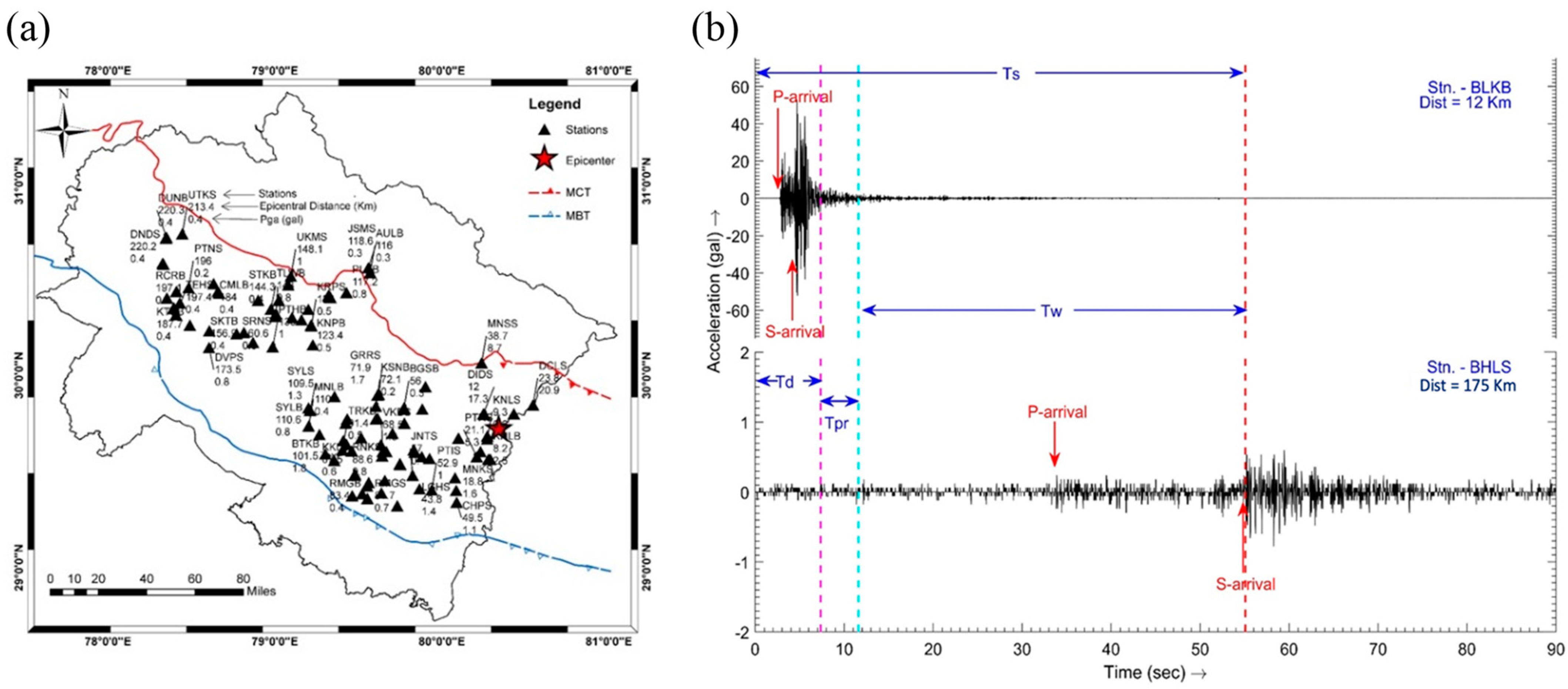
• The event was also recorded at 89 MEMS sensors and was detected within 11.61 s of the origin, taking only 4.26 s for processing, location and magnitude estimation, and warning dissemination. The quick estimation of magnitude using the amplitude data resulted in M_Pd 4.6; however, the moment tensor inversion resulted in M_w 5.2.
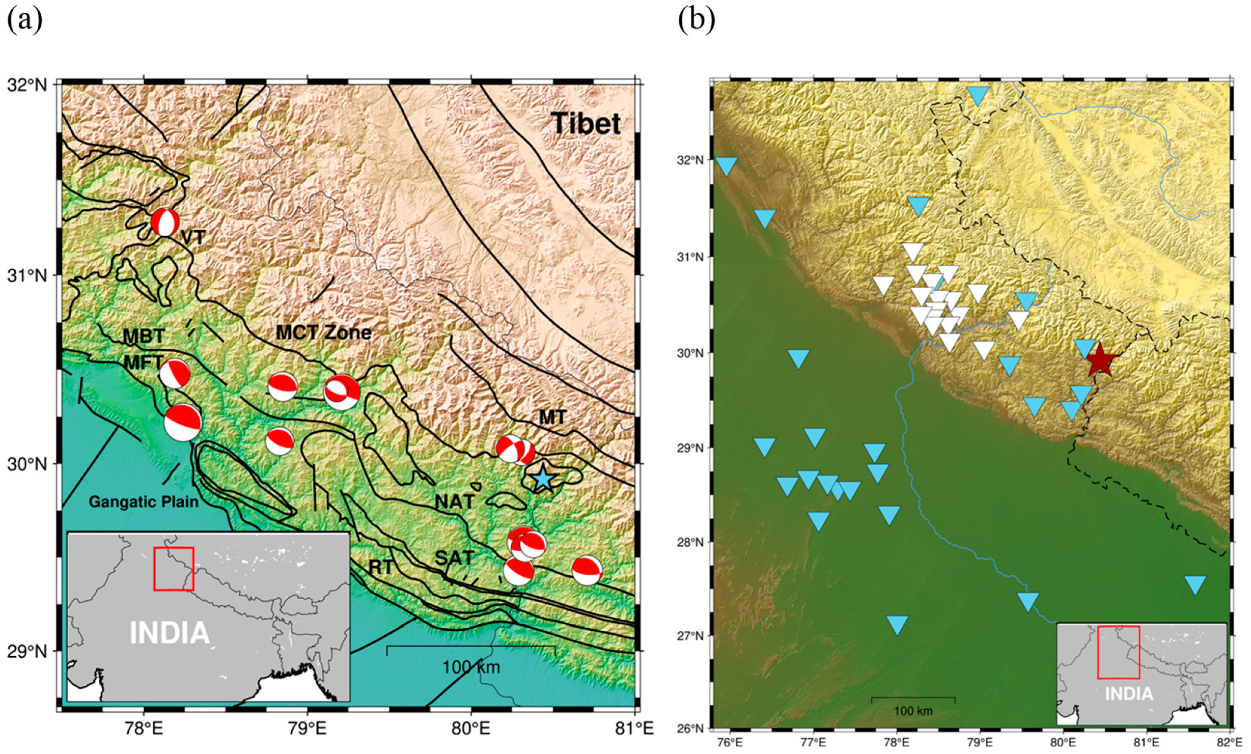
• The moment tensor inversion of the 11 May 2022 Dharchula earthquake using body and surface waves was performed. The moment tensor inversion solution was obtained using 30 broadband stations from both THDCIL (local) and NCS (regional) networks. The results revealed a thrust faulting rupture near the Chiplakot klippe. Additionally, the depth test in Figure 3c depicted that the depth corresponding to the minimum misfit was determined to be 2 km.
• The time shift plots reveal that the used 1D velocity model is slower than the actual crustal velocities. The negative time shifts in Figure 3 (and Figure S1) mean that the synthetics are arriving later and need to be shifted negatively in time in order to be matched with the observed.
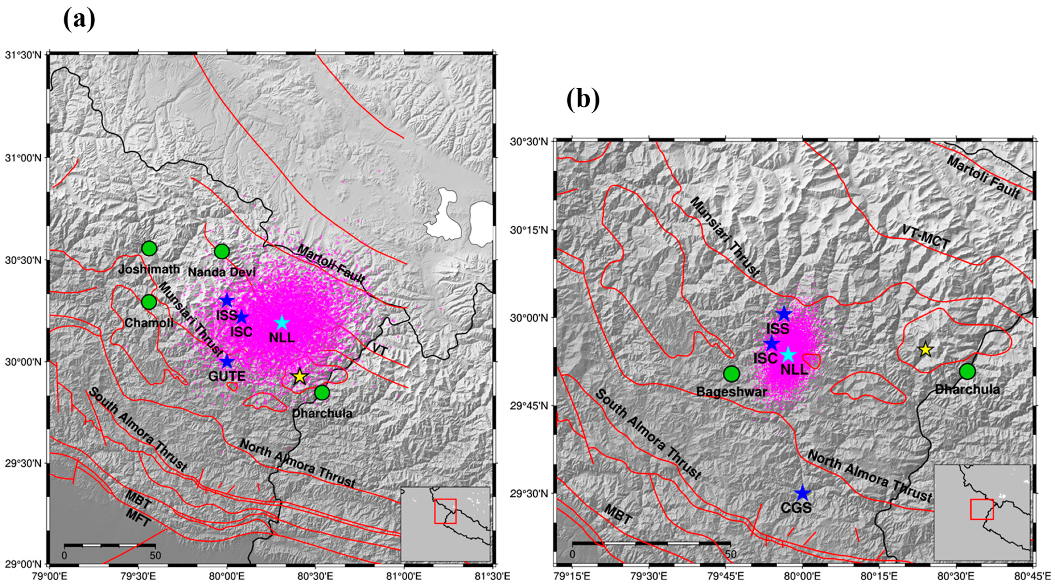
• We performed the relocation of two major historical events that occurred in the vicinity of the Dharchula event. The relocation resulted in the maximum likelihood locations of M_w 6.5, the 1945 Nanda Devi event, and M_w 6.3, the 1958 Kapkote event, which occurred at a depth around 20 km along the mid-crustal Himalayan.

There has not been a large earthquake in the central seismic gap region of the Himalayas since 1803. The accumulated stress in this region is accommodated by structural deformation and major earthquakes such as the 1945 and 1958 events. Whether the slip is accommodated aseismically in this region is yet to be identified. The impending large earthquake in this region mandates the well-functioning EEWS as showcased in this example. We also performed the source mechanism inversion and placed it in context with the past events that occurred in the vicinity. To improve the capability of EEWS, AI/ML techniques can further be adopted, and report dissemination can be expanded by including real-time estimation of moment tensor solutions.

6. Data and Resources

The waveform data are obtained from the Broadband Seismometer Network deployed in Garhwal Himalayas by the Department of Earthquake Engineering, IIT Roorkee, and the National Center of Seismology, New Delhi. The EEWS information and dataset used in this article are received from the EEWS Lab in the Centre of Excellence in Disaster Mitigation & Management, IIT Roorkee.

Travel-time data used for relocation for historical events are freely available from the International Seismological Center (http://www.isc.ac.uk/iscbulletin/search/catalogue/) accessed on 1 May 2022. The USGS catalog origin parameters were obtained from https://earthquake.usgs.gov/earthquakes/eventpage/us7000h8ii/executive (last accessed 1 December 2022). All the maps were drawn using the Python version of Generic Mapping Tool PyGMT (https://github.com/GenericMappingTools/pygmt, accessed on 1 December 2022) and inversion was conducted using MTUQ (https://github.com/uafgeotools/mtuq, accessed on 1 December 2022). The publicly available “BhuDEV” mobile app can also be downloaded by accessing the following links:

For Android users—https://play.google.com/store/apps/details?id=com.iitr.eews (accessed on 1 December 2022).

For iPhone users—https://apps.apple.com/in/app/11aetan/id1661902248 (accessed on 1 December 2022).

References

1. Patriat, P.; Achache, J. India-Eurasia collision chronology has implications for crustal shortening and driving mechanism of plates. Nature 1984, 311, 615–621. [Google Scholar] [CrossRef]
2. Molnar, P.; Topponnier, P. Cenozoic Tectonics of Asia: Effects of a Continental Collision. Science 1975, 189, 419–426. [Google Scholar] [CrossRef]
3. Bilham, R. Earthquakes in India and the Himalaya: Tectonics, geodesy and history. Ann. Geophys. 2004, 47, 839–858. [Google Scholar] [CrossRef]
4. Srivastava, H.N.; Verma, M.; Bansal, B.K.; Sutar, A.K. Discriminatory characteristics of seismic gaps in Himalaya. Geomat. Nat. Hazards Risk 2015, 6, 224–242. [Google Scholar] [CrossRef]
5. Kayal, J.R. Microearthquake activity in some parts of the Himalaya and the tectonic model. Tectonophysics 2001, 339, 331–351. [Google Scholar] [CrossRef]
6. Gautam, D. Unearthed lessons of 25 April 2015 Gorkha earthquake (MW 7.8): Geotechnical earthquake engineering perspectives. Geomat. Nat. Hazards Risk 2017, 8, 1358–1382. [Google Scholar] [CrossRef]
7. Wyss, M. Second Round of Evaluations of Proposed Earthquake Precursors. Pure Appl. Geophys. 1997, 149, 3–16. [Google Scholar] [CrossRef]
8. Chamoli, B.P.; Kumar, A.; Chen, D.Y.; Gairola, A.; Jakka, R.S.; Pandey, B.; Kumar, P.; Rathore, G. A Prototype Earthquake Early Warning System for Northern India. J. Earthq. Eng. 2021, 25, 2455–2473. [Google Scholar] [CrossRef]
9. Ekström, G.; Nettles, M.; Dziewoński, A.M. The global CMT project 2004–2010: Centroid-moment tensors for 13,017 earthquakes. Phys. Earth Planet. Inter. 2012, 200–201, 1–9. [Google Scholar] [CrossRef]
10. DasGupt, S.; Pandey, P.; Ganguly, D.; Iqbal, Z. Seismotectonic Atlas of India and Its Environs; Geological Survey of India: Kolkata, India, 2000. [Google Scholar]
11. Valdiya, K.S. Uplift and geomorphic rejuvenation of the Himalaya in the Quaternary period. Curr. Sci. 1993, 64, 873–885. [Google Scholar]
12. Paul, A.; Gupta, S.C.; Pant, C.C. CODA Q estimates for Kumaun Himalaya. Proc. Indian Acad. Sci. Earth Planet. Sci. 2003, 112, 569–576. [Google Scholar] [CrossRef]
13. Valdiya, K.S. Evolution of the Himalaya. In Lithosphere: Structure, Dynamics and Evolution; Naqvi, S.M., Gupta, H.K., Balakrishna, S., Eds.; Elsevier: Amsterdam, The Netherlands, 1984; Volume 105, pp. 229–248. [Google Scholar]
14. Kumar, P.; Kamal; Sharma, M.L.; Pratibha; Jakka, R.S.; Kumar, A.; Joshi, G.C.; Rautela, P. Successful Alert Issuance with Sufficient Lead Time by Uttarakhand State Earthquake Early Warning System: Case Study of Nepal Earthquakes. J. Geol. Soc. India 2023, 99, 303–310. [Google Scholar] [CrossRef]
15. Chen, D.Y.; Hsiao, N.C.; Wu, Y.M. The earthworm based earthquake alarm reporting system in Taiwan. Bull. Seismol. Soc. Am. 2015, 105, 568–579. [Google Scholar] [CrossRef]
16. Allen, R.V. Automatic Earthqauke Recognition and Timing From Single Traces. Bull. Seismol. Soc. Am. 1978, 68, 1521–1532. [Google Scholar] [CrossRef]
17. Allen, R. Automatic phase pickers: Their present use and future prospects. Bull. Seismol. Soc. Am. 1982, 72, S225–S242. [Google Scholar] [CrossRef]
18. Kanaujia, J.; Kumar, A.; Gupta, S.C. 1D velocity structure and characteristics of contemporary local seismicity around the Tehri region, Garhwal Himalaya. Bull. Seismol. Soc. Am. 2015, 105, 1852–1869. [Google Scholar] [CrossRef]
19. Geiger, L. Probability method for the determination of earthquake epicenters from the arrival times only. Bull. Saint Louis Univ. 1912, 8, 60–71. [Google Scholar]
20. Isacks, B.; Oliver, J.; Sykes, L.R. Seismology and New Global Tectonics. J. Geophys. Res. 1968, 73, 5855–5899. [Google Scholar] [CrossRef]
21. Eyre, T.S.; Van Der Baan, M. Overview of moment-tensor inversion of microseismic events. Lead. Edge 2015, 34, 882–888. [Google Scholar] [CrossRef]
22. da Silva, S.L.E.F.; Julià, J.; Bezerra, F.H.R. Deviatoric moment tensor solutions from spectral amplitudes in surface network recordings: Case study in São aetano, Pernambuco, Brazil. Bull. Seismol. Soc. Am. 2017, 107, 1495–1511. [Google Scholar] [CrossRef]
23. Zhu, L.; Helmberger, D.V. Advancement in source estimation techniques using broadband regional seismograms. Bull. Seismol. Soc. Am. 1996, 86, 1634–1641. [Google Scholar] [CrossRef]
24. Dreger, D.; Uhrhammer, R.; Pasyanos, M.; Franck, J.; Romanowicz, B. Regional and far-regional earthquake locations and source parameters using sparse broadband networks: A test on the Ridgecrest sequence. Bull. Seismol. Soc. Am. 1998, 88, 1353–1362. [Google Scholar] [CrossRef]
25. Silwal, V.; Tape, C. Seismic moment tensors and estimated uncertainties in southern Alaska. J. Geophys. Res. Solid Earth 2016, 121, 2772–2797. [Google Scholar] [CrossRef]
26. Beyreuther, M.; Barsch, R.; Krischer, L.; Megies, T.; Behr, Y.; Wassermann, J. ObsPy: A python toolbox for seismology. Seismol. Res. Lett. 2010, 81, 530–533. [Google Scholar] [CrossRef]
27. Zhu, L.; Rivera, L.A. A note on the dynamic and static displacements from a point source in multilayered media. Geophys. J. Int. 2002, 148, 619–627. [Google Scholar] [CrossRef]
28. Mahesh, P.; Rai, S.S.; Sivaram, K.; Paul, A.; Gupta, S.; Sarma, R.; Gaur, V.K. One-dimensional reference velocity model and precise locations of earthquake hypocenters in the Kumaon-Garhwal Himalaya. Bull. Seismol. Soc. Am. 2013, 103, 328–339. [Google Scholar] [CrossRef]
29. Silwal, V.; Tape, C.; Lomax, A. Crustal earthquakes in the Cook Inlet and Susitna region of southern Alaska. Tectonophysics 2018, 745, 245–263. [Google Scholar] [CrossRef]
30. Tape, W.; Tape, C. A geometric setting for moment tensors. Geophys. J. Int. 2012, 190, 476–498. [Google Scholar] [CrossRef]
31. Lomax, A.; Virieux, J.; Volant, P.; Berge-Thierry, C. Probabilistic earthquake location in 3D and layered models. In Advances in Seismic Event Location; Thurber, C.H., Rabinowitz, N., Eds.; Springer-Science+Business Media, B.V.: Berlin, Germany, 2000; ISBN 978-94-015-9536-0. [Google Scholar]
32. Kennett, B.L.N.; Engdahl, E.R.; Buland, R. Constraints on seismic velocities in the Earth from traveltimes. Geophys. J. Int. 1995, 122, 108–124. [Google Scholar] [CrossRef]
33. Crotwell, H.P.; Owens, T.J.; Ritsema, J. The TauP Tookit: Flexible Seismic Travel-time and Ray-path Utilities. Seismol. Res. Lett. 1999, 70, 154–160. [Google Scholar] [CrossRef]
34. Gutenberg, B.; Richter, C.F. Seismicity of the Earth and Associated Phenomena; Princeton University Press: Princeton, NJ, USA, 1958. [Google Scholar]
35. Jai, K.; Mittal, R.S.; Chandrasekaran, A.R.; Manglik, S.K. Kapkote Earthquake of Dec. 28, 1958; University of Roorkee: Roorkee, India, 1958. [Google Scholar]
36. Khattri, K.N. Great Earthquakes, Seismicity Gaps and Potential for Earthquake Disaster along the Himalaya Plate Boundary. Tectonophysics 1987, 138, 79–92. [Google Scholar] [CrossRef]
Figure 2. (a) Position of the 89 EEWS sensors where the event was recorded. The numbers below the stations’ names show the epicentral distance and estimated peak ground acceleration (gal). (b) Demonstrates warning time estimation, Tw = 43.48 s, for the BHLS site using information from the nearby station (BLKB). The diagram shows event detection time (Td), data processing time (Tpr), event reporting time (Tr), and shear wave travel time (Ts) at BHLS.
Geohazards 04 00029 g002
Figure 3. (a) Waveform fits for a subset of stations used for inversion. Moment tensor solution and waveform comparisons for the example event 2022051104331015. The first two columns represent the vertical and radial components of body waves; the next last three columns represent the vertical, radial, and transverse components of surface waves. See Silwal and Tape, 2016 for a detailed description of the figure and methodology [25]. (b) Moment tensor beachball for the minimum misfit solution. Triangles are marked only for stations for which the polarity information is used for inversion. A red downward triangle is marked when the observed polarity does not match the theoretical polarity. Blue downward triangles show stations with matched down-polarity, and green upward triangles for matched up-polarity. (c) Grid search for minimum misfit depth for the event is obtained at 2 km.
Geohazards 04 00029 g003
Figure 4. Posterior samples of hypocenter location (magenta dots) for (a) the 1945 Nanda Devi Earthquake (Mw 6.5) and (b) the 1958 Kapkote earthquake (Mw 6.3). The cyan star represents the maximum likelihood epicenter of the earthquake obtained using non-linear inversion (NLL) and blue stars represent the location obtained from other sources mentioned in the ISC database (ISC—International Seismological Center, GUTE: Gutenberg-Richter catalog; CGS: Coast and Geological Survey, USA; ISS: International Seismological Summary). Marked in red is the surface delineation of active faults [10] (MCT—Main Central Trust; MBT—Main Boundary Thrust; MFT—Main Frontal Thrust; VT—Vaikrita Thrust). Yellow marks the Dharchula event. (a) also shows the major structural features.
Geohazards 04 00029 g004