On Low Hubble Expansion Rate from Planck Data Anomalies

Abstract

From the linear perturbations of Nash–Greene fluctuations of a background metric, we obtain profiles of Hubble function evolution $H\left(z\right)$ and $f{\sigma }_8\left(z\right)$ measurements as compared with the $\mathrm{\Lambda }$CDM results at intermediate redshifts $0.1<z<1$. For parameter estimation, we use joint data from Planck Cosmic Microwave Background (CMB) likelihoods of CMB temperature and polarization angular power spectra, Barionic Acoustic Oscillations (BAO) and local measurements of Hubble constant $H_0$ from the Hubble Space Telescope (HST). We analyze the stability of the effective Newtonian constant $G_{eff}$ and its agreement with Big Bang Nucleosynthesis (BBN) constraints. We show that our results are highly compatible with the $\mathrm{\Lambda }$CDM paradigm, rather extending the perspective for further studies on redshift-space galaxy clustering data. Moreover, we obtain the CMB TT angular spectra with the Integrated Sachs–Wolfe (ISW) effect, which is weakened on low-l scales. The resulting linear matter power spectrum $P\left(k\right)$ profile is also compatible with $\mathrm{\Lambda }$CDM results but somewhat degenerate with an early dark energy (DE) contribution. Finally, posing a dilemma to the solution of Hubble tension, our results indicate a low Hubble expansion rate suggesting possible anomalies in Planck data in consonance with the recent South Pole Telescope (SPT-3G) data.

1. Introduction

The $\mathrm{\Lambda }$CDM model is regarded as the standard cosmological model. It is the most successful simpler solution to tackle the problem of the accelerated expansion of the universe [1,2,3,4,5,6,7,8,9,10,11] with agreement with larger events of the data collected to date [1]. On the other hand, it lacks fundamental theoretical grounds on explaining the unknown nature of the cosmological constant $\mathrm{\Lambda }$ and the (Cold) Dark Matter (CDM) [12,13,14,15,16,17,18]. The fact that the underlying nature of these components are still unknown, it brought forth a plethora of competing cosmological models. In this direction, apart from $\mathrm{\Lambda }$CDM paradigm, in this paper, based on previous works [19,20,21], we explore the possibility to add a new curvature to General Relativity (GR) and to analyze the physical implications of such a mechanism. In this framework, gravity naturally accesses extra-dimensions that are no longer an ad hoc proposition. Then, it opens a possible direction for tackling the fundamental problem of the large difference of the ratio of the Planck masses ($M_{Pl}$) to the electroweak energy scale $M_{EW}$ in such $M_{Pl}/M_{EW}\sim {10}^{16}$, the so-called problem of unification of fundamental interactions. The sought-after solution to such a problem spawned a whole arena of multidimensional models such as Kaluza–Klein or/and string inspired as the works of the Arkani-Hamed, Dvali and Dimopolous [22], for short, ADD model, the Randall–Sundrum model [23,24], the Dvali–Gabadadze–Porrati model (DPG) [25] and variants. Differently from these brane/string inspired models, we adopt the embedding of geometries as a cornerstone for elaborating a gravitational model, as proposed in several independent investigations [19,20,21,26,27,28,29,30,31,32,33,34,35,36,37,38,39]. In this work, we use the resulting linear cosmological perturbation equations to test our model [40,41,42,43] mainly in ref. [44] analyzing Hubble function evolution $H\left(z\right)$ and $f{\sigma }_8\left(z\right)$ measurements and the stability of the effective Newtonian constant $G_{eff}$ that carries a signature of the extrinsic curvature, the key object in our framework. In particular, the quantity $f{\sigma }_8\left(z\right)$ is defined in terms of ${\sigma }_8$ parameter that is the RMS amplitude of matter density at a scale of a radius $R\sim 8$h.Mpc${}^{-1}$ within an enclosed mass of a sphere [45].

The outline of the paper is organized in sections. In Section 1, we revise the embedding of geometries and how it may be used to construct a physical model. In this context, the Nash–Greene theorem is discussed. The second and third sections verse on the obtainment of the Hubble evolution $H\left(z\right)$ from the background Friedmann–Lemaître–Robertson–Walker (FLRW) metric and cosmological scalar perturbation equations in Newtonian gauge, respectively. In the fourth section, we analyze the stability of $G_{eff}$ and the evolution of $H\left(z\right)$ and $f{\sigma }_8\left(z\right)$. To constrain the parameters, we use a parameter estimator MontePhyton [46,47,48] sampler associated with the module classy in the Cosmic Linear Anisotropy Solving System CLASS [49,50,51]. We perform a joint data analysis applying the Markov Chain Monte Carlo (MCMC) sample technique from Planck CMB likelihoods [1] of temperature and polarization angular power spectra (high-l.TT+high-l.plik.TTTEEE + low-l EE polarization+ low-l TT temperature), BAO data by the public available likelihoods at https://doi.org/github.com/brinckmann/montepython_public (accessed on 10 October 2022 ) extracted from 6dFGS [52], BOSS DR10&11: LOWZ, CMASS [53], SDSS DR7: MGS [54] and BOSS DR12: BAO LOWZ&CMASS [55], including $f{\sigma }_8$ measurements. We also consider local measurements of $H_0$ from the Hubble Space Telescope (HST) [56]. In addition, we compare our results with the $\mathrm{\Lambda }$CDM model in $f{\sigma }_8\left(z\right)$ measurements using the data points of SDSS [57,58,59], 6dFGS [60], IRAS [61,62], 2MASS [61,63], 2dFGRS [64], GAMA [65], BOSS [66], WiggleZ [67], Vipers [68], FastSound [69], BOSS Q [70] and additional points from the 2018 SDSS-IV [71,72,73,74]. For the background evolution of Hubble function $H\left(z\right)$, we use data points from [75,76] and some “clustering” measurements of $H\left(z\right)$[77]. Moreover, an analysis of the unlensed CMB TT power spectrum and the linear matter power $P\left(k\right)$ is performed. In the final section, we present our remarks and prospects. We adopt the Landau time-like convention $(---+)$ for the signature of the four-dimensional embedded metric and speed of light $c=1$. Concerning notation, capital Latin indices run from 1 to 5. Small case Latin indices refer only to the one extra-dimension considered. All Greek indices refer to the embedded space–time counting from 1 to 4. From here on, we indicate the non-perturbed (background) quantities by the upper-script symbol “0”.

2. The Induced Four–Dimensional Equations in an Embedded Space–Time

We define a model endowed with a gravitational action S in the presence of confined matter fields on a four-dimensional embedded space–time embedded in a five-dimensional one as

$$S=-\frac{1}{2{\kappa }_5^2}\int {\sqrt{\left|\mathcal{G}\right|}}^5\mathcal{R}{d}^{5}x-\int \sqrt{\left|\mathcal{G}\right|}{\mathcal{L}}_m^{*}{d}^{5}x,$$

(1)

where ${\kappa }_5^2$ is a fundamental energy scale on the embedded space, ${}^5\mathcal{R}$ denotes the five-dimensional Ricci scalar of the bulk and ${\mathcal{L}}_m^{*}$ denotes the confined matter content. Such a Lagrangian contains the matter energy momentum tensor that fulfills a finite hypervolume with constant radius l along the fifth dimension.

The variation of Einstein–Hilbert action in Equation (1) with respect to the bulk metric ${\mathcal{G}}_{AB}$ leads to the higher-dimensional Einstein equations

$${}^5{\mathcal{R}}_{AB}-\frac{1}{2}{\mathcal{G}}_{AB}={\alpha }^{*}{\mathcal{T}}_{AB},$$

(2)

where ${\alpha }^{*}$ is the energy scale parameter and ${\mathcal{T}}_{AB}$ is the energy–momentum tensor for the bulk [19,20,21,30] and the five-dimensional bulk with constant curvature whose related Riemann tensor is

$${}^5{\mathcal{R}}_{ABCD}=K_{*}\left({\mathcal{G}}_{AC}{\mathcal{G}}_{BD}-{\mathcal{G}}_{AD}{\mathcal{G}}_{BC}\right),A...D=1...5,$$

where ${\mathcal{G}}_{AB}$ denotes the bulk metric components in arbitrary coordinates and the constant curvature $K_{*}$ is either zero (flat bulk) or it can have positive (deSitter) or negative (anti-deSitter) constant curvatures. In accordance with observations of Planck collaboration [1], they indicate a very small value of the cosmological constant $\mathrm{\Lambda }$; in this work, we ignore any contribution of such quantity to cosmic dynamics. As a result, we chose $K_{*}=0$, although any other choice of $K_{*}$ may be possible.

The bulk geometry is actually defined by the Einstein–Hilbert principle in Equation (1), which leads to Einstein’s equations, as shown in Equation (2). The confinement condition [78,79] on these equations implies that $K_{*}={\mathrm{\Lambda }}_{*}/6=0$. Thus, the confined components of the bulk–energy tensor ${\mathcal{T}}_{AB}$ are proportional to the energy–momentum tensor of standard General Relativity (GR), i.e., ${\alpha }_{*}{T}_{\mu \nu }=8\pi G{T}_{\mu \nu }$, where G is the gravitational Newtonian constant. The confinement implies that we are restricted to the four-dimensionality of the space–time. This is reinforced by the experimentally consistent Yang–Mills structures of gauge fields that are valid only in four dimensions [80], even though theoretical extensions are possible in the context of branes and strings. Hence, only gravity propagates in the bulk space, and the vector and scalar components of bulk energy tensor are zero, i.e., $T_{\mu a}=0$ and $T_{ab}=0$, respectively.

In this work, the mathematical background of the theoretical embedding structure is well oriented by the Nash–Greene theorem [81,82]. Such a theorem states that a complete embedding between pseudo-Riemannian manifolds results from a differentiable mapping between the functions of the related manifolds to guarantee that the embedded geometry and its deformations will be differentiable. Moreover, the bulk metric must obey the Einstein–Hilbert principle. Differently from rigid embedding models, where the perturbed bulk equations are a must, e.g., [23,24,25], Nash–Greene mechanism simplifies the evolution of the perturbed cosmological equations. Once the dynamical embedding is fully set, we do not need to perturb the bulk geometry since the perturbations on the embedded space–time were already triggered, and vice-versa. Although embedding can be made in an arbitrary number of dimensions (see [19,20,21,29,30,33,34,35,36,38,39]), the current alternative models of gravitation are normally stated in five dimensions at most.

Next, we summarize the embedding process to obtain the induced gravitational equations from the bulk on the embedded space–time. First, a Riemannian manifold $V_4$ is endowed with a non-perturbed metric ${}^{\left(0\right)}{g}_{\mu \nu }$ which is locally and isometrically embedded in a five-dimensional Riemannian manifold $V_5$. Hence, a differentiable and regular map can be defined as $\mathcal{X}:V_4\to V_5$, which leads to

$$\begin{array}{ccc}\hfill {\mathcal{X}}_{,\alpha }^A{\mathcal{X}}_{,\beta }^B{\mathcal{G}}_{AB}& =& {}^{\left(0\right)}{g}_{\alpha \beta },\hfill \end{array}$$

(3)

$$\begin{array}{ccc}\hfill {\mathcal{X}}_{,\alpha }^A{}^0{\eta }_a^B{\mathcal{G}}_{AB}& =& 0,\hfill \end{array}$$

(4)

$$\begin{array}{ccc}\hfill {}^0{\eta }_a^A{}^0{\eta }_b^B{\mathcal{G}}_{AB}& =& 1,\hfill \end{array}$$

(5)

where the colons denote ordinary derivatives, ${\mathcal{X}}^A$ is the non-perturbed embedding coordinate, ${\mathcal{G}}_{AB}$ is the metric components of $V_5$ in arbitrary coordinates and ${}^0\eta$ denotes the non-perturbed unit vector field orthogonal to $V_4$. The preferred orthogonal direction for perturbations avoids possible coordinate gauges which may produce false perturbations. Moreover, the set of Equations (3)–(5) represents the isometry, orthogonality and normalization conditions. Their integration gives the embedding map $\mathcal{X}$.

In this framework, it marks the appearance of a new curvature element that is the extrinsic curvature. As commonly defined in traditional textbooks [83], the non-perturbed extrinsic curvature $k_{\mu \nu }^{\left(0\right)}$ is given by

$$k_{\mu \nu }^{\left(0\right)}=-{\mathcal{X}}_{,\mu }^A{}^0{\eta }_{,\nu }^B{\mathcal{G}}_{AB}={\mathcal{X}}_{,\mu \nu }^A{}^0{\eta }^B{\mathcal{G}}_{AB}.$$

(6)

which is the projection of the variation of the vector ${}^0\eta$ onto the tangent plane. It plays an essential role in the embedding process and may inflict relevant consequences in terms of elaboration of a physical model.

Any geometric object $\overline{\Omega }$ can be constructed in the embedded space $V_4$ at any orthogonal direction ${}^0\eta$ by $\Omega =\overline{\Omega }+\delta y{\pounds }_{{}^0\eta }\overline{\Omega }$ that is the Lie transport ${\pounds }_{{}^0\eta }$ along the flow at certain small distances $\delta y$. It is worth noting that it is irrelevant if the distances $\delta y$ are time-like or not, nor if they are positive or negative. Thus, the Lie transport of the Gaussian coordinates’ vielbein $\left\{{\mathcal{X}}_{\mu }^A{,}^0{\eta }_a^A\right\}$ in $V_4$ leads to a new perturbed vielbein coordinates $\left\{{\mathcal{Z}}_{\mu }^A{,}^0{\eta }_a^A\right\}$ as

$$\begin{array}{ccc}\hfill {\mathcal{Z}}_{,\mu }^A& =& {\mathcal{X}}_{,\mu }^A+\delta y{\pounds }_{{}^0\eta {\mathcal{X}}_{,\mu }^A}={\mathcal{X}}_{,\mu }^A+\delta y{}^0{\eta }_{,\mu }^A,\hfill \end{array}$$

(7)

$$\begin{array}{ccc}\hfill {\eta }^A& =& {}^0{\eta }^A+\delta y{{[}^0\eta {,}^0\eta ]}^A={}^0{\eta }^A.\hfill \end{array}$$

(8)

From Equation (8), it is straightforward to check that the derivative of ${}^0\eta$ is not affected by perturbations in a sense that ${\eta }_{,\mu }\ne {}^0{\eta }_{,\mu }$. Likewise, from the non-perturbed case in Equations (3)–(5), one obtains a set of perturbed coordinates ${\mathcal{Z}}^A$ as

$${\mathcal{Z}}_{,\mu }^A{\mathcal{Z}}_{,\nu }^B{\mathcal{G}}_{AB}=g_{\mu \nu },{\mathcal{Z}}_{,\mu }^A{\eta }^B{\mathcal{G}}_{AB}=0,{\eta }^A{\eta }^B{\mathcal{G}}_{AB}=1.$$

(9)

Now, the perturbed coordinate $\mathcal{Z}$ defines a coordinate chart between the bulk and the embedded space–time which may evolve dynamically inside the bulk. Replacing Equations (7) and (8) in Equations (6) and (9), one obtains the set of both perturbed metric $g_{\mu \nu }$ and extrinsic curvature $k_{\mu \nu }$ in linear perturbation as

$$\begin{array}{ccc}& & g_{\mu \nu }=g_{\mu \nu }^{\left(0\right)}+\delta g_{\mu \nu }+...=g_{\mu \nu }^{\left(0\right)}-2y{k}_{\mu \nu }^{\left(0\right)}+...,\hfill \end{array}$$

(10)

$$\begin{array}{ccc}& & k_{\mu \nu }=k_{\mu \nu }^{\left(0\right)}+\delta k_{\mu \nu }+...=k_{\mu \nu }^{\left(0\right)}-2y{}^0{g}^{\rho \sigma }{k}_{\mu \rho }^{\left(0\right)}{k}_{\nu \sigma }^{\left(0\right)}+...\hfill \end{array}$$

(11)

As a result, we simply obtain the Nash deformation formula by the derivative of Equation (10) with respect to the y coordinate given by

$$k_{\mu \nu }^{\left(0\right)}=-\frac{1}{2}\frac{\partial g_{\mu \nu }^{\left(0\right)}}{\partial y}.$$

(12)

In the context of ADM formulation of GR, a suchlike formula was obtained by Choquet-Bruhat and J. York [84]. Differently from the Choquet-Bruhat–York condition, the concept of the y parameter is not restricted to be a time component. Moreover, Equation (12) justifies how the deformation parameter y does not explicitly appear in the line element $ds$ once the perturbation is virtually triggered in the embedding process. It also holds true for any perturbations resulting from n-parameter families of embedded submanifolds extended to a larger set of $y^a$. This notable feature is exclusive of embedding geometries with dynamical embeddings. Due to the fact that the dynamics of extrinsic curvature is commonly replaced by additional assumptions, the deformation parameter y is carried out in the metrics of rigid embedding models [23,24] to guarantee that perturbations can happen.

A final aspect of the Nash–Greene embeddings follows the logic that the evolution of the bulk induces the dynamics of the embedded space–time and vice-versa. Then, the comprehension of integrability equations is a sufficient and necessary condition. They are given by the non-trivial components of the Riemann tensor of the embedding space–time, namely Gauss and Codazzi equations, respectively, as

$$\begin{array}{ccc}& & {}^5{\mathcal{R}}_{ABCD}{\mathcal{Z}}^A{}_{,\alpha }{\mathcal{Z}}^B{}_{,\beta }{\mathcal{Z}}^C{}_{,\gamma }{\mathcal{Z}}^D{}_{,\delta }=R_{\alpha \beta \gamma \delta }+{(}^0{k}_{\alpha \gamma }{}^0{k}_{\beta \delta }-{}^0{k}_{\alpha \delta }{}^0{k}_{\beta \gamma }),\hfill \end{array}$$

(13)

$$\begin{array}{ccc}& & {}^5{\mathcal{R}}_{ABCD}{\mathcal{Z}}^A{}_{,\alpha }{\mathcal{Z}}^B{}_{,\beta }{\mathcal{Z}}^C{}_{,\gamma }{\eta }^D={}^0{k}_{\alpha [\beta ;\gamma ]},\hfill \end{array}$$

(14)

where ${}^5{\mathcal{R}}_{ABCD}$ is the five-dimensional Riemann tensor. The semicolon denotes the covariant derivative with respect to the metric, and the brackets apply the covariant derivatives to the adjoining indices only. By the relation in Equation (12), Nash proposes a solution for the long-standing problem of these equations due to their strong non-linearity. As a result, we can write in embedded vielbein $\{{\mathcal{Z}}_{,\mu }^A,{\eta }^A\}$ for the metric of the bulk in the vicinity of $V_4$ simply as

$$\begin{array}{ccc}\hfill {\mathcal{G}}_{AB}& =& \left(\begin{array}{cc}{g}_{\mu \nu }^{\left(0\right)}& 0\\ 0& 1\end{array}\right).\hfill \end{array}$$

(15)

3. Embedded Four-Dimensional FLRW Cosmology

In this section, we summarize some results of previous works [20,30,44] showing the main relations to obtain the Friedmann equation. The basic familiar line element of the FLRW four-dimensional metric is given by

$$d{s}^2=d{t}^2-a^2\left(d{r}^2+r^{2}d{\theta }^2+r^2{sin}^2\theta d{\varphi }^2\right),$$

(16)

where the expansion factor is denoted by $a\equiv a\left(t\right)$. The coordinate t denotes the physical time. In the Newtonian frame, the former equations turns out to be

$$d{s}^2=d{t}^2-a^2\left(d{x}^2+d{y}^2+d{z}^2\right).$$

(17)

Using Equations (2), (15) and (17), we can obtain the non-perturbed field equations of induced field equations from a five-dimensional bulk as

$$\begin{array}{ccc}\hfill G_{\mu \nu }^{\left(0\right)}+Q_{\mu \nu }^{\left(0\right)}& =& 8\pi G{T}_{\mu \nu }^{\left(0\right)},\hfill \end{array}$$

(18)

$$\begin{array}{ccc}\hfill k_{\mu [\nu ;\rho ]}^{\left(0\right)}& =& 0,\hfill \end{array}$$

(19)

where the energy–momentum tensor of the confined perfect fluid is denoted by $T_{\mu \nu }^{\left(0\right)}$ and G is the gravitational Newtonian constant. Here, $G_{\mu \nu }^{\left(0\right)}$ denotes the four-dimensional Einstein tensor and $Q_{\mu \nu }^{\left(0\right)}$ is called deformation tensor.

The non-perturbed extrinsic term $Q_{\mu \nu }^{\left(0\right)}$ in Equation (19) is given by

$$Q_{\mu \nu }^{\left(0\right)}=k_{\mu }^{\left(0\right)\rho }{k}_{\rho \nu }^{\left(0\right)}-k_{\mu \nu }^{\left(0\right)}h-\frac{1}{2}\left(K^2-h^2\right)g_{\mu \nu }^{\left(0\right)},$$

(20)

where we denote the mean curvature by $h^2=h·h$ and $h={}^0{g}^{\mu \nu }{}^0{k}_{\mu \nu }$ and the Gaussian curvature by $K^2=k^{\mu \nu \left(0\right)}{k}_{\mu \nu }^{\left(0\right)}$ . By direct derivation, Equation (20) is conserved as

$$Q_{\mu \nu ;\mu }^{\left(0\right)}=0.$$

(21)

The deformation equation in Equation (19) was firstly introduced in refs. [19,20,21].

Since the extrinsic curvature is diagonal in FLRW space–time, one finds their components using Equation (19), which can be split into spatial and time parts as

$$k_{ij,k}^{\left(0\right)}-{\Gamma }_{ik}^a{k}_{aj}^{\left(0\right)}=k_{ik,j}^{\left(0\right)}-{\Gamma }_{ij}^a{k}_{ak}^{\left(0\right)}.$$

(22)

In the Newtonian frame, the spatial components are also symmetric and, from Equation (22), one can obtain $k_{11}^{\left(0\right)}=k_{22}^{\left(0\right)}=k_{33}^{\left(0\right)}=b\equiv b\left(t\right)$ and

$$\begin{array}{c}\hfill k_{ij}^{\left(0\right)}=\frac{b}{a^2}{g}_{ij},i,j=1,2,3,k_{44}^{\left(0\right)}=\frac{-1}{\dot{a}}\frac{d}{dt}\frac{b}{a}.\end{array}$$

(23)

The set of the following objects can be found as

$$\begin{array}{ccc}\hfill & & k_{44}^{\left(0\right)}=-\frac{b}{a^2}\left(\frac{B}{H}-1\right),\hfill \end{array}$$

(24)

$$\begin{array}{ccc}& & K^2=\frac{b^2}{a^4}\left(\frac{B^2}{H^2}-2\frac{B}{H}+4\right),h=\frac{b}{a^2}\left(\frac{B}{H}+2\right),\hfill \end{array}$$

(25)

$$\begin{array}{ccc}& & Q_{ij}^{\left(0\right)}=\frac{b^2}{a^4}\left(2\frac{B}{H}-1\right)g_{ij}^{\left(0\right)},Q_{44}^{\left(0\right)}=-\frac{3b^2}{a^4},\hfill \end{array}$$

(26)

$$\begin{array}{ccc}& & Q^{\left(0\right)}=-(K^2-h^2)=\frac{6b^2}{a^4}\frac{B}{H},\hfill \end{array}$$

(27)

where the Hubble parameter is defined as $H\equiv H\left(t\right)=\frac{\dot{a}}{a}$. The function $B=B\left(t\right)\equiv \frac{\dot{b}}{b}$ is defined as in analogy with the Hubble parameter. As shown in detail in ref. [44], the bending function $b\left(t\right)$ is given by

$$b\left(t\right)=b_{0}a{\left(t\right)}^{{\beta }_0},$$

(28)

that solves univocally the set of the components of the extrinsic curvature in Equation (23).

The hydrodynamical equations are obtained in a very standard fashion. We start with a non-perturbed stress–energy tensor in a co-moving fluid that is defined as

$$T_{\mu \nu }^{\left(0\right)}=\left({\rho }^{\left(0\right)}+p^{\left(0\right)}\right)u_{\mu }{u}_{\nu }-p^{\left(0\right)}{g}_{\mu \nu }^{\left(0\right)};u_{\mu }={\delta }_{\mu }^4,$$

and its immediate conservation $T_{\mu \nu ;\mu }^{\left(0\right)}=0$ that leads to the equation

$${\rho }^{\left(0\right)}+3H\left({\rho }^{\left(0\right)}+p^{\left(0\right)}\right)=0.$$

(29)

Hence, one obtains the following Friedmann equation as

$$H^2=\frac{8}{3}\pi G{\rho }^{\left(0\right)}+\frac{b^2}{a^4},$$

(30)

where ${\rho }^{\left(0\right)}$ is the present value of the non-perturbed matter density (${\rho }^{\left(0\right)}\equiv {\rho }_m^{\left(0\right)}\left(t\right)$). For a pressureless fluid, one obtains the matter density in terms of redshift as

$${\rho }_m^{\left(0\right)}\left(t\right)={\rho }_{m\left(0\right)}^{\left(0\right)}{a}^{-3}={\rho }_{m\left(0\right)}^{\left(0\right)}{(1+z)}^3.$$

Likewise, one writes Equation (30) simply as

$$H^2=\frac{8}{3}\pi G{\rho }_{m\left(0\right)}^{\left(0\right)}{(1+z)}^3+b_0^2{(1+z)}^{4-2{\beta }_0}.$$

(31)

Using the standard definition of the cosmological parameter ${\Omega }_i=\frac{8\pi G}{3H_0^2}{\rho }_{i\left(0\right)}^{\left(0\right)}$, one obtains

$${\left(\frac{H}{H_0}\right)}^2={\Omega }_{m\left(0\right)}{(1+z)}^3+(1-{\Omega }_{m\left(0\right)}){(1+z)}^{4-2{\beta }_0},$$

(32)

where ${\Omega }_{m\left(0\right)}$ is the current cosmological parameter for the matter content and for a flat universe ${\Omega }_{ext\left(0\right)}=1-{\Omega }_{m\left(0\right)}$, and $H_0$ is the current value of Hubble constant in units of km.s${}^{-1}$ Mpc${}^{-1}$. It is worth noting that Equation (32) with the ${\beta }_0$-parameter nearly resembles the wCDM model in terms of comparison with their Friedmann equations at background level, where w is a dimensionless parameter of the fluid equation of state $w=\frac{p}{\rho }$ [85]. It allows us to propose an effective “extrinsic fluid parameter” $w_{ext}$ with a fluid analogy by an effective Equation of State (EoS) as

$$w_{ext}=-1+\frac{1}{3}\left(4-2{\beta }_0\right).$$

(33)

From the dimensionless parameter ${\beta }_0$ with the dark energy fluid parameter w, we have ${\beta }_0=2-\frac{3}{2}\left(1+w\right)$, or equivalently, $w=-1-\frac{1}{3}\left(2{\beta }_0-4\right)$. Thus, one obtains $w_{ext}=w$. Hence, the dimensionless Hubble parameter $E\left(z\right)$ is given by

$$E^2\left(z\right)={\Omega }_{m\left(0\right)}{(1+z)}^3+\left(1-{\Omega }_{m\left(0\right)}\right){(1+z)}^{3(1+w)}.$$

(34)

which mimics a wCDM behavior at background level for $w\ne -1$. On the other hand, at perturbation level, differently from the $\mathrm{\Lambda }$CDM and wCDM models, our model provides an effective Newtonian constant $G_{eff}$ [44].

4. Scalar Perturbations in Newtonian Gauge

In longitudinal conformal Newtonian gauge, we use the standard element line as

$$d{s}^2=a^2[(1+2\mathrm{\Phi })d{\eta }^2-\left((1-2\mathrm{\Psi }){\delta }_{ij}d{x}^{i}d{x}^j\right],$$

(35)

where $\mathrm{\Phi }=\mathrm{\Phi }(\overrightarrow{x},\eta )$, and $\mathrm{\Psi }=\mathrm{\Psi }(\overrightarrow{x},\eta )$ denotes the Newtonian potential and the Newtonian curvature. As shown in detail in ref. [44], the resulting perturbed gravitational equations are written as

$$\begin{array}{ccc}\hfill \delta G_{\nu }^{\mu }& =& 8\pi G\delta T_{\nu }^{\mu }-\delta Q_{\nu }^{\mu },\hfill \end{array}$$

(36)

$$\begin{array}{ccc}\hfill \delta k_{\mu \nu ;\rho }& =& \delta k_{\mu \rho ;\nu }.\hfill \end{array}$$

(37)

Using the Nash–Greene theorem, we notice that Codazzi equations from Equation (37) do not propagate perturbations. It can be shown by calculating the linear perturbations generating a new geometry ${\tilde{g}}_{\mu \nu }=g_{\mu \nu }^{\left(0\right)}+\delta g_{\mu \nu }$ by Nash’s fluctuations. Then, the perturbed geometry is given by

$${\tilde{g}}_{\mu \nu }=g_{\mu \nu }^{\left(0\right)}-2\delta y{k}_{\mu \nu }^{\left(0\right)},$$

(38)

and the related perturbed extrinsic curvature is

$${\tilde{k}}_{\mu \nu }=k_{\mu \nu }^{\left(0\right)}-2\delta y{}^{\left(0\right)}{g}^{\sigma \rho }{k}_{\mu \sigma }^{\left(0\right)}{k}_{\nu \rho }^{\left(0\right)},$$

(39)

where we can identify $\delta k_{\mu \nu }={}^{\left(0\right)}{g}^{\sigma \rho }{k}_{\mu \sigma }^{\left(0\right)}{k}_{\nu \rho }^{\left(0\right)}$ and, using the Nash relation $\delta g_{\mu \nu }=-2k_{\mu \nu }^{\left(0\right)}\delta y$, we obtain

$$\delta k_{\mu \nu }={}^{\left(0\right)}{g}^{\sigma \rho }{k}_{\mu \sigma }^{\left(0\right)}\delta g_{\nu \rho }.$$

(40)

Applying Equation (40) to Equation (37), one obtains the same background equation in Equation (19). On the other hand, the perturbation of the deformation tensor $Q_{\mu \nu }$ is straightforward obtained as

$$\delta Q_{\mu \nu }=-\frac{3}{2}(K^2-h^2)\delta g_{\mu \nu }.$$

(41)

Consequently, the set of perturbed equations for a perturbed fluid with pressure p and density $\rho$ in Fourier space (with subscript “k”) is given by

$$\begin{array}{ccc}& & k^2{\mathrm{\Psi }}_k+3\mathcal{H}\left({\mathrm{\Psi }}_k^{{}^{\prime }}+{\mathrm{\Phi }}_k\mathcal{H}\right)=-4\pi G{a}^2\delta {\rho }_k+\chi \left(a\right){\mathrm{\Phi }}_k,\hfill \end{array}$$

(42)

$$\begin{array}{ccc}& & {\mathrm{\Psi }}_k^{{}^{\prime }}+\mathcal{H}{\mathrm{\Phi }}_k=-4\pi G{a}^2({\rho }_0+p_0)\theta ,\hfill \end{array}$$

(43)

$$\begin{array}{ccc}& & {\mathcal{D}}_k-\frac{1}{2}{\widehat{k}}^i·{\widehat{k}}_i({\mathrm{\Psi }}_k-{\mathrm{\Phi }}_k)=4\pi G{a}^2\delta p+9{\gamma }_0{k}^2{a}^{2{\beta }_0}{\mathrm{\Psi }}_k,\hfill \end{array}$$

(44)

where $\theta =i{k}^j\delta u_{\Vert j}$ denotes the divergence of fluid velocity in k-space, and, in the last previous equation, ${\mathcal{D}}_k$ denotes ${\mathcal{D}}_k={\mathrm{\Psi }}_k^{{}^{″}}+\mathcal{H}{(2{\mathrm{\Psi }}_k+{\mathrm{\Phi }}_k)}^{\prime }+({\mathcal{H}}^2+2{\mathcal{H}}^{\prime }){\mathrm{\Phi }}_k+\frac{1}{2}{k}^2({\mathrm{\Psi }}_k-{\mathrm{\Phi }}_k)$. Moreover, neglecting neither anisotropic stresses nor any fluid pressure, one obtains

$$k^2{\mathrm{\Phi }}_k+3\mathcal{H}\left({\mathrm{\Phi }}_k^{{}^{\prime }}+{\mathrm{\Phi }}_k\mathcal{H}\right)=-4\pi G{a}^2\delta {\rho }_k+9{\gamma }_0{k}^2{a}^{2{\beta }_0}{\mathrm{\Phi }}_k,$$

(45)

where the closure condition $\mathrm{\Psi }=\mathrm{\Phi }$ applies. In the subhorizon approximation with $k^2\gg {\mathcal{H}}^2$ or $k^2\gg a^2{H}^2$ as ${\mathrm{\Phi }}_k^{″},\mathcal{H}{\mathrm{\Phi }}_k^{\prime }\sim 0$, the “contrast” matter density ${\delta }_m\equiv \frac{\delta \rho }{{\rho }_0}$ is related to the potential ${\mathrm{\Phi }}_k$ by means of

$$k^2{\mathrm{\Phi }}_k=-4\pi G_{eff}{a}^2{\rho }_0{\delta }_m,$$

(46)

where $G_{eff}$ is the effective Newtonian constant that is given by

$$G_{eff}\left(a\right)=\frac{G}{1-9{\gamma }_0{a}^{1-3w}}.$$

(47)

The present form of Equation (47) results in a “flat” $G_{eff}$ once $G_{eff}$ is k-scale-independent, like that of $f\left(T\right)$ models [86,87]. Hereon, the present model is denoted as $\beta$-model only to facilitate the referencing. The parameter ${\gamma }_0$ is given by ${\gamma }_0={\beta }_0{b}_0^2$. Moreover, the extrinsic cosmological parameter ${\Omega }_{ext\left(0\right)}$ is written using a fluid analogy such as

$${\Omega }_{ext\left(0\right)}=\frac{8\pi G}{3H_0^2}{\rho }_{ext\left(0\right)}^{\left(0\right)}\equiv \frac{b_0^2}{a_0^{{\beta }_0}}.$$

(48)

and ${\gamma }_0$ is defined as

$${\gamma }_0=\frac{1}{2}{\gamma }_s(1-3w)(1-{\Omega }_{m\left(0\right)}).$$

(49)

In ref. [44], it was shown that the introduction of a dimensionless parameter ${\gamma }_s$ is important to keep the reproducibility of the GR/$\mathrm{\Lambda }$CDM limit (i.e., when ${\gamma }_s\to 0$) intact and to stabilize the evolution of $G_{eff}$. The positivity of $G_{eff}>0$ is guaranteed with the constraint on ${\gamma }_s$

$${\gamma }_s<\frac{0.111}{(1-3w)(1-{\Omega }_{m\left(0\right)})}.$$

(50)

The fixed gauge ${\gamma }_s\le 1\times {10}^{-3}$ will suffice for all cases/datasets.

5. On Evolution of H(z) and $\mathbf{f}{\mathbf{\sigma }}_{\mathbf{8}}$

In this section, we focus on the analysis of $G_{eff}$ and on the evolution of $H\left(z\right)$ and $f{\sigma }_8$ . We compare our results with the minimal flat $\mathrm{\Lambda }$CDM. For the numerical implementation, we use MontePhyton [46,47,48] sampler and the module classy to include the cosmological theory code CLASS [49,50,51]. We use joint data from the family of Planck CMB likelihoods [1] (hereon, we refer to Planck data as P18) considering CMB temperature and polarization angular power spectra (high-l.TT + high-l.plik.TTTEEE + low-l EE polarization + low-l TT temperature) . The baseline BAO datasets are incorporated by using the public available likelihoods at https://doi.org/github.com/brinckmann/montepython_public (accessed on 10 October 2022) and in MontePhyton code is referred as bao_boss with 6dFGS [52], BOSS DR10&11: LOWZ, CMASS [53], SDSS DR7: MGS [54] and bao_fs_boss_dr12 BOSS DR12: BAO LOWZ& CMASS [55] that include f${\sigma }_8$ measurements. We also include local measurements of $H_0$ from HST [56] that provide $H_0=73.24\pm 1.74$km.s${}^{-1}$. Mpc${}^{-1}$ .

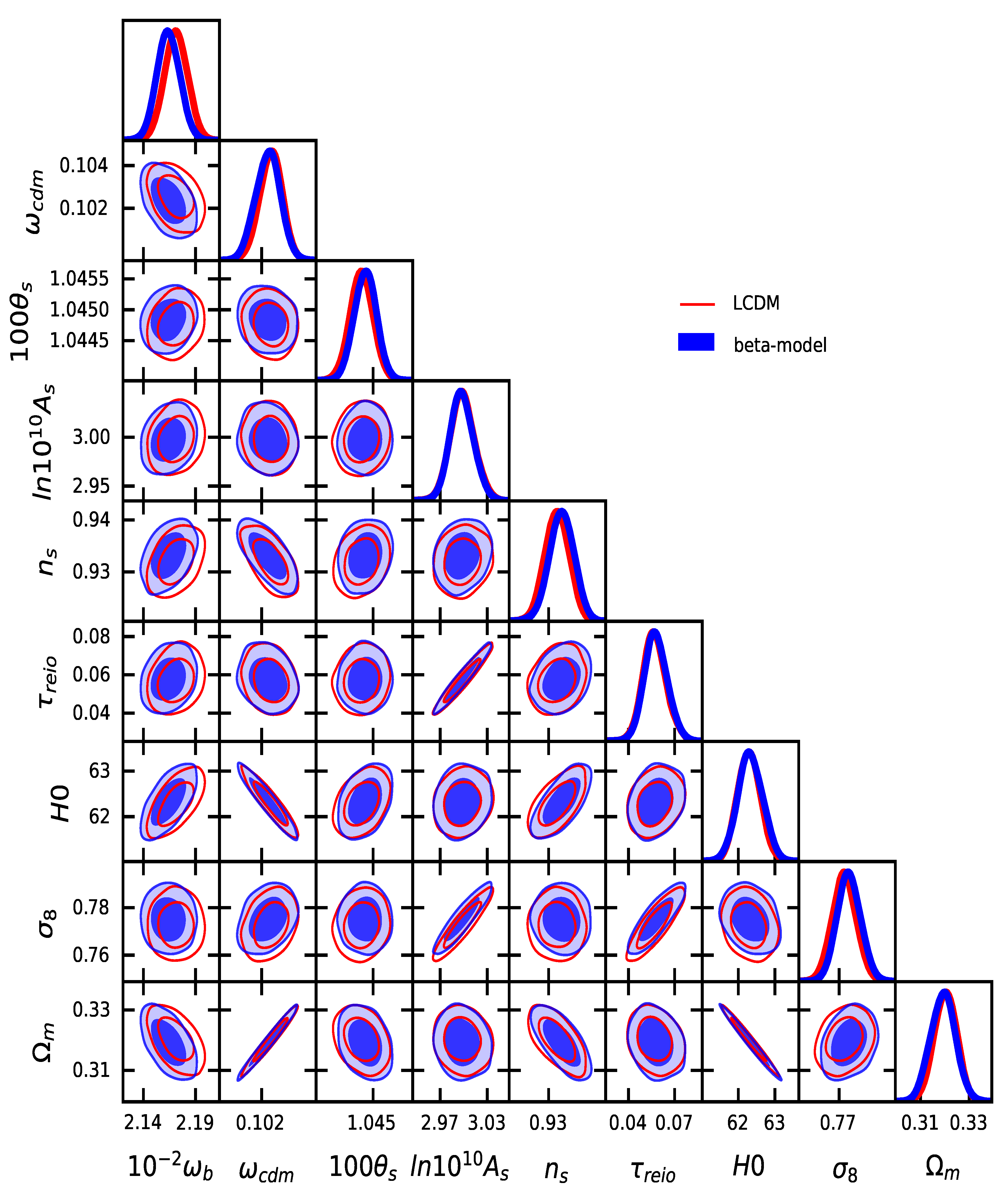
The resulting MCMC chains are analyzed by using GetDist [88] to produce the contour plots. The posterior distributions of the MCMC chains were sampled by means of Metropolis–Hastings algorithm [89,90] in the MontePython runs. The parallel runs were stopped by applying the Gelman–Rubin convergence criterion [91] $R-1\sim 0.02$ and the first 30% of chains were discarded as burn-in. We adopt baseline Gaussian priors, as shown in

Table 1. Flat Gaussian priors on the cosmological parameters used in MCMC numerical analysis.

Parameter	Priors
${\omega }_{\mathrm{b}}{10}^{-2}$	[0.01, 3]
${\omega }_{\mathrm{cdm}}$	[0.01, 0.3]
${\tau }_{\mathrm{reio}}$	[0.01, 0.8]
$n_{\mathrm{s}}$	[0.8, 1.2]
$ln\left({10}^{10}{A}_s\right)$	[1.61, 3.91]
$100{\theta }_{MC}$	[0.5, 10]

: the baryon density is given by ${\omega }_{\mathrm{b}}{10}^{-2}$, ${\omega }_{\mathrm{cdm}}$ represents CDM density, ${\tau }_{\mathrm{reio}}$ is the reonization optical depth, the scalar spectral index is denoted by $n_{\mathrm{s}}$, the amplitude of primordial fluctuations is $ln\left({10}^{10}{A}_s\right)$ and the angular size of the first CMB acoustic peak is represented by $100{\theta }_{MC}$. In the case of $\mathrm{\Lambda }$CDM, the dark fluid parameter is fixed as $w=-1$. Hence, we summarize our results of MCMC analyses in

Table 2. Marginalized constrains on the cosmological parameters (mean values) from GetDist at $68\%$ limits of MCMC chains of each model. The ${\chi }_{tot}^2$ denotes the total mean ${\chi }^2$ of the combined joint datasets.

Parameters	P18+BAO+HST
	$\mathbf{\Lambda }$CDM	$\mathit{\beta }$-Model
${\omega }_b{10}^{-2}$	$2.171\pm 0.011$	$2.{164}_{-0.021}^{+0.022}$
$\omega {}_{cdm}$	$0.10253\pm 0.00067$	$0.1024\pm 0.0014$
$\tau {}_{reio}$	$0.{0571}_{-0.0080}^{+0.0068}$	$0.{058}_{-0.014}^{+0.016}$
$n_s$	$0.9320\pm 0.0029$	$0.{9331}_{-0.0059}^{+0.0056}$
$ln{10}^{10}{A}_s$	$2.{998}_{-0.016}^{+0.015}$	$2.{998}_{-0.029}^{+0.030}$
$100\theta {}_{MC}$	$1.04477\pm 0.00023$	$1.{04484}_{-0.00044}^{+0.00045}$
$H0$	$62.30\pm 0.32$	$62.33\pm 0.66$
${\sigma }_8$	$0.7727\pm 0.0063$	$0.775\pm 0.012$
$S_8$	$0.798\pm 0.0087$	$0.799\pm 0.017$
$\Omega {}_m$	$0.3202\pm 0.0047$	$0.{319}_{-0.0099}^{+0.010}$
w	$-1$	$-0.{7435}_{-0.011}^{+0.016}$
${\chi }_{tot}^2$	$1818.286$	$1814.268$

with the mean marginalized posterior values for the parameters. The resulting contour plots are shown in Figure 1.

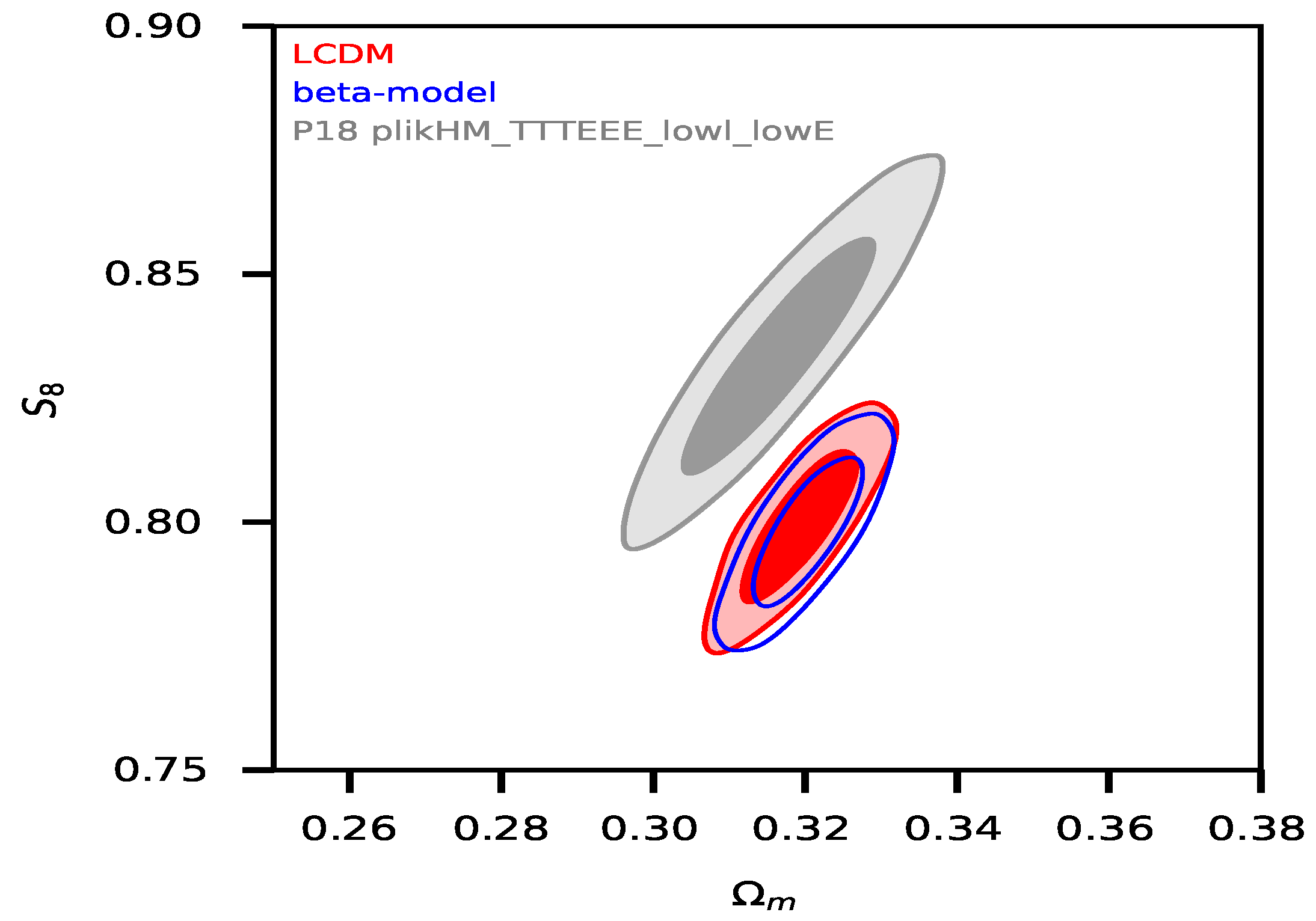
In Figure 2, the plane $(S_8-{\Omega }_m)$ shows the growth amplitude factor $S_8={\sigma }_8{\left({\Omega }_{m0}/0.3\right)}^{0.5}$ that presents lower values $S_8<0.8$ for both models, i.e., $\beta$-model and $\mathrm{\Lambda }$CDM, in contrast with Planck 2018 plik .TTTEEE + low EE + low TT baseline chains. It is important to point out that the values of $\beta$-model for both ${\sigma }_8/S_8$ are lower than the ones of $\mathrm{\Lambda }$CDM within error margins.

In order to check the modification of the value of the gravitational constant during Big Bang nucleosynthesis (BBN) epoch as $z_{\mathrm{BBN}}\sim {10}^9$, we calculate the BBN speed-up factor [92,93]. At the BBN epoch, the bound is about $|\frac{\Delta H^2}{H_{\mathrm{\Lambda }CDM}^2}|<10\%$. From the values of MCMC chains, we obtain the BBN speed-up factor between $\mathrm{\Lambda }$CDM, and the $\beta$-model is roughly 0.2% from the joint datasets P18+BAO+HST, which largely satisfies the bounds on BBN speed-up factor. Concerning the stability of $G_{eff}$, we need to check if it obeys BBN constraints. To do so, we rewrote Equation (47) with its right-shifted parent function as

$$G_{eff}\left(a\right)=\frac{G}{1-9{\gamma }_0{(a-1)}^{1-3w}}.$$

(51)

with ${\gamma }_0$ given by Equation (49). It is worth noting that such a parent function only changes $G_{eff}$ from the growth pattern of the original function in Equation (47) to a decaying behavior. It is worth noting that Equation (51) was implemented in CLASS code by modification of the perturbation module in order to make a correct use of MontePhyton via Python wrapper. The form of Equation (51) attends the constraint $\frac{G_{eff}}{G}{\rfloor }_{a=0}=1$, $\frac{G_{eff}}{G}{\rfloor }_{a=1}=1$, expected for both BBN and solar scales for any $w<0$. We obtain $\frac{G_{eff}}{G}{\rfloor }_{a=0}\sim 0.9995$ and $\frac{G_{eff}}{G}{\rfloor }_{a=1}=1$ , which obeys BBN constraints $|G_{eff}/G-1|\le 0.2$ [94]. Regardless of the value of ${\gamma }_0$, we obtain $\frac{d{G}_{eff}}{da}{/G\rfloor }_{a=1}=0$, which obeys the constraint $\frac{d{G}_{eff}}{da}{/G\rfloor }_{a=1}\simeq 0$ [95]. For early times, BBN constraints are not so stringent [96], and we have $\frac{d{G}_{eff}}{da}{/G\rfloor }_{a=0}>0$.

For the adopted joint data P18+BAO+HST, we find a proximity between the contours in parameter estimation. It calls attention to the fact that we obtain a low value of $H_0$ in both models but they are compatible within error margins for the estimated value of $H_0=65.1_{-5.4}^{+3.0}$ km.s${}^{-1}$. Mpc${}^{-1}$ at 68% C.L. extracted from combining the unreconstructed BOSS DR12 galaxy power spectra, a weak Gaussian prior on the amplitude of the scalar $A_s$ and ${\Omega }_m$ prior from Pantheon supernovae data [97]. Another estimation was made with uncalibrated BAO (6dFGS, MGS and eBOSS DR14 Lyman-$\alpha$ data), obtaining the value of $H_0=65.6_{-5.5}^{+3.4}$ km.s${}^{-1}$. Mpc${}^{-1}$ at 68% C.L. [97]. In terms of tensions, while the $S_8$ tension is solved with $S_8<0.8$, the Hubble tension worsens at$>4.4\sigma$. We find that the adopted dataset prefers a low value of expansion of the Hubble rate, even when compared with the Planck baseline data $H0\sim 68$ km.s${}^{-1}$. Mpc${}^{-1}$. If the analysis is relaxed, we obtain that our result is closer to the one with the recent South Pole Telescope measurements (SPT-3G) [98] combined with WMAP 9-year observations data with $H_0\sim 65.2\pm 7.2$ km.s${}^{-1}$. Mpc${}^{-1}$, as shown in ref. [99], posing a critical scenario. Interestingly, the lower value of Hubble expansion suggests to reveal symptoms of the Planck data anomalies by the combination of the adopted dataset.

Concerning model selection prognosis, we adopt data as Gaussian to perform the Akaike criterion (AIC) [100] classifier to estimate the strength of tension between the data fitting and particular models using maximum likelihood estimation. Thus, for small samples sizes [101,102], we follow the definition

$$AIC={\chi }_{tot}^2+2k\frac{2k(k+1)}{N-k-1},$$

(52)

where ${\chi }_{tot}^2$ is the total mean ${\chi }^2$ of the model, k represents the number of the uncorrelated (free) parameters and N is the number of the data points in a dataset. The difference $|\Delta AIC|=AI{C}_{model\left(2\right)}-AI{C}_{model\left(1\right)}$ represents the Jeffreys’ scale [103] that proposes a classification to the level of statistical tension between two competing models. From Table 2, we have ${\chi }_{tot}^2$ for both models, and we obtain $|\Delta AIC|\sim 2$, which means that in Jeffreys’ scale, the models present a weak tension between them, and they are statistically equivalent. According to Jeffreys’ scale, higher values for the difference $|\Delta AIC|$ indicate more tension between the models.

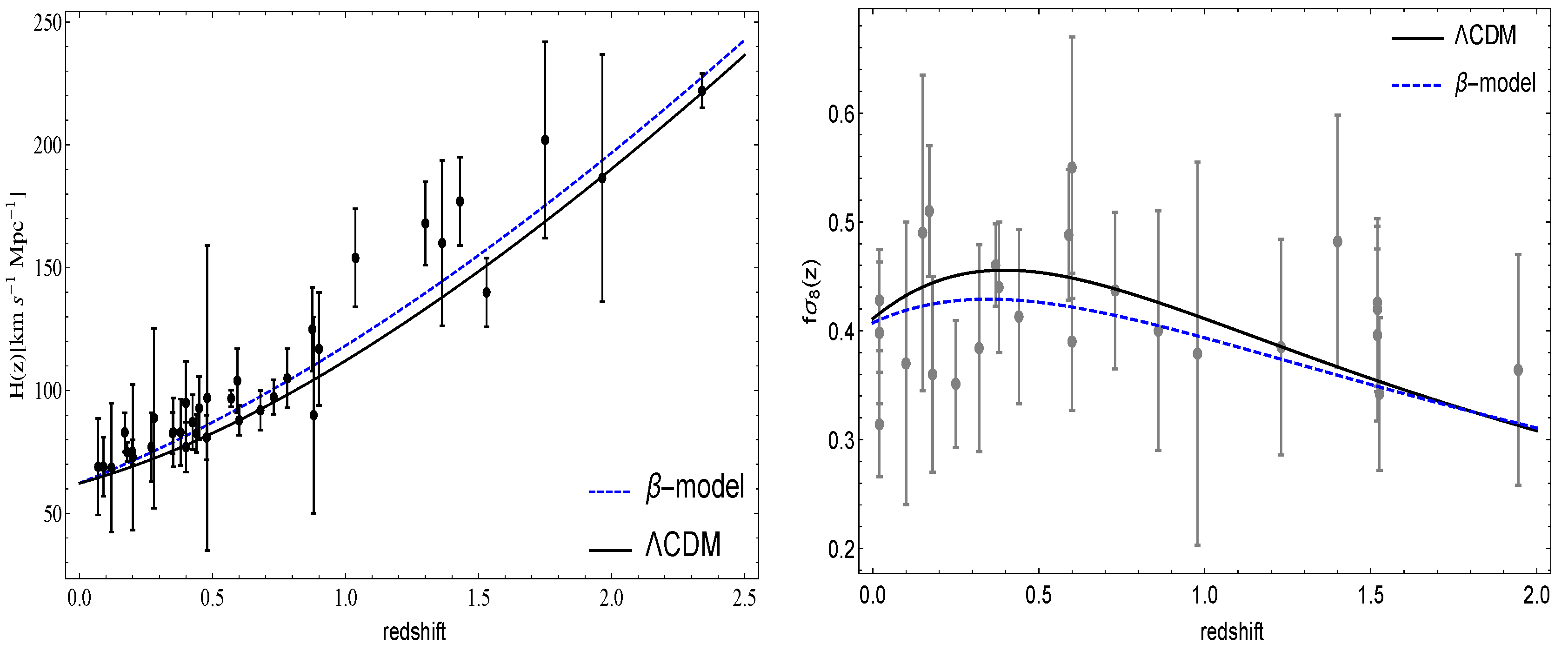
We also check the background evolution of Hubble function $H\left(z\right)$ and the f${\sigma }_8$. The results are presented in Figure 3. For the $H\left(z\right)$ function, we used data points from [75,76] and some “clustering” measurements of $H\left(z\right)$ [77]. The quantity f${\sigma }_8$ allows us a bias-free analysis by defining

$$f{\sigma }_8\left(a\right)\equiv f\left(a\right).{\sigma }_8\left(a\right).$$

(53)

where $f\left(a\right)=\frac{ln\delta }{lna}$ is the growth rate and the growth factor $\delta \left(a\right)$. In the ${\chi }^2$-statistics, one must consider the observed growth parameter $f\left(a_{obs}\right)$ in minimization due to the Alcock–Paczynski effect to take into account redshift-space distortions (RSD). We use the “extended Gold-2018” compilation to the Planck 2018 (TT, TE, EE+lowE) best-fit parameters, as shown in

Table 3. Data points of the “extended Gold-2018” compilation to the Planck 2018 (TT, TE and EE+lowE) best-fit parameters [96] with additional points from BOSS Q [70] and SDSS-IV [71,72,73,74].

Dataset	Redshift	f${\mathit{\sigma }}_8\left(\mathit{z}\right)$	${\mathbf{\Omega }}_{\mathit{m}}$
6dFGS+SnIa	0.02	$0.428\pm 0.0465$	0.3
SnIa+IRAS	0.02	$0.398\pm 0.065$	0.3
2MASS	0.02	$0.314\pm 0.048$	0.266
SDSS-veloc	0.10	$0.370\pm 0.130$	0.3
SDSS-MGS	0.15	$0.490\pm 0.145$	0.31
2dFGRS	0.17	$0.510\pm 0.060$	0.3
GAMMA	0.18	$0.360\pm 0.090$	0.27
GAMMA	0.38	$0.440\pm 0.090$	0.27
SDSS-LRG-200	0.25	$0.3512\pm 0.0583$	0.25
SDSS-LRG-200	0.37	$0.4602\pm 0.0378$	0.25
BOSS-LOWZ	0.32	$0.384\pm 0.095$	0.274
SDSS-CMASS	0.59	$0.488\pm 0.060$	0.30711
WiggleZ	0.44	$0.413\pm 0.080$	0.27
WiggleZ	0.60	$0.390\pm 0.063$	0.27
WiggleZ	0.73	$0.437\pm 0.072$	0.27
Vipers PDR-2	0.60	$0.550\pm 0.120$	0.3
Vipers PDR-2	0.86	$0.400\pm 0.110$	0.3
FastSound	1.40	$0.482\pm 0.116$	0.270
BOSS-Q	1.52	$0.426\pm 0.077$	0.31
SDSS-IV	1.52	$0.420\pm 0.076$	0.26479
SDSS-IV	1.52	$0.396\pm 0.079$	0.31
SDSS-IV	0.978	$0.379\pm 0.176$	0.31
SDSS-IV	1.23	$0.385\pm 0.099$	0.31
SDSS-IV	1.526	$0.342\pm 0.070$	0.31
SDSS-IV	1.944	$0.364\pm 0.106$	0.31

, on the data points of SDSS [57,58,59], 6dFGS [60], IRAS [61,62], 2MASS [61,63], 2dFGRS [64], GAMA [65], BOSS [66], WiggleZ [67], Vipers [68], FastSound [69], BOSS Q [70] and additional points from the 2018 SDSS-IV [71,72,73,74]. These last additional datapoints provide a growth rate at relatively higher redshifts. Moreover, as pointed out in refs. [71,96], to compatibilize the data dependence from the fiducial cosmology and other cosmological surveys, it is necessary to rescale the growth-rate data by the ratio $r\left(z\right)$ of the Hubble parameter $H\left(z\right)$ and the angular distance $D_A\left(z\right)$ by

$$r\left(z\right)=\frac{H\left(z\right)D_A\left(z\right)}{H_f\left(z\right)D_{f}A\left(z\right)},$$

(54)

where the subscript “f” corresponds to a quantity of fiducial cosmology. Similarly, the compatibilization of the related ${\chi }^2$-statistics is also necessary. It can be performed using the expression

$${\chi }^2({\Omega }_{0m},w,{\sigma }_8)=V^i{C}_{ij}^{-1}{V}_j,$$

(55)

where $V^i\equiv f{\sigma }_{8,i}-r\left(z_i\right)f{\sigma }_8(z_i,{\Omega }_{0m},w,{\sigma }_8)$ denotes a set of vectors that go up to $ith$-data points at redshift $z_i$ for each $i=1\cdots N$. N is the total number of data points of a related collection of a data. The set of $f{\sigma }_{8,i}$ data points come from theoretical predictions [96]. The set of $C_{ij}^{-1}$ denotes the inverse covariance matrix. A final important correction concerns the necessity to disentangle the data points related to the WiggleZ dark energy survey which are correlated. Then, the covariant matrix $C_{ij}$ [67] is given by

$$C_{ij}^{wigglez}={10}^{-3}\left[\begin{array}{ccc}6.400& 2.570& 0.000\\ 2.570& 3.969& 2.540\\ 0.000& 2.540& 5.184\end{array}\right]$$

(56)

and the resulting total matrix $C_{ij}^{tot}$

$$C_{ij}^{tot}={10}^{-3}\left[\begin{array}{cccc}{\sigma }_1^2& 0& 0& \cdots \\ 0& C_{ij}^{wigglez}& 0& \cdots \\ 0& 0& \cdots & {\sigma }_N^2\end{array}\right]$$

(57)

where the set of ${\sigma }^2$’s denote the N-variances.

In Figure 3, we have interesting profiles to compare. In the case of evolution of $H\left(z\right)$, the blue dashed curve of $\beta$-model is slightly higher than $\mathrm{\Lambda }$CDM for earlier redshift, but they practically converge for today $z=0$. Then, it is expected that the $f{\sigma }_8$ profile for $\beta$-model should be altered, which is ratified in Figure 3. The $\beta$-model presents a slightly lower $f{\sigma }_8$ at redshift $0.1<z<1$ as compared with the $\mathrm{\Lambda }$CDM profile exactly in the range that the universe speeds up. Our results indicates a slightly more accelerating universe than $\mathrm{\Lambda }$CDM predictions with a fluid parameter $w\sim -0.75$.

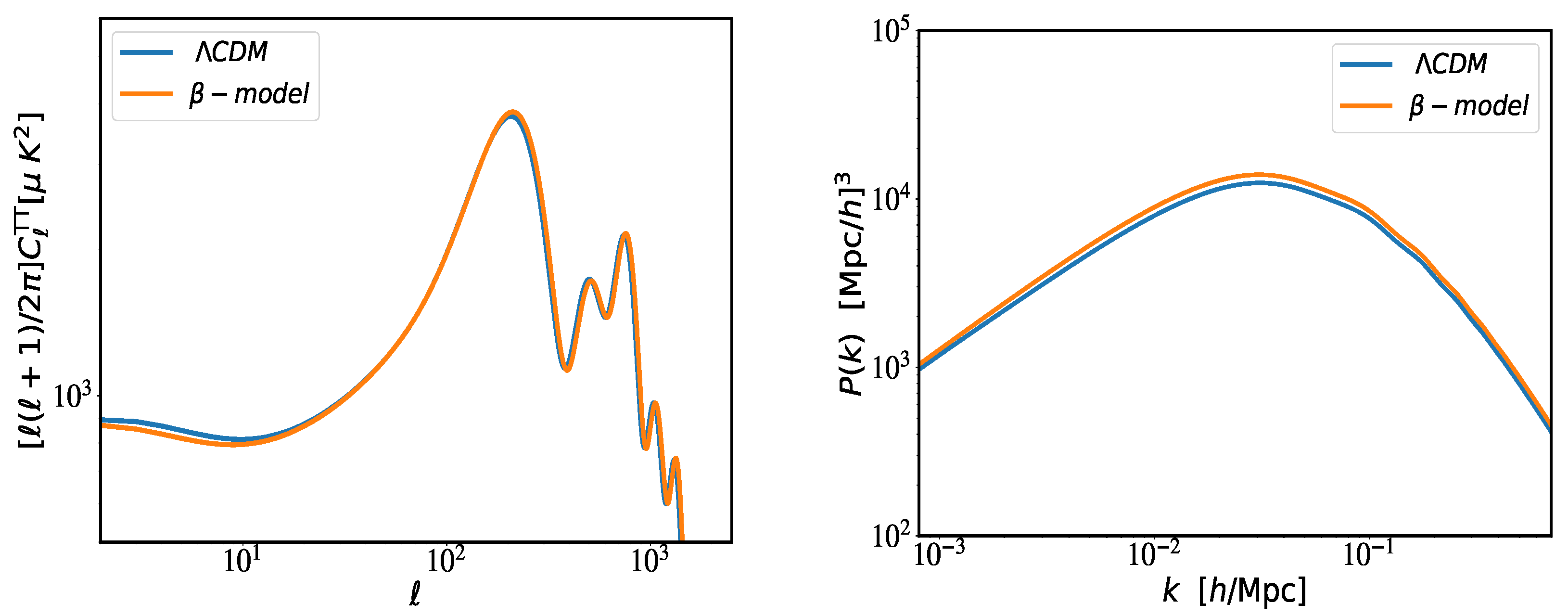
In Figure 4, we obtain in the unlensed CMB TT power spectrum (left panel) and the linear matter power spectrum (right panel) in the pivot scale $k_{*}=0.05$ Mpc${}^{-1}$ with a comparison between the models. As a result, it is shown that the late-time ISW effect is slightly suppressed at lower multipoles in the $\beta$-model (orange line) as compared with flat-based $\mathrm{\Lambda }$CDM (blue line). For higher multipoles, no effective discrepancies are observed in the acoustic peaks and the damping tail, and the unlensed CMB TT power spectrum follows the $\mathrm{\Lambda }CDM$ profile, as expected. It is possible that some slight differences might appear if more BAO data are added from the differences of the SDSS measurements and CMB Planck 2018 probe due to ${\Omega }_m$ and $N_{eff}$ parameters, which will be a topic of further research. In the right panel, the matter power spectrum $P\left(k\right)$ is presented. In contrast with $\mathrm{\Lambda }$CDM results, the central peak is slightly shifted in the $\beta$-model, which suggests being somewhat degenerate with an early DE contribution [104,105].

6. Remarks

From the linear Nash–Greene perturbations of metric, we have shown how to transpose the initial process in the background metric of the embedding of geometries to trigger the geometrical perturbations. The resulting model possesses perturbed field equations hampered by linear Nash’s fluctuations. In a Newtonian gauge, we have obtained $H\left(z\right)$ and the $f{\sigma }_8\left(z\right)$ growth descriptor. Marginalizing the parameters of the model by means of MontePython sampler from joint data P18+BAO+HST, we have obtained the related contours for the $\beta$-model in contrast with the $\mathrm{\Lambda }CDM$ model. We have summarized our results from the numerical analysis in Table 2, In Figure 1, we have presented the triangular plots with contours of the parameters. The analysis on AIC classifiers have led us to $|\Delta AIC|\sim 2$, indicating a statistical equivalence between the models with a weak tension according to Jeffreys’ scale. We have also shown the determination of effective Newtonian constant $G_{eff}$ that matches the Big Bang nucleosynthesis (BBN) constraints, as well as a consistent behavior of Hubble function $H\left(z\right)$ and the $f{\sigma }_8$. Our model also presents a “promising” performance with a suppressed late-time ISW effect at lower multipoles in the $\beta$-model context as compared with $\mathrm{\Lambda }$CDM in the unlensed CMB TT power spectrum. Moreover, a possible degeneracy with an early DE contribution was identified in the matter power spectrum $P\left(k\right)$ and merits further investigation. Concerning tensions on $H_0$ and $S_8/{\sigma }_8$ parameters, we have obtained a curious scenario. For the adopted baseline data on P18+BAO+HST, it prefers a lower expansion rate with $H_0\sim 62.33\pm 0.66$km.s${}^{-1}$. Mpc${}^{-1}$ at 68% C.L. The previous value of $H_0$ for the $\beta$-model is compatible within error margin with ref. [97] by combining the unreconstructed BOSS DR12 galaxy power spectra, with $S_8/{\sigma }_8<0.80$. This suggests that while keeping $S_8/{\sigma }_8<0.8$ solving the tension, higher values on $H_0$ should be obtained with inclusion of more local data, such as Type Ia supernovae (SNe Ia) [75], KiDS [106,107,108,109], DES [110,111] and CFHTLenS [112,113,114]. On the other hand, lower values of expansion of the Hubble rate are compatible with SPT-3G measurements and they seem to reveal the Planck anomalies as the main cause of such issue reinforcing the dilemma of $H0$ tension that might be solved in future CMB data and LSS observations.

References

- Aghanim, N.; Akrami, Y.; Ashdown, M.; Aumont, J.; Baccigalupi, C.; Ballardini, M.; Banday, A.J.; Barreiro, R.B.B.; Bartolo, N.; Basak, S.; et al. Planck 2018 results V. CMB power spectra and likelihoods. A&A 2020, 641, A5. [Google Scholar]
- Sahni, V.; Starobinsky, A. Reconstructing Dark Energy. Int. J. Mod. Phys. 2006, D15, 2105. [Google Scholar] [CrossRef]
- Percival, W.J.; Cole, S.; Eisenstein, D.J.; Nichol, R.C.; Peacock, J.A.; Pope, A.C.; Szalay, A.S. Measuring the Baryon Acoustic Oscillation scale using the Sloan Digital Sky Survey and 2dF Galaxy Redshift Survey. Mon. Not. R. Astron. Soc. 2007, 381, 1053. [Google Scholar] [CrossRef] [Green Version]
- Alam, S.; Ata, M.; Bailey, S.; Beutler, F.; Bizyaev, D.; Blazek, J.A.; Bolton, A.S.; Brownstein, J.R.; Burden, A.; Chuang, C.-H.; et al. The clustering of galaxies in the completed SDSS-III Baryon Oscillation Spectroscopic Survey: Cosmological analysis of the DR12 galaxy sample. Mon. Not. R. Astron. Soc. 2017, 470, 2617. [Google Scholar] [CrossRef] [Green Version]
- Kowalski, M.; Rubin, D.; Aldering, G.; Agostinho, R.J.; Amadon, A.; Amanullah, R.; Balland, C.; Barbary, K.; Blanc, G.; Challis, P.J.; et al. Improved Cosmological Constraints from New, Old, and Combined Supernova Data Sets. Astrophys. J. 2008, 686, 749. [Google Scholar] [CrossRef] [Green Version]
- Jaffe, A.H.; Ade, P.A.R.; Balbi, A.; Bock, J.J.; Bond, J.R.; Borrill, J.; Boscaleri, A.; Coble, K.; Crill, B.P.; de Bernardis, P.; et al. Cosmology from MAXIMA-1, BOOMERANG, and COBE DMR Cosmic Microwave Background Observations. Phys. Rev. Lett. 2001, 86, 3475. [Google Scholar] [CrossRef]
- Izzo, L.; Muccino, M.; Zaninoni, E.; Amati, L.; Valle, M.D. New measurements of Ωm from gamma-ray bursts. Astron. Astrophys. 2015, 582, A115. [Google Scholar] [CrossRef] [Green Version]
- Efstathiou, G.; Lemos, P. Statistical inconsistencies in the KiDS-450 data set. Mon. Not. Roy. Astron. Soc. 2017, 476, 151. [Google Scholar] [CrossRef] [Green Version]
- Allen, S.W.; Rapetti, D.A.; Schmidt, R.W.; Ebeling, H.; Morris, R.G.; Fabian, A.C. Improved constraints on dark energy from Chandra X-ray observations of the largest relaxed galaxy clusters. Mon. Not. R. Astron. Soc. 2008, 383, 879. [Google Scholar] [CrossRef] [Green Version]
- Baxter, E.; Clampitt, J.; Giannantonio, T.; Dodelson, S.; Jain, B. Joint measurement of lensing–galaxy correlations using SPT and DES SV data. Mon. Not. R. Astron. Soc. 2016, 461, 4099. [Google Scholar] [CrossRef] [Green Version]
- Chávez, R.; Plionis, M.; Basilakos, S.; Terlevich, R.; Terlevich, E.; Melnick, J.; Bresolin, F.; González-Morán, A.L. Constraining the dark energy equation of state with H II galaxies. Mon. Not. R. Astron. Soc. 2016, 462, 2431. [Google Scholar] [CrossRef]
- Nemiroff, R.J.; Joshi, R.; Patla, B.R. An exposition on Friedmann cosmology with negative energy densities. J. Cosmol. Astropart. Phys. 2016, 006. [Google Scholar] [CrossRef]
- Santos, B.; Coley, A.A.; Devi, N.C.; Alcaniz, J.S. Testing averaged cosmology with type Ia supernovae and BAO data. J. Cosmol. Astropart. Phys. 2017, 002, 047. [Google Scholar] [CrossRef]
- Kumar, P.; Singh, C.P. New agegraphic dark energy model in Brans-Dicke theory with logarithmic form of scalar field. Astrophys. Space Sci. 2017, 362, 52. [Google Scholar] [CrossRef] [Green Version]
- Velten, H.E.S.; vom Marttens, R.F.; Zimdahl, W. Aspects of the cosmological “coincidence problem”. Eur. Phys. J. C 2014, 74, 3160. [Google Scholar] [CrossRef] [Green Version]
- Sultana, J. The Rh=ct universe and quintessence. Mon. Not. R. Astron. Soc. 2016, 457, 212. [Google Scholar] [CrossRef] [Green Version]
- Sivanandam, N. Is the cosmological coincidence a problem? Phys. Rev. D 2013, 87, 083514. [Google Scholar] [CrossRef] [Green Version]
- Nozari, K.; Behrouz, N.; Rashidi, N. Interaction between Dark Mat-ter and Dark Energy and the Cosmological Coincidence Problem. Adv. High Energy Phys. 2014, 569702. [Google Scholar]
- Maia, M.D.; Monte, E.M. Geometry of brane-worlds. Phys. Lett. A 2002, 297, 9. [Google Scholar] [CrossRef] [Green Version]
- Maia, M.D.; Monte, E.M.; Maia, J.M.F.; Alcaniz, J.S. On the geometry of dark energy. Class. Quantum Grav. 2005, 22, 1623. [Google Scholar] [CrossRef]
- Maia, M.D.; Silva, N.; Fernandes, M.C.B. Brane-world quantum gravity. J. High En. Phys. 2007, 04, 047. [Google Scholar] [CrossRef] [Green Version]
- Arkani-Hamed, N.; Dimopoulos, S.; Dvali, G. The hierarchy problem and new dimensions at a millimeter. Phys. Lett. B 1998, 429, 263. [Google Scholar] [CrossRef]
- Randall, L.; Sundrum, R. Large Mass Hierarchy from a Small Extra Dimension. Phys. Rev. Lett. 1999, 83, 3370. [Google Scholar] [CrossRef] [Green Version]
- Randall, L.; Sundrum, R. An Alternative to Compactification. Phys. Rev. Lett. 1999, 83, 4690. [Google Scholar] [CrossRef] [Green Version]
- Dvali, G.; Gabadadze, G.; Porrati, M. 4D Gravity on a Brane in 5D Minkowski Space. Phys. Lett. B 2000, 485, 208. [Google Scholar] [CrossRef] [Green Version]
- Battyea, R.A.; Carter, B. Generic junction conditions in brane-world scenarios. Phys. Lett. B 2001, 509, 331. [Google Scholar] [CrossRef] [Green Version]
- Heydari-Farda, M.; Sepangi, H.R. Anisotropic brane gravity with a confining potential. Phys. Lett. B 2007, 649, 1. [Google Scholar] [CrossRef] [Green Version]
- Jalalzadeh, S.; Mehrnia, M.; Sepangi, H.R. Classical tests in brane gravity. Class. Quant. Grav. 2009, 26, 155007. [Google Scholar] [CrossRef] [Green Version]
- Maia, M.D. Geometry of the Fundamental Interactions; Springer: New York, NY, USA, 2011; p. 166. [Google Scholar]
- Maia, M.D.; Capistrano, A.J.S.; Alcaniz, J.S.; Monte, E.M. The deformable universe. Gen. Rel. Grav. 2011, 10, 2685. [Google Scholar] [CrossRef] [Green Version]
- Ranjbar, A.; Sepangi, H.R.; Shahidi, S. Asymptotically Lifshitz Brane-World Black Holes. Ann. Phys. 2012, 327, 3170. [Google Scholar] [CrossRef] [Green Version]
- Capistrano, A.J.S.; Cabral, L.A. Geometrical aspects on the dark matter problem. Ann. Phys. 2014, 384, 64. [Google Scholar] [CrossRef] [Green Version]
- Jalalzadeh, S.; Rostami, T. Covariant extrinsic gravity and the geometric origin of dark energy. Int. J. Mod. Phys. D 2015, 24, 1550027. [Google Scholar] [CrossRef]
- Capistrano, A.J.S. Constraints on cosmokinetics of smooth deformations. Mon. Not. Roy. Astron. Soc. 2015, 448, 1232. [Google Scholar] [CrossRef] [Green Version]
- Capistrano, A.J.S.; Cabral, L.A. Evolving extrinsic curvature and the cosmological constant problem. Phys. Scr. 2016, 91, 105001. [Google Scholar] [CrossRef] [Green Version]
- Capistrano, A.J.S.; Cabral, L.A. Implications on the cosmic coincidence by a dynamical extrinsic curvature. Class. Quantum Grav. 2016, 33, 245006. [Google Scholar] [CrossRef] [Green Version]
- Capistrano, A.J.S.; Gutiérrez-Piñeres, A.C.; Ulhoa, S.C.; Amorim, R.G.G. On classical thermal stability of black holes with a dynamical extrinsic curvature. Ann. Phys. 2017, 380, 106. [Google Scholar] [CrossRef] [Green Version]
- Capistrano, A.J.S. Evolution of Density Parameters on a Smooth Embedded Universe. Ann. Phys. 2017, 1700232. [Google Scholar] [CrossRef] [Green Version]
- Capistrano, A.J.S. Lukewarm black holes in the Nash-Greene framework. Phys. Rev. D 2019, 100, 064049-1. [Google Scholar] [CrossRef]
- Capistrano, A.J.S. Linear Nash perturbations with a CMB+Pantheon+H(z) and BAO+DES Y1 joint analysis of cosmic growth expansion. Phys. Rev. D 2021, 103, 043527. [Google Scholar] [CrossRef]
- Capistrano, A.J.S. Sub-horizon modes and growth index in a linear scalar cosmological perturbations. Eur. Phys. J. 2021, 81, 550. [Google Scholar] [CrossRef]
- Capistrano, A.J.S. Fluid approach of linear cosmological Nash-Greene perturbations. Phys. Dark Universe 2021, 33, 100872. [Google Scholar] [CrossRef]
- Capistrano, A.J.S.; Seidel, P.T.Z.; Duarte, H.R. Subhorizon linear Nash-Greene perturbations with constraints on and the deceleration parameter. Phys. Dark Universe 2021, 31, 100760. [Google Scholar] [CrossRef]
- Capistrano, A.J.S.; Cabral, L.A.; Marão, J.A.P.F.; Araújo, C.H.C. Linear Nash-Greene fluctuations on the evolution of S8 and H0 tensions. Eur. Phys. J. C 2022, 82, 1. [Google Scholar] [CrossRef]
- Fan, X.; Bahcall, N.A.; Cen, R. Determining the Amplitude of Mass Fluctuations in the Universe. Astrophy. J. Lett. 1997, 490, 123. [Google Scholar] [CrossRef] [Green Version]
- Brinckmann, T.; Lesgourgues, J. MontePython 3: Boosted MCMC sampler and other features. Phys. Dark Universe 2019, 24, 100260. [Google Scholar] [CrossRef] [Green Version]
- Audren, B.; Lesgourgues, J.; Benabed, K.; Prunet, S. Conservative constraints on early cosmology with MontePython. J. Cosmol. Astropart. Phys. 2013, 1302, 001. [Google Scholar] [CrossRef] [Green Version]
- Audren, B.; Lesgourgues, J.; Benabed, K.; Prunet, S. Monte python: Monte Carlo code for CLASS in Python. Astrophys. Source Code Libr. 2013, ascl-1307. Available online: http://ascl.net/1307.002 (accessed on 30 October 2022).
- Lesgourgues, J. CLASS I: Overview. arXiv 2011, arXiv:1104.2932. [Google Scholar] [CrossRef]
- Blas, D.; Lesgourgues, J.; Tram, T. The Cosmic Linear Anisotropy Solving System (CLASS). Part II: Approximation schemes. J. Cosmol. Astropart. Phys. 2011, 7, 034. [Google Scholar] [CrossRef] [Green Version]
- Dio, E.D.; Montanari, F.; Lesgourgues, J.; Durrer, R. The CLASSgal code for Relativistic Cosmological Large Scale Structure. J. Cosmol. Astropart. Phys. 2013, 11, 044. [Google Scholar] [CrossRef]
- Beutler, F.; Blake, C.; Colless, M.; Jones, D.H.; Staveley-Smith, L.; Campbell, L.; Parker, Q.; Saunders, W.; Watson, F. The 6dF Galaxy Survey: Baryon acoustic oscillations and the local Hubble constant. Mon. Not. R. Astron. Soc. 2011, 416, 3017–3032. [Google Scholar] [CrossRef]
- Anderson, L.; Aubourg, E.; Bailey, S.; Beutler, F.; Bhardwaj, V.; Blanton, M.; Bolton, A.S.; Brinkmann, J.; Brownstein, J.R.; Burden, A.; et al. The clustering of galaxies in the SDSS-III Baryon Oscillation Spectroscopic Survey: Baryon acoustic oscillations in the Data Releases 10 and 11 Galaxy samples. Mon. Not. R. Astron. Soc. 2014, 441, 24–62. [Google Scholar] [CrossRef] [Green Version]
- Ross, A.J.; Samushia, L.; Howlett, C.; Percival, W.J.; Burden, A.; Manera, M. The clustering of the SDSS DR7 main Galaxy sample–I. A 4 per cent distance measure at z = 0.15. Mon. Not. R. Astron. Soc. 2015, 449, 835–847. [Google Scholar] [CrossRef]
- Buen-Abad, M.A.; Schmaltz, M.; Lesgourgues, J.; Brinckmann, T. Interacting dark sector and precision cosmology. J. Cosmol. Astropart. Phys. 2018, 1801, 008. [Google Scholar] [CrossRef] [Green Version]
- Riess, A.G.; Macri, L.M.; Hoffmann, S.L.; Scolnic, D.; Casertano, S.; Filippenko, A.V.; Tucker, B.E.; Reid, M.J.; Jones, D.O.; Silverman, J.M. A 2.4& determination of the local value of Hubble constant. Astrophys. J. 2016, 826, 56. [Google Scholar]
- Samushia, L.; Percival, W.J.; Raccanelli, A. Interpreting large-scale redshift-space distortion measurements. Mon. Not. R. Astron. Soc. 2012, 420, 2102. [Google Scholar] [CrossRef]
- Howlett, C.; Ross, A.J.; Samushia, L.; Percival, W.J.; Manera, M. The clustering of the SDSS main galaxy sample–II. Mock galaxy catalogues and a measurement of the growth of structure from redshift space distortions at z = 0.15. Mon. Not. R. Astron. Soc. 2015, 449, 848. [Google Scholar] [CrossRef] [Green Version]
- Feix, M.; Nusser, A.; Branchini, E. Growth Rate of Cosmological Perturbations at z∼0.1 from a New Observational Test. Phys. Rev. Lett. 2015, 115, 011301. [Google Scholar] [CrossRef] [Green Version]
- Huterer, D.; Shafer, D.; Scolnic, D.; Schmidt, F. Testing ΛCDM at the lowest redshifts with SN Ia and galaxy velocities. J. Cosmol. Astropart. Phys. 2017, 015, 1705. [Google Scholar] [CrossRef]
- Hudson, M.J.; Turnbull, S.J. The growth rate of cosmic structure from peculiar velocities at low and high redshifts. Astrophys. J. Lett. 2013, 751, L30. [Google Scholar] [CrossRef] [Green Version]
- Turnbull, S.J.; Hudson, M.J.; Feldman, H.A.; Hicken, M.; Kirshner, R.P.; Watkins, R. Cosmic flows in the nearby universe from Type Ia supernovae. Mon. Not. R. Astron. Soc. 2012, 420, 447. [Google Scholar] [CrossRef]
- Davis, M.; Nusser, A.; Masters, K.L.; Springob, C.; Huchra, J.; Lemson, G. Local gravity versus local velocity: Solutions for β and non-linear bias. Mon. Not. R. Astron. Soc. 2011, 413, 2906. [Google Scholar] [CrossRef]
- Song, Y.S.; Percival, W.J. Reconstructing the history of structure formation using redshift distortions. J. Cosmol. Astropart. Phys. 2009, 0910, 004. [Google Scholar] [CrossRef]
- Blake, C.; Baldry, I.K.; Bland-Hawthorn, J.; Christodoulou, L.; Colless, M.; Conselice, C.; Driver, S.P.; Hopkins, A.M.; Liske, J.; Loveday, J.; et al. Galaxy And Mass Assembly (GAMA): Improved cosmic growth measurements using multiple tracers of large-scale structure. Mon. Not. R. Astron. Soc. 2013, 436, 3089. [Google Scholar] [CrossRef]
- Sanchez, A.G.; Montesano, F.; Kazin, E.A.; Aubourg, E.; Beutler, F.; Brinkmann, J.; Brownstein, J.R.; Cuesta, A.J.; Dawson, K.S.; Eisensteinet, D.J.; et al. The clustering of galaxies in the SDSS-III Baryon Oscillation Spectroscopic Survey: Cosmological implications of the full shape of the clustering wedges in the data release 10 and 11 galaxy samples. Mon. Not. R. Astron.Soc. 2014, 440, 2692. [Google Scholar] [CrossRef] [Green Version]
- Blake, C.; Brough, S.; Colless, M.; Contreras, C.; Couch, W.; Croom, S.; Croton, D.; Davis, T.M.; Drinkwater, M.J.; Forster, K.; et al. The WiggleZ Dark Energy Survey: Joint measurements of the expansion and growth history at z<1. Mon. Not. R. Astron. Soc. 2012, 425, 405. [Google Scholar]
- Pezzotta, A.; de la Torre, S.; Bel, J.; Granett, B.R.; Guzzo, L.; Peacock, J.A.; Garilli, B.; Scodeggio, M.; Bolzonella, M.; Abbas, U.; et al. The VIMOS Public Extragalactic Redshift Survey (VIPERS): The growth of structure at 0.5<z<1.2 from redshift-space distortions in the clustering of the PDR-2 final sample. Astron. Astrophys. 2017, 604, A33. [Google Scholar]
- Okumura, T.; Hikage, C.; Totani, T.; Tonegawa, M.; Okada, H.; Glazebrook, K.; Blake, C.; Ferreira, P.G.; More, S.; Taruya, A.; et al. The Subaru FMOS galaxy redshift survey (FastSound). IV. New constraint on gravity theory from redshift space distortions at z∼1.4. Publ. Astron. Soc. Jap. 2016, 68, 38. [Google Scholar] [CrossRef] [Green Version]
- Zarrouk, P.; Burtin, E.; Gil-Marín, H.; Ross, A.J.; Tojeiro, R.; Pâris, I.; Dawson, K.S.; Myers, A.D.; Percival, W.J.; Chuang, C.-H.; et al. The clustering of the SDSS-IV extended Baryon Oscillation Spectroscopic Survey DR14 quasar sample: Measurement of the growth rate of structure from the anisotropic correlation function between redshift 0.8 and 2.2. Mon. Not. R. Astron. Soc. 2018, 477, 1639. [Google Scholar] [CrossRef] [Green Version]
- Kazantzidis, L.; Perivolaropoulos, L. Evolution of the fσ8 tension with the Planck 15/ΛCDM determination and implications for modified gravity theories. Phys. Rev. D 2018, 97, 103503. [Google Scholar] [CrossRef] [Green Version]
- Gil-Marín, H.; Guy, J.; Zarrouk, P.; Burtin, E.; Chuang, C.-H.; Percival, W.J.; Ross, A.J.; Tojeiro, R.; Zhao, G.-B.; Wang, Y.; et al. The clustering of the SDSS-IV extended Baryon Oscillation Spectroscopic Survey DR14 quasar sample: Structure growth rate measurement from the anisotropic quasar power spectrum in the redshift range 0.8 < z < 2.2. Mon. Not. R. Astron. Soc. 2018, 477, 1604–1638. [Google Scholar]
- Hou, J.; Sánchez, A.G.; Scoccimarro, R.; Salazar-Albornoz, S.; Burtin, E.; Gil-Marín, H.; Percival, W.J.; Ruggeri, R.; Zarrouk, P.; Zhao, G.-B.; et al. The clustering of the SDSS-IV extended Baryon Oscillation Spectroscopic Survey DR14 quasar sample: Anisotropic clustering analysis in configuration space. Mon. Not. R. Astron. Soc. 2018, 480, 2521–2534. [Google Scholar] [CrossRef] [Green Version]
- Zhao, G.-B.; Wang, Y.; Saito, S.; Gil-Marín, H.; Percival, W.J.; Wang, D.; Chuang, C.-H.; Ruggeri, R.; Mueller, E.-M.; Zhu, F.; et al. The clustering of the SDSS-IV extended Baryon Oscillation Spectroscopic Survey DR14 quasar sample: A tomographic measurement of cosmic structure growth and expansion rate based on optimal redshift weights. Mon. Not. R. Astron. Soc. 2019, 482, 3497–3513. [Google Scholar] [CrossRef] [Green Version]
- Scolnic, D.M.; Jones, D.O.; Rest, A.; Pan, Y.C.; Chornock, R.; Foley, R.J.; Huber, M.E.; Kessler, R.; Narayan, G.; Riess, A.G.; et al. The Complete Light-curve Sample of Spectroscopically Confirmed SNe Ia from Pan-STARRS1 and Cosmological Constraints from the Combined Pantheon Sample. Astrophys. J. 2018, 859, 101. [Google Scholar] [CrossRef]
- Moresco, M.; Cimatti, A.; Jimenez, R.; Pozzetti, L.; Zamorani, G.; Bolzonella, M.; Dunlop, J.; Lamareille, F.; Mignoli, M.; Pearce, H.; et al. Improved constraints on the expansion rate of the Universe up to z∼1.1 from the spectroscopic evolution of cosmic chronometers. J. Cosmol. Astropart. Phys. 2012, 1208, 006. [Google Scholar] [CrossRef] [Green Version]
- Guo, R.; Zhang, X. Constraining dark energy with Hubble parameter measurements: An analysis including future redshift-drift observations. Eur. Phys. J. C 2016, 76, 163. [Google Scholar] [CrossRef] [Green Version]
- Donaldson, S.K. Smooth 4-manifolds with definite intersection form. Contemp. Math. (AMS) 1984, 35, 201. [Google Scholar]
- Taubes, C.H. An introduction to self-dual connections. Contemp. Math. (AMS) 1984, 35, 493. [Google Scholar]
- Lim, C.S. The Higgs particle and higher-dimensional theories. Prog. Theor. Exp. Phys. 2014, 02A101. [Google Scholar] [CrossRef]
- Nash, J. The Imbedding Problem for Riemannian Manifolds. Ann. Math. 1956, 63, 20. [Google Scholar] [CrossRef]
- Greene, R. Isometric Embeddings of Riemannian and Pseudo-Riemannian Manifolds. Memoirs Amer. Math. Soc. 1970, 97. [Google Scholar] [CrossRef]
- Einsenhart, L.P. Non-Riemannian Geometry; Dover: New York, NY, USA, 2005. [Google Scholar]
- Choquet-Bruhat, Y.; York, J.J. Mathematics of Gravitation; Institute of Mathematics, Polish Academy of Sciences: Warsaw, Poland, 1997. [Google Scholar]
- Turner, M.S.; White, M. CDM models with a smooth component. Phys. Rev. D 1987, 56, 4439. [Google Scholar] [CrossRef] [Green Version]
- Zheng, R.; Huang, Q.-G. Growth factor in f(T) gravity. J. Cosmol. Astropart. Phys. 2011, 1103, 002. [Google Scholar] [CrossRef] [Green Version]
- Nesseris, S.; Basilakos, S.; Saridakis, E.N.; Perivolaropoulos, L. Viable f(T) models are practically indistinguishable from ΛCDM. Phys. Rev. D 2013, 88, 103010. [Google Scholar] [CrossRef] [Green Version]
- Lewis, A. GetDist: A Python Package for Analysing Monte Carlo Samples. arXiv 2019, arXiv:1910.13970. [Google Scholar] [CrossRef]
- Lewis, A.; Bridle, S. Cosmological parameters from CMB and other data: A Monte Carlo approach. Phys. Rev. D 2002, 66, 103511. [Google Scholar] [CrossRef] [Green Version]
- Lewis, A. Efficient sampling of fast and slow cosmological parameters. Phys. Rev. D 2013, 87, 103529. [Google Scholar] [CrossRef] [Green Version]
- Gelman, A.; Rubin, D. Inference from Iterative Simulation Using Multiple Sequences. Stat. Sci. 1992, 7, 457. [Google Scholar] [CrossRef]
- Uzan, J.-P. Varying Constants, Gravitation and Cosmology. Living Rev. Rel. 2011, 14, 2. [Google Scholar] [CrossRef]
- Solà, J.; Gómez-Valent, A.; de Cruz Pérez, J. First Evidence of Running Cosmic Vacuum: Challenging the Concordance Model. Astrophys. J. 2017, 836, 43. [Google Scholar] [CrossRef] [Green Version]
- Copi, C.J.; Davis, A.N.; Krauss, L.M. New Nucleosynthesis Constraint on the Variation of G. Phys. Rev. Lett. 2004, 92, 171301. [Google Scholar] [CrossRef] [PubMed]
- Nesseris, S.; Perivolaropoulos, L. Limits of extended quintessence. Phys. Rev. D 2007, 75, 023517. [Google Scholar] [CrossRef] [Green Version]
- Nesseris, S.; Pantazis, G.; Perivolaropoulos, L. Tension and constraints on modified gravity parametrizations of Geff(z) from growth rate and Planck data. Phys. Rev. D 2017, 96, 023542. [Google Scholar] [CrossRef] [Green Version]
- Philcox, O.H.E.; Sherwin, B.D.; Farren, G.S.; Baxter, E.J. Determining the Hubble constant without the sound horizon: Measurements from galaxy surveys. Phys. Rev. D 2021, 103, 023538. [Google Scholar] [CrossRef]
- Dutcher, D.; Balkenhol, L.; Ade, P.A.R.; Ahmed, Z.; Anderes, E.; Anderson, A.J.; Archipley, M.; Avva, J.S.; Aylor, K.; Barry, P.S.; et al. Measurements of the E-mode polarization and temperature-E-mode correlation of the CMB from SPT-3G 2018 data. Phys. Rev. D 2021, 104, 022003. [Google Scholar] [CrossRef]
- Valentino, E.D.; Giarè, W.; Melchiorri, A.; Silk, J. Health checkup test of the standard cosmological model in view of recent cosmic microwave background anisotropies experiments. Phys. Rev. D 2022, 106, 103506. [Google Scholar] [CrossRef]
- Akaike, H. A new look at the statistical model identification. IEEE Transact. Autom. Control 1974, 19, 716. [Google Scholar] [CrossRef]
- Liddle, A.R. Information criteria for astrophysical model selection. Mon. Not. R. Astron. Soc. 2007, 377, L74–L78. [Google Scholar] [CrossRef] [Green Version]
- Sugiura, N. Further analysis of the data by Akaike’s information criterion and the finite corrections. Commun. Stat. A 1978, 7, 13. [Google Scholar] [CrossRef]
- Jeffreys, H. Theory of Probability, 3rd ed.; Oxford University Press: Oxford, UK, 1961. [Google Scholar]
- Das, S.; Souradeep, T. SCoPE: An efficient method of Cosmological Parameter Estimation. J. Cosmol. Astropart. Phys. 2014, 07, 018. [Google Scholar] [CrossRef] [Green Version]
- Hollenstein, L.; Sapone, D.; Crittenden, R.; Schaefer, B.M. Constraints on early dark energy from CMB lensing and weak lensing tomography. J. Cosmol. Astropart. Phys. 2009, 0904, 012. [Google Scholar] [CrossRef] [Green Version]
- Kuijken, K.; Heymans, C.; Hildebrandt, H.; Nakajima, R.; Erben, T.; de Jong, J.T.A.; Viola, M.; Choi, A.; Hoekstra, H.; Miller, L.; et al. Gravitational lensing analysis of the Kilo-Degree Survey. Mon. Not. R. Astron. Soc. 2015, 454, 3500. [Google Scholar] [CrossRef]
- Hildebrandt, H.; Viola, M.; Heymans, C.; Joudaki, S.; Kuijken, K.; Blake, C.; Erben, T.; Joachimi, B.; Klaes, D.; Miller, L.; et al. KiDS-450: Cosmological parameter constraints from tomographic weak gravitational lensing. Mon. Not. R. Astron. Soc. 2017, 465, 1454. [Google Scholar] [CrossRef] [Green Version]
- Conti, I.F.; Herbonnet, R.; Hoekstra, H.; Merten, J.; Miller, L.; Viola, M. Calibration of weak-lensing shear in the Kilo-Degree Survey. Mon. Not. R. Astron. Soc. 2017, 467, 1627. [Google Scholar] [CrossRef]
- Heymans, C.; Tröster, T.; Asgari, M.; Blake, C.; Hildebrandt, H.; Joachimi, B.; Kuijken, K.; Lin, C.-A.; Sánchez, A.J.; van den Busch, J.L.; et al. KiDS-1000 Cosmology: Multi-probe weak gravitational lensing and spectroscopic galaxy clustering constraints. A&A 2021, 646, A140. [Google Scholar]
- Abbott, T.M.C.; Abdalla, F.B.; Alarcon, A.; Aleksić, J.; Allam, S.; Allen, S.; Amara, A.; Annis, J.; Asorey, J.; Avila, S. Dark Energy Survey year 1 results: Cosmological constraints from galaxy clustering and weak lensing. Phys. Rev. D 2018, 98, 043526. [Google Scholar] [CrossRef] [Green Version]
- Troxel, M.A.; MacCrann, N.; Zuntz, J.; Eifler, T.F.; Krause, E.; Dodelson, S.; Gruen, D.; Blazek, J.; Friedrich, O.; Samuroff, S.; et al. Dark Energy Survey Year 1 results: Cosmological constraints from cosmic shear. Phys. Rev. D 2018, 98, 043528. [Google Scholar] [CrossRef] [Green Version]
- Heymans, C.; van Waerbeke, L.; Miller, L.; Erben, T.; Hildebrandt, H.; Hoekstra, H.; Kitching, T.D.; Mellier, Y.; Simon, P.; Bonnett, C.; et al. CFHTLenS: The Canada–France–Hawaii Telescope Lensing Survey. Mon. Not. R. Astron. Soc. 2012, 427, 146. [Google Scholar] [CrossRef] [Green Version]
- Erben, T.; Hildebrandt, H.; Miller, L.; van Waerbeke, L.; Heymans, C.; Hoekstra, H.; Kitching, T.D.; Mellier, Y.; Benjamin, J.; Blake, C.; et al. CFHTLenS: The Canada–France–Hawaii Telescope Lensing Survey–imaging data and catalogue products. Mon. Not. R. Astron. Soc. 2013, 433, 2545. [Google Scholar] [CrossRef] [Green Version]
- Joudaki, S.; Blake, C.; Heymans, C.; Choi, A.; Harnois-Deraps, J.; Hildebrandt, H.; Benjamin, J.; Johnson, A.; Mead, A.; Parkinson, D.; et al. CFHTLenS revisited: Assessing concordance with Planck including astrophysical systematics. Mon. Not. R. Astron. Soc. 2017, 465, 2033. [Google Scholar] [CrossRef]
Figure 1.
The one-dimensional marginalized posterior distributions and two-dimensional contour plots with and C.L. Blue and red colors indicate the -model and CDM, respectively. (For interpretation of the references to color in this figure legend, the reader is referred to the web version of this article.)
Figure 2.
Comparison between the models in the plane () showing contour plots at and C.L. Blue and red colors indicate the -model and CDM, respectively, in contrast, in gray, with Planck 2018 plik.TTTEEE + low EE + low TT baseline chains. (For interpretation of the references to color in this figure legend, the reader is referred to the web version of this article).
Figure 3.
In the left panel, the Hubble function is presented with its evolution in terms of redshift. In the right panel, curves of the evolution show a comparison with the CDM model (black thick dashed). (For interpretation of the references to color in this figure legend, the reader is referred to the web version of this article).
Figure 4.
The left panel shows the unlensed CMB TT power spectrum for the flat CDM (blue line) as compared with the -model (orange line). In the right panel, the matter power spectrum is presented. (For interpretation of the references to color in this figure legend, the reader is referred to the web version of this article).