
Matching with Nonexclusive Contracts †
U.S. Bureau of Economic Analysis, 4600 Silver Hill Road, Suitland, MD 20746, USA
†
The views expressed in this paper are those of the author and do not necessarily represent the U.S. Bureau of Economic Analysis or the U.S. Department of Commerce.
Games 2024, 15(2), 11; https://doi.org/10.3390/g15020011
Submission received: 31 January 2024
/
Revised: 14 March 2024
/
Accepted: 21 March 2024
/
Published: 30 March 2024
(This article belongs to the Special Issue Industrial Organization and Organizational Economics)
Abstract
:A variety of empirical papers document the coexistence of exclusive and nonexclusive contracts within a given market across a multitude of industries. However, the theoretical literature has not been able to generate a differentiable model with the coexistence of these contracts. I rectify the gap in the literature by developing a theoretical model of two-sided matching, in which principals and agents choose between exclusive and nonexclusive contracts with cost-of-effort inefficiencies. I find that the coexistence of contracts relies on cost-sharing between principals, relative bargaining power, and an endogenous outside option. I also find that the pattern of contracts is monotonic with respect to the type distributions of principals and agents.
JEL Classification:
C78; D861. Introduction
There is a large extant literature on exclusive dealing that provides different explanations for contracting parties to prefer nonexclusivity. In some cases, the determining factor is the efficiency of agent effort [1], while in others, firm profitability dictates the contract type [2]. Additionally, the coexistence of different types of contracts in the same market is widely documented in both the empirical and theoretical literature. However, the paucity of theoretical research examining the coexistence of exclusive and nonexclusive contracts is surprising, with [3] representing the only such work, known to this author, to obtain results on contract coexistence.
I remedy this gap in the literature by introducing two-sided heterogeneity into a principal–agent market setting that permits nonexclusive contracting. I seek to address two questions with this set-up:
- Is it possible to obtain contract coexistence in a continuously differentiable setting?
- If contracts can coexist, which productivity types sign which contract, and under what conditions?
In order to answer these questions, I use a very simple principal–agent model with contractible effort, in which an agent can choose to accept a contract from one or two principals. If the agent accepts an exclusive contract, then they cannot work for another principal. When the agent accepts both contracts, the agent incurs an additional cost of effort above the cost required to work for each principal in isolation due to simultaneous effort exertion being more costly. Thus, the trade-off facing the principals is whether to incur this cost and share the wage paid to the agent with another principal, or avoid this cost but pay the entirety of the agent’s wage. This contracting decision is embedded in a market of principals and agents that are heterogeneous in their productivity. Due to the contractibility of effort and risk neutrality of principals and agents, the matching market is one of transferable utility (TU).
I derive the following results. First, I show that it is possible for exclusive and nonexclusive contracts to coexist in a continuously differentiable setting. Second, the matching is positive assortative, even when both types of contracts are signed in a market simultaneously. Third, there are four potential contract patterns, and all are monotonic.1
The first result relies on cost sharing between principals, the endogeneity of the outside option, and effort inefficiencies. These three forces interact to generate a contract switching point in the type distributions of principals and agents. The switching point refers to a principal–agent coalition that is indifferent between either contract type. The coalitions of types lower than this ‘marginal’ coalition prefer one type of contract, while the types above prefer the other contract.
The second result is not guaranteed in a many-to-one matching model, even if the sufficient conditions for a one-to-one matching are satisfied. In a simple TU matching model, the increasing difference condition (ID) must hold in order for the matching to be stable. However, even though my model is one of TU, it is a many-to-one matching model, so when nonexclusive contracts are signed, the Pareto frontier is in as opposed to when under an exclusive contract. Thus, ID is not only insufficient to ensure that a market with coexisting contracts is stable, it is also not necessary. I show that regardless of contract pattern, the stable allocation will always exhibit positive assortative matching (PAM). I discuss the notion of stability that is used in the model in Section 4.
The third result relies on categorizing which principals and agents prefer which contract. This is possible to achieve using the parameter governing the additional cost from simultaneous effort, which I denote by k. The four types of contract patterns that I consider are low types signing exclusive contracts while high types sign nonexclusive contracts, low types signing nonexclusive contracts and high types signing exclusive contracts, all types signing exclusive contracts, and all types signing nonexclusive contracts. Respectively, these are represented by , , , and .
First, consider a matching market in which all coalitions prefer to sign exclusive contracts. In this case, it must be that the effort inefficiencies are large enough to offset the gains from cost sharing for all of the principals and agents in the market (i.e., k is large). If the effort inefficiencies are small enough that the gains from cost sharing outweigh them for all of the principals and agents, then only nonexclusive contracts will be signed in the market (i.e., k is small). The case where contracts coexist in a market occurs for intermediate values of k, which gives rise to the contract patterns and . It is also possible to determine which of the two patterns exhibiting coexistence will be obtained in a market.
The problem faced by the lowest type coalition must be examined in order to determine the contract pattern. If the outside option for the lowest type of agent is unemployment, or a wage of zero, then there is no benefit from cost sharing, because there is no cost for the principals to share. Thus, a nonexclusive contract simply introduces cost inefficiencies, which leads to the lowest principal type choosing an exclusive contract. In this case, the benefit from cost sharing emerges for higher types, since these agents are paid nonzero wages. If the parameter k is small enough, then agents with high enough productivity will command wages that are large enough that principals will be willing to incur the cost of effort inefficiency in order to take advantage of cost-sharing. The result is high types signing nonexclusive contracts and low types signing exclusive contracts. This contract pattern can be seen in the market for actors and actresses. The very best tend to work on multiple projects at the same time, because the studios hiring them can afford to pay for the cost of effort inefficiency. The least capable may only be able to work on a single project at a time, because the studios willing to hire them do not earn enough profit from their projects to offset the cost inefficiency. It is also true that the least capable actors and actresses often face unemployment as their outside option should they fail to find projects on which to work.
Now, suppose the lowest type principal faces unemployment if they fail to sign a contract. This would happen if there are so many principals that even when every agent signs a nonexclusive contract with two principals, there are still some principals that have not signed a contract with an agent. In this case, the agent receives the entirety of the surplus, and the principal receives zero. If k is small enough, then the agent will prefer to receive the surplus from two principals instead of one and will choose to sign a nonexclusive contract. In this example, higher type principals will receive nonzero profits from a match, and thus may not be willing to incur the cost of effort inefficiency. For intermediate values of k, high types will sign exclusive contracts and low types will sign nonexclusive contracts. One industry that exhibits this type of contract pattern is the beer industry. In this case, the most profitable brewers (principals) tend to sign exclusive dealing contracts with a distributor (agent), while less profitable brewers sign nonexclusive dealing contracts.
2. Related Literature and Contribution
In this section, I discuss papers and their results, how they relate to my paper, and the gap that I seek to address with my contribution. First, I provide a short overview of the exclusive contracting literature. Then I examine relevant papers in the matching literature. Additionally, I offer an argument for my contribution and its importance to the literature for each set of papers I consider. I finish by briefly summarizing to reiterate the overall contribution of my paper.
Above all the following papers, the most relevant to the current paper is [3], which examines a many-to-one two-sided matching model of lenders and borrowers in the context of a principal–agent contracting problem. They use the theoretical model to examine the general equilibrium effects of changes in the limited liability constraint due to new bankruptcy laws. While the principal-agent setting is similar, the inefficiency from working for multiple principals arises due to a production function that is concave in the number of principals. Additionally, the heterogeneity in their model is not related to productivity. The lenders are heterogeneous in their fixed cost of monitoring, and borrowers are heterogeneous in their ex ante wealth. Thus, the driving forces in their model operate in almost the exact opposite fashion to this paper, which has productivity heterogeneity and cost inefficiencies. In addition to examining different forces, I provide differentiable sufficient conditions for PAM, which is not a focus of their paper. Therefore, both [3] and this paper contribute to the literature on many-to-one matching in principal-agent markets in very different ways.
2.1. Nonexclusive Contracting
I will separate the nonexclusive contracting literature into two sections: theoretical and empirical. I do this to show that my main contribution is linking the two strands of literature in a way that has not previously been carried out.
Theoretical Literature—Much of the theoretical nonexclusive contracting literature is focused on the effects of exclusivity on the product market and how the product market affects the incentives in the contracting problem. I will not discuss their relation to my model, as I do not explicitly model the product market. Instead, I consider a pair of theoretical papers that extend the nonexclusive contracting setting to account for changes in the outside option [4,5].
The first paper develops a model of loan contracting, in which the outside option is still a fixed amount. However, they show that the results depend on the value of the outside option. Thus, while the outside option is still fixed, they move closer to a true market of principals and agents. In Section 5.1, I show that even this movement toward a market analysis is not sufficient to generate the results I obtain by introducing nonexclusive contracts into a matching market. It is imperative that the market exhibit some type of heterogeneity in order for contracts to coexist. It is also true that even examining the contractual decision in the market setting may not cause both contracts to arise in equilibrium. Matouschek et al. [5] develop a random search model in which buyers and sellers commit to contract breach damages before each buyer realizes their valuation of the good or service being exchanged. The buyers’ valuations act as a source of heterogeneity in their model. Contracts with large enough breach damages are termed exclusive, since neither party contracts with a different buyer or seller ex post. This setup evaluates exclusive contracting in a market with an endogenous outside option. There are multiple important results arising from their model. First, exclusive contracts are more likely when the cost of search is prohibitively high. This should not be too surprising, but it is important nonetheless. Another result is that the market exhibits either exclusive contracts or nonexclusive contracts but not both within the same market. While there is the possibility of contracts coexisting, they find that this particular equilibrium is not stable. The main difference from my model is that the contracts I examine are signed simultaneously, which allows the principals to share the negative externality arising from cost inefficiencies. However, in their model, when a buyer interacts with two sellers, the sellers do not share the cost of the contract break fee. The cost-sharing is absolutely essential to the coexistence of contracts; thus, their model only exhibits a single type of contract in a given market. Additionally, their unstable equilibrium is characterized by all buyer-seller pairs being indifferent between each contract, while my model exhibits only a single principal–agent pair being indifferent between contracts with all others preferring either an exclusive or nonexclusive contract. This indifference for all buyer–seller pairs is due to the breach damages being a choice variable, while it is fixed in my model. My contribution to the theoretical literature on nonexclusive contracting is to develop a model that can generate a market with coexisting contracts similar to those found in the empirical literature.
Empirical Literature—There are a variety of empirical papers that document the existence of exclusive contracts and examine the factors that lead to the adoption of such agreements. Unlike in the theoretical literature, the empirical papers document the existence of exclusive and nonexclusive contracts within the same market. One of the first papers, [1], finds that the efficiency of agent effort leads to higher prevalence of nonexclusive contracts within a market by examining contracts in multiple industries. Sass et al. [2] study exclusive contracting in the property-liability insurance industry and find that the more profitable a firm is within a market, the more likely it is to engage in exclusive contracting. A more recent paper on the U.S. beer market [6] finds that larger markets are more likely to exhibit exclusive dealing since most companies can afford to compensate distributors for foregoing the profits from working for an additional company. My framework offers a theoretical foundation for the observation of exclusive and nonexclusive contracts coexisting within a market that is consistent throughout the empirical literature.
2.2. Two-Sided Matching
There are three subgroups within the matching literature related to the current paper. I discuss these subgroups in turn, as well as the contribution I make to each.
The matching literature includes multiple papers that examine principal–agent models in a two-sided matching framework, (e.g., [7,8,9]. All of these articles focus on the case of one-to-one matching, in which one principal matches with one agent, and the principal offers the agent a single type of incentive contract. These papers are focused on how an endogenous outside option in the contracting problem affects the incentives in the contract. Of course, the authors are also concerned with the conditions for matching to be stable, and whether or not it is assortative. Since I am not interested in the effect of matching on incentive contracts, my principal–agent problem does not involve moral hazard like the papers mentioned above. My main contribution is expanding the principal-agent matching literature to a many-to-one setting by introducing multiple contract types. This makes the endogeneity of the outside option even more important.
The next set of papers also expands the principal–agent matching literature by examining matching markets with multiple types of contracts. In [10], the authors examine the effect of the organizational choice of an enterprise on the price level in a one-to-one matching market. The model involves two sets of suppliers that face a double moral hazard problem and must choose to integrate or not to produce a good. They find that it is possible for both organizational structures to arise in the same market (i.e., some measure of suppliers integrate, while others choose nonintegration). Another related paper [11], considers one-to-one matching by shareholders and managers, where the shareholders can offer managers two different types of contracts, an incentive scheme or a Code of Best Practice (CBP). The incentive contract is the solution to the standard moral hazard problem, while the CBP contract allows the shareholder to specify a given level of effort, but they are still unable to observe the effort of the manager. They find that PAM will only be obtained when one type of contract is signed, while a stable matching with both contracts will be nonassortative. Finally, [12] uses a simple overlapping generations model to examine incentives in long-term versus short-term contracts in a one-to-one matching model. In all of these papers, the authors are able to find conditions that allow both types of contracts to coexist in a stable matching market. My paper extends this strand of the literature to include many-to-one matching with multiple contracts. While these papers consider the effect of incentives on contract choice, I am concerned with the effect the costliness of effort has on contract choice. Thus, rather than examining principals’ use of incentives, I focus on their ability to share the cost of compensating an agent for additional effort.
Before moving on to the related many-to-one matching literature, I acknowledge two papers that provide important results for the stability of many-to-one matching with contracts. Hatfield et al. [13] extend and generalize [14] to accommodate the use of contracts. Then, the work in [15] takes another step in determining the conditions that are sufficient to ensure a stable matching when the gross substitutes condition does not hold. While these papers are concerned with stability conditions rather than providing testable predictions, they are essential to any paper that hopes to do so.
The last group of related papers find differentiable solutions in a many-to-one setting. Azevedo et al. [16] examine hiring decisions when two firms match with many heterogeneous workers prior to competing in a Cournot duopoly. Another paper that uses a differentiable solution is [17]. Their model is similar to [16] in that they consider a firm’s decision to hire many workers; however, they model a market with a continuum of firms and workers. The focus of these papers is on the trade-off a firm faces between hiring more or better workers, rather than a choice between contracts. Additionally, their models have offers being proposed by one to many, whereas the direction of the offers in my model is reversed. My contribution to this nascent literature is to consider many-to-one matching in a principal–agent setting, which allows me to examine the effect of the costliness of effort and the endogeneity of outside options on contract choice.
In summary, I add to the nonexclusive contracting literature by introducing a model that links the theoretical literature to the findings from the empirical literature. My overall contribution to the matching literature is the development of a differentiable many-to-one matching model with multiple types of contracts. I use this model to explore the effects of an endogenous outside option and cost-sharing between principals on contract choice as well as the contract pattern that arises in a matching market. I find conditions that dictate whether the contract pattern involves exclusive contracts for higher productivity types and nonexclusive contracts for lower productivity types, as well as the reverse contract pattern. The first case arises when there are at least twice as many principals as agents in the market, while the latter requires there to be weakly more agents than principals in the market. Within each case, the measure of each type of contract signed in the market depends on the size of the cost inefficiency term.
3. Model
3.1. Matching and Output
I consider a market with risk-neutral principals and agents. The principals are heterogeneous in their assigned type or productivity, which I denote by . Agents are heterogeneous in their assigned type or productivity, which I denote by . The type spaces and are subintervals of . The CDF for principal productivity is with a PDF, . The CDF for agent productivity is with a PDF, . Additionally, I assume that the measure of principals and agents are and , respectively, so that the ratio of principals to agents is . In the main text, I focus on the cases where and . These represent cases in which one side of the market is guaranteed a match partner regardless of the equilibrium contract pattern. When this is not the case, additional assumptions must be made in order to pin down an equilibrium matching pattern, which distracts from the main focus of the paper. I leave a general analysis of the matching functions as well as intermediate values of for the extension section of the Appendix C. In this market, a principal can be viewed as the owner of a project, while an agent is a manager. Each agent is capable of managing two projects, however, a principal only needs a single agent to manage a project. For simplicity, I assume it is prohibitively costly for an agent to manage more than two projects at a time. Endogenizing the number of projects an agent can manage adds additional complications without affecting the main results of this paper in a meaningful way.
Next, I examine the output generated by an arbitrary principal–agent pair, which I denote .2 The output for a principal–agent pair is represented by the production function , where , and is the effort exerted by the agent on the project for principal . The agent incurs the following cost of effort:
where designates an exclusive or nonexclusive contract, respectively. The cost inefficiency from working for two principals simultaneously is represented by and is equal to zero when the agent works for only one principal. The inefficiency stemming from an agent working for more than one principal is a standard assumption in the literature on multiprincipal contract theory. It can be a direct effect via concavity of the production function in the number of principals per agent as in [3], or it can be an indirect effect through the cost of effort function seen in [18] and in the context of multiple tasks in [19,20]. Since the cost function only contains the effort exerted on a single principal’s project, the optimal choice of effort in a nonexclusive contract for principal is not affected by the effort choice for principal . Thus, while the extensive and intensive margins of the output are affected by the agent’s decision to work for another principal, neither are affected by how much the agent works for the other principal.3 Imagine a consulting firm currently contracted with a single client that operates in the manufacturing industry. Suppose the consulting firm accepts an additional contract with another client that operates in the tech industry. It receives compensation from each client, but the clients are not required to compensate the consulting firm for time spent on the other client’s project. In order to handle the increased workload, the consulting firm divides its employees into two teams with each focusing on a single client. As a result, the effort for each team becomes more costly; however, the effort exerted by one team does not impact the effort exerted by the other team.
Finally, consider the definition of matching that is given below:
Definition 1
(Matching, [21]). A matching, , is a mapping from onto s.t. and :
- (i)
- and if .
- (ii)
- , , and if .
- (iii)
- iff .
In words, (i) states that the number of elements in a principal’s matching set, , is equal to one, and if the principal remains unmatched, then it matches with itself; (ii) the matching includes all principals and the agent, the agent cannot match with more than two principals, and if the agent remains unmatched, then it is matched to itself; (iii) a principal is matched to an agent if and only if that agent is also mapped to that principal. This definition allows for unemployment on either side of the market, one-to-one matching, and two-to-one matching between two principals and one agent.
3.2. Contracts and Timing
First, I introduce the definition of contracts that I use in my model. I perform this by considering the principal-agent pair, .4 I assume that the principals hold the bargaining power and make take-it-or-leave-it offers to the agents. Unlike the principal–agent matching models mentioned in Section 2.2, effort is observable in my model, so the principals do not use incentive contracts. Instead, the principals choose the effort level that maximizes the output minus the cost of effort, for which the principal must compensate the agent in order to ensure the agent receives utility equal to their outside option. This is the simplest setting in which it is possible to examine the impact of cost-sharing, relative bargaining power, and an endogenous outside option on the prevailing contract pattern in a market. Since the effects of incentives are not the main focus and complicate the analysis, a model with moral hazard is left for future research.5
For the principal–agent pair, , I denote the optimal effort by . The other portion of a contract specifies the wage that the principal will pay the agent upon the realization of the output for the pair. The wage offered by principal is , which differs depending on whether the contract is exclusive or nonexclusive. Thus, the entire contract offer by the principal specifies an optimal effort level and wage, and it is denoted by .
Now, I turn to the timing of events. The model proceeds in three stages. In Stage 1, a single agent matches with one or two principals. In Stage 2, the principals make contract offers . In Stage 3, the agent exerts the agreed-upon effort, the output is realized, and the payments are made. The sequential nature of the model makes it possible to solve through backward induction.
3.3. Principal–Agent Pair
In this section, I examine the contracting problem for the principal–agent pair, . For each type of contract, the principal needs to maximize the output generated by the pair by choosing the effort the agent must exert, while also ensuring the agent receives at least the utility from their outside option. This problem is written as follows:
Here, the profit for a given contract type, d, going to the principal is denoted by , while the utility the agent receives is . The outside options for the principal and agent are and , respectively, and is the cost of effort function for a contract of type d with principal . The problem is solved by plugging the agent’s individual rationality constraint, (3), into (2), which gives the following:
where . Recall that the optimal contract in this setting entails the principal choosing the effort level that will maximize the output minus the cost of effort. Since the outside option is not a function of the agent’s effort, maximizing (5) with respect to results in the same optimal effort level.
The first-order condition for the problem is , where the subscripts represent derivatives. The FOC can be solved for the optimal effort level, , where if the contract is exclusive. The optimal effort level can be plugged into the RHS of (5) to obtain the maximized principal profit, , which I denote by
where
Throughout the remainder of the paper, I refer to as the surplus generated by a matched pair. As an aside before discussing the feasibility of contracts, it is important to consider the impact of effort inefficiencies in terms more applicable to real-world situations. Given the two potential surpluses in (7), we can calculate the percent change in surplus that an agent generates for an individual principal when switching from an exclusive to a nonexclusive contract as follows:
For example, if 0, the percent change is . Since , the percent decrease is between 0 and 50 percent.
Definition 2
(Feasibility). A contract, , is feasible for the principal–agent pair, , if it satisfies the IR constraints for the principal and agent, and the choice of effort maximizes the output generated by the principal–agent pair.
Note that the maximized principal profit in (6) is the bargaining frontier for the principal–agent pair.6 Since the utility of the agent enters the bargaining frontier linearly, the matching market will be one of transferable utility. This means the wage in a given contract is used to ensure that (3) is satisfied. Thus, all the contracts considered in the model are feasible.
4. Equilibrium Matching and Stability
I separate this section into three parts. Section 4.1 considers the matching between principals and agents, the notion of PAM, and introduces some notation for the equilibrium definition. In Section 4.2, I discuss the notion of stability that is used as the solution concept in the model. I conclude by introducing the equilibrium definition in Section 4.3.
4.1. Principal–Agent Matching
In this stage, I examine the equilibrium matching and discuss the sorting pattern in the principal–agent market. In order to maximize their payoff from a match, each principal must optimally choose an agent
The function is the combined bargaining frontier for principal–agent pair , when the agent receives utility from principal i, and the cost inefficiency term is k. The solution to (9) is given by the equilibrium matching. Recall, from Definition 1, a matching is a mapping from the union of the type spaces onto itself. I use two separate functions to distinguish when the mapping is one-to-one and when it is two-to-one. I write the matching as , where represents the matching in an exclusive contract, and represents the matching in a nonexclusive contract offered by principal i.
In order to give a clearer picture of the problem, I examine the bargaining frontier for each contract separately. The necessary and sufficient condition for PAM is that the surplus function satisfies ID. In the current context, for a given contract, the condition is as follows:
for any and . This requires principal to have a higher willingness to pay than principal for agent . The differentiable version of this condition is that the cross-partial of principal and agent types is weakly positive, , which is known as type–type complementarity. It is easy to see, from the functional form used in the model, that the differentiable version of (10) is satisfied for each type of contract in isolation.
Now, I consider the problem facing a given principal when choosing an agent. Remember from Section 3.3 that the utility an agent receives can be replaced by the wage offered by a principal. Thus, a principal must solve the following problem to maximize their payoff from a match:
Here, I write the bargaining frontier as a function of the principal and agent types while suppressing the utility and cost inefficiency term for exposition. The FOC for (11) is
where subscripts are used to denote partial derivatives. Plugging in the equilibrium matching function for each contract type gives the following ODEs for the utility functions:
The solutions to (13) give the equilibrium utility functions for each contract, and .7 However, this is only part of the solution for an equilibrium matching, since it does not involve comparing the payoffs from one contract to the other. The conditions for a nonexclusive contract to be preferred by the principal-agent pair are
where I suppress the arguments for exposition, and represents the total utility the agent receives in a nonexclusive contract.8 The inequalities in (14) simply require the principal and agent to receive higher payoffs under a nonexclusive contract than an exclusive contract. If the contracts coexist in a market, then it must be that the inequalities in (14) hold with equality for at least one principal-agent pair, which I call the marginal coalition. I write this principal–agent pair as , where . I define the marginal coalition here so that I may introduce the concept of a matching market outcome before proceeding to the sections on stability and market equilibrium. I discuss the marginal coalition in more detail in Section 5, when I examine the contract patterns.
Let be the assignment object that contains all the relevant information about the principal-agent assignment game. The other equilibrium object is the menu of contracts, .
Definition 3
(Matching Market Outcome). An outcome for a market is the tuple .
Definition 4
(Constrained Pareto Optimal). A contract for a principal–agent pair is Constrained Pareto Optimal if there is no other feasible contract for which both principal and agent can be made better off.
Note that the two definitions above say nothing about stability.9 However, it will become clear that a stable equilibrium assignment will be a matching market outcome with Constrained Pareto Optimal contracts.
4.2. Stability
Unlike the one-to-one case, in a many-to-one matching model, the equilibrium assignment must be robust to deviations by coalitions. In the current setting, this would involve a group of principals and an agent deviating to match with each other. However, it has been shown by [22] that robustness to deviations by pairs is sufficient to ensure a stable matching as long as preferences are responsive.10 Thus, the standard solution concept in many-to-one matching models is pairwise stability. If preferences are not responsive, it is not even guaranteed that a stable matching exists. Since the maximum number of principals that can be assigned to a given agent is two, group stability is implied by pairwise stability in my setting even without responsive preferences. Thus, I use the following definition:
Definition 5
(Pairwise Stability). A matching is pairwise stable if it satisfies individual rationality and the no blocking condition:
- 1.
- Individual Rationality:
- (i)
- Principals: .
- (ii)
- Agents: and .
- 2.
- No Blocking: If
- (i)
- Then .
- (ii)
- And if , then .
The individual rationality condition states that principals prefer remaining matched to unmatched, and agents cannot match with more principals than their quota, , and prefer all principals in their matching to removing one of the principals. The no-blocking condition requires that if a principal p prefers another agent a to the one with which p is matched, then a prefers the matching to replacing a principal in that matching with p, and if the agent has not met their quota, then the agent prefers the current matching to adding p. This definition is quite general, as it can apply to a case where a large number of principals match with a given agent.11 Additionally, the definition makes no statement about whether the matching will involve monotonic or nonmonotonic contract patterns.
4.3. Decentralized Principal–Agent Market
In this section, I introduce the definition of equilibrium for the model.
Definition 6
(Constrained Pareto Optimal Market Equilibrium, CPOME). A tuple is a CPOME if:
- 1.
- The menu of contracts is feasible and Constrained Pareto Optimal.
- 2.
- The assignment object is pairwise stable.
I denote a CPOME as , where I use the stars to indicate that the matching market outcome is a stable equilibrium. Again, the definition above makes no assumption about the contract pattern arising in a CPOME. I examine the conditions for the stability of certain contract patterns in more detail in the following section.
5. Analysis
This section is designed to explore the variety of results in the model. In Section 5.1, I discuss the effect of embedding the principal-agent problem within the matching market. Then, I categorize the potential contract patterns and the conditions for these patterns to be obtained in Section 5.2. Section 5.3 examines the utility functions that obtain for different measures of principals and agents, as well as how these functions are affected by changes in k.
5.1. Isolation vs. Market
In this section, I explore the differences between an isolated principal–agent problem and the principal–agent market. The distinction is particularly important in the principal–agent literature, because two-sided matching endogenizes the outside options for both parties. In the following analysis, I consider two cases. The first case is when there are at least as many agents as principals (), and the second is when there are twice as many principals as agents (). In order to conduct the analysis, I shut down the endogeneity of the outside option for the principals and agents. However, I still allow for heterogeneity in principal and agent types. To be clear, there is no interaction between principals and agents of different types, so it could be viewed as a continuum of isolated markets. The reason for this approach is that a continuum of separate markets can be easily compared with the endogenous matching model. What is of particular interest is how the contract patterns and marginal coalitions are affected by removing the endogenous outside option. I suppress arguments throughout the analysis for exposition.
- Case 1:
Here, one can think of each market as having two principals and two agents. In this setting, the outside options when a principal or agent does not sign any contract are and , respectively. I use the superscripts i and j to designate the different principals and agents. Since the outside options are exogenous, they are not affected by the productivities of a given market. Each of the agent’s individual rationality constraints will be binding, because one agent would be left out if a nonexclusive contract were signed. Consequently, the comparison of each principal’s utility across contracts determines the contract that is chosen. Thus, for a given principal, we have the following comparison:
I use this condition in the subsequent analysis for .
Recall that this setting involves a continuum of isolated markets, which I assume to have productivities in the type spaces and . Thus, I have the least productive market with types and . I further separate the analysis into two subcases, in which the least productive market signs exclusive contracts and nonexclusive contracts.
First, I consider the subcase in which the principals and agents from the least productive market choose to sign exclusive contracts. In order for the least productive market to prefer exclusive contracts
In order to see which contracts more productive types prefer, I simply need to differentiate (16) with respect to a, which gives the following:
The inequality in (17) is positive, due to the cost inefficiency term in and because the outside option is not a function of agent type (i.e., ). Thus, all the isolated markets prefer to sign exclusive contracts. From (17), one can see that the only way to flip the inequality is for the outside option of the agent to be endogenous.
Now, I consider the subcase in which the least productive market exhibits nonexclusive contracts. The principals and agents from this market will prefer nonexclusive contracts when the following inequality holds:
Like in the previous subcase, the contract preference for more productive types can be determined by differentiating (18) with respect to a to obtain the following:
Now, the cost inefficiency term leads to the inequality in (19) being negative. The implication is that a market with a high enough level of productivity will prefer exclusive contracts. Again, the only way to counteract this movement toward exclusive contracts is for the outside option to be endogenous.
Result 1.
When , the following hold:
- 1.
- If the lowest type of market exhibits exclusive contracts, then all other markets will also exhibit exclusive contracts.
- 2.
- If the lowest type of market exhibits nonexclusive contracts, then markets with high enough productivity will sign exclusive contracts.
It should be clear after the analysis above that an endogenous outside option can change Result 1. Thus, the matching model could generate different results. Note that the inefficiency term acts as a wedge in the nonexclusive surplus function, so that the absolute difference between the exclusive and nonexclusive surplus functions grows as the productivity types increase. Thus, if (16) is satisfied for a given market, then it will be satisfied for all higher productivity markets since the outside option is fixed.
- Case 2:
In this section, I determine if the results from the previous case are reliant on the relative measure of principals to agents, or if they are more general. In the isolated market setting, this case would involve two principals and one agent per market. Now, each principal’s individual rationality constraints are binding, because one will be left out if the agent accepts an exclusive contract. As a result, the contract choice relies entirely upon each agent’s preference across contracts, which is given by
where the equivalence is due to the principals being the same productivity type within a given market.
Similar to the case where , I separate the analysis into a subcase for when the least productive market signs each contract type. First, consider when the least productive market prefers exclusive contracts.
Since principals are of the same type, we can simplify (21) and differentiate with respect to a to obtain the following:
The outside option is fixed, so the derivative of with respect to a is zero. Since is an assumption in the model, (22) is negative, which implies lower productivity markets will sign exclusive contracts and higher productivity markets will sign nonexclusive contracts. The only force that could prevent the switch is an endogenous outside option for a principal.
In the other subcase, where nonexclusive contracts are signed in the least productive market, the inequality in (21) becomes the following:
Now, there is no switch to exclusive contracts, so all markets exhibit principals and agents signing nonexclusive contracts. Again, an endogenous outside option for the principal could cause (24) to be negative, which would lead to higher productivity markets signing exclusive contracts.
Result 2.
When , the following hold:
- 1.
- If the lowest type of market exhibits exclusive contracts, then markets with high enough productivity will sign nonexclusive contracts.
- 2.
- If the lowest type of market exhibits nonexclusive contracts, then all markets will sign nonexclusive contracts.
From the preceding analysis, it is evident that two of the main components driving the contract patterns are cost sharing between principals in the presence of effort inefficiencies, and the absence of an endogenous outside option. A third force is the bargaining power between principals and agents. When one side of the market has all of the bargaining power, the individual rationality constraint for the opposite side is binding. This is why the contract switch is reversed in Cases 1 and 2, even without an endogenous outside option. In Section 5.2, I show how the results change when the outside option is endogenized.
5.2. Equilibrium Contract Patterns
First, I show how I derive the contract pattern. Then, I introduce propositions that dictate the pattern of contracts in a market and the conditions for these contract patterns to be stable. I also discuss how each of these cases compares to the corresponding fixed outside option example derived in Section 5.1. Recall the terms for each contract pattern: , , , and . These represent exclusive throughout, nonexclusive throughout, exclusive at the top, and nonexclusive at the top of the market, respectively.
5.2.1. Threshold Function
Before examining each potential contract pattern, I discuss the method by which the contract pattern can be derived. Note that the contract choice depends on the individual rationality constraints of the principals and agents. Recall from (14) that a nonexclusive contract is preferred by principals and agents if
The agent in the marginal coalition will be indifferent between contract types so that, . Plugging this into the individual rationality constraint for the principal in (25), and rearranging gives The agent in the marginal coalition will be indifferent between contract types so that, . Plugging this into the individual rationality constraint for the principal in (25), and rearranging gives
where (26) stands for Local Nondeviation Condition. It is called the (26), because it considers local deviations across contracts, where local refers to the principal and agent types. If there is a contract switching point in the market, the (26) will hold with equality for some marginal coalition, , where . Rewriting (26) for the marginal coalition gives
where I include the arguments of the functions and represent the entire surplus from a nonexclusive contract by .12 Note that due to the functional form, (27) can be solved for k and evaluated at a proposed assignment to obtain
where is the quasi-inverse of , and (28) stands for threshold function. The threshold function gives the value of k that will induce a contract switching point at a given marginal agent of type in the proposed equilibrium assignment object . I use this threshold function in subsequent sections to determine which contract patterns arise in equilibrium.13
5.2.2. More Agents than Principals
When there are more agents than principals, the outside option of the lowest productivity agent in the market is zero, because if an agent fails to sign a contract they will be left out of the market or, in other words, unemployed. Consequently, the lowest type principal will receive the total surplus under either contract, which will always be more under an exclusive contract, since . We can then use the inequality in (15) but replace the terms with their matching market counterparts. For every agent type, the comparison is between contracts with the same principal type, which is represented by in both the exclusive and nonexclusive surplus functions.14 Thus, the nonexclusive contract will be preferred if
Differentiating both sides of the inequality with respect to a and suppressing arguments for exposition gives the following:
Using the exclusive contract ODE in (13) to replace and substituting in the functional forms gives
Rearranging and canceling obtain the following condition on k:
where arguments are suppressed for exposition. The condition in (32) shows that there are values of for which nonexclusive contracts will be preferred if the distribution is defined over a sufficiently long interval. Thus, we arrive at the following proposition.
Proposition 1.
If , then the potential contract patterns are and .
Proof.
See Appendix A.2. □
Recall from Result 1 in Section 5.1 that either all of the isolated markets would sign exclusive contracts, or less productive markets would sign nonexclusive contracts and more productive markets would sign exclusive contracts. Thus, the main difference is in the direction of the contract switch. There are two reasons behind this reversal. The first is the endogeneity of the outside option, which I indicated as important in Section 5.1. In the matching market, this leads to a switch from exclusive contracts to nonexclusive contracts when moving up the type distribution. The second factor is related to the contracts signed by the lowest productivity pair. In the isolated markets example, nonexclusive contracts will be signed in the least productive market only if the outside option for the agent is nonzero, which can be seen in (18). However, as previously mentioned, when , the outside option for the lowest productivity agent in the matching market is zero, because if an agent fails to sign a contract, they will be left out of the market. If the outside option in the isolated case is restricted to zero, then the central result from introducing the principal–agent problem into a matching market is that there is a contract switching point in the market.
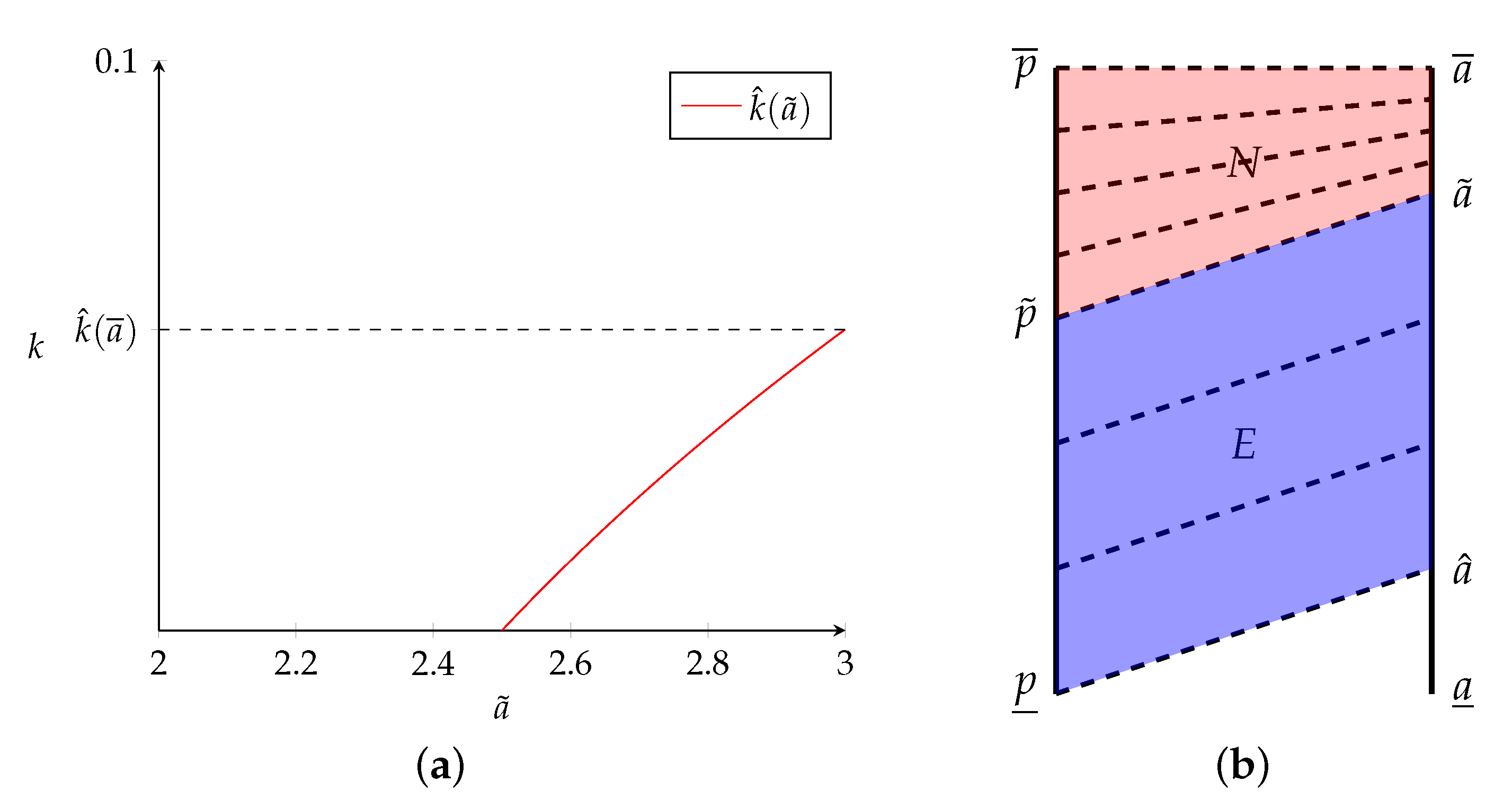
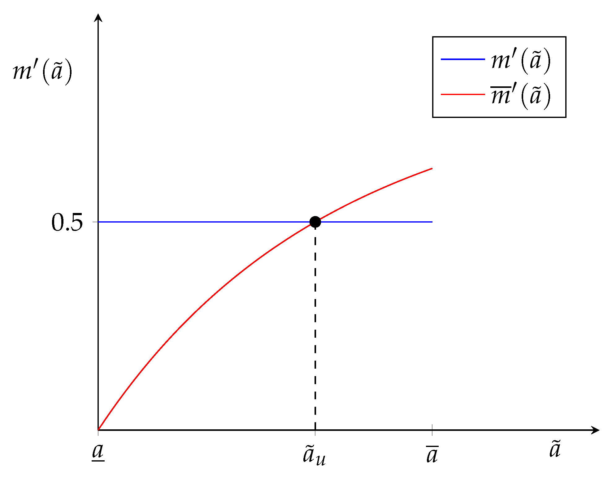
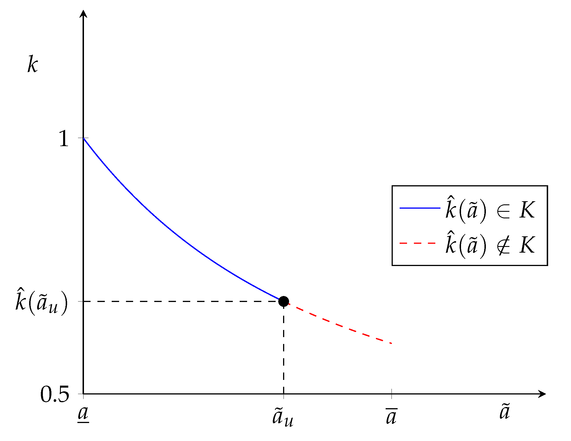
Now, I discuss when it is possible for a contract switch to occur in a matching market using a simple example. Consider the threshold function in Panel (a) of Figure 1 below for principal and agent productivity types distributed uniformly over with and . Notice that nonexclusive contracts will only obtain if , and remember that . In Panel (a) of Figure 1, 0, which can be translated to percent change as .15 Thus, the contracts will coexist in this setting only if the cost inefficiencies are relatively small.
Panel (b) of Figure 1 is an example of the contract pattern that will be obtained under Proposition 1 when cost inefficiencies are small enough to induce a contract switch. In this figure, the pink region indicates the coalitions entering nonexclusive contracts, and the blue region indicates the coalitions entering exclusive contracts. Note the measure of agents at the bottom of the distribution that remain unmatched. I denote the lowest type of agent in the market by , so that agents with types are unemployed under the equilibrium assignment. Panel (b) of Figure 1 represents a case in which the type distributions have the same length of supports. Since , the implication is that the density of agents within the support is weakly larger than the density of principals.
In the present case, k can be viewed as a per-unit usage cost for a technology that manages accounts for multiple principals. Thus, as the technology becomes more costly (an increase in k) fewer agents are productive enough to offset the extra cost. For a given market, it may be that the technology is too costly, so that no agents are observed working for more than one principal.
Below, I provide a proposition for the stability of the contract pattern in this setting.
Proposition 2.
If , then the stable matching is or .
Proof.
See Appendix A.3. □
Corollary 1.
there is no stable matching pattern when .
Proposition 2 states that there is a single interval of values of k, denoted by K, for which a market will exhibit or as a contract pattern. Corollary 1 indicates that when k is larger than the supremum of K, the LNDC is not robust to global deviations, thus, the contract pattern is not stable.
5.2.3. More Principals than Agents
When there are at least twice as many principals as agents, the outside option of the lowest type of principal in the market is zero. As a result, for any , the lowest type of agent will prefer a nonexclusive contract to an exclusive contract. Now, the inequality in (20) can be written in terms of matching market functions evaluated at the nonexclusive equilibrium assignment. Furthermore, the outside option of the principal that appears in (20) can be written in terms of the match surplus and the equilibrium agent utility function. Thus, a principal will prefer an exclusive contract if
Using the utility ODE for the nonexclusive contract and substituting in the functional forms gives
Finally, rearranging (36) and simplifying obtains
The condition in (36) shows that there are values of for which an exclusive contract will be preferred if the distribution is defined over a sufficiently long interval. This brings us to the following proposition.
Proposition 3.
If , then the potential contract patterns are and .
Proof.
See Appendix A.4. □
Similar to Section 5.2.2, the direction of the switch in the matching market is the opposite from the isolated market case. Again, the switch in the isolated market case is driven by an exogenous outside option for the principal, which must also be nonzero. When the exogenous outside option is equal to zero, then all isolated markets will sign nonexclusive contracts. First, consider when both cases exhibit nonexclusive contracts for the least productive agent. The endogenous outside option for the principal in the matching market leads to a contract switch, whereas there are no exclusive contracts signed in the isolated market case. In the matching market, the outside option for the least productive principal is zero, so exclusive contracts are never obtained at the bottom of the market. Thus, the contract switch in the isolated market case is entirely due to the nonzero outside option assumption. If the outside option is assumed to be zero as in the matching market, then only nonexclusive contracts will be signed. Therefore, just as in the previous section, the contract switch is induced by the endogeneity of the outside option.
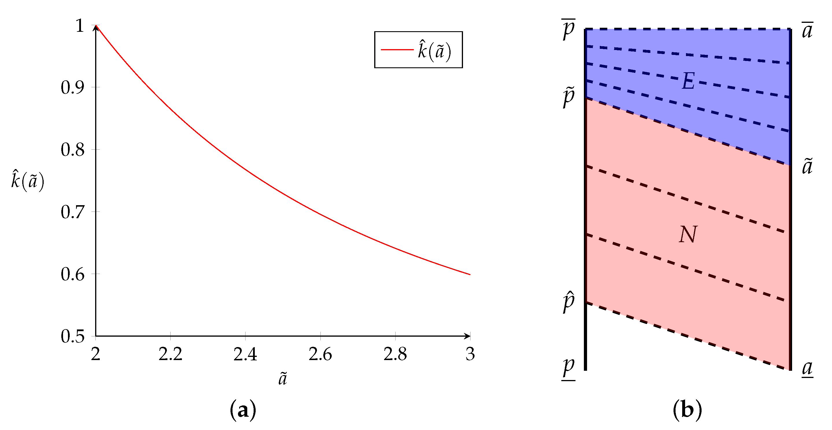
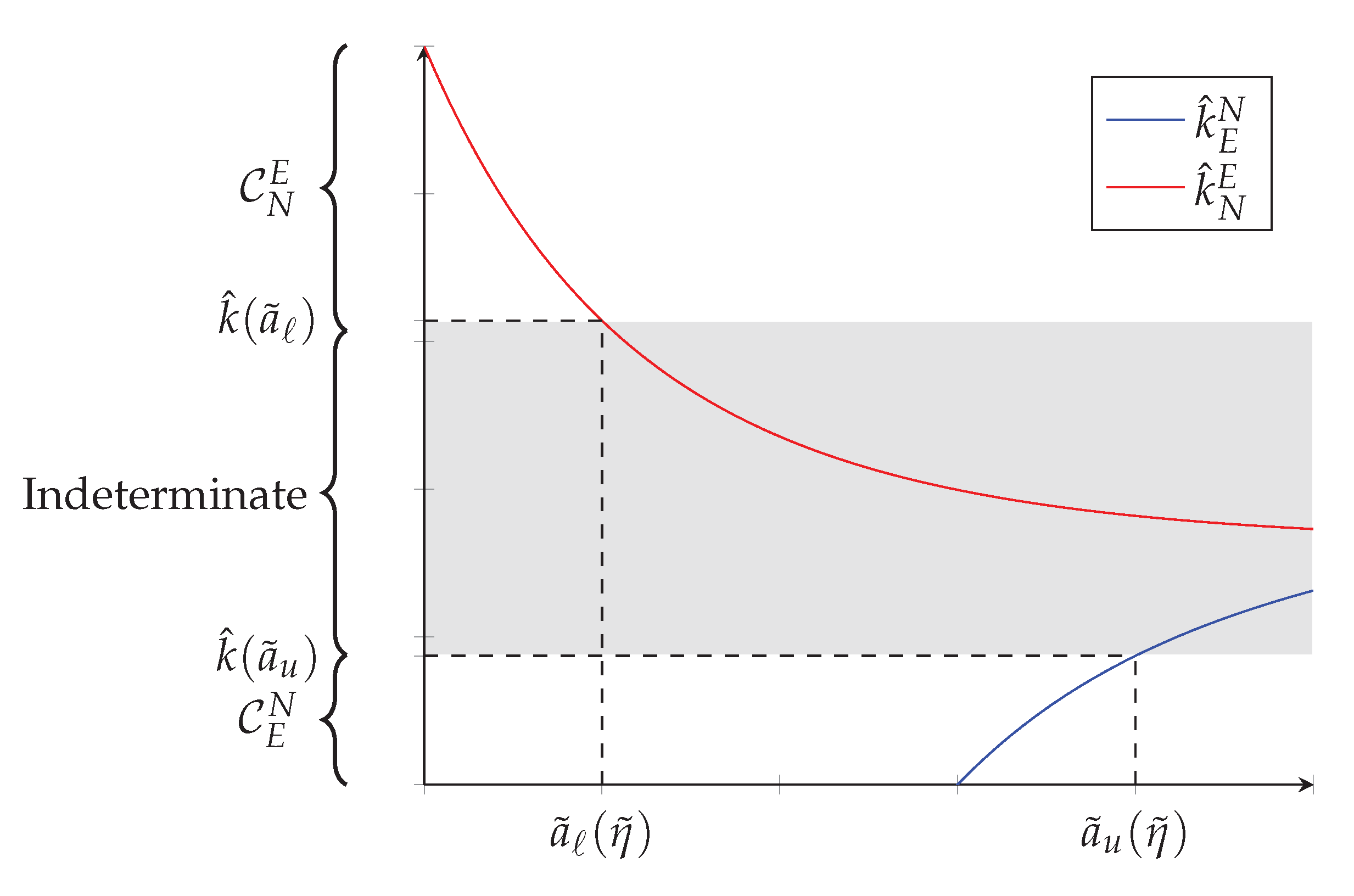
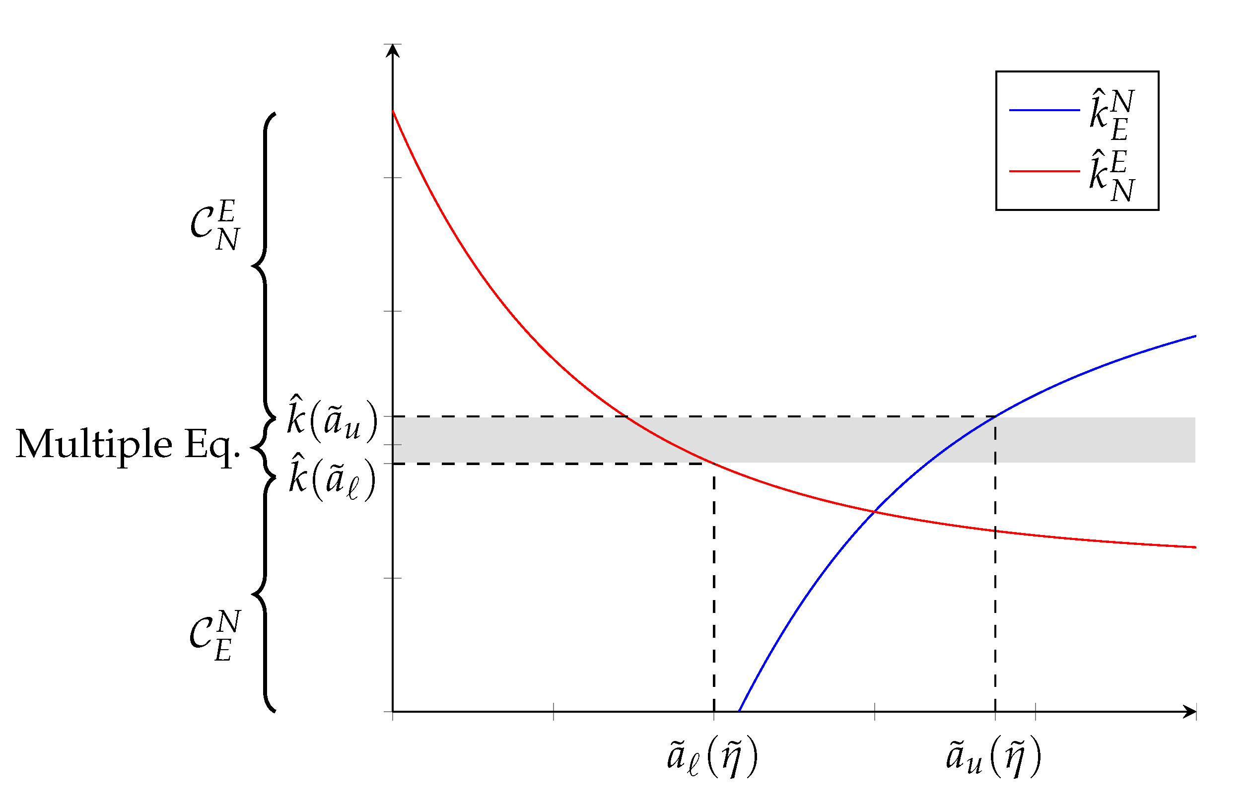
Next, I examine the conditions for a contract switch to occur using a simple example. Panel (a) of Figure 2 depicts the threshold function for productivity types distributed uniformly over with and . Now, small values of k will result in only nonexclusive contracts being signed, and large values of k will induce a contract switch.16 The intuition is that agents are only productive enough to offset the endogenous outside option of the principal when cost inefficiencies are sufficiently small. Panel (b) of Figure 2 shows a potential contract pattern that can be obtained under Proposition 3, when cost inefficiencies are small enough for a contract switch to occur. Now there are principals left out of the market. I denote the lowest type principal that is matched with an agent by , so that principals of type remain unemployed under the equilibrium assignment.
The previous example where k is a per unit usage cost is still applicable, but now there are many principals competing for the services of a small number of agents. The reduction in leverage for the principals coming from a less appealing outside option leads them to sign nonexclusive contracts even in the presence of sizable effort inefficiencies. In this case, , which implies that no exclusive contracts will be signed if effort inefficiencies lead to a reduction in surplus no greater than .
Now, I provide a proposition analogous to Proposition 2 from the previous section.
Proposition 4.
If , then the stable matching is or .
Proof.
See Appendix A.5. □
Corollary 2.
there is no stable matching pattern when .
Similarly to Proposition 2, the implication from Proposition 4 is that a single interval exists for values of k that support or as stable contract patterns. Corollary 2 states that when k is smaller than the infimum of the set K, the LNDC is not robust to global deviations, which in turn implies that the contract pattern is not stable.
5.3. Utility Functions
Now, I consider the utility functions that arise under the two cases described in Propositions 1 and 3. I focus on the cases where the market exhibits contract switching. I examine the effects of a change in k on the utility functions, and the differential effect on agents. In all cases, I denote derivatives with subscripts. Before moving on, it is important to discuss the constants of integration for nonexclusive contracts, after which I present a claim that is helpful moving forward.
While the nonexclusive contract ODE in (13) determines the slope of the utility function contributed by each principal, it is feasible for the constant of integration to be any convex combination of the total utility accruing to the lowest type of agent matched in a nonexclusive contract. When there is principal unemployment each principal contributes the entirety of the surplus to the match, so the constants of integration are easily determined. In the case of agent unemployment, the lowest type of agent matched in a nonexclusive contract is at the marginal coalition. Consequently, the total utility they receive is equal to the exclusive contract utility at the marginal coalition and must be split between the two principals. It is possible to determine how the utility will be split using the individual rationality constraints of the principals, and thus pin down the constants of integration. Thus, we have the following claim:
Claim 1.
For each set of nonexclusive contract utilities, and , the constants of integration are pinned down for all possible contract patterns.
Proof.
See Appendix A.6. □
Claim 1 implies that no additional assumptions are required in order to determine the equilibrium utility functions under nonexclusive contracts, which precludes the need to define a sharing rule that could jeopardize the stability of the matching market.
5.3.1. Agent Unemployment
In this case, the contract pattern in the market is . First, consider the nonexclusive utility functions for a pair of principals, and , that are matched to agent a:
when , the utility function will just be . Thus, after summing (37) and (38), the entire utility function can be written as follows:
Now, I examine the effect an increase in k has on the utility function. I consider three cases. First, the effect on agents signing exclusive contracts before and after the change, then the effect on agents in nonexclusive contracts before and after the change, and last, the effect on agents transitioning from one contract to the other.
Exclusive Contract Utility:
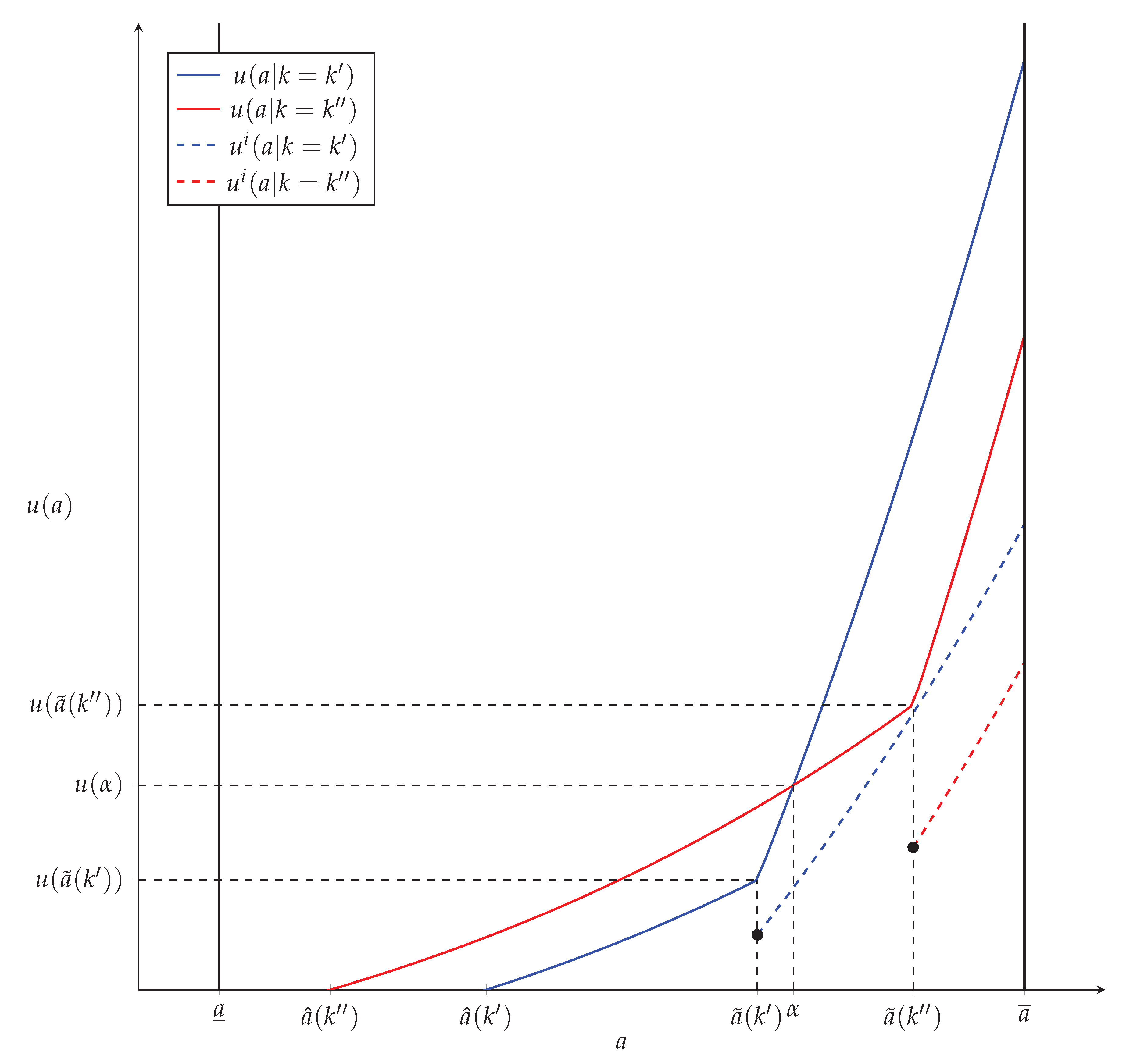
The second term in (40) is negative, because and . Therefore, the entire term is positive. Also, note that only the indirect effect is present in this expression, since the exclusive contract is only a function of the cost inefficiency through its impact on the productivity type marginal coalition. This result is not surprising, because an increase in k leads to fewer agents remaining unmatched at the bottom of the type distribution. Thus, the agents below the threshold gain bargaining power. Consider Figure 3 to see that this effect is the most obvious for the lowest type of agent in the market before the change in k. This agent, , receives a utility increase equal to . Here, denotes the lowest type of agent in the market when .17 Additionally, represents the portion of the nonexclusive utility function that is paid by principal i.
Nonexclusive Contract Utility:
The derivative with respect to k is as follows:
Here, I drop the superscripts designating principals to indicate the total nonexclusive utility. The direct effect in (41) is negative, since the profit from the nonexclusive contract is decreasing in k. For all the agents that remain in nonexclusive contracts after an increase in k, the direct effect outweighs the indirect effect. Thus, these agents receive a lower compensation when k increases.
Contract Switching:
Now consider the case where an agent switches from a nonexclusive to an exclusive contract. These are those with types between and in Figure 3. I denote the agent equally well off under either value of k by . Agents of type benefit from this increase in k due to agent entry at the bottom driving up the exclusive contract utility they can command. The agents of type actually become worse off, because the slope of the nonexclusive portion of the original utility function offsets the gain from increased bargaining power for the agents. The value of the agent of type is determined by the size of the change in k, and the curvature of the exclusive and nonexclusive portions of the utility function.
5.3.2. Principal Unemployment
In this case, the constant of integration is no longer zero. Consider the nonexclusive utility functions, which obtain the following for :
The entire utility function is the sum of Equations (42) and (43), and the exclusive utility function is evaluated for agents . This can be written compactly as follows:
I now examine how changes in k affect the utility function. I consider the effects on agents remaining in nonexclusive contracts and those remaining in exclusive contracts.
Nonexclusive Contract Utility:
Exclusive Contract Utility:
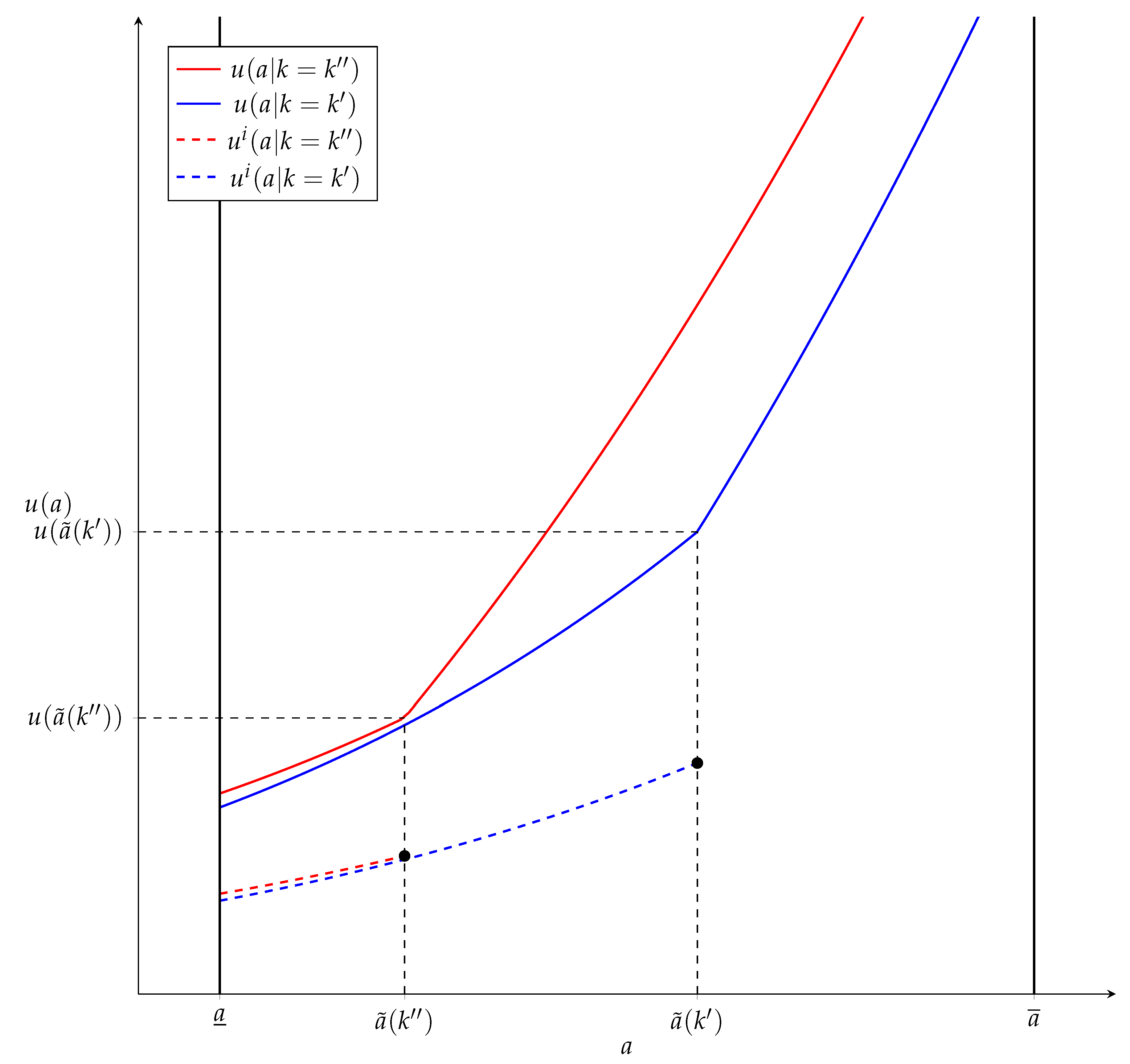
In both cases, the indirect effect dominates the direct effect. Thus, utilities are increasing in k, which seems counterintuitive as it is a source of inefficiency in the model. The effect comes entirely from the principal exit that occurs when k increases. As more agents sign exclusive contracts, more principals are forced out of the market, and agents match with more productive principals.
Figure 4 shows that the size of this increase depends on which contract an agent signs before and after the change in k.
6. Implications
There are both inter- and intraorganizational examples for which the current framework has particularly important implications. In the case of an intraorganizational matching market, the equilibrium outcome can be viewed as the solution to the problem facing a manager in which they must match two sets of workers to perform tasks. The CPOME guarantees the equilibrium will be the same as if the manager had allowed workers in the two sets to choose match partners themselves.
Consider a case in which the manager must assign teams of product developers to teams of sales associates. In this example, there are likely to be more sales teams than product development teams. The inefficiency cost represents the additional product knowledge sales teams must obtain in order to sell products for multiple development teams. In practice, this additional knowledge requirement may lead to teams dividing into subgroups with each subgroup focusing on one particular project. The inefficiency arises from the reduced number of salespeople per project, which increases the effort costs. Given the analyses in Section 5.2.2 and Section 5.3.1, when inefficiency costs are sufficiently small, the manager will assign some of the more productive sales teams to two development teams. Suppose there is a positive, exogenous shock to the inefficiency parameter, k. One example of such a shock could be the increase in complexity of the products the company makes, which in turn requires more working knowledge to sell effectively.18 In response, the manager will optimally choose to reallocate sales teams within the firm by reducing the number of teams that sell multiple products. The manager will also look to hire salespeople from outside of the firm in order to have enough sales teams to pair with product development teams. In addition to the firm organizational decisions, the model also makes a prediction related to output. More specifically, unemployment will decrease in response to a decrease in output. This result is particularly puzzling but has a relatively simple explanation. A reduction in worker efficiency necessarily decreases output, but it is worse to leave product development teams idle after reallocating sales teams than it is to hire lower quality sales teams with whom the idle development teams can partner.
Now consider an example in which there are more principals than agents. Suppose a large firm has a limited number of plants that are needed to produce goods developed by many different divisions. Again, we can equate the optimal assignment of plants to divisions by a social-planner-style authority within the firm to the equilibrium outcome of an intrafirm matching market where plant managers contract with division heads. In this case, plant managers can agree to produce products for up to two divisions at the same time, but outfitting a plant to simultaneously produce different goods incurs additional costs. These costs include more worker training and reduced space/time for the production of each individual good. Consider a case in which inefficiency costs are sufficiently small, so all plants produce goods for two divisions. Suppose the firm suffers a technological malfunction across plants that inhibits their ability to produce multiple goods simultaneously. This represents a positive inefficiency cost shock. As a result of increased inefficiency costs, the central authority within the firm finds it optimal to reallocate production, so that some of the most productive plants only produce a single good. A consequence of this reallocation is that a number of the less profitable products will not be produced in the short term.19 Essentially, the firm optimally stops production for some goods until either the malfunction is repaired or more plants are built.
7. Conclusions
The present paper seeks to extend the two-sided matching literature with multiple contracts to a many-to-one setting. I achieve this by introducing nonexclusive contracting into a two-sided matching framework, which allows me to provide a theoretical basis for the coexistence of exclusive and nonexclusive contracts within the same market. I find that endogenizing the outside option and cost-sharing between principals are essential to obtaining this result, and without the two forces, no contract switching would occur. I show that the relative measure of principals to agents is essential for determining the type of contract patterns that can arise in a given market. Thus, all three forces are essential for generating theoretical results that mirror market conditions in a number of industries. Recall that if one of these three facets of the model is missing, then the results can be completely different. It is important to mention that these contract patterns arise with PAM obtaining for either contract type. Additionally, I show that the contract pattern is monotonic, since a market only exhibits a single switching point if both contracts coexist. It is uncertain how the results will change if one uses a model similar to [9], in which the equilibrium matching may exhibit NAM, and the surplus function from a match is not linear in the cost inefficiency term k. However, I leave this analysis for future research.
Potential future work includes examining contract patterns that arise when there is a moral hazard in the contracting problem. This will make it possible to understand how incentives in nonexclusive contracts are affected by an endogenous outside option, which I have shown is vital to the results in the model. Another possible extension is adapting the model to allow for up to principals to contract with a single agent. This addition would make the model more realistic, but the results may not add enough relative to the current paper to justify the difficulty. If the functional forms are similar, I would expect contract patterns to remain monotonic, and thus not add much in the way of new results. Finally, it could be interesting to see how the results change if agents are heterogeneous in the effort inefficiency term, so that matching occurs between principals with some productivity or project value and agents that differ in their ability to multitask.
Funding
This research received no external funding.
Data Availability Statement
No new data were created or analyzed in this study. Data sharing is not applicable to this article.
Acknowledgments
I would like to thank Konstantinos Serfes for his support, advice, and many helpful conversations, as well as, Mian Dai, Kaniska Dam, and Ricardo Serrano-Padial for helpful comments. As always, all remaining errors are my own.
Conflicts of Interest
The authors declare no conflict of interest.
Appendix A. Proofs
Proofs The proofs for Propositions 2 through 5 are done using the functional form , but the argument holds for any function that is multiplicatively separable in a and p.
Appendix A.1. Second-Order Conditions
First, I show that if the SOCs are satisfied, then it is possible for PAM to obtain. Before I continue, it is important to note that the FOCs and SOCs for each principal must be satisfied, but their problems are identical, so I focus on the problem of principal i. The FOC evaluated at the optimal assignment:
Differentiating (A1) in order to obtain the SOC for principal i, and suppressing function arguments for exposition:
The corresponding SOC for principal j is
Appendix A.2
Proof of Proposition 1.
If , then the potential contract patterns are and . In this case, no principal will ever be left out of the market even if all the contracts are exclusive. Thus, the principal at the bottom of the market, , has all the bargaining power. Therefore, in either contract, the principal will offer a utility of zero to the lowest potential agent they could match with, which I denote . The principal must then choose between:
The principal will choose the exclusive contract as long as . □
Appendix A.3
Proof of Proposition 2.
I proceed by considering the potential deviations of principals and agents and then derive conditions for which none of the deviations will be profitable. Here, there are two potential contract patterns, and . There is a local nondeviation condition:
Recall that this condition only considers deviations by a principal–agent pair to a different contract. At some marginal coalition, this condition holds with equality. The condition can be rewritten as
The term is the lowest type of agent that is matched when the marginal coalition is . Since this condition is local, there are additional deviations that must be considered in order to ensure stability.
- Above the Marginal Coalition:
First, I consider a deviation by types above the marginal coalition. In the current case, these coalitions will sign nonexclusive contracts on the equilibrium path. The deviation I consider is by a principal, to sign an exclusive contract with an agent of type a, where . I denote this deviation as . The payoff to principal on equilibrium is
The second inequality in (A6) comes from standard increasing differences, while the last inequality comes from the fact that the total nonexclusive utility is what the agent would obtain in equilibrium, and it is larger than the exclusive utility above the marginal coalition. Thus, the deviation is not profitable for principal .
- Below the Marginal Coalition:
Now, I examine potential deviations below the marginal coalition. Here, I use . Below the marginal coalition, principal–agent pairs will sign exclusive contracts on the equilibrium path. Consider the following deviation:
In order for this to be nonprofitable, the following must hold:
Differentiating this with respect to a gives , which implies the condition will be most difficult to satisfy when . Thus, the deviation is never more profitable than a local deviation across contracts. Therefore, it is never profitable under (A5).
Next, consider the deviation below:
In order for this to be nonprofitable, the following must hold:
Here, denotes the principal pair . The inequality in (A11) can be rearranged to give
Differentiating this with respect to a gives , which implies the condition will be most difficult to satisfy when . Again, this implies (A10) will never be more profitable than a local deviation across contracts.
Next, consider the following deviation:
For (A13) to be unprofitable the inequality below must hold:
This can be rearranged to obtain
Differentiating this with respect to a gives , which implies the condition will be most difficult to satisfy when . Now, rearrange (A14) and evaluate at the optimal assignment and at :
The inequality in (A16) holds with equality when . For exposition, I now write as a, so that (A16) at the equilibrium assignment becomes
Since (A17) holds with equality at , it must be strict for . This requires the slope with respect to a of the negative terms in (A17) to be larger than the positive terms. This way, there is a single crossing that occurs at . The terms affected by changes in a are and . The single crossing will only ensure (A17) holds if both of these terms are convex or concave in a. If is concave, and is convex, then (A17) will not hold. The first and second derivatives of are
If is convex, then the function is convex. If it is concave, then
must hold in order for the function to be convex. A similar result is obtained for . Again, if is convex, then the function is convex. If it is concave, then
must hold for the function to be convex. Notice that if (A19) holds, then (A20) will necessarily hold. Given that both of these terms are convex, all that must be done is to confirm that the single crossing holds at . The inequality that must be satisfied is
After some simplification (A21) becomes
Remember that this must be evaluated at . Additionally, the LHS of (A22) will be on the equilibrium path. Thus, (A22) becomes
Rearranging (A23) gives
If both terms are convex, and (A24) holds, then the deviation is not profitable. The next step is to show that (A24) will hold for different values of . Since when (i.e., when only nonexclusive contracts are signed), (A24) will hold for . If , then (A24) will hold for every . If , then there are two possibilities. First, it could be that
This implies that (A23) will hold and the deviation will be unprofitable. The other case is that (A23) will be violated for some . Thus, for every the deviation will be unprofitable, but for every , the deviation will be profitable. This would result in the contract pattern being unstable.
- Across the Marginal Coalition:
Now, I consider deviations across the marginal coalition. Here, I use . First, I examine the deviation below:
In order for (A26) to be unprofitable, the inequality below must hold:
The RHS of (A27) is increasing in i faster than the LHS. Thus, the inequality is most difficult to satisfy when , so (A27) becomes
This inequality is most difficult to satisfy at , which leads to (A28) holding with equality. Therefore, it is never violated, and (A26) is unprofitable.
The next deviation I consider is
This deviation will be unprofitable if the following holds:
The first inequality comes from the increasing difference conditions within contracts. The second inequality comes from the fact that the equilibrium utility, , below the cutoff is larger than the nonexclusive utility below the cutoff. Thus, the principal pair would prefer the equilibrium assignment to a deviating coalition with a.
Now consider the following deviation:
In order for (A31) to be unprofitable, the following must hold:
Differentiating (A32) with respect to along the equilibrium assignment gives
This implies that (A31) will be most difficult to satisfy when . Rearrange (A33) and evaluate at the optimal assignment and :
Next, I examine the deviation below:
This will not be profitable if the inequality below holds:
Since , (A35) is most difficult to satisfy at . The condition then becomes identical to (A10), which has already been shown to hold.
The last deviation I consider is
This not profitable when
Appendix A.4
Proof of Proposition 3.
If , then the potential contract patterns are and . This result comes from the fact that even if all coalitions sign nonexclusive contracts, no agents will ever be left out of the market. This gives the agent at the bottom of the market all the bargaining power. Let this agent be denoted by . The agent will receive an exclusive contract offer of , where is the lowest type principal potentially matched with . The nonexclusive contract offer will be , where i and j represent two principals of type . In the current setting, the contract offers are as follows:
Clearly, the nonexclusive contract offer will be favored as long as . □
Appendix A.5
Proof of Proposition 4.
The approach here is similar to the one used for Proposition 2. I examine the potential deviations and derive conditions that ensure these deviations will not be profitable. I start with the following inequality, which I call (A39):
At some marginal principal–agent pair , this condition holds with equality. Plugging in the function forms, and solving for k gives
For a given k, all will match in an exclusive contract, and all will match in nonexclusive contracts. This condition makes it possible to identify deviations across contracts by principals above or below the marginal principal, .
The first deviation I consider involves a principal below the cutoff, j, deviating to a principal–agent pair above the cutoff, , and entering a nonexclusive contract. This deviation will not be profitable if it satisfies the following inequality, which I call the Global Nondeviation Condition, or GNDC
where a is the agent type to which the principal of type j is matched. The GNDC simply states that the remaining surplus from the deviating coalition contract when keeping and j equally well off must be less than the surplus apportioned to from the coalition contract . The GNDC can be rewritten by plugging in the matching functions for each contract to give
The implicit assumption here is that . Since (A43) must hold for each and , the minimum k that will satisfy (A43) must be larger than the maximum value of for each argument. In order to simplify the expression, consider how changes as a changes
where D is the denominator from (A43). Clearly, (A44) is positive whenever , which implies that maximizes the function for any . Therefore, as long as for every the GNDC will be satisfied for that value of k. There are two additional deviations that must be considered before being able to categorize the conditions that will ensure is a stable matching. The first considers a similar deviation to the GNDC, where the only difference is that deviates down to . This condition can be simplified to the following expression
Differentiating the RHS of (A45) with respect to a, we obtain
which implies that for a given the RHS will be largest when . Thus, we can replace a in (A45) with . Additionally, at the marginal coalition, (A45) is satisfied with equality. In order to see whether or not the inequality is satisfied for each , differentiate (A45) with respect to with to obtain
From the FOC of the matching stage, we know that the first and third terms on the LHS of (A46) are equal, so (A46) simplifies to
Clearly, (A47) is satisfied under the current function form. The next deviation to consider is i deviating from to . This will not be profitable if the following holds
Again, this will hold with equality at the marginal coalition, and from the FOC we know that the RHS differentiated with respect to is negative, because . Therefore, (A48) will hold for each . Now that all the deviations across the threshold have been considered, it is possible to define a condition that ensures is a stable matching. The condition will be a combination of the LNDC2 and the GNDC. The LNDC2 gives the coalition at which a switch will occur if it is stable. As long as the k inducing the switching point does not violate the GNDC for the coalitions above the marginal coalition, then the matching will be stable. Since is fixed for all , only changes as changes. Thus, must hold for each .
Now, I find the conditions necessary to ensure the existence of the set K in general. First, I introduce the conditions to be satisfied in order for a given k to be an element of the set K.
If , then the following hold:
Since the threshold function, , is a bijective function on the domain of the type distribution of the agents, condition 1 will hold if such a set K exists.
I need to show when condition 2 will hold and that the set K is unique. I perform this in the following steps:
- First, I show when condition 2 will hold.
- Then, I express the requirements for condition 2 to hold as a restriction on the exclusive matching function.
- Finally, I derive conditions for the set K to be unique.
- Step One:
Note that at , so in order for condition 2 to hold, it must be that . Additionally, when the derivative is negative at the marginal coalition, it must be that it does not become positive as increases and leads to crossing from below. Thus, if the derivative is nonincreasing in when it is negative at the marginal coalition, then and will never cross. The derivative of with respect to after some simplification is
Rearranging and canceling gives me the following inequality:
where . If the LHS of (A50) is increasing in faster than the RHS, then this inequality will hold for all . Since the RHS is not a function of , The LHS just needs to be increasing in . The derivative of the LHS with respect to after simplification is
The expression in (A51) is necessarily positive as long as the exclusive matching function is nonconcave. If it is concave, then the following condition must hold:
When (A51) holds, will be nonincreasing in when the derivative is negative at , if . This implies that the stability condition will be satisfied for a given . Note that the sign of the derivative will be positive or negative depending on the value of . The values of for which the derivative is negative correspond to the values of that satisfy the stability condition.
- Step One:
For a stability condition in terms of the exclusive matching function, (A49) can be rearranged to give
By Grönwall’s Lemma, is bounded below by the solution to the RHS of (A53), which I call . Thus, the ODE for the lower bound of the matching function is
The solution to (A54) is
Since the sign of the derivative evaluated at determines whether the matching is stable, the following condition will give a stable matching with at switching point at :
The second condition is satisfied when (A52) and (A56) are both satisfied. When both are satisfied, K is necessarily nonempty, and the stable matching is .
- Step Three (Interval Uniqueness):
Since (A56) is for a single , it must be shown that there is an interval for which it is satisfied and that this interval is unique.
First, consider the when , which is the lowest possible lower bound for the interval. If this is plugged into the condition on the derivative of the matching function
Since the slope of the matching function, is always positive under PAM, this condition is satisfied at the lower bound. Therefore, the lower bound of the interval is the same as the lower bound of the distribution.
Now, the uniqueness of the interval must be determined. If the interval is unique, then the upper bound of the interval can be found by setting , and solving for . It is then possible to find the value of by using (A54) and (A55). This is performed by evaluating (A54) and (A55) at the upper bound, , and plugging (A55) into (A54). It is then simple to solve for the value of . This makes it possible to show that (A56) is satisfied. This will only work if the interval is unique.
Since the sign of will be positive when the stability condition is violated, it must be that the sign is positive for every in order for the interval to be unique. This will be true if is nondecreasing in . Thus, taking the derivative with respect to gives
where . Again, (A58) must be evaluated at the marginal coalition, which gives the following after some simplification:
The expression in (A59) is always positive due to the sign of and . The first term is always positive since it is the slope of the nonexclusive matching function at the marginal coalition. The second term is negative, because the principal type matched with a given agent is decreasing as the type of the marginal coalition increases. Therefore, (A59) is always positive when , so the interval of stable marginal coalitions is unique. □
Appendix A.6
Proof of Claim 1.
The utility functions for each principal are as follows:
The constants of integration must be such that , which simply states that they must be equal to the outside option for the lowest type of agent. The outside option of the lowest type of agent in a nonexclusive coalition will depend on the contract pattern that obtains in the market.
Just as in the original model, there are four possible contract types that depend on the relative measure of principals and agents. When , the two potential contract patterns are and . When the two potential contract patterns are and .
I start with the second case, since it is simpler. In this case, there will be principals left out of the market. The lowest type principals will offer the agent all of the surplus they generate when matched under a nonexclusive contract, since the outside option for the agent is a nonexclusive contract with the two highest type principals left out of the market. This means that the principals will offer
Therefore, the constants of integration are easily determined for this case.
Now consider the case where . In this setting, the lowest principals in a nonexclusive contract must offer the agent a total utility equal to the exclusive utility the agent could receive if the agent rejected the nonexclusive contract. Thus, the constants of integration must be such that
At first glance, it seems as though the constants of integration will not be determined, however, that is not true. Recall the individual rationality constraints for each principal, these two constraints can be used to pin down the constants of integration. First, consider the constraint for principal i for the marginal coalition
Equation (A64) can be used to solve for an upper bound on
Similarly, the upper bound for principal j is
Now consider a lower bound on . Principal i will never pay more than enough to ensure the agent prefers the nonexclusive contract. The smallest this value will ever be is when principal j pays . Thus, the lower bounds for each agent are
and
This gives the following utility intervals for each principal
The utilities will be pinned down when this interval collapses to a single point, which can be found be when the difference in the bounds is equal to zero. Consider this point for principal i
Notice that the last equality is the same as the condition for the nonexclusive contract to be preferred at the marginal coalition. Thus, the utility can be pinned down using the expression for the upper bound of the utility interval. The utilities for each principal are as follows:
Therefore, the constants of integration are determined in this case, which means that they are always determined no matter which type of contract obtains in the market. □
Appendix B. Numerical Example
Here, I provide a numerical example to give some intuition. Let p and a represent the principal and agent types, respectively, where . The distribution for the agents is , and the distribution for the principals is . Additionally, let the density of principals be twice that of the agents. The exclusive matching function in this case is . The nonexclusive matching function is .
The threshold function in this example is
I need to show that the stability condition on the matching function holds for this example. When evaluated at the upper bound of the stable interval, , the inequality in (A53) will become an equality. This can then be used to solve for the upper bound, which in this case is . I can now find the constant from (A55) by plugging into the stability condition and setting the two functions equal to each other like below:
In the current example, this gives
If this is plugged back into the stability condition, it is possible to plot both functions to show that the condition is satisfied for a unique interval , which is . In Figure A1 below, the blue and red lines correspond to the LHS and RHS of (A56), respectively.
Figure A2 shows the threshold function where the set K is the interval . The dashed red portion of the threshold function indicates pairs that do not induce a stable matching.
Figure A1.
Stability Condition.

Figure A2.
Threshold Function.

Appendix C. General Matching Functions
Appendix C.1. Matching Functions
Let the measure of principals and agents be and , respectively. The ratio of the measures is then . Also, let and denote the distributions for principals and agents, respectively.
: The measure preserving property in each case is
: The measure preserving property in each case is
Appendix C.2. Contract Patterns
: In this case, principals will be left out of the market. In order for that to happen for a given measure of each contract the following inequality must hold
In (A82), represents the measure of agents signing contract x. For a given , there will be a marginal agent, , where (A82) holds with equality. For all of the , cannot be obtained as a contract pattern. This marginal agent can be written as .
: In this case, agents will be left out of the market. In order for that to happen for a given measure of each contract the following inequality must hold:
where is the measure of agents that are unmatched. For a given , there is a marginal agent, , such that (A83) holds with equality. For all of the , cannot be obtained as a contract pattern. This marginal agent can be written as .
There are two possible cases regarding these marginal agents. They are and . Figure A3 depicts the first case, in which there is no overlap of the contract patterns for a given k. Instead there is a region, , , where the contract pattern is indeterminate.
In Figure A4, there is a region, , , where both contract patterns are possible.
We must determine whether or not this case can arise, and if so, the conditions necessary to guarantee it will obtain. First, this requires determining and .
Figure A3.
Indeterminacy.

Figure A4.
Multiplicity.

The other threshold function is
If the case where obtaining multiple equilibria is possible, then it must be that (A85) is greater than (A86) for some . Setting (A85) greater than (A86) and simplifying we obtain
Plugging and into the matching functions gives
At the respective marginal coalitions
Equation (A92) can also be written as
Notice that (A93) is a function of and the lower bounds for the distributions of principal and agents.
| 1 | A contract pattern is monotonic if there is no more than one point in the type distributions of the principals and agents where the type of contract signed changes. |
| 2 | Here, I use the subscripts i and j to distinguish between two principals of the same productivity type. As will become clear after the analysis of the contracting problem, I only need to examine a principal-agent pair, because principal j’s type does not enter into the problem for principal i. |
| 3 | One could imagine a cost function of the form , where effort exerted for each principal is impacted by effort exerted for the other. The effort externality causes stability issues in the matching market when there are a continuum of types. |
| 4 | In Section 3.3 I will solve the contracting problem for a principal-agent pair. |
| 5 | Initial work on a model with moral hazard found that the result regarding the monotonicity of contract patterns was not affected by incentive contracts alone. In order to have nonmonotonicity, the model must have a limited liability constraint that binds for some principal-agent pairs and not for others. |
| 6 | I will discuss the bargaining frontier in greater detail in Section 4. |
| 7 | I leave an in depth discussion of the utility functions for Section 5. |
| 8 | This is just the sum of the utilities received from the principals entering nonexclusive contracts with the agent, so that . |
| 9 | Definitions 3 and 4 are borrowed from [11], and altered to fit my model. |
| 10 | In their setting with colleges and students, a college’s preferences over a set of students is responsive to its preferences over individual students, if there are two matchings that differ only by two students, and the college prefers the set containing the more preferred student. Consider a preference ranking for an agent in my model, where . The agent’s preferences are responsive if . |
| 11 | It is important to note that in the model , because no more than two principals can match with an agent. |
| 12 | Recall, the total surplus generated by a principal-agent coalition under a nonexclusive contract is just the sum of the surpluses generated by the two principals matched with a given agent. For example, . |
| 13 | Since it is a local condition, satisfying the (26) does not ensure the equilibrium is pairwise stable. Thus I say I evaluate at a proposed equilibrium assignment and not a stable equilibrium assignment . |
| 14 | If we do not make this change, then differentiating both sides of the inequality with respect to agent productivity type incorrectly readjusts the relevant principal type in the nonexclusive surplus function. |
| 15 | Note that these are potential contracts, and they may or may not be stable. |
| 16 | Note that these are potential contracts, and they may or may not be stable. |
| 17 | This is a slight abuse of notation, since it is technically , but is suppressed for exposition. |
| 18 | The underlying assumption is that the increased complexity does not lead to increased revenue. This could be due to all firms adopting a new innovation, and an intensely competitive market structure preventing firms from gaining an advantage. |
| 19 | The matching market can be thought of as a short-term problem that is solved each period. Eventually it may be optimal for the firm to build more plants, which would change the assignment problem. |
References
- Marvel, H.P. Exclusive Dealing. J. Law Econ. 1982, 25, 64–103. [Google Scholar] [CrossRef]
- Sass, T.R.; Gisser, M. Agency Cost, Firm Size, and Exclusive Dealing. J. Law Econ. 1989, 32, 381–400. [Google Scholar] [CrossRef]
- von Lilienfeld-Toal, U.; Mookherjee, D. A General Equilibrium Analysis of Personal Bankruptcy Law. Economica 2016, 83, 31–58. [Google Scholar] [CrossRef]
- Parlour, C.A.; Rajan, U. Competition in Loan Contracts. Am. Econ. Rev. 2001, 91, 1311–1328. [Google Scholar] [CrossRef]
- Matouschek, N.; Ramezzana, P. The Role Of Exclusive Contracts In Facilitating Market Transactions. J. Ind. Econ. 2007, 55, 347–371. [Google Scholar] [CrossRef]
- Sass, T.R. The competitive effects of exclusive dealing: Evidence from the U.S. beer industry. Int. J. Ind. Organ. 2005, 23, 203–225. [Google Scholar] [CrossRef]
- Besley, T.; Ghatak, M. Competition and Incentives with Motivated Agents. Am. Econ. Rev. 2005, 95, 616–636. [Google Scholar] [CrossRef]
- Dam, K.; Pérez-Castrillo, D. The Principal-Agent Matching Market. Front. Theor. Econ. 2006, 2, 20021001. [Google Scholar] [CrossRef]
- Serfes, K. Endogenous Matching in a Market with Heterogeneous Principals and Agents. Int. J. Game Theory 2008, 36, 587–619. [Google Scholar] [CrossRef]
- Dam, K.; Ripperger-Suhler, D.; Serfes, K. Two-sided productivity heterogeneity, firm boundaries, and assortative matching. J. Econ. Manag. Strategy, 2023; in press. [Google Scholar]
- Alonso-Paulí, E.; Pérez-Castrillo, D. Codes of Best Practice in Competitive Markets for Managers. Econ. Theory 2012, 49, 113–141. [Google Scholar] [CrossRef]
- Macho-Stadler, I.; Pérez-Castrillo, D.; Porteiro, N. Coexistence of Long-term and Short-term Contracts. Games Econ. Behav. 2014, 86, 145–164. [Google Scholar] [CrossRef]
- Hatfield, J.; Milgrom, P. Matching with Contracts. Am. Econ. Rev. 2005, 95, 913–935. [Google Scholar] [CrossRef]
- Kelso, A.S.; Crawford, V.P. Job Matching, Coalition Formation, and Gross Substitutes. Econometrica 1982, 50, 1483–1504. [Google Scholar] [CrossRef]
- Hatfield, J.W.; Kojima, F. Substitutes and Stability for Matching with Contracts. J. Econ. Theory 2010, 145, 1704–1723. [Google Scholar] [CrossRef]
- Azevedo, E.M. Imperfect Competition in Two-Sided Matching Markets. Games Econ. Behav. 2014, 83, 207–223. [Google Scholar] [CrossRef]
- Eeckhout, J.; Kircher, P. Assortative Matching with Large Firms. Econometrica 2018, 86, 85–132. [Google Scholar] [CrossRef]
- Maier, N.; Ottaviani, M. Information Sharing in Common Agency: When is Transparency Good? J. Eur. Econ. Assoc. 2009, 7, 162–187. [Google Scholar] [CrossRef]
- Holmstrom, B.; Milgrom, P. Common Agency and Exclusive Dealing; Working Paper; Yale University, School of Management: New Haven, CT, USA, 1988. [Google Scholar]
- Holmstrom, B.; Milgrom, P. Multitask Principal-Agent Analyses: Incentive Contracts, Asset Ownership, and Job Design. J. Law Econ. Organ. 1991, 7, 24–52. [Google Scholar] [CrossRef]
- Dutta, B.; Masso, J. Stability of Matchings When Individuals Have Preferences over Colleagues. J. Econ. Theory 1997, 75, 464–475. [Google Scholar] [CrossRef]
- Roth, A.E.; Sotomayor, M. Two-Sided Matching: A Study in Game-Theoretic Modeling and Analysis; Wiley: Hoboken, NJ, USA, 1990. [Google Scholar]
Figure 1.
More Agents Than Principals. (a) Threshold Function. (b) Contract Pattern.

Figure 2.
More Principals Than Agents. (a) Threshold Function. (b) Contract Pattern.

Figure 3.
Utility Functions ().

Figure 4.
Utility Functions ().

Disclaimer/Publisher’s Note: The statements, opinions and data contained in all publications are solely those of the individual author(s) and contributor(s) and not of MDPI and/or the editor(s). MDPI and/or the editor(s) disclaim responsibility for any injury to people or property resulting from any ideas, methods, instructions or products referred to in the content. |
© 2024 by the author. Licensee MDPI, Basel, Switzerland. This article is an open access article distributed under the terms and conditions of the Creative Commons Attribution (CC BY) license (https://creativecommons.org/licenses/by/4.0/).
Share and Cite
MDPI and ACS Style
Ripperger-Suhler, D. Matching with Nonexclusive Contracts. Games 2024, 15, 11. https://doi.org/10.3390/g15020011
AMA Style
Ripperger-Suhler D. Matching with Nonexclusive Contracts. Games. 2024; 15(2):11. https://doi.org/10.3390/g15020011
Chicago/Turabian StyleRipperger-Suhler, Daniel. 2024. "Matching with Nonexclusive Contracts" Games 15, no. 2: 11. https://doi.org/10.3390/g15020011
Note that from the first issue of 2016, this journal uses article numbers instead of page numbers. See further details here.