A New Approach to Multiroot Vectorial Problems: Highly Efficient Parallel Computing Schemes

Abstract

In this article, we construct an efficient family of simultaneous methods for finding all the distinct as well as multiple roots of polynomial equations. Convergence analysis proves that the order of convergence of newly constructed family of simultaneous methods is seventeen. Fractal-based simultaneous iterative algorithms are thoroughly examined. Using self-similar features, fractal-based simultaneous schemes can converge to solutions faster, saving computational time and resources necessary for solving nonlinear equations. Fractals analysis illustrates the newly developed method’s global convergence behavior when compared to single root-finding procedures for solving fractional order polynomials that arise in complex engineering applications. Some real problems from various branches of engineering along with some higher degree polynomials are considered as test examples to show the global convergence property of simultaneous methods, performance and efficiency of the proposed family of methods. Further computational efficiencies, CPU time and residual graphs are also drawn to validate the efficiency, robustness of the newly introduced family of methods as compared to the existing methods in the literature.

1. Introduction

Consider nonlinear polynomial equation of degree m

$$f\left(\varsigma \right)=\prod _{i=1}^n{(\varsigma -{\zeta }_i)}^{{\sigma }_i}$$

(1)

with multiple real or complex exact roots ${\zeta }_1,\dots ,{\zeta }_n$ of respective unknown multiplicities ${\sigma }_1,\dots ,{\sigma }_n$$({\sigma }_1+\cdots +{\sigma }_n=m).$ Generally, the multiplicity of roots is not given in advance. However, researchers are working on numerical methods which approximate the unknown multiplicity of roots; see, e.g., [1,2,3,4,5,6,7]. To solve (1), is one of the primal problems of sciences in general and in applied and computational mathematics, in particular. Nonlinear equations play a crucial role in providing more realistic and precise descriptions of phenomena, enabling scientists and engineers to understand, simulate, and predict the behavior of diverse systems. From the microscopic world of quantum mechanics to the macroscopic scale of climate modeling, nonlinear equations serve as the foundation for capturing the dynamic and non-trivial relationships that characterize the behavior of materials, physical processes, and complex systems. Their application extends to optimization problems [8], signal processing [9], and the modeling of population dynamics [10], emphasizing their pervasive role in advancing our understanding and facilitating the design and optimization of systems in science and engineering [11,12]. In essence, the importance of nonlinear equations lies in their ability to bridge the gap between theoretical models and the intricate realities of the natural and engineered world, providing a powerful tool for analysis, simulation, and innovation. The numerical iterative methods which approximate the roots of (1) may be classified into two main groups: iterative methods which estimate one root at a time; see, e.g., Chicharro et al. [13], Kung and Trub [14], King et al. [15], Cordero et al. [16], Chun et al. [17], Behl [18], Kou et al. [19], Chun and Ham [20], Jarrat [21], Chicharro and Cordero [22], Ostrowski [23], Cordero and Garcia-Maimo [24], and the iterative techniques which find all roots of (1) simultaneously.

Simultaneous iterative methods are more precise, stable, and consistent than single root finding methods, and they can also be used for parallel computation. Karl Weierstrass developed a derivative-free simultaneous technique [25] known as the Weierstrass method in the literature, which was rediscovered by Kerner [26], Durand [27], Dochev [28], and Presic [29] to estimate all roots of nonlinear equations. In 1962, Dochev shows that the Weierstrass iterative technique converged locally with convergence order two. Later, Dochev and Byrnev [30] and Börsch-Supan [31] developed a derivative-free simultaneous technique of convergence order three, whereas Ehrlich [32] developed a simultaneous method with derivative. Based on Ehrlich and Börsch-Supan’s approaches, Nourein [33,34] developed two fourth-order simultaneous schemes in 1977. In the literature, Nourein techniques are obtained by combining two approaches, namely Ehrlich methods with Newton’s corrections and Brouch-Supan methods with Weierstrass’ correction. Sakurai, Torii, and Sugiura [35] developed and study a fifth-order simultaneous method with derivative in 1991 using the Padé approximation. In 2019, Proinov et al. [36] presented the detailed convergence of the Sakurai–Torii–Sugiura method, followed by local and semi local convergence [37]. Petkovic et al [38] use Halley’s single root finding method as a correction to accelerate the Sakurai–Torii–Sugiura method up to convergence order 6. There have been numerous implementations of Nourein’s method to construct simultaneous methods with accelerated convergence, including [39,40,41,42,43,44] and references therein.

Motivated by the aforementioned work, the primary goal of this study is to develop a family of simultaneous methods that are both more efficient and have a higher convergence order. Using appropriate corrections allows us to achieve seventeenth-order convergence with the fewest functional evaluations required in each step, resulting in very high computational efficiency for the newly constructed family of numerical schemes for finding distinct as well as multiple roots. So far, only the Midrog Petkovic method [45] of order 10 and the Gargantini–Farmer–Loizou method of 2N + 1 convergence order (where N is a positive integer) [46,47] exist in the literature, but their efficiency is low and abbreviated as NN. The main contributions of this study are as follows.

• Three novel simultaneous methods are proposed to find all the distinct and multiple roots of (1).
• A local convergence analysis demonstrates that the newly developed methods rate seventeenth in terms of convergence order.
• We provide an in-depth complexity analysis to illustrate how effective the new approach is as compared to existing methods.
• Using fractal behavior, the newly developed methods are numerically evaluated for stability and efficiency.
• Utilizing a variety of stopping criteria, the method’s general applicability to a wide range of nonlinear engineering problems is thoroughly investigated.

Global convergence behavior of simultaneous iterative methods is characterized by analyzing their basins of attractions and taking initial guesses away from the roots. The most frequently used classical approach for finding single roots of (1) of the first category is Newton’s method:

$${\varsigma }^{(\vartheta +1)}={\varsigma }^{\left(\vartheta \right)}-\frac{f\left({\varsigma }^{\left(\vartheta \right)}\right)}{f^{\prime }\left({\varsigma }^{\left(\vartheta \right)}\right)},(\vartheta =1,2,\dots ).$$

(2)

Method (2) is of optimal convergence order 2 with efficiency index 1.41. If we use Weierstrass’ Correction [48,49,50]

$$\frac{f\left({\varsigma }_i^{\left(\vartheta \right)}\right)}{f^{\prime }\left({\varsigma }_i^{\left(\vartheta \right)}\right)}=w\left({\varsigma }_i^{\left(\vartheta \right)}\right)=\frac{f\left({\varsigma }_i^{\left(\vartheta \right)}\right)}{\underset{\stackrel{j=1}{j\ne i}}{\stackrel{n}{\Pi }}({\varsigma }_i^{\left(\vartheta \right)}-{\varsigma }_j^{\left(\vartheta \right)})},$$

(3)

in (2), we get Weierstrass method to estimate all distinct roots of (1) as:

$${\varsigma }_i^{(\vartheta +1)}={\varsigma }_i^{\left(\vartheta \right)}-\frac{f\left({\varsigma }_i^{\left(\vartheta \right)}\right)}{\underset{\stackrel{j=1}{j\ne i}}{\stackrel{n}{\Pi }}({\varsigma }_i^{\left(\vartheta \right)}-{\varsigma }_j^{\left(\vartheta \right)})}.$$

(4)

Method (4) has convergence order two. Later, in 1973 Ehrlich [51] and Alefeld and Herzberger proposed the following third order convergent method [52] as below:

$${\varsigma }_i^{(\vartheta +1)}={\varsigma }_i^{\left(\vartheta \right)}-\frac{1}{\frac{1}{N\left({\varsigma }_i^{\left(\vartheta \right)}\right)}-{\displaystyle \sum _{\stackrel{j=1}{j\ne i}}^n}\left(\frac{1}{({\varsigma }_i^{\left(\vartheta \right)}-{\varsigma }_j^{\left(\vartheta \right)})}\right)},$$

(5)

and

$${\varsigma }_i^{(\vartheta +1)}={\varsigma }_i^{\left(\vartheta \right)}-\frac{1}{\frac{1}{N_i\left({\varsigma }_i^{\left(\vartheta \right)}\right)}-{\displaystyle \sum _{i=1}^{j-1}}\frac{1}{{\varsigma }_i^{\left(\vartheta \right)}-{\varsigma }_j^{\left(\vartheta \right)}}-{\displaystyle \sum _{j=i+1}^n}\frac{1}{{\varsigma }_i^{\left(\vartheta \right)}-{\varsigma }_j^{\left(\vartheta \right)}}},$$

(6)

where $N\left({\varsigma }_i^{\left(\vartheta \right)}\right)=\frac{f\left({\varsigma }_i^{\left(\vartheta \right)}\right)}{f^{\prime }\left({\varsigma }_i^{\left(\vartheta \right)}\right)}.$ Nourein accelerated the convergence order of (5) from three to four [33] as:

$${\varsigma }_i^{(\vartheta +1)}={\varsigma }_i^{\left(\vartheta \right)}-\frac{1}{\frac{1}{N_i\left({\varsigma }_i^{\left(\vartheta \right)}\right)}-{\displaystyle \sum _{\underset{j=1}{j\ne i}}^n}\frac{1}{{\varsigma }_i^{\left(\vartheta \right)}-{\varsigma }_j^{\left(\vartheta \right)}+\frac{f\left({\varsigma }_j^{\left(\vartheta \right)}\right)}{f^{\prime }\left({\varsigma }_j^{\left(\vartheta \right)}\right)}}},$$

(7)

Milovanovic et al. [53] proposed the following 4th-order convergent method:

$${\varsigma }_i^{(\vartheta +1)}={\varsigma }_i^{\left(\vartheta \right)}-\frac{1}{\frac{1}{N_i\left({\varsigma }_i^{\left(\vartheta \right)}\right)}-{\displaystyle \sum _{i=1}^{j-1}}\frac{1}{{\varsigma }_i^{\left(\vartheta \right)}-{\varsigma }_j^{\left(\vartheta \right)}}-{\displaystyle \sum _{j=i+1}^n}\frac{1}{{\varsigma }_i^{\left(\vartheta \right)}-{\varsigma }_j^{\left(\vartheta \right)}+N_j\left({\varsigma }_j^{\left(\vartheta \right)}\right)}}.$$

(8)

Petkovic et al. [54] accelerated the convergence order of (5) from three to six:

$${\varsigma }_i^{(\vartheta +1)}={\varsigma }_i^{\left(\vartheta \right)}-\frac{1}{\frac{1}{N_i\left({\varsigma }_i^{\left(\vartheta \right)}\right)}-{\displaystyle \sum _{\stackrel{j=1}{j\ne i}}^n}\frac{1}{({\varsigma }_i^{\left(\vartheta \right)}-Z_j^{\left(\vartheta \right)}))}},$$

(9)

where $Z_j^{\left(\vartheta \right)}={\varsigma }_j^{\left(\vartheta \right)}-\frac{f\left(y_j^{\left(\vartheta \right)}\right)-f\left({\varsigma }_j^{\left(\vartheta \right)}\right)}{2*f\left(y_j^{\left(\vartheta \right)}\right)-f\left({\varsigma }_j^{\left(\vartheta \right)}\right)}\frac{f\left({\varsigma }_j^{\left(\vartheta \right)}\right)}{f^{\prime }\left({\varsigma }_j^{\left(\vartheta \right)}\right)}$ and $y_j^{\left(\vartheta \right)}={\varsigma }_j^{\left(\vartheta \right)}-\frac{f\left({\varsigma }_j^{\left(\vartheta \right)}\right)}{f^{\prime }\left({\varsigma }_j^{\left(\vartheta \right)}\right)}.$

Petkovic et al. [45] accelerated the convergence order of (5) from three to ten as:

$${\varsigma }_i^{(\vartheta +1)}={\varsigma }_i^{\left(\vartheta \right)}-\frac{1}{\frac{1}{N_i\left({\varsigma }_i^{\left(\vartheta \right)}\right)}-{\displaystyle \sum _{\stackrel{j=1}{j\ne i}}^n}\frac{1}{({\varsigma }_i^{\left(\vartheta \right)}-v_j^{\left(\vartheta \right)}))}},$$

(10)

where $v_j^{\left(\vartheta \right)}=u_j^{\left(\vartheta \right)}-\frac{(y_j^{\left(\vartheta \right)}-u_j^{\left(\vartheta \right)})f\left(u_j^{\left(\vartheta \right)}\right)\left(\frac{f\left({\varsigma }_j^{\left(\vartheta \right)}\right)}{f^{\prime }\left({\varsigma }_j^{\left(\vartheta \right)}\right)}\right)}{{\left(f\left({\varsigma }_j^{\left(\vartheta \right)}\right)-f\left(u_j^{\left(\vartheta \right)}\right)\right)}^2}\left[f\left(y_j^{\left(\vartheta \right)}\right)-\frac{f\left({\varsigma }_j^{\left(\vartheta \right)}\right)}{f\left(y_j^{\left(\vartheta \right)}\right)-f\left(u_j^{\left(\vartheta \right)}\right)}\right],u_j^{\left(\vartheta \right)}=y_j^{\left(\vartheta \right)}-\frac{f\left({\varsigma }_j^{\left(\vartheta \right)}\right)f\left(y_j^{\left(\vartheta \right)}\right)\left(\frac{f\left({\varsigma }_j^{\left(\vartheta \right)}\right)}{f^{\prime }\left({\varsigma }_j^{\left(\vartheta \right)}\right)}\right)}{{\left(f\left({\varsigma }_j^{\left(\vartheta \right)}\right)-f\left(y_j^{\left(\vartheta \right)}\right)\right)}^2},y_j^{\left(\vartheta \right)}={\varsigma }_j^{\left(\vartheta \right)}-\frac{f\left({\varsigma }_j^{\left(\vartheta \right)}\right)}{f^{\prime }\left({\varsigma }_j^{\left(\vartheta \right)}\right)}.$

To our knowledge, this contribution is unique. A review of the literature reveals that not much work has been done on higher-order, consistent, efficient, and reliable simultaneous methods for finding all distinct and multiple roots of (1). The paper is organized in the following way: In Section 2, fractal behavior—a representation of the global convergence behavior of the proposed methods—and the development and analysis of simultaneous methods are covered. A detailed discussion of the computational cost analysis of the simultaneous methods are provided in Section 3. Section 4 deals with numerical test problems and engineering applications. Section 5 concludes the study and discusses future research directions.

2. Family of Simultaneous Methods, Its Construction and Convergence Framework

Using the technique of the weight function, Rafiq [55] proposed the following family of fifteenth-order iterative methods for finding single root of (1):

$$z^{(\vartheta +1)}=w^{\left(\vartheta \right)}-\frac{f\left(w^{\left(\vartheta \right)}\right)}{f[{\varsigma }^{\left(\vartheta \right)},w^{\left(\vartheta \right)}]+\left(\begin{array}{c}f[y^{\left(\vartheta \right)},{\varsigma }^{\left(\vartheta \right)},y^{\left(\vartheta \right)}]-\\ f[y^{\left(\vartheta \right)},{\varsigma }^{\left(\vartheta \right)},w^{\left(\vartheta \right)}]-\\ f[h^{\left(\vartheta \right)},{\varsigma }^{\left(\vartheta \right)},w^{\left(\vartheta \right)}]\end{array}\right)\left[{\varsigma }^{\left(\vartheta \right)}-w^{\left(\vartheta \right)}\right]},$$

(11)

where $w^{\left(\vartheta \right)}=h^{\left(\vartheta \right)}-G\left({\upsilon }^{\left(\vartheta \right)}\right)\frac{f\left(h^{\left(\vartheta \right)}\right)}{f[{\varsigma }^{\left(\vartheta \right)},h^{\left(\vartheta \right)}]-f[{\varsigma }^{\left(\vartheta \right)},y^{\left(\vartheta \right)},h^{\left(\vartheta \right)}]({\varsigma }^{\left(\vartheta \right)}-h^{\left(\vartheta \right)})},$

$h^{\left(\vartheta \right)}=y^{\left(\vartheta \right)}-\frac{1}{2}\left(\frac{f\left({\varsigma }^{\left(\vartheta \right)}\right)+\beta f\left(y^{\left(\vartheta \right)}\right)}{f\left({\varsigma }^{\left(\vartheta \right)}\right)+(\beta -2)f\left(y^{\left(\vartheta \right)}\right)}\frac{f\left(y^{\left(\vartheta \right)}\right)}{f^{\prime }\left({\varsigma }^{\left(\vartheta \right)}\right)}+\frac{f\left(y^{\left(\vartheta \right)}\right)}{2\left[\frac{f\left(y^{\left(\vartheta \right)}\right)-f\left({\varsigma }^{\left(\vartheta \right)}\right)}{y^{\left(\vartheta \right)}-{\varsigma }^{\left(\vartheta \right)}}\right]-f^{\prime }\left({\varsigma }^{\left(\vartheta \right)}\right)}\right),$

$y^{\left(\vartheta \right)}={\varsigma }^{\left(\vartheta \right)}-\frac{f\left({\varsigma }^{\left(\vartheta \right)}\right)}{f^{\prime }\left({\varsigma }^{\left(\vartheta \right)}\right)}$ and ${\upsilon }^{\left(\vartheta \right)}=\frac{f\left(h^{\left(\vartheta \right)}\right)}{f\left({\varsigma }^{\left(\vartheta \right)}\right)}.$

In (11), $f[{\varsigma }^{\left(\vartheta \right)},w^{\left(\vartheta \right)}]$ and $f[y^{\left(\vartheta \right)},{\varsigma }^{\left(\vartheta \right)},w^{\left(\vartheta \right)}]$ are the divided difference and defined as:

$$f[{\varsigma }^{\left(\vartheta \right)},w^{\left(\vartheta \right)}]=\frac{f\left({\varsigma }^{\left(\vartheta \right)}\right)-f\left(w^{\left(\vartheta \right)}\right)}{\left({\varsigma }^{\left(\vartheta \right)}-w^{\left(\vartheta \right)}\right)},$$

and

$$f[y^{\left(\vartheta \right)},{\varsigma }^{\left(\vartheta \right)},w^{\left(\vartheta \right)}]=\frac{f[y^{\left(\vartheta \right)},{\varsigma }^{\left(\vartheta \right)}]-f[{\varsigma }^{\left(\vartheta \right)},w^{\left(\vartheta \right)}]}{\left(y^{\left(\vartheta \right)}-w^{\left(\vartheta \right)}\right)}.$$

If $G\left({\upsilon }^{\left(\vartheta \right)}\right)$ is real valued function defined on ${\upsilon }^{\left(\vartheta \right)}=\frac{f\left(h^{\left(\vartheta \right)}\right)}{f\left({\varsigma }^{\left(\vartheta \right)}\right)}$ such that $G\left(0\right)=G^{\prime }\left(0\right)=1$ and $\left|G^{″}\left(0\right)\right|<\infty ,$ then the family of methods (11) has convergence order fifteen, if $\zeta$ is simple root of (1) and $\in =\varsigma -\zeta$ and error equation is given by:

$$\begin{array}{ccc}\hfill \frac{{\varsigma }^{(\vartheta +1)}-\zeta }{{\left({\varsigma }^{\left(\vartheta \right)}-\zeta \right)}^{15}}& \to & -C_2^2{C}_3{C}_4\left(C_3{C}_2^5+2C_3^2{C}_2^3-C_3{C}_4{C}_2^2\right);\hfill \end{array}$$

(12)

$$\begin{array}{ccc}\hfill C_k\left(\varsigma \right)& =& \frac{f^{\left(k\right)}\left(\zeta \right)}{k!f^{\prime }\left(\zeta \right)},k=2,3,\dots \hfill \end{array}$$

(13)

or

$${\varsigma }^{(\vartheta +1)}-\zeta =O\left({\in }^{15}\right).$$

(14)

We consider here, three concrete fifteenth order family of iterative methods as presented in [55]:

Method-1: (N1)

Selecting $G\left({\upsilon }^{\left(\vartheta \right)}\right)=1+{\upsilon }^{\left(\vartheta \right)}+\alpha {\left({\upsilon }^{\left(\vartheta \right)}\right)}^2,\alpha \in \mathbb{R}$ the family of iterative schemes becomes:

$$z_1^{\left(\vartheta \right)}=w_1^{\left(\vartheta \right)}-\frac{f\left(w^{\left(\vartheta \right)}\right)}{f[{\varsigma }^{\left(\vartheta \right)},w^{\left(\vartheta \right)}]+\left(\begin{array}{c}f[y^{\left(\vartheta \right)},{\varsigma }^{\left(\vartheta \right)},y^{\left(\vartheta \right)}]-\\ f[y^{\left(\vartheta \right)},{\varsigma }^{\left(\vartheta \right)},w^{\left(\vartheta \right)}]-\\ f[h^{\left(\vartheta \right)},{\varsigma }^{\left(\vartheta \right)},w^{\left(\vartheta \right)}]\end{array}\right)\left[{\varsigma }^{\left(\vartheta \right)}-w^{\left(\vartheta \right)}\right]},$$

(15)

where $w_1^{\left(\vartheta \right)}=h^{\left(\vartheta \right)}-\left(\begin{array}{c}1+\\ \frac{f\left(h^{\left(\vartheta \right)}\right)}{f\left({\varsigma }^{\left(\vartheta \right)}\right)}+\alpha {\left(\frac{f\left(h^{\left(\vartheta \right)}\right)}{f\left({\varsigma }^{\left(\vartheta \right)}\right)}\right)}^2\end{array}\right)\left(\frac{f\left(h^{\left(\vartheta \right)}\right)}{\begin{array}{c}f[{\varsigma }^{\left(\vartheta \right)},h^{\left(\vartheta \right)}]-\\ f[{\varsigma }^{\left(\vartheta \right)},y^{\left(\vartheta \right)},h^{\left(\vartheta \right)}]({\varsigma }^{\left(\vartheta \right)}-h^{\left(\vartheta \right)})\end{array}}\right),$

$h^{\left(\vartheta \right)}=y^{\left(\vartheta \right)}-\frac{1}{2}\left(\frac{f\left({\varsigma }^{\left(\vartheta \right)}\right)+\beta f\left(y^{\left(\vartheta \right)}\right)}{f\left({\varsigma }^{\left(\vartheta \right)}\right)+(\beta -2)f\left(y^{\left(\vartheta \right)}\right)}\frac{f\left(y^{\left(\vartheta \right)}\right)}{f^{\prime }\left({\varsigma }^{\left(\vartheta \right)}\right)}+\frac{f\left(y^{\left(\vartheta \right)}\right)}{2\left[\frac{f\left(y^{\left(\vartheta \right)}\right)-f\left({\varsigma }^{\left(\vartheta \right)}\right)}{y^{\left(\vartheta \right)}-{\varsigma }^{\left(\vartheta \right)}}\right]-f^{\prime }\left({\varsigma }^{\left(\vartheta \right)}\right)}\right),$

$y^{\left(\vartheta \right)}={\varsigma }^{\left(\vartheta \right)}-\frac{f\left({\varsigma }^{\left(\vartheta \right)}\right)}{f^{\prime }\left({\varsigma }^{\left(\vartheta \right)}\right)}$ and ${\upsilon }^{\left(\vartheta \right)}=\frac{f\left(h^{\left(\vartheta \right)}\right)}{f\left({\varsigma }^{\left(\vartheta \right)}\right)}.$

Method-2: (N2)

Choosing $G\left({\upsilon }^{\left(\vartheta \right)}\right)={\left(1-\alpha {\upsilon }^{\left(\vartheta \right)}\right)}^{\frac{1}{\alpha }},\alpha \ne 0,\alpha \in \mathbb{R}$ the family of iterative schemes is given by:

$$z_2^{\left(\vartheta \right)}=w_2^{\left(\vartheta \right)}-\frac{f\left(w^{\left(\vartheta \right)}\right)}{f[{\varsigma }^{\left(\vartheta \right)},w^{\left(\vartheta \right)}]+\left(\begin{array}{c}f[y^{\left(\vartheta \right)},{\varsigma }^{\left(\vartheta \right)},y^{\left(\vartheta \right)}]-\\ f[y^{\left(\vartheta \right)},{\varsigma }^{\left(\vartheta \right)},w^{\left(\vartheta \right)}]-\\ f[h^{\left(\vartheta \right)},{\varsigma }^{\left(\vartheta \right)},w^{\left(\vartheta \right)}]\end{array}\right)\left[{\varsigma }^{\left(\vartheta \right)}-w^{\left(\vartheta \right)}\right]},$$

(16)

where $w_2^{\left(\vartheta \right)}=h^{\left(\vartheta \right)}-\left({\left(1-\alpha \frac{f\left(h^{\left(\vartheta \right)}\right)}{f\left({\varsigma }^{\left(\vartheta \right)}\right)}\right)}^{\frac{1}{\alpha }}\right)\left(\frac{f\left(h^{\left(\vartheta \right)}\right)}{\begin{array}{c}f[{\varsigma }^{\left(\vartheta \right)},h^{\left(\vartheta \right)}]-\\ f[{\varsigma }^{\left(\vartheta \right)},y^{\left(\vartheta \right)},h^{\left(\vartheta \right)}]({\varsigma }^{\left(\vartheta \right)}-h^{\left(\vartheta \right)})\end{array}}\right),$

$h^{\left(\vartheta \right)}=y^{\left(\vartheta \right)}-\frac{1}{2}\left(\frac{f\left({\varsigma }^{\left(\vartheta \right)}\right)+\beta f\left(y^{\left(\vartheta \right)}\right)}{f\left({\varsigma }^{\left(\vartheta \right)}\right)+(\beta -2)f\left(y^{\left(\vartheta \right)}\right)}\frac{f\left(y^{\left(\vartheta \right)}\right)}{f^{\prime }\left({\varsigma }^{\left(\vartheta \right)}\right)}+\frac{f\left(y^{\left(\vartheta \right)}\right)}{2\left[\frac{f\left(y^{\left(\vartheta \right)}\right)-f\left({\varsigma }^{\left(\vartheta \right)}\right)}{y^{\left(\vartheta \right)}-{\varsigma }^{\left(\vartheta \right)}}\right]-f^{\prime }\left({\varsigma }^{\left(\vartheta \right)}\right)}\right),$

$y^{\left(\vartheta \right)}={\varsigma }^{\left(\vartheta \right)}-\frac{f\left({\varsigma }^{\left(\vartheta \right)}\right)}{f^{\prime }\left({\varsigma }^{\left(\vartheta \right)}\right)}$ and ${\upsilon }^{\left(\vartheta \right)}=\frac{f\left(h^{\left(\vartheta \right)}\right)}{f\left({\varsigma }^{\left(\vartheta \right)}\right)}.$

Method-3: (N3)

Considering $G\left({\upsilon }^{\left(\vartheta \right)}\right)=1+{\upsilon }^{\left(\vartheta \right)}+\alpha {\left({\upsilon }^{\left(\vartheta \right)}\right)}^2+\gamma {\left({\upsilon }^{\left(\vartheta \right)}\right)}^3,\alpha ,\gamma \in \mathbb{R}$ the family of iterative schemes is given as follows:

$$z_3^{\left(\vartheta \right)}=w_3^{\left(\vartheta \right)}-\frac{f\left(w^{\left(\vartheta \right)}\right)}{f[{\varsigma }^{\left(\vartheta \right)},w^{\left(\vartheta \right)}]+\left(\begin{array}{c}f[y^{\left(\vartheta \right)},{\varsigma }^{\left(\vartheta \right)},y^{\left(\vartheta \right)}]-\\ f[y^{\left(\vartheta \right)},{\varsigma }^{\left(\vartheta \right)},w^{\left(\vartheta \right)}]-\\ f[h^{\left(\vartheta \right)},{\varsigma }^{\left(\vartheta \right)},w^{\left(\vartheta \right)}]\end{array}\right)\left[{\varsigma }^{\left(\vartheta \right)}-w^{\left(\vartheta \right)}\right]},$$

(17)

where $w_3^{\left(\vartheta \right)}=h^{\left(\vartheta \right)}-\left(\begin{array}{c}1+\frac{f\left(h^{\left(\vartheta \right)}\right)}{f\left({\varsigma }^{\left(\vartheta \right)}\right)}+\\ \alpha {\left(\frac{f\left(h^{\left(\vartheta \right)}\right)}{f\left({\varsigma }^{\left(\vartheta \right)}\right)}\right)}^2+\\ \gamma {\left(\frac{f\left(h^{\left(\vartheta \right)}\right)}{f\left({\varsigma }^{\left(\vartheta \right)}\right)}\right)}^3\end{array}\right)\left(\frac{f\left(z^{\left(\vartheta \right)}\right)}{\begin{array}{c}f[{\varsigma }^{\left(\vartheta \right)},h^{\left(\vartheta \right)}]-\\ f[{\varsigma }^{\left(\vartheta \right)},y^{\left(\vartheta \right)},h^{\left(\vartheta \right)}]({\varsigma }^{\left(\vartheta \right)}-h^{\left(\vartheta \right)})\end{array}}\right),$

$h^{\left(\vartheta \right)}=y^{\left(\vartheta \right)}-\frac{1}{2}\left(\frac{f\left({\varsigma }^{\left(\vartheta \right)}\right)+\beta f\left(y^{\left(\vartheta \right)}\right)}{f\left({\varsigma }^{\left(\vartheta \right)}\right)+(\beta -2)f\left(y^{\left(\vartheta \right)}\right)}\frac{f\left(y^{\left(\vartheta \right)}\right)}{f^{\prime }\left({\varsigma }^{\left(\vartheta \right)}\right)}+\frac{f\left(y^{\left(\vartheta \right)}\right)}{2\left[\frac{f\left(y^{\left(\vartheta \right)}\right)-f\left({\varsigma }^{\left(\vartheta \right)}\right)}{y^{\left(\vartheta \right)}-{\varsigma }^{\left(\vartheta \right)}}\right]-f^{\prime }\left({\varsigma }^{\left(\vartheta \right)}\right)}\right),$

$y^{\left(\vartheta \right)}={\varsigma }^{\left(\vartheta \right)}-\frac{f\left({\varsigma }^{\left(\vartheta \right)}\right)}{f^{\prime }\left({\varsigma }^{\left(\vartheta \right)}\right)}$ and ${\upsilon }^{\left(\vartheta \right)}=\frac{f\left(h^{\left(\vartheta \right)}\right)}{f\left({\varsigma }^{\left(\vartheta \right)}\right)}.$

Suppose, (1) has m distinct roots. Then $f\left(\varsigma \right)$ and $f^{\prime }\left(\varsigma \right)$ can be approximated as:

$$f\left(\varsigma \right)=\prod _{j=1}^m\left(\varsigma -{\varsigma }_j\right)\mathrm{and}{f}^{\prime }\left(\varsigma \right)=\sum _{k=1}^n\underset{\underset{j=1}{j\ne k}}{\prod ^m}\left(\varsigma -{\varsigma }_j\right)\mathrm{or}{f}^{\prime }\left({\varsigma }_k\right)=\sum _{k=1}^n\underset{\underset{j=1}{j\ne k}}{\prod ^m}\left({\varsigma }_k-{\varsigma }_j\right).$$

(18)

This implies,

$$\frac{f^{\prime }\left(\varsigma \right)}{f\left(\varsigma \right)}={\displaystyle \sum _{j=1}^m}\left(\frac{1}{(\varsigma -{\varsigma }_j)}\right)=\frac{1}{\frac{1}{\varsigma -{\varsigma }_i}-{\displaystyle \sum _{\stackrel{j=1}{j\ne i}}^m}\left(\frac{1}{(\varsigma -{\varsigma }_j)}\right)}.$$

(19)

This provides the Aberth Ehrlich method (5).

$${\varsigma }_{\mathfrak{i}}^{(\vartheta +\mathfrak{1})}={\varsigma }_i^{\left(\vartheta \right)}-\frac{1}{\frac{1}{N\left({\varsigma }_i^{\left(\vartheta \right)}\right)}-{\displaystyle \sum _{\stackrel{\mathfrak{j}=1}{\mathfrak{j}\ne i}}^{\mathfrak{m}}}\left(\frac{1}{({\varsigma }_i^{\left(\vartheta \right)}-{\varsigma }_{\mathfrak{j}}^{\left(\vartheta \right)})}\right)},\mathrm{where}N\left({\varsigma }_i^{\left(\vartheta \right)}\right)=\frac{f\left({\varsigma }_i^{\left(\vartheta \right)}\right)}{f^{\prime }\left({\varsigma }_i^{\left(\vartheta \right)}\right)}.$$

(20)

Now from (25), an approximation of $\frac{f\left({\varsigma }_i^{\left(\vartheta \right)}\right)}{f^{\prime }\left({\varsigma }_i^{\left(\vartheta \right)}\right)}$ is formed by replacing ${\varsigma }_{\mathfrak{j}}^{\left(\vartheta \right)}$ with $z_{vj}^{\left(\vartheta \right)}$ as follows:

$$\frac{f\left({\varsigma }_i^{\left(\vartheta \right)}\right)}{f^{\prime }\left({\varsigma }_i^{\left(\vartheta \right)}\right)}=\frac{1}{\frac{1}{N\left({\varsigma }_i^{\left(\vartheta \right)}\right)}-{\displaystyle \sum _{\stackrel{\mathfrak{j}=1}{\mathfrak{j}\ne i}}^{\mathfrak{m}}}\left(\frac{1}{({\varsigma }_i^{\left(\vartheta \right)}-z_{vj}^{\left(\vartheta \right)})}\right)},v=1,2,3$$

(21)

Using (21) in (5), we have:

$${\varsigma }_i^{(\vartheta +\mathfrak{1})}={\varsigma }_i^{\left(\vartheta \right)}-\frac{1}{\frac{1}{N\left({\varsigma }_i^{\left(\vartheta \right)}\right)}-{\displaystyle \sum _{\stackrel{\mathfrak{j}=1}{\mathfrak{j}\ne i}}^{\mathfrak{m}}}\left(\frac{1}{({\varsigma }_i^{\left(\vartheta \right)}-z_{vj}^{\left(\vartheta \right)})}\right)}.$$

(22)

In case of multiple roots:

$${\varsigma }_i^{(\vartheta +\mathfrak{1})}={\varsigma }_i^{\left(\vartheta \right)}-\frac{{\sigma }_i}{\frac{1}{N\left({\varsigma }_i^{\left(\vartheta \right)}\right)}-{\displaystyle \sum _{\stackrel{\mathfrak{j}=1}{\mathfrak{j}\ne i}}^{\mathfrak{n}}}\left(\frac{{\sigma }_j}{({\varsigma }_i^{\left(\vartheta \right)}-z_{vj}^{\left(\vartheta \right)})}\right)},$$

(23)

where ${\zeta }_1,\dots ,{\zeta }_n$ are now multiple roots of respective unknown multiplicities ${\sigma }_1,\dots ,{\sigma }_n$$({\sigma }_1+\cdots +{\sigma }_n=m)$ and

$$z_{1j}^{\left(\vartheta \right)}=w_{1j}^{\left(\vartheta \right)}-\frac{f\left(w_j^{\left(\vartheta \right)}\right)}{f[{\varsigma }_j^{\left(\vartheta \right)},w_j^{\left(\vartheta \right)}]+\left(\begin{array}{c}f[y_j^{\left(\vartheta \right)},{\varsigma }_j^{\left(\vartheta \right)},y_j^{\left(\vartheta \right)}]-\\ f[y_j^{\left(\vartheta \right)},{\varsigma }_j^{\left(\vartheta \right)},w_j^{\left(\vartheta \right)}]-\\ f[h_j^{\left(\vartheta \right)},{\varsigma }_j^{\left(\vartheta \right)},w_j^{\left(\vartheta \right)}]\end{array}\right)\left[{\varsigma }_j^{\left(\vartheta \right)}-w_j^{\left(\vartheta \right)}\right]},$$

where $w_{1j}=h_j^{\left(\vartheta \right)}-\left(\begin{array}{c}1+\frac{f\left(h_j^{\left(\vartheta \right)}\right)}{f\left({\varsigma }_j^{\left(\vartheta \right)}\right)}\\ +\alpha {\left(\frac{f\left(h_j^{\left(\vartheta \right)}\right)}{f\left({\varsigma }_j^{\left(\vartheta \right)}\right)}\right)}^2\end{array}\right)\left(\frac{f\left(h_j^{\left(\vartheta \right)}\right)}{\begin{array}{c}f[{\varsigma }_j^{\left(\vartheta \right)},h_j^{\left(\vartheta \right)}]-\\ f[{\varsigma }_j^{\left(\vartheta \right)},y_j^{\left(\vartheta \right)},h_j^{\left(\vartheta \right)}]({\varsigma }_j^{\left(\vartheta \right)}-h_j^{\left(\vartheta \right)})\end{array}}\right),$

$h_j^{\left(\vartheta \right)}=y_j^{\left(\vartheta \right)}-\frac{1}{2}\left(\frac{f\left({\varsigma }_j^{\left(\vartheta \right)}\right)+\beta f\left(y_j^{\left(\vartheta \right)}\right)}{f\left({\varsigma }_j^{\left(\vartheta \right)}\right)+(\beta -2)f\left(y_j^{\left(\vartheta \right)}\right)}\frac{f\left(y_j^{\left(\vartheta \right)}\right)}{f^{\prime }\left({\varsigma }_j^{\left(\vartheta \right)}\right)}+\frac{f\left(y_j^{\left(\vartheta \right)}\right)}{2\left[\frac{f\left(y_j^{\left(\vartheta \right)}\right)-f\left({\varsigma }_j^{\left(\vartheta \right)}\right)}{y_j^{\left(\vartheta \right)}-{\varsigma }_j^{\left(\vartheta \right)}}\right]-f^{\prime }\left({\varsigma }_j^{\left(\vartheta \right)}\right)}\right),$

$y_j^{\left(\vartheta \right)}={\varsigma }_j^{\left(\vartheta \right)}-\frac{f\left({\varsigma }_j^{\left(\vartheta \right)}\right)}{f^{\prime }\left({\varsigma }_j^{\left(\vartheta \right)}\right)}$,${\upsilon }_j^{\left(\vartheta \right)}=\frac{f\left(h_j^{\left(\vartheta \right)}\right)}{f\left({\varsigma }_j^{\left(\vartheta \right)}\right)},$

$$z_{2j}^{\left(\vartheta \right)}=w_{2j}^{\left(\vartheta \right)}-\frac{f\left(w_j^{\left(\vartheta \right)}\right)}{f[{\varsigma }_j^{\left(\vartheta \right)},w_j^{\left(\vartheta \right)}]+\left(\begin{array}{c}f[y_j^{\left(\vartheta \right)},{\varsigma }_j^{\left(\vartheta \right)},y_j^{\left(\vartheta \right)}]-\\ f[y_j^{\left(\vartheta \right)},{\varsigma }_j^{\left(\vartheta \right)},w_j^{\left(\vartheta \right)}]-\\ f[h_j^{\left(\vartheta \right)},{\varsigma }_j^{\left(\vartheta \right)},w_j^{\left(\vartheta \right)}]\end{array}\right)\left[{\varsigma }_j^{\left(\vartheta \right)}-w_j^{\left(\vartheta \right)}\right]},$$

$w_{2j}^{\left(\vartheta \right)}=h_j^{\left(\vartheta \right)}-\left({\left(1-\alpha \frac{f\left(h_j^{\left(\vartheta \right)}\right)}{f\left({\varsigma }_j^{\left(\vartheta \right)}\right)}\right)}^{\frac{1}{\alpha }}\right)\left(\frac{f\left(h_j^{\left(\vartheta \right)}\right)}{f[{\varsigma }_j^{\left(\vartheta \right)},h_j^{\left(\vartheta \right)}]-f[{\varsigma }_j^{\left(\vartheta \right)},y_j^{\left(\vartheta \right)},h_j^{\left(\vartheta \right)}]({\varsigma }_j^{\left(\vartheta \right)}-h_j^{\left(\vartheta \right)})}\right),$

$h_j^{\left(\vartheta \right)}=y_j^{\left(\vartheta \right)}-\frac{1}{2}\left(\frac{f\left({\varsigma }_j^{\left(\vartheta \right)}\right)+\beta f\left(y_j^{\left(\vartheta \right)}\right)}{f\left({\varsigma }_j^{\left(\vartheta \right)}\right)+(\beta -2)f\left(y_j^{\left(\vartheta \right)}\right)}\frac{f\left(y_j^{\left(\vartheta \right)}\right)}{f^{\prime }\left({\varsigma }_j^{\left(\vartheta \right)}\right)}+\frac{f\left(y_j^{\left(\vartheta \right)}\right)}{2\left[\frac{f\left(y_j^{\left(\vartheta \right)}\right)-f\left({\varsigma }_j^{\left(\vartheta \right)}\right)}{y_j^{\left(\vartheta \right)}-{\varsigma }_j^{\left(\vartheta \right)}}\right]-f^{\prime }\left({\varsigma }_j^{\left(\vartheta \right)}\right)}\right),$

$y_j^{\left(\vartheta \right)}={\varsigma }_j^{\left(\vartheta \right)}-\frac{f\left({\varsigma }_j^{\left(\vartheta \right)}\right)}{f^{\prime }\left({\varsigma }_j^{\left(\vartheta \right)}\right)}$,${\upsilon }_j^{\left(\vartheta \right)}=\frac{f\left(h_j^{\left(\vartheta \right)}\right)}{f\left({\varsigma }_j^{\left(\vartheta \right)}\right)}$,

$$z_{3j}^{\left(\vartheta \right)}=w_{3j}^{\left(\vartheta \right)}-\frac{f\left(w_j^{\left(\vartheta \right)}\right)}{f[{\varsigma }_j^{\left(\vartheta \right)},w_j^{\left(\vartheta \right)}]+\left(\begin{array}{c}f[y_j^{\left(\vartheta \right)},{\varsigma }_j^{\left(\vartheta \right)},y_j^{\left(\vartheta \right)}]-\\ f[y_j^{\left(\vartheta \right)},{\varsigma }_j^{\left(\vartheta \right)},w_j^{\left(\vartheta \right)}]-f[h_j^{\left(\vartheta \right)},{\varsigma }_j^{\left(\vartheta \right)},w_j^{\left(\vartheta \right)}]\end{array}\right)\left[{\varsigma }_j^{\left(\vartheta \right)}-w_j^{\left(\vartheta \right)}\right]},$$

$w_{3j}^{\left(\vartheta \right)}=h_j^{\left(\vartheta \right)}-\left(\begin{array}{c}1+\frac{f\left(h_j^{\left(\vartheta \right)}\right)}{f\left({\varsigma }_j\right)}+\\ \alpha {\left(\frac{f\left(h_j^{\left(\vartheta \right)}\right)}{f\left({\varsigma }_j^{\left(\vartheta \right)}\right)}\right)}^2\\ +\gamma {\left(\frac{f\left(h_j^{\left(\vartheta \right)}\right)}{f\left({\varsigma }_j^{\left(\vartheta \right)}\right)}\right)}^3\end{array}\right)\left(\frac{f\left(h_j^{\left(\vartheta \right)}\right)}{\begin{array}{c}f[{\varsigma }_j^{\left(\vartheta \right)},h_j^{\left(\vartheta \right)}]-\\ f[{\varsigma }_j^{\left(\vartheta \right)},y_j^{\left(\vartheta \right)},h_j^{\left(\vartheta \right)}]({\varsigma }_j^{\left(\vartheta \right)}-h_j^{\left(\vartheta \right)})\end{array}}\right),$

$h_j^{\left(\vartheta \right)}=y_j^{\left(\vartheta \right)}-\frac{1}{2}\left(\frac{f\left({\varsigma }_j^{\left(\vartheta \right)}\right)+\beta f\left(y_j^{\left(\vartheta \right)}\right)}{f\left({\varsigma }_j^{\left(\vartheta \right)}\right)+(\beta -2)f\left(y_j^{\left(\vartheta \right)}\right)}\frac{f\left(y_j^{\left(\vartheta \right)}\right)}{f^{\prime }\left({\varsigma }_j^{\left(\vartheta \right)}\right)}+\frac{f\left(y_j^{\left(\vartheta \right)}\right)}{2\left[\frac{f\left(y_j^{\left(\vartheta \right)}\right)-f\left({\varsigma }_j^{\left(\vartheta \right)}\right)}{y_j^{\left(\vartheta \right)}-{\varsigma }_j^{\left(\vartheta \right)}}\right]-f^{\prime }\left({\varsigma }_j^{\left(\vartheta \right)}\right)}\right),$

$y_j^{\left(\vartheta \right)}={\varsigma }_j^{\left(\vartheta \right)}-\frac{f\left({\varsigma }_j^{\left(\vartheta \right)}\right)}{f^{\prime }\left({\varsigma }_j^{\left(\vartheta \right)}\right)}$,${\upsilon }_j^{\left(\vartheta \right)}=\frac{f\left(h_j^{\left(\vartheta \right)}\right)}{f\left({\varsigma }_j^{\left(\vartheta \right)}\right)}.$

Thus, we have constructed family of three simultaneous methods of seventeenth order for finding all the distinct roots of nonlinear polynomial equations, abbreviated as MN₁–MN₃.

Convergence Analysis

Here, we prove convergence order of simultaneous methods MN₁–MN₃ using following convergence theorem.

Theorem 1.

Let ${\xi }_1,{\xi }_2,\dots ,{\xi }_n$ be simple roots of (1) with multiplicity ${\sigma }_1,\dots ,{\sigma }_n$$({\sigma }_1+\cdots +{\sigma }_n=m)$ and if ${\varsigma }_1^{\left(0\right)},..,$${\varsigma }_n^{\left(0\right)}$ be sufficiently close initial guessed estimates of the roots, then MN₁–MN₃ has seventeenth order convergence.

Proof. 

Let ${ϵ}_i={\varsigma }_i^{\left(\vartheta \right)}-{\xi }_i$ and ${ϵ}_i^{\prime }={\varsigma }_i^{(\vartheta +1)}-{\xi }_i$ be the errors in ${\varsigma }_i^{\left(\vartheta \right)}$ and ${\varsigma }_i^{(\vartheta +1)}$ estimates correspondingly. Considering MN₁–MN₃, we have:

$${\varsigma }_i^{(\vartheta +1)}={\varsigma }_i^{\left(\vartheta \right)}-\frac{1}{\frac{{\sigma }_i}{N\left({\varsigma }_i^{\left(\vartheta \right)}\right)}-{\displaystyle \sum _{\stackrel{i=1}{j\ne i}}^n}\left(\frac{1}{({\varsigma }_i^{\left(\vartheta \right)}-z_{vj}^{\left(\vartheta \right)})}\right)},(v=1,2,3).$$

(24)

where $N\left({\varsigma }_i^{\left(\vartheta \right)}\right)=\left(\frac{f\left({\varsigma }_i^{\left(\vartheta \right)}\right)}{f^{\prime }\left({\varsigma }_i^{\left(\vartheta \right)}\right)}\right).$ Then, obviously for distinct roots:

$$\frac{1}{N\left({\varsigma }_i^{\left(\vartheta \right)}\right)}=\left(\frac{f^{\prime }\left({\varsigma }_i^{\left(\vartheta \right)}\right)}{f\left({\varsigma }_i^{\left(\vartheta \right)}\right)}\right)=\sum _{j=1}^n\left(\frac{1}{({\varsigma }_i^{\left(\vartheta \right)}-{\xi }_j)}\right)=\frac{1}{({\varsigma }_i^{\left(\vartheta \right)}-{\xi }_i)}+\sum _{\stackrel{i=1}{j\ne i}}^n\left(\frac{1}{{\varsigma }_i^{\left(\vartheta \right)}-{\xi }_j)}\right).$$

(25)

Thus, for multiple roots we have from MN₁ to MN₃:

$${\varsigma }_i^{(\vartheta +1)}={\varsigma }_i^{\left(\vartheta \right)}-\frac{{\sigma }_i}{\frac{{\sigma }_i}{({\varsigma }_i^{\left(\vartheta \right)}-{\xi }_i)}+{\displaystyle \sum _{\stackrel{i=1}{j\ne i}}^n}\left(\frac{{\sigma }_j}{({\varsigma }_i^{\left(\vartheta \right)}-{\xi }_j)}\right)-{\displaystyle \sum _{\stackrel{i=1}{j\ne i}}^n}\left(\frac{{\sigma }_j}{({\varsigma }_i^{\left(\vartheta \right)}-z_{vj}^{\left(\vartheta \right)})}\right)},$$

(26)

$${\varsigma }_i^{(\vartheta +1)}-{\xi }_i={\varsigma }_i^{\left(\vartheta \right)}-{\xi }_i-\frac{{\sigma }_i}{\frac{{\sigma }_i}{({\varsigma }_i^{\left(\vartheta \right)}-{\xi }_i)}+{\displaystyle \sum _{\stackrel{i=1}{j\ne i}}^n}\left(\frac{{\sigma }_{\mathfrak{j}}({\varsigma }_i^{\left(\vartheta \right)}-z_{vj}^{\left(\vartheta \right)}-{\varsigma }_i^{\left(\vartheta \right)}+{\xi }_{\mathfrak{j}})}{({\varsigma }_i^{\left(\vartheta \right)}-{\xi }_j)({\varsigma }_i^{\left(\vartheta \right)}-z_{vj}^{\left(\vartheta \right)})}\right)},$$

(27)

$${ϵ}_i^{\prime }={ϵ}_i-\frac{{\sigma }_i}{\frac{\sigma i}{ϵi}+{\displaystyle \sum _{\stackrel{i=1}{j\ne i}}^n}\left(\frac{-{\sigma }_{\mathfrak{j}}(z_{vj}^{\left(\vartheta \right)}-{\xi }_j)}{({\varsigma }_i^{\left(\vartheta \right)}-{\xi }_j)({\varsigma }_i^{\left(\vartheta \right)}-z_{vj}^{\left(\vartheta \right)})}\right)},$$

(28)

$$\begin{array}{ccc}\hfill {ϵ}_i^{\prime }& =& {ϵ}_i-\frac{{\sigma }_i{ϵ}_i}{{\sigma }_i+{ϵ}_i{\displaystyle \sum _{\stackrel{i=1}{j\ne i}}^n}\left(\frac{-{\sigma }_j(z_{vj}^{\left(\vartheta \right)}-{\xi }_{\mathfrak{j}})}{({\varsigma }_i^{\left(\vartheta \right)}-{\xi }_j)({\varsigma }_i^{\left(\vartheta \right)}-z_{vj}^{\left(\vartheta \right)})}\right)},\hfill \end{array}$$

(29)

$$\begin{array}{ccc}& =& {ϵ}_i-\frac{{\sigma }_i{ϵ}_i}{{\sigma }_i+{ϵ}_i{\displaystyle \sum _{\stackrel{i=1}{j\ne i}}^n}\left(E_i{ϵ}_j^4\right)},\hfill \end{array}$$

(30)

where $z_{vj}^{\left(\vartheta \right)}-{\xi }_j={ϵ}_{\mathfrak{j}}^{15}$. Using (29) and $E_i=\left(\frac{-{\sigma }_j}{({\varsigma }_i^{\left(\vartheta \right)}-{\xi }_j)({\varsigma }_i^{\left(\vartheta \right)}-z_{vj}^{\left(\vartheta \right)})}\right)$, we have

$${ϵ}_i^{\prime }=\frac{{ϵ}_i^2{\displaystyle \sum _{\stackrel{i=1}{j\ne i}}^n}\left(E_i{ϵ}_j^{15}\right)}{{\sigma }_i+{ϵ}_i{\displaystyle \sum _{\stackrel{i=1}{j\ne i}}^n}\left(E_i{ϵ}_j^{15}\right)}.$$

(31)

Assuming $\left|{ϵ}_i\right|=\left|{ϵ}_{\mathfrak{j}}\right|=O\left|ϵ\right|$, from (31), we have:

$${ϵ}_i^{\prime }=\mathrm{O}{\left({ϵ}_i\right)}^{17}.$$

(32)

hence the theorem. □

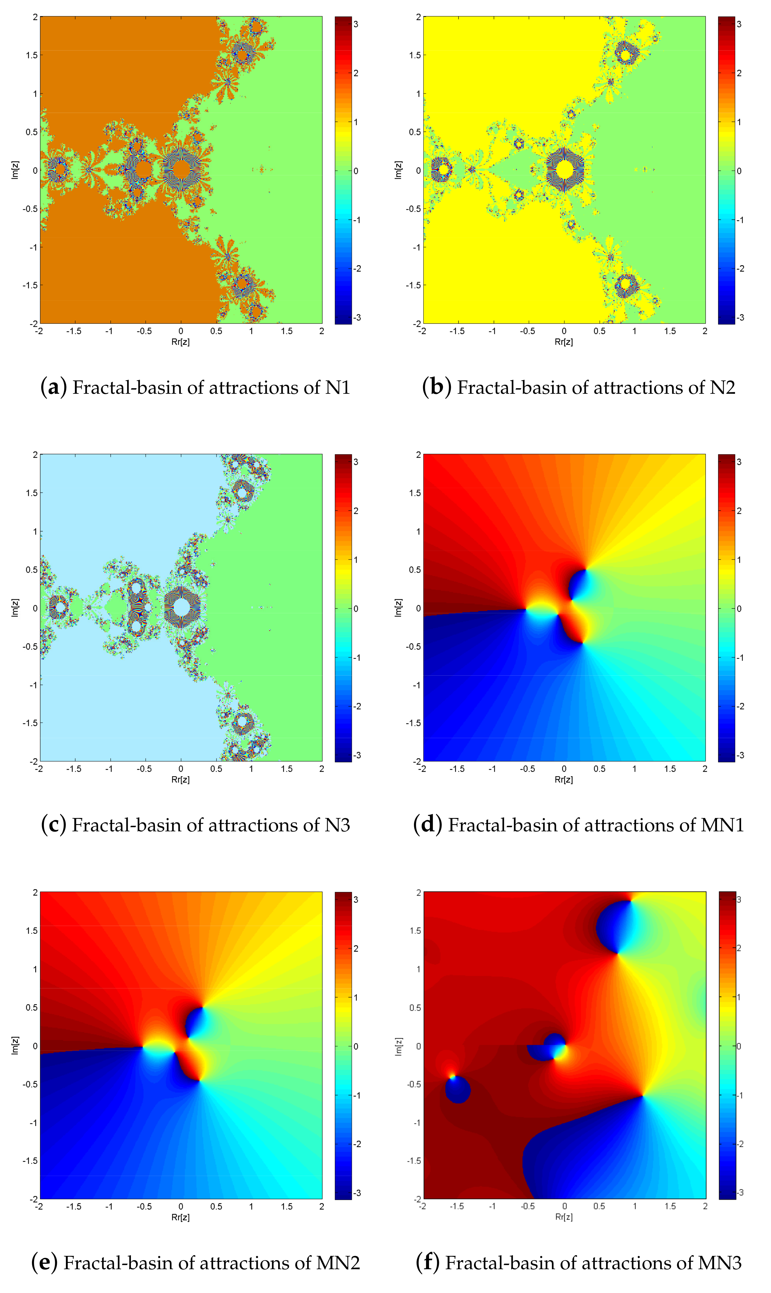
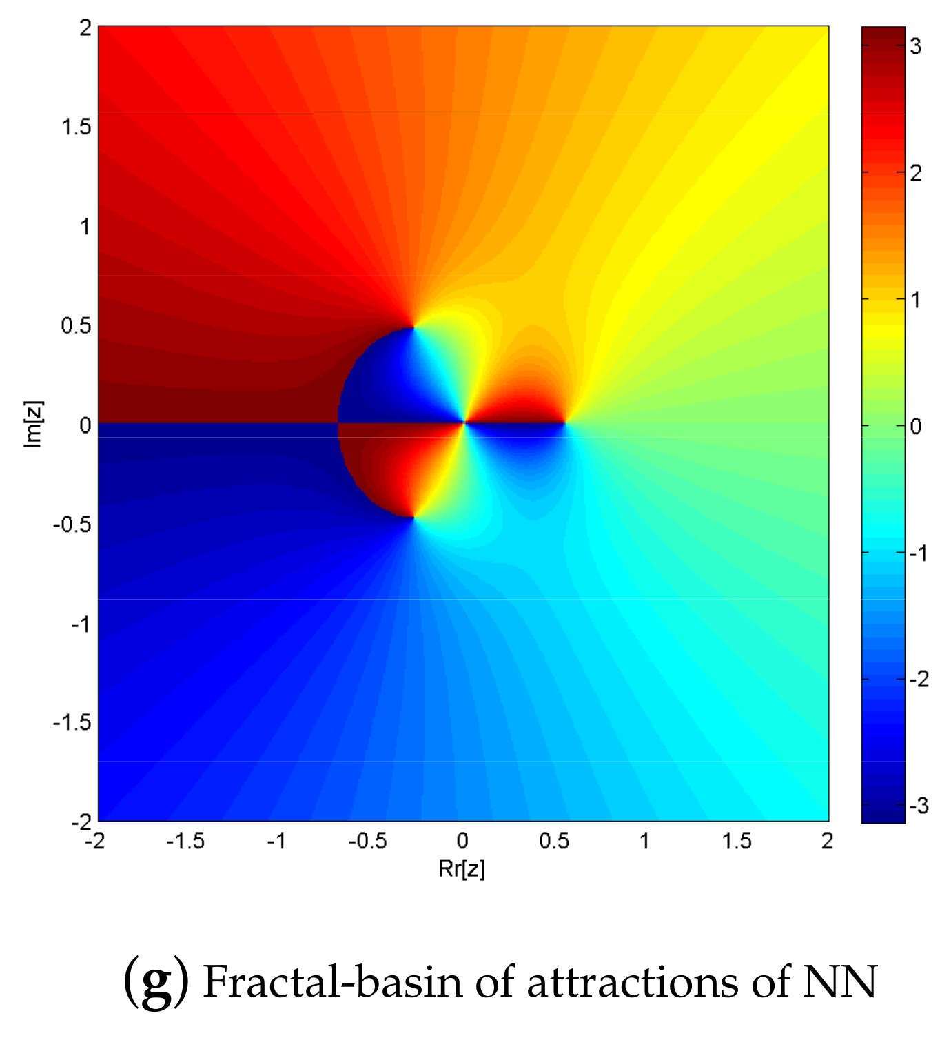
Fractal Analysis of Simultaneous Scheme: To provoke the fractal-basin of attractions of iterative schemes N1–N3, MN₁–MN₃, and NN for the determining the roots of nonlinear equation, we execute the real and imaginary parts of the starting approximations represented as two axes over a mesh of $250\times 250$ in complex plane. Use $\left|{\varsigma }^{(\vartheta +1)}-{\varsigma }^{\left(\vartheta \right)}\right|<{10}^{-3}$ as a stopping criteria and consider maximum 3 iterations. We allow different colors to mark to which root the iterative scheme converges and black in other cases. Color brightness in basins shows less number of iterations. Figure 1a–g and Figure 2a–g illustrate the fractal behavior of N₁–N₃, MN₁–MN₃ and NN for fractional-order nonlinear polynomials.

Figure 1a–g, shows basins of attraction for nonlinear function $f\left(\varsigma \right)={\varsigma }^{312/99}-\frac{1}{3}$ of iterative methods N1–N3, MN₁–MN₃, and NN, respectively.

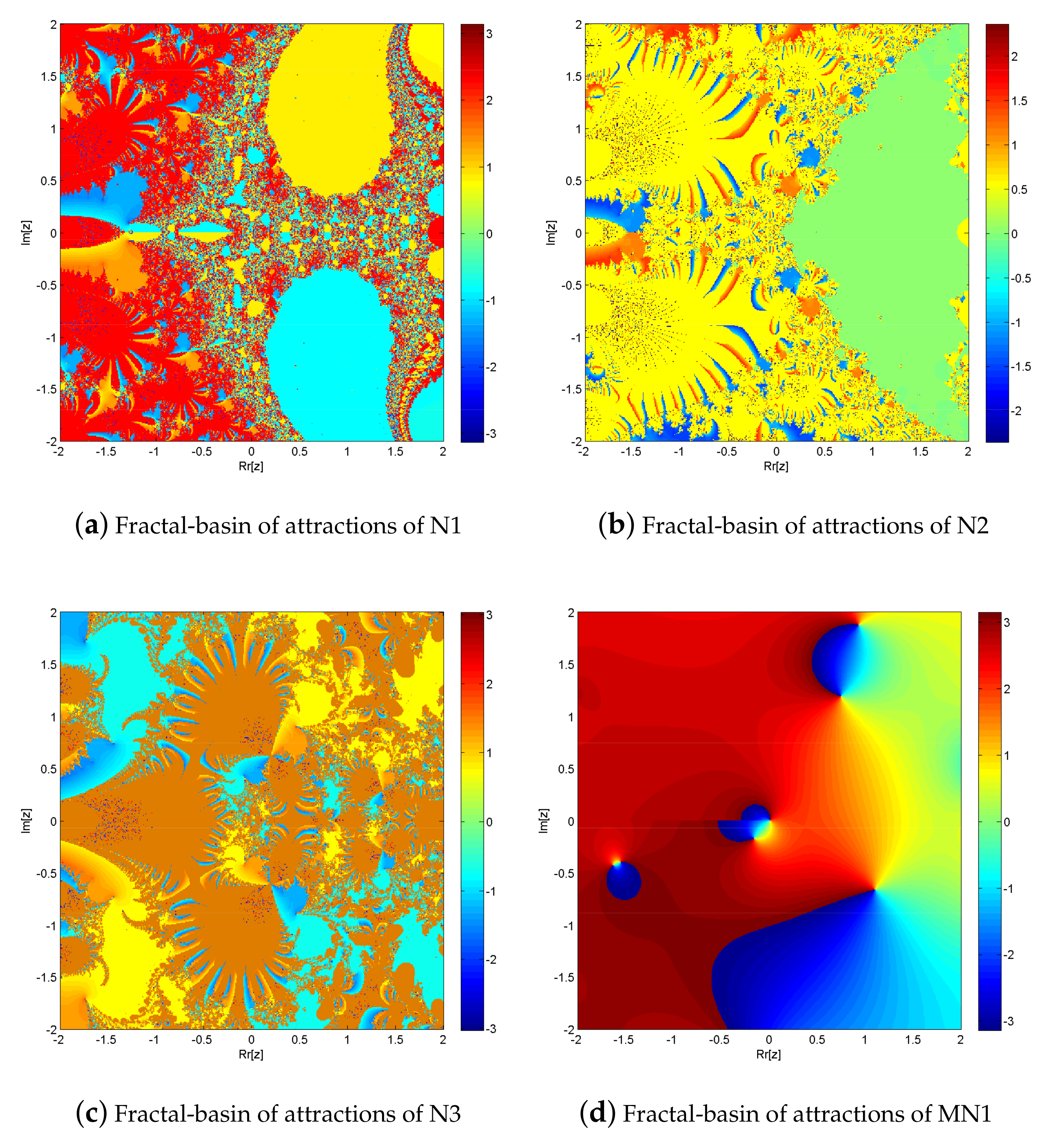
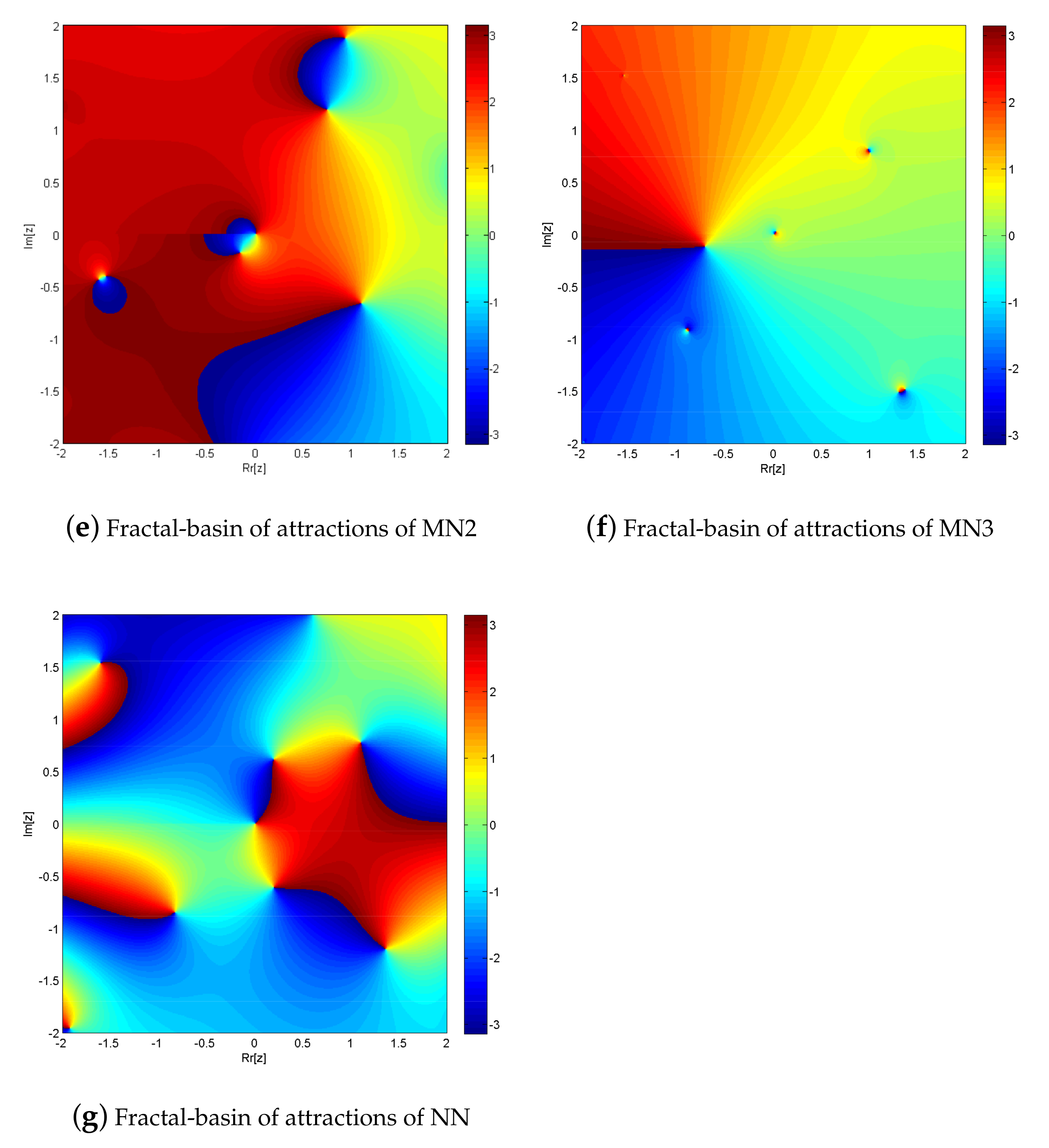
Figure 2a–g, shows basins of attraction for nonlinear function $f\left(\varsigma \right)=e^{{\varsigma }^{210/99}}-log\left(\varsigma \right)$ of iterative methods N1–N3, MN₁–MN₃, and NN, respectively.

From the elapsed time in

Table 1. Elasped time in seconds.

Method	N1	N2	N3	MN1	MN2	MN3	NN
$f\left(\varsigma \right)={\varsigma }^{312/99}-\frac{1}{3}$	5.1293	6.1422	4.3231	0.0714	0.0152	0.0142	0.1235
$f\left(\varsigma \right)=e^{{\varsigma }^{210/99}}-log\left(\varsigma \right)$	4.1609	5.2382	3.4319	0.0124	0.0193	0.0147	0.2145

and brightness in color in Figure 1a–g and Figure 2a–g, shows the dominance behavior of MN₁–MN₃ over N1–N3 and NN, respectively.

The iterative schemes N1–N3, MN₁–MN₃, and NN for solving $f\left(\varsigma \right)={\varsigma }^{312/99}-\frac{1}{3}$, $f\left(\varsigma \right)=e^{{\varsigma }^{210/99}}-log\left(\varsigma \right)$, exhibit fractal behavior, as seen in Figure 1a–g and Figure 2a–g, respectively. In comparison to solving fractional order nonlinear equations $f\left(\varsigma \right)={\varsigma }^{312/99}-\frac{1}{3}$ with N1–N3, MN₁–MN₃, and NN converge to 510,003, 534,673, 507,432, 618,654, 638,765, 632,154, and 588,975 points out of a total of 640,000, respectively. While generating the fractal of $f\left(\varsigma \right)=e^{{\varsigma }^{210/99}}-log\left(\varsigma \right)$, with N1–N3, MN₁–MN₃, and NN converge to 543,254, 543,565, 546,754, 632,455, 63,765, 638,765, and 523,451 points out of a total of 640,000, respectively. Furthermore, MN₁–MN₃ has a far higher convergence rate than NN. In the complex plane, MN₁–MN₃ converges to more points than NN due to global convergence.

3. Computational Aspect

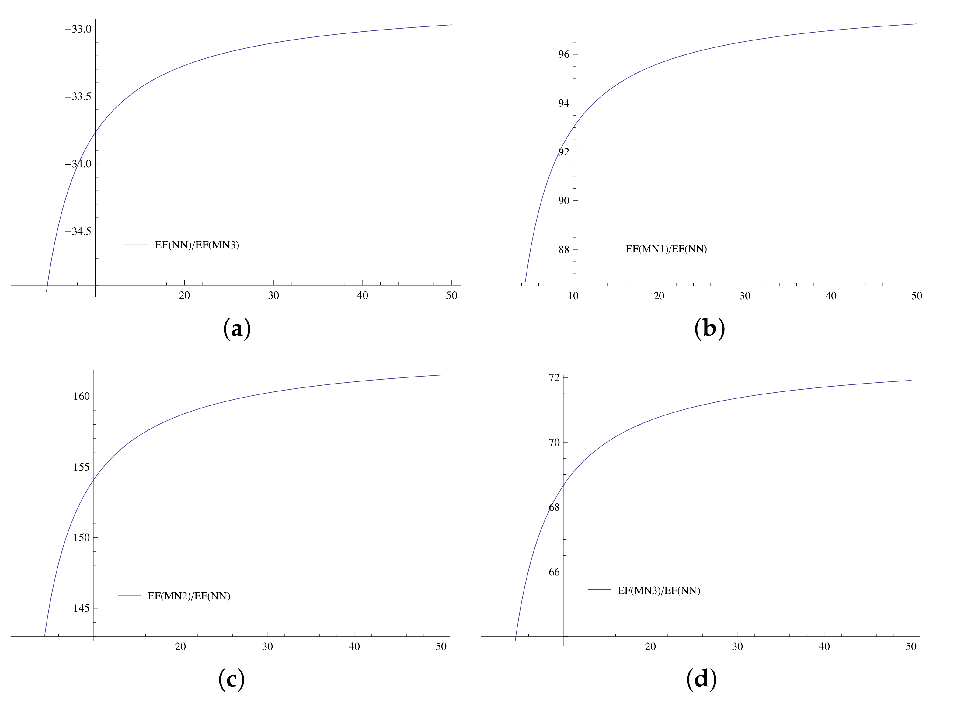
We compare the percentage cost of computation of Midrog Petkovic method (NN-method) [45] and the new family of methods MN₁–MN₃, the computation efficiencies (CE) are computed as:

$$CE\left(m\right)=\frac{\log \mathbf{u}}{\mathbf{D}},$$

(33)

where $\mathbf{D}$ and $\mathbf{u}$ are cost of computation order of convergence of MN₁–MN₃,NN, respectively. Applying (33) and data given in

Table 2. Basic operations per iterations.

	MN1	MN2	MN3	NN
Addition and subtraction	$6⅁$	$7⅁$	$9⅁$	$8⅁$
Multiplications	$1⅁$	$1⅁$	$1⅁$	$6⅁$
Divisions	$2⅁$	$1⅁$	$2⅁$	$2⅁$

where $⅁={⅁}_1+{⅁}_2;{⅁}_1={\mathfrak{m}}^2;{⅁}_2$ = $\mathrm{O}\left(\mathfrak{m}\right).$

, we calculate the percentage computational cost as $\rho ($MN₁–MN₂, NN) [56] given by:

$$\rho (M{N}_1–M{N}_3,\mathrm{NN})=\left(\frac{CE({\mathrm{MN}}_1–{\mathrm{MN}}_3)}{CE\left(\mathrm{NN}\right)}-1\right)\times 100.$$

(34)

Figure 3a–d graphically clarifies these percentage costs of computation. It is obvious from Figure 3b–d, that MN₁–MN₃ are more efficient as compared to NN.

4. Numerical Results

We use CAS Maple 18 with 64-Digits-Floating-Point arithmetic for all numerical calculations with stopping criteria as follows:

$$e_i^{\left(\vartheta \right)}={∥{\varsigma }_i^{\left(\vartheta +1\right)}-{\rho }_i∥}_2<\in ={10}^{-30},$$

where ${\mathrm{e}}_{\mathrm{i}}^{\left(\mathrm{\vartheta }\right)}$ represents the absolute error of norm-2. In all numerical calculations we take $\alpha =0.008,\beta =-0.001,\gamma =1.5.$

Numerical tests problems from [57,58,59,60] are provided in

Table 3. Parallel numerical scheme residual error comparison NN, MN₁–MN₃.

Method	CPU-Time	${\mathrm{e}}_1^{\left(2\right)}$	${\mathrm{e}}_2^{\left(2\right)}$	${\mathrm{e}}_3^{\left(2\right)}$	${\mathrm{e}}_4^{\left(2\right)}$	${\mathrm{e}}_5^{\left(2\right)}$	${\mathrm{e}}_6^{\left(2\right)}$	${\mathrm{e}}_7^{\left(2\right)}$	${\mathrm{e}}_8^{\left(2\right)}$	${\mathrm{e}}_9^{\left(2\right)}$
NN	0.406	0.0	0.0	0.0	5.7 $\times {10}^{-17}$	3.2 $\times {10}^{-21}$	0.0	0.0	0.0	0.0
${\mathrm{MN}}_1$	0.016	0.0	0.0	0.0	0.0	0.0	0.0	0.0	0.0	0.0
${\mathrm{MN}}_2$	0.156	0.0	0.0	0.0	0.0	0.0	0.0	0.0	0.0	0.0
${\mathrm{MN}}_3$	0.159	0.0	0.0	0.0	6.0 $\times {10}^{-37}$	0.9 $\times {10}^{-45}$	0.0	0.0	0.0	0.0

,

Table 4. Approximate roots of the $f_2\left(\varsigma \right)$ utilising MN₁–MN₃ up-to 25 decimal places.

Roots	Approximate Roots after Second Iteration Using Simultaneous Methods MN1–MN3
${\varsigma }_1^{\left(2\right)}$	− 59,696.70991140727878983742649 − 17,330.45629984850327806571946 × i
${\varsigma }_2^{\left(2\right)}$	− 59,696.70991140727878983742649 + 17,330.45629984850327806571946 × i
${\varsigma }_3^{\left(2\right)}$	− 35,422.49261941473703632706384 − 41,931.87069228758403349587288 × i
${\varsigma }_4^{\left(2\right)}$	− 35,422.49261941473703632706384 + 41,931.87069228758403349587288 × i
${\varsigma }_5^{\left(2\right)}$	− 1235.689293801075002171094064 − 42,268.27946411286842679890715 × i
${\varsigma }_6^{\left(2\right)}$	− 1235.689293801075002171094064 + 42,268.27946411286842679890715 × i
${\varsigma }_7^{\left(2\right)}$	10,470.78502392132516903681496 + 0 × i
${\varsigma }_8^{\left(2\right)}$	22,153.98207243945655027389363 − 18,201.65072991473532250086939 × i
${\varsigma }_9^{\left(2\right)}$	22,153.98207243945655027389363 + 18,201.65072991473532250086939 × i

,

Table 5. Parallel numerical scheme residual error comparison NN, MN₁–MN₃.

Method	CPU-Time	${\mathrm{e}}_1^{\left(2\right)}$	${\mathrm{e}}_2^{\left(2\right)}$	${\mathrm{e}}_3^{\left(2\right)}$	${\mathrm{e}}_4^{\left(2\right)}$	${\mathrm{e}}_5^{\left(2\right)}$	${\mathrm{e}}_6^{\left(2\right)}$	${\mathrm{e}}_7^{\left(2\right)}$
NN	4.547	0.1 $\times {10}^{-11}$	3.6 $\times {10}^{-12}$	3.9 $\times {10}^{-10}$	3.3 $\times {10}^{-12}$	1.0 $\times {10}^{-10}$	3.0 $\times {10}^{-11}$	3.0 $\times {10}^{-11}$
${\mathrm{MN}}_1$	1.547	1.1 $\times {10}^{-114}$	3.2 $\times {10}^{-85}$	3.3 $\times {10}^{-113}$	3.6 $\times {10}^{-114}$	3.0 $\times {10}^{-110}$	3.6 $\times {10}^{-98}$	0.0
${\mathrm{MN}}_2$	1.320	1.3 $\times {10}^{-224}$	1.0 $\times {10}^{-115}$	3.0 $\times {10}^{-114}$	1.6 $\times {10}^{-118}$	0.1 $\times {10}^{-117}$	6.9 $\times {10}^{-115}$	0.0
${\mathrm{MN}}_3$	1.016	1.0 $\times {10}^{-214}$	3.0 $\times {10}^{-115}$	1.0 $\times {10}^{-123}$	3.5 $\times {10}^{-117}$	3.0 $\times {10}^{-114}$	2.0 $\times {10}^{-101}$	0.0
Residual errors for finding of all multiple roots of polynomial of degree 10200 with 21 multiple roots
NN	41.406	3.0 $\times {10}^{-3}$	3.6 $\times {10}^{-3}$	1.0 $\times {10}^{-9}$	3.0 $\times {10}^{-3}$	3.1 $\times {10}^{-2}$	2.0 $\times {10}^{-3}$	4.8 $\times {10}^{-7}$
${\mathrm{MN}}_1$	12.510	5.5 $\times {10}^{-18511}$	3.7 $\times {10}^{-3661}$	3.0 $\times {10}^{-3224}$	3.0 $\times {10}^{-1192}$	2.0 $\times {10}^{-498}$	1.1 $\times {10}^{-1518}$	2.5 $\times {10}^{-3866}$
${\mathrm{MN}}_2$	11.320	3.3 $\times {10}^{-17588}$	3.8 $\times {10}^{-2661}$	3.6 $\times {10}^{-3224}$	0.9 $\times {10}^{-1214}$	5.5 $\times {10}^{-385}$	1.0 $\times {10}^{-1517}$	5.0 $\times {10}^{-3513}$
${\mathrm{MN}}_3$	13.033	3.6 $\times {10}^{-14561}$	3.9 $\times {10}^{-4125}$	3.6 $\times {10}^{-3112}$	0.8 $\times {10}^{-2112}$	2.6 $\times {10}^{-396}$	3.6 $\times {10}^{-1311}$	3.6 $\times {10}^{-1501}$
${\mathrm{e}}_8^{\left(2\right)}$	${\mathrm{e}}_9^{\left(2\right)}$	${\mathrm{e}}_{10}^{\left(2\right)}$	${\mathrm{e}}_{11}^{\left(2\right)}$	${\mathrm{e}}_{12}^{\left(2\right)}$	${\mathrm{e}}_{13}^{\left(2\right)}$	${\mathrm{e}}_{14}^{\left(2\right)}$	${\mathrm{e}}_{15}^{\left(2\right)}$	${\mathrm{e}}_{16}^{\left(2\right)}$	${\mathrm{e}}_{17}^{\left(2\right)}$
2.0 $\times {10}^{-12}$	2.3 $\times {10}^{-12}$	1.3 $\times {10}^{-101}$	0.0	0.0	0.0	0.0	0.2 $\times {10}^{-102}$	9.3 $\times {10}^{-90}$	8.9 $\times {10}^{-112}$
0.0	0.0	0.0	0.0	0.0	0.0	0.0	0.0	0.0	9.5 $\times {10}^{-201}$
0.0	0.0	0.0	0.0	0.0	0.0	0.0	0.0	0.0	2.2 $\times {10}^{-121}$
0.0	0.0	0.0	0.0	0.0	0.0	0.0	0.0	0.0	3.1 $\times {10}^{-131}$
using MN1–3, NN
1.0 $\times {10}^{-3}$	3.9 $\times {10}^{-2}$	9.3 $\times {10}^{-1014}$	3.6 $\times {10}^{-3145}$	9.1 $\times {10}^{-1112}$	0.0	0.0	0.0	6.0 $\times {10}^{-1103}$	7.8 $\times {10}^{-330}$
0.0	0.0	9.0 $\times {10}^{-3215}$	4.9 $\times {10}^{-4120}$	7.8 $\times {10}^{-1125}$	0.0	0.0	0.0	0.0	8.2 $\times {10}^{-1205}$
0.0	0.0	5.6 $\times {10}^{-5125}$	0.5 $\times {10}^{-4412}$	8.1 $\times {10}^{-1225}$	0.0	0.0	0.0	0.0	3.6 $\times {10}^{-1225}$
0.0	0.0	1.2 $\times {10}^{-6132}$	5.9 $\times {10}^{-4}$	4.5 $\times {10}^{-4255}$	0.0	0.0	0.0	0.0	4.6 $\times {10}^{-1135}$
${\mathrm{e}}_{18}^{\left(2\right)}$				${\mathrm{e}}_{19}^{\left(2\right)}$		${\mathrm{e}}_{20}^{\left(2\right)}$		${\mathrm{e}}_{21}^{\left(2\right)}$
7.8 $\times {10}^{-91}$				1.0 $\times {10}^{-107}$		9.8 $\times {10}^{-112}$		9.2 $\times {10}^{-111}$
8.7 $\times {10}^{-108}$				3.5 $\times {10}^{-158}$		9.6 $\times {10}^{-319}$		3.2 $\times {10}^{-113}$
1.2 $\times {10}^{-228}$				1.0 $\times {10}^{-118}$		3.2 $\times {10}^{-319}$		1.3 $\times {10}^{-103}$
1.0 $\times {10}^{-128}$				9.0 $\times {10}^{-128}$		1.2 $\times {10}^{-219}$		1.1 $\times {10}^{-123}$
respectively.
6.3 $\times {10}^{-2001}$				3.6 $\times {10}^{-1152}$		6.3 $\times {10}^{-3011}$		3.6 $\times {10}^{-1222}$
0.0				9.8 $\times {10}^{-50122}$		7.2 $\times {10}^{-4513}$		4.5 $\times {10}^{-4135}$
0.0				8.0 $\times {10}^{-50145}$		3.3 $\times {10}^{-4873}$		1.2 $\times {10}^{-4014}$
0.0				9.8 $\times {10}^{-50143}$		0.3 $\times {10}^{-4713}$		3.2 $\times {10}^{-4781}$

,

Table 6. Approximate roots of the $f_3\left(\varsigma \right)$ utilising MN₁–MN₃ up-to 25 decimal places.

Roots	Approximate Roots after Second Iteration Using Simultaneous Methods MN1–MN3
${\varsigma }_1^{\left(2\right)}$	3.9999999999999999999999862205 − 2.534958216275585934291378436 × 10−22 × i
${\varsigma }_2^{\left(2\right)}$	− 0.9999999999999999999999893629 − 5.690633353809298633369220348 × 10−26 × i
${\varsigma }_3^{\left(2\right)}$	1.9999999999999999999989781561 + 2.614467550760436593548580136 × 10−20 × i
${\varsigma }_4^{\left(2\right)}$	− 1.999999999999999999999930336 + 3.160564818685589784758770362 × 10−23 × i
${\varsigma }_5^{\left(2\right)}$	− 2.323214931157996872628855725 × 10−21 + 2.0000000000000000000342 × i
${\varsigma }_6^{\left(2\right)}$	− 2.529298089824518863489277124 × 10−22 − 1.999999999999999999999938556 × i
${\varsigma }_7^{\left(2\right)}$	1.023976376364266788722524957 × 10−21 + 3.000000000000000000005376510 × i
${\varsigma }_8^{\left(2\right)}$	− 2.840865161134075189641229891 × 10−24 − 2.999999999999999999999993380 × i
${\varsigma }_9^{\left(2\right)}$	− 1.0000000000000000000000000011529 + 2.00000000000000000000000000280 × i
${\varsigma }_{10}^{\left(2\right)}$	− 0.99999999999999999999999997808790 − 2.00000000000000000000000105176 × i
${\varsigma }_{11}^{\left(2\right)}$	− 1.0000000000000000000000000003310 + 0.999999999999999999999999960241 × i
${\varsigma }_{12}^{\left(2\right)}$	− 1.00000000000000000000000000005614 − 1.0000000000000000000000001786 × i
${\varsigma }_{13}^{\left(2\right)}$	0.9999999999999999999998888888966375 + 0.99999999999999999999997438242 × i
${\varsigma }_{14}^{\left(2\right)}$	1.00000000000000000000000000004082 − 0.9999999999999999999999999976687 × i
${\varsigma }_{15}^{\left(2\right)}$	2.00000000000000000000000000304411 + 1.000000000000000000000001584937 × i
${\varsigma }_{16}^{\left(2\right)}$	2.00000000000000000000000000050095 − 0.9999999999999999999999999538760 × i
${\varsigma }_{17}^{\left(2\right)}$	1.00000000000000000000000007480959 + 3.000000000000000000000012531548 × i
${\varsigma }_{18}^{\left(2\right)}$	0.999999999999999999999999676240 − 3.000000000000000000000000000014860 × i
${\varsigma }_{19}^{\left(2\right)}$	6.7038343474826752003668885234 × 10−21 + 4.00000000000000000000005924627 × i
${\varsigma }_{20}^{\left(2\right)}$	10.593133679422746292651200009402 − 3.19174226899999915825206220041498 × i
${\varsigma }_{21}^{\left(2\right)}$	1.00000000000000000000000000032127 − 5.51392157952973235574917078 × 10−24 × i

,

Table 7. Parallel numerical scheme residual error comparison NN, MN₁–MN₃.

Method	CPU-Time	${\mathrm{e}}_1^{\left(2\right)}$	${\mathrm{e}}_2^{\left(2\right)}$	${\mathrm{e}}_3^{\left(2\right)}$	${\mathrm{e}}_4^{\left(2\right)}$
NN	0.235	3.1 $\times {10}^{-27}$	0.0	2.1 $\times {10}^{-41}$	0.0
${\mathrm{MN}}_1$	0.201	0.0	0.0	0.0	0.0
${\mathrm{MN}}_2$	0.211	0.0	0.0	0.0	0.0
${\mathrm{MN}}_3$	0.191	0.0	0.0	0.0	0.0
Simultaneous finding of all multiple roots
NN	0.335	1.2 $\times {10}^{-1105}$	0.0	1.2 $\times {10}^{-1613}$	0.0
${\mathrm{MN}}_1$	0.101	7.2 $\times {10}^{-2114}$	1.2 $\times {10}^{-3801}$	1.2 $\times {10}^{-5305}$	5.2 $\times {10}^{-6662}$
${\mathrm{MN}}_2$	0.121	5.2 $\times {10}^{-2100}$	4.2 $\times {10}^{-3710}$	3.2 $\times {10}^{-5211}$	6.2 $\times {10}^{-6653}$
${\mathrm{MN}}_3$	0.311	9.2 $\times {10}^{-2100}$	7.2 $\times {10}^{-3601}$	1.9 $\times {10}^{-5305}$	8.2 $\times {10}^{-6714}$

,

Table 8. Approximate roots of the $f_4\left(\varsigma \right)$ utilising MN₁–MN₃ up-to 25 decimal places.

Roots	Approximate Roots after Second Iteration Using Simultaneous Methods MN1–MN3
${\varsigma }_1^{\left(2\right)}$	0.3000000000000000000000000000 + 0.6000000000000000000000000000 × i
${\varsigma }_2^{\left(2\right)}$	0.1000000000000000000000000000 + 0.7000000000000000000000000000 × i
${\varsigma }_3^{\left(2\right)}$	0.7000000000000000000000000000 + 0.5000000000000000000000000000 × i
${\varsigma }_4^{\left(2\right)}$	0.3000000000000000000000000000 + 0.4000000000000000000000000000 × i

,

Table 9. Parallel numerical scheme residual error comparison NN, MN₁–MN₃.

Method	CPU-Time	${\mathrm{e}}_1^{\left(2\right)}$	${\mathrm{e}}_2^{\left(2\right)}$	${\mathrm{e}}_3^{\left(2\right)}$	${\mathrm{e}}_4^{\left(2\right)}$	${\mathrm{e}}_5^{\left(2\right)}$	${\mathrm{e}}_6^{\left(2\right)}$	${\mathrm{e}}_7^{\left(2\right)}$
NN	0.235	0.3 $\times {10}^{-87}$	3.0 $\times {10}^{-91}$	1.0 $\times {10}^{-90}$	4.3 $\times {10}^{-93}$	5.0 $\times {10}^{-83}$	2.1 $\times {10}^{-12}$	2.1 $\times {10}^{-72}$
${\mathrm{MN}}_1$	0.201	7.3 $\times {10}^{-101}$	3.2 $\times {10}^{-101}$	2.0 $\times {10}^{-110}$	1.3 $\times {10}^{-125}$	3.4 $\times {10}^{-137}$	6.0 $\times {10}^{-112}$	0.3 $\times {10}^{-101}$
${\mathrm{MN}}_2$	0.211	1.7 $\times {10}^{-111}$	0.1 $\times {10}^{-101}$	1.2 $\times {10}^{-101}$	5.5 $\times {10}^{-225}$	7.6 $\times {10}^{-134}$	8.0 $\times {10}^{-112}$	9.3 $\times {10}^{-104}$
${\mathrm{MN}}_3$	0.191	8.3 $\times {10}^{-111}$	9.0 $\times {10}^{-111}$	2.1 $\times {10}^{-101}$	4.3 $\times {10}^{-125}$	3.0 $\times {10}^{-132}$	2.8 $\times {10}^{-112}$	8.3 $\times {10}^{-101}$
	${\mathrm{e}}_8^{\left(2\right)}$	${\mathrm{e}}_9^{\left(2\right)}$	${\mathrm{e}}_{10}^{\left(2\right)}$	${\mathrm{e}}_{11}^{\left(2\right)}$	${\mathrm{e}}_{12}^{\left(2\right)}$	${\mathrm{e}}_{13}^{\left(2\right)}$	${\mathrm{e}}_{14}^{\left(2\right)}$	${\mathrm{e}}_{15}^{\left(2\right)}$
	2.1 $\times {10}^{-82}$	2.5 $\times {10}^{-73}$	9.3 $\times {10}^{-74}$	3.0 $\times {10}^{-77}$	2.1 $\times {10}^{-73}$	1.3 $\times {10}^{-112}$	3.0 $\times {10}^{-98}$	2.0 $\times {10}^{-85}$
	6.1 $\times {10}^{-114}$	7.0 $\times {10}^{-113}$	8.3 $\times {10}^{-115}$	3.5 $\times {10}^{-117}$	2.2 $\times {10}^{-114}$	9.3 $\times {10}^{-117}$	9.0 $\times {10}^{-111}$	2.9 $\times {10}^{-135}$
	3.3 $\times {10}^{-131}$	5.8 $\times {10}^{-101}$	1.5 $\times {10}^{-110}$	3.3 $\times {10}^{-118}$	0.6 $\times {10}^{-115}$	6.3 $\times {10}^{-119}$	0.9 $\times {10}^{-112}$	5.0 $\times {10}^{-131}$
	9.0 $\times {10}^{-120}$	7.6 $\times {10}^{-100}$	7.3 $\times {10}^{-115}$	6.0 $\times {10}^{-120}$	1.7 $\times {10}^{-116}$	7.3 $\times {10}^{-121}$	4.4 $\times {10}^{-115}$	2.5 $\times {10}^{-117}$
${\mathrm{e}}_{16}^{\left(2\right)}$			${\mathrm{e}}_{17}^{\left(2\right)}$			${\mathrm{e}}_{18}^{\left(2\right)}$
1.3 $\times {10}^{-95}$			3.0 $\times {10}^{-95}$			5.0 $\times {10}^{-91}$
2.3 $\times {10}^{-111}$			9.0 $\times {10}^{-102}$			0.1 $\times {10}^{-119}$
1.3 $\times {10}^{-115}$			5.8 $\times {10}^{-113}$			2.9 $\times {10}^{-203}$
5.3 $\times {10}^{-101}$			3.9 $\times {10}^{-114}$			8.0 $\times {10}^{-117}$

,

Table 10. Approximate roots of the $f_5\left(\varsigma \right)$ utilising MN₁–MN₃ up-to 25 decimal places.

Roots	Approximate Roots after Second Iteration Using Simultaneous Methods MN1–MN3
${\varsigma }_1^{\left(2\right)}$	0.8603435385822107751310968108 + 1.854362078138018927197345307 × i
${\varsigma }_2^{\left(2\right)}$	0.8603435385824826826164634926 − 1.854362078137389759121145467 × i
${\varsigma }_3^{\left(2\right)}$	− 0.8603435385824826826191976484 + 1.854362078137389759116467203 × i
${\varsigma }_4^{\left(2\right)}$	− 0.8603435385824826826250491509 − 1.854362078137389758498169291 × i
${\varsigma }_5^{\left(2\right)}$	2.099515617155402337664929826 + 2.0018942089444809594275 × 10−25 × i
${\varsigma }_6^{\left(2\right)}$	− 2.099515617155402337664930488 + 8.500261481816581859095 × 10−65 × i
${\varsigma }_7^{\left(2\right)}$	− 0.1153355754810685747732055498 − 0.9452308584818627592298044050 × i
${\varsigma }_8^{\left(2\right)}$	5.735924944438839111033359624 + 9.9691958921656837672916427681 × i
${\varsigma }_9^{\left(2\right)}$	2.780333195217222311406266628 + 1.5314159752240276458048625411 × i
${\varsigma }_{10}^{\left(2\right)}$	10.38458363502628061602412598 − 2.2689074595992585372659252860 × i
${\varsigma }_{11}^{\left(2\right)}$	− 2.889237782026642801550622077 + 1.387876808887673226733098622 × i
${\varsigma }_{12}^{\left(2\right)}$	− 2.889237274653490024449890492 − 1.387876796309858631439562289 × i
${\varsigma }_{13}^{\left(2\right)}$	2.378876612988062257880708956 + 3.4667457639218525242487229114 × i
${\varsigma }_{14}^{\left(2\right)}$	2.378876612988074253739225478 − 3.4667457639218476882627822682 × i
${\varsigma }_{15}^{\left(2\right)}$	− 2.378876612988074361358332472 + 3.466745763921847828159258028 × i
${\varsigma }_{16}^{\left(2\right)}$	− 2.378876615468194672405838207 − 3.466745742882904234182513076 × i
${\varsigma }_{17}^{\left(2\right)}$	− 1.705508831120901418129885320 × 10−50 + 3.1838193018332206021608 × i
${\varsigma }_{18}^{\left(2\right)}$	2.684827765525257608577503573 × 10−34 − 3.18381930183322060216087 × i

,

Table 11. Parallel numerical scheme residual error comparison NN, MN₁–MN₃.

Method	CPU-Time	${\mathrm{e}}_1^{\left(2\right)}$	${\mathrm{e}}_2^{\left(2\right)}$	${\mathrm{e}}_3^{\left(2\right)}$	${\mathrm{e}}_4^{\left(2\right)}$	${\mathrm{e}}_5^{\left(2\right)}$	${\mathrm{e}}_6^{\left(2\right)}$	${\mathrm{e}}_7^{\left(2\right)}$	${\mathrm{e}}_8^{\left(2\right)}$
NN	3.547	1.0 $\times {10}^{-57}$	3.1 $\times {10}^{-40}$	8.4 $\times {10}^{-51}$	6.6 $\times {10}^{-52}$	1.1 $\times {10}^{-47}$	0.1 $\times {10}^{-51}$	3.1 $\times {10}^{-47}$	0.1 $\times {10}^{-59}$
${\mathrm{MN}}_1$	1.201	0.0	8.4 $\times {10}^{-61}$	8.4 $\times {10}^{-62}$	9.6 $\times {10}^{-62}$	1.6 $\times {10}^{-62}$	0.1 $\times {10}^{-62}$	3.1 $\times {10}^{-63}$	6.1 $\times {10}^{-62}$
${\mathrm{MN}}_2$	2.201	1.5 $\times {10}^{-61}$	5.2 $\times {10}^{-64}$	5.5 $\times {10}^{-61}$	0.9 $\times {10}^{-62}$	0.1 $\times {10}^{-62}$	9.1 $\times {10}^{-62}$	6.1 $\times {10}^{-65}$	7.1 $\times {10}^{-62}$
${\mathrm{MN}}_3$	2.101	0.0	7.1 $\times {10}^{-60}$	54 $\times {10}^{-64}$	0.6 $\times {10}^{-62}$	7.1 $\times {10}^{-62}$	9.1 $\times {10}^{-62}$	3.8 $\times {10}^{-62}$	8.1 $\times {10}^{-62}$
${\mathrm{e}}_9^{\left(2\right)}$				${\mathrm{e}}_{10}^{\left(2\right)}$		${\mathrm{e}}_{11}^{\left(2\right)}$		${\mathrm{e}}_{12}^{\left(2\right)}$
3.5 $\times {10}^{-41}$				4.1 $\times {10}^{-52}$		3.4 $\times {10}^{-57}$		3.7 $\times {10}^{-59}$
9.5 $\times {10}^{-63}$				9.1 $\times {10}^{-61}$		7.7 $\times {10}^{-60}$		0.7 $\times {10}^{-63}$
3.5 $\times {10}^{-65}$				8.1 $\times {10}^{-62}$		3.4 $\times {10}^{-64}$		9.1 $\times {10}^{-61}$
1.0 $\times {10}^{-64}$				4.8 $\times {10}^{-65}$		6.4 $\times {10}^{-67}$		6.7 $\times {10}^{-67}$

,

Table 12. Approximate roots of the $f_6\left(\varsigma \right)$ utilising MN₁–MN₃ up-to 25 decimal places.

Roots	Approximate Roots after Second Iteration Using Simultaneous Methods MN1–MN3.
${\varsigma }_1^{\left(2\right)}$	0.9999999999999625082889225593 + 5.230898364697391997065172835 × 10−13 × i
${\varsigma }_2^{\left(2\right)}$	− 1.000000000000000000437788933 − 6.025279497445305009774428506 × 10−19 × i
${\varsigma }_3^{\left(2\right)}$	4.646633054497955014523803834 × 10−23 − 1.000000000000000000000104279 × i
${\varsigma }_4^{\left(2\right)}$	7.070081680587045867351347555452430 + 1.896634372172127350402444677884 × i
${\varsigma }_5^{\left(2\right)}$	0.707106781188722682564395565555579 + 0.70710678111831121600988084789 × i
${\varsigma }_6^{\left(2\right)}$	0.707106781186547524204653788888888 − 0.707106708811865475234335246205 × i
${\varsigma }_7^{\left(2\right)}$	− 0.707106781186225449342615220000005 + 0.70710678118305664052862413909 × i
${\varsigma }_8^{\left(2\right)}$	− 0.707106781186547522667534642222232 − 0.707106781122865475118767454190 × i
${\varsigma }_9^{\left(2\right)}$	0.3078726620356213541889978222222356 + 2.57715246122258727612850281995 × i
${\varsigma }_{10}^{\left(2\right)}$	0.272083407184584274611022222616488 × 10−1 − 1 + 3.017417711237066199457739396 × i
${\varsigma }_{11}^{\left(2\right)}$	0.999998299931370519781229455555571 + 1.999995421705299555855269774625 × i
${\varsigma }_{12}^{\left(2\right)}$	0.9999999999999999966472269015554873 − 1.999999999999999999407695317157 × i

and

Table 13. Parallel numerical scheme residual error comparison NN, MN₁–MN₃.

Method	CPU-Time	${\mathrm{e}}_1^{\left(2\right)}$	${\mathrm{e}}_2^{\left(2\right)}$	${\mathrm{e}}_3^{\left(2\right)}$	${\mathrm{e}}_4^{\left(2\right)}$	${\mathrm{e}}_5^{\left(2\right)}$	${\mathrm{e}}_6^{\left(2\right)}$	${\mathrm{e}}_7^{\left(2\right)}$	${\mathrm{e}}_8^{\left(2\right)}$
NN	0.506	7.3 $\times {10}^{-42}$	8.1 $\times {10}^{-61}$	4.0 $\times {10}^{-34}$	1.1 $\times {10}^{-35}$	3.0 $\times {10}^{-27}$	4.1 $\times {10}^{-37}$	1.0 $\times {10}^{-31}$	5.0 $\times {10}^{-38}$
${\mathrm{MN}}_1$	0.216	6.0 $\times {10}^{-55}$	9.9 $\times {10}^{-70}$	3.0 $\times {10}^{-42}$	6.1 $\times {10}^{-39}$	2.0 $\times {10}^{-37}$	5.0 $\times {10}^{-38}$	1.2 $\times {10}^{-40}$	5.0 $\times {10}^{-41}$
${\mathrm{MN}}_2$	0.266	5.0 $\times {10}^{-57}$	9.8 $\times {10}^{-72}$	6.0 $\times {10}^{-43}$	8.1 $\times {10}^{-39}$	4.1 $\times {10}^{-38}$	4.1 $\times {10}^{-38}$	5.0 $\times {10}^{-41}$	3.0 $\times {10}^{-42}$
${\mathrm{MN}}_3$	0.259	3.5 $\times {10}^{-58}$	5.0 $\times {10}^{-78}$	4.4 $\times {10}^{-44}$	1.9 $\times {10}^{-39}$	0.0 $\times {10}^{-30}$	5.0 $\times {10}^{-37}$	7.0 $\times {10}^{-40}$	4.0 $\times {10}^{-47}$

and Algorithm 1.

Algorithm 1: For simultaneous scheme MN1 to approximate all distinct and multiple root of (1).

$\left[\begin{array}{c}\mathrm{For}\mathrm{the}\mathrm{preliminary}\mathrm{computations}{\varsigma }_i^{\left(0\right)}(ii=1,..,N),\\ \mathrm{tolerance}\in >0\mathrm{and}\mathrm{set}jj=0\mathrm{for}\mathrm{tt}-\mathrm{iterations}\\ \left[\begin{array}{c}\mathrm{Calculate}\left\{\begin{array}{c}{y}_j^{\left(\vartheta \right)}={\varsigma }_j^{\left(\vartheta \right)}-\frac{f\left({\varsigma }_j^{\left(\vartheta \right)}\right)}{f^{\prime }\left({\varsigma }_j^{\left(\vartheta \right)}\right)},{\upsilon }_j^{\left(\vartheta \right)}=\frac{f\left(h_j^{\left(\vartheta \right)}\right)}{f\left({\varsigma }_j^{\left(\vartheta \right)}\right)}.\\ h_i^{\left(\vartheta \right)}=y_i^{\left(\vartheta \right)}-\frac{1}{2}\left(\begin{array}{c}\frac{f\left({\varsigma }_j^{\left(\vartheta \right)}\right)+\beta f\left(y_j^{\left(\vartheta \right)}\right)}{f\left({\varsigma }_j^{\left(\vartheta \right)}\right)+(\beta -2)f\left(y_j^{\left(\vartheta \right)}\right)}\frac{f\left(y_j^{\left(\vartheta \right)}\right)}{f^{\prime }\left({\varsigma }_j^{\left(\vartheta \right)}\right)}+\\ \frac{f\left(y_j^{\left(\vartheta \right)}\right)}{2\left[\frac{f\left(y_j^{\left(\vartheta \right)}\right)-f\left({\varsigma }_j^{\left(\vartheta \right)}\right)}{y_j^{\left(\vartheta \right)}-{\varsigma }_j^{\left(\vartheta \right)}}\right]-f^{\prime }\left({\varsigma }_j^{\left(\vartheta \right)}\right)}\end{array}\right),\\ w_{1j}=h_j^{\left(\vartheta \right)}-\left(\begin{array}{c}1+\frac{f\left(h_j^{\left(\vartheta \right)}\right)}{f\left({\varsigma }_j^{\left(\vartheta \right)}\right)}\\ +\alpha {\left(\frac{f\left(h_j^{\left(\vartheta \right)}\right)}{f\left({\varsigma }_j^{\left(\vartheta \right)}\right)}\right)}^2\end{array}\right)\left(\frac{f\left(h_j^{\left(\vartheta \right)}\right)}{\begin{array}{c}f[{\varsigma }_j^{\left(\vartheta \right)},h_j^{\left(\vartheta \right)}]-\\ f[{\varsigma }_j^{\left(\vartheta \right)},y_j^{\left(\vartheta \right)},h_j^{\left(\vartheta \right)}]*\\ ({\varsigma }_j^{\left(\vartheta \right)}-h_j^{\left(\vartheta \right)})\end{array}}\right),\\ z_{1j}^{\left(\vartheta \right)}=w_{1j}^{\left(\vartheta \right)}-\frac{f\left(w_j^{\left(\vartheta \right)}\right)}{f[{\varsigma }_j^{\left(\vartheta \right)},w_j^{\left(\vartheta \right)}]+\left(\begin{array}{c}f[y_j^{\left(\vartheta \right)},{\varsigma }_j^{\left(\vartheta \right)},y_j^{\left(\vartheta \right)}]-\\ f[y_j^{\left(\vartheta \right)},{\varsigma }_j^{\left(\vartheta \right)},w_j^{\left(\vartheta \right)}]-\\ f[h_j^{\left(\vartheta \right)},{\varsigma }_j^{\left(\vartheta \right)},w_j^{\left(\vartheta \right)}]\end{array}\right)\left[{\varsigma }_j^{\left(\vartheta \right)}-w_j^{\left(\vartheta \right)}\right]},\end{array}\right.\\ \mathrm{Update}{\varsigma }_i^{(\vartheta +\mathfrak{1})}={\varsigma }_i^{\left(\vartheta \right)}-\frac{{\sigma }_i}{\frac{1}{N\left({\varsigma }_i^{\left(\vartheta \right)}\right)}-{\displaystyle \sum _{\stackrel{\mathfrak{j}=1}{\mathfrak{j}\ne i}}^{\mathfrak{n}}}\left(\frac{{\sigma }_j}{({\varsigma }_i^{\left(\vartheta \right)}-z_{vj}^{\left(\vartheta \right)})}\right)},\\ \mathrm{where}N\left({\varsigma }_i^{\left(\vartheta \right)}\right)=\left(\frac{f\left({\varsigma }_i^{\left(\vartheta \right)}\right)}{f^{\prime }\left({\varsigma }_i^{\left(\vartheta \right)}\right)}\right).\\ {\varsigma }_i^{(\vartheta +\mathfrak{1})}={\varsigma }_i^{\left(\vartheta \right)}(ii=1,\dots ,n).\\ \mathrm{if}{e}_i^{\left(\vartheta \right)}=\left|\left({\varsigma }_i^{(\vartheta +\mathfrak{1})}-{\varsigma }_i^{\left(\vartheta \right)}\right)\right|<\in ={10}^{-30}\mathrm{or}\sigma >tt,\mathrm{then}\mathrm{break}.\end{array}\right.\\ \mathrm{Set}jj=jj+1\mathrm{and}\mathrm{go}\mathrm{to}{1}^{st}-\mathrm{iteration}.\\ \mathrm{End}\mathrm{do}.\end{array}\right.$

Here, we solve some standard nonlinear polynomials arising in biomedical engineering application.

Application in Bio-engineering

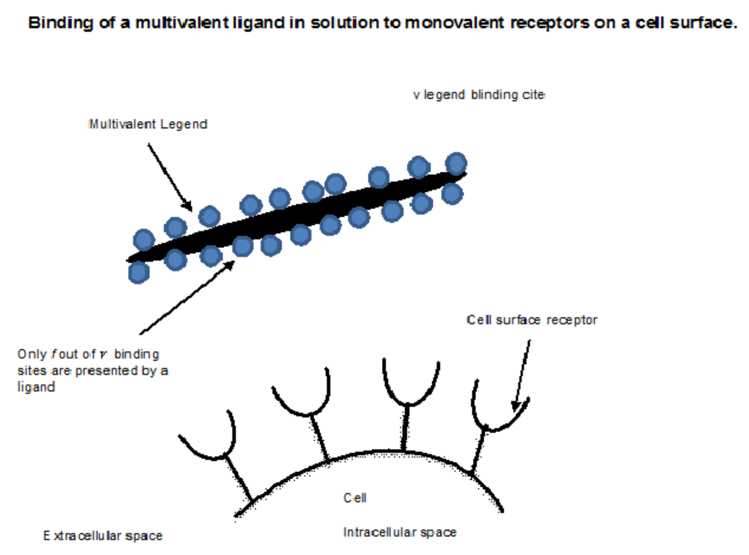
Example 1: Large molecules known as ligands bind to cell surface receptors. Similar to digestive enzymes, sensors are specialized proteins with unique binding attributes that often perform a job when specific ligands are bound, such as transferring a ligand across a cell membrane or activating a signal to turn on specific genes. The process where a ligand can attach to many receptors at once because it has multiple binding sites is referred to as “cross-linking” or “aggregating” numerous receptors. Hormones, antibody–antigen complexes, and other extracellular signaling molecules act as ligands, causing receptors on the cell surface to congregate. For the equilibrium binding of multivalent ligands to cell surface receptors, Perelson [57] presented a model. In this concept, the multivalent ligand is presumed to be available at v active sites for binding to receptors on the surfaces of suspended cells. By coupling one of its v binding sites to a receptor on the cell surface, a ligand molecule can bind to the surface of a cell in solution (see Figure 4). The orientation of the ligand, however, may be able to restrict the variety of binding sites that can interact with a cell once a single link has been created between the ligand and the cell receptor. A ligand may provide f total binding locations for adhering to a cell surface. a ligand’s potential to attach to receptors on the cell surface that have multiple identical binding regions.

The concentration of unbound receptors on the cell surface at equilibrium can be calculated using the following equation:

$$R{R}_T=R{R}_{eq}\left[1+\mathbf{v}\left(\frac{L{L}_0}{K{K}_0}\right){\left(1+K{K}_{\varsigma }R{R}_{eq}\right)}^{\mathbf{f}-1}\right],$$

where

v is the sum of all the binding sites on the component’s surface.

The entire number of binding locations that are accustomed to affixing to an individual cell is f,

$K{K}_{\varsigma }$, Equilibrium constant for multifaceted linking (1/(# ligands/cell)),

$L{L}_0$, Amount of agonist in fluid (M),

$K{K}_D$, The ligand-molecule binding in solution to cells dissociation constant in all three directions (M),

$R{R}_{eq}$, the balance quantity of liberated receptors that are on the outside of the cell (# receptors/cell),

$R{R}_T$, the whole amount of receptors on the surface of platelets.

In order to bind blood platelets cells, a plasma protein known as von Willebrand factor [57] engages in multiple receptor-ligand interactions. The following elements for the von Willebrand factor platelet system are projected:

(i)

$\mathbf{v}=18.00$

(ii)

$\mathbf{f}=9.00$

(iii)

$K{K}_0=7.73\times {10}^{-5}M,$

(iv)

$K{K}_{\varsigma }=5.80\times {10}^{-5}$ cell per number of ligands

(v)

$L{L}_0=2.0\times {10}^{-9}M$

(vi)

$R{R}_T=\mathrm{10,688.00}$ number of receptor per cell

By replacing $R_{eq}$ with $\varsigma$ in a platelet, we want to find the equilibrium concentration $R{R}_{eq}$ of unbound or free receptors as:

$$f_1\left(\varsigma \right)=\varsigma \left[1+\mathbf{v}\left(\frac{L{L}_0}{K{K}_0}\right){\left(1+\varsigma K{K}_{\varsigma }\right)}^{\mathbf{f}-1}\right]-R{R}_T=0,$$

Substituting values of $\mathbf{v},\mathbf{f},K{K}_D,K{K}_{\varsigma },L{L}_0,R{R}_T$ in $f_1\left(\varsigma \right)$ and by simplifying we obtain a nonlinear polynomial of degree 9.0 as:

$$f_2\left(\varsigma \right)=\varsigma \left[1+18\left(\frac{2\times {10}^{-9}}{7.73\times {10}^{-5}}\right){\left(1+5.8\times {10}^{-5}\varsigma \right)}^{9-1}\right]-10688=0,$$

or

$$\begin{array}{ccc}\hfill f_2\left(\varsigma \right)& =& 5.964127997\times {10}^{-38}{\varsigma }^9+8.226383444\times {10}^{-33}{\varsigma }^8+4.964196905\times {10}^{-28}{\varsigma }^7+\hfill \\ & & 1.711792037\times {10}^{-23}{\varsigma }^6+3.689206976\times {10}^{-19}{\varsigma }^5+5.088561346\times {10}^{-15}{\varsigma }^4+\hfill \\ & & 4.386690815\times {10}^{-11}{\varsigma }^3+2.160931436\times {10}^{-7}{\varsigma }^2+1.000465718x-10688.\hfill \end{array}$$

we take the following initial Gaussed values:

$$\begin{array}{ccc}\hfill \stackrel{\left(0\right)}{{\varsigma }_1}& =& -69696-17330i,\stackrel{\left(0\right)}{{\varsigma }_2}=-69696+17330i,{\stackrel{\left(0\right)}{\varsigma }}_3=-45422-41931i,\stackrel{\left(0\right)}{{\varsigma }_4}=-45422+41931i,\hfill \\ \hfill \stackrel{\left(0\right)}{{\varsigma }_5}& =& -2235-42268i,\stackrel{\left(0\right)}{{\varsigma }_6}=-2235+42268i,{\stackrel{\left(0\right)}{\varsigma }}_7=10470,\stackrel{\left(0\right)}{{\varsigma }_8}=22153-18201i,\hfill \\ \hfill \stackrel{\left(0\right)}{{\varsigma }_9}& =& 22153+18201i.\hfill \end{array}$$

For the nonlinear nonlinear problem $f_1\left(\varsigma \right)$, the numerical results of the iterative schemes MN₁–MN₃ and NN are shown in Table 3 and Table 4, respectively.

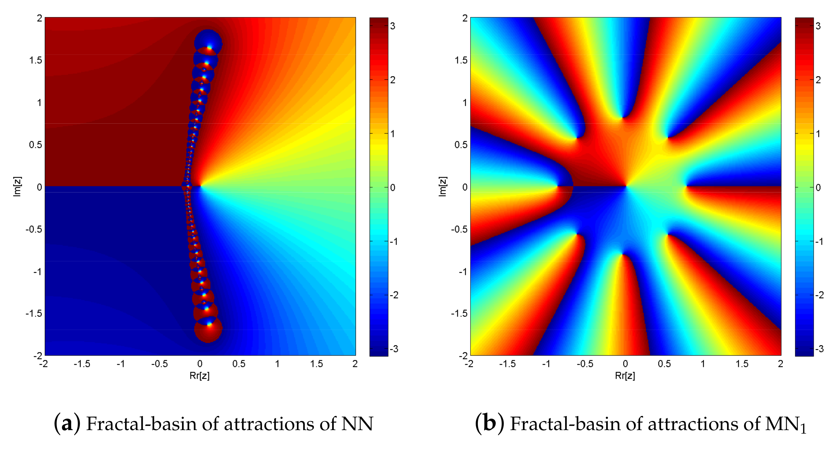
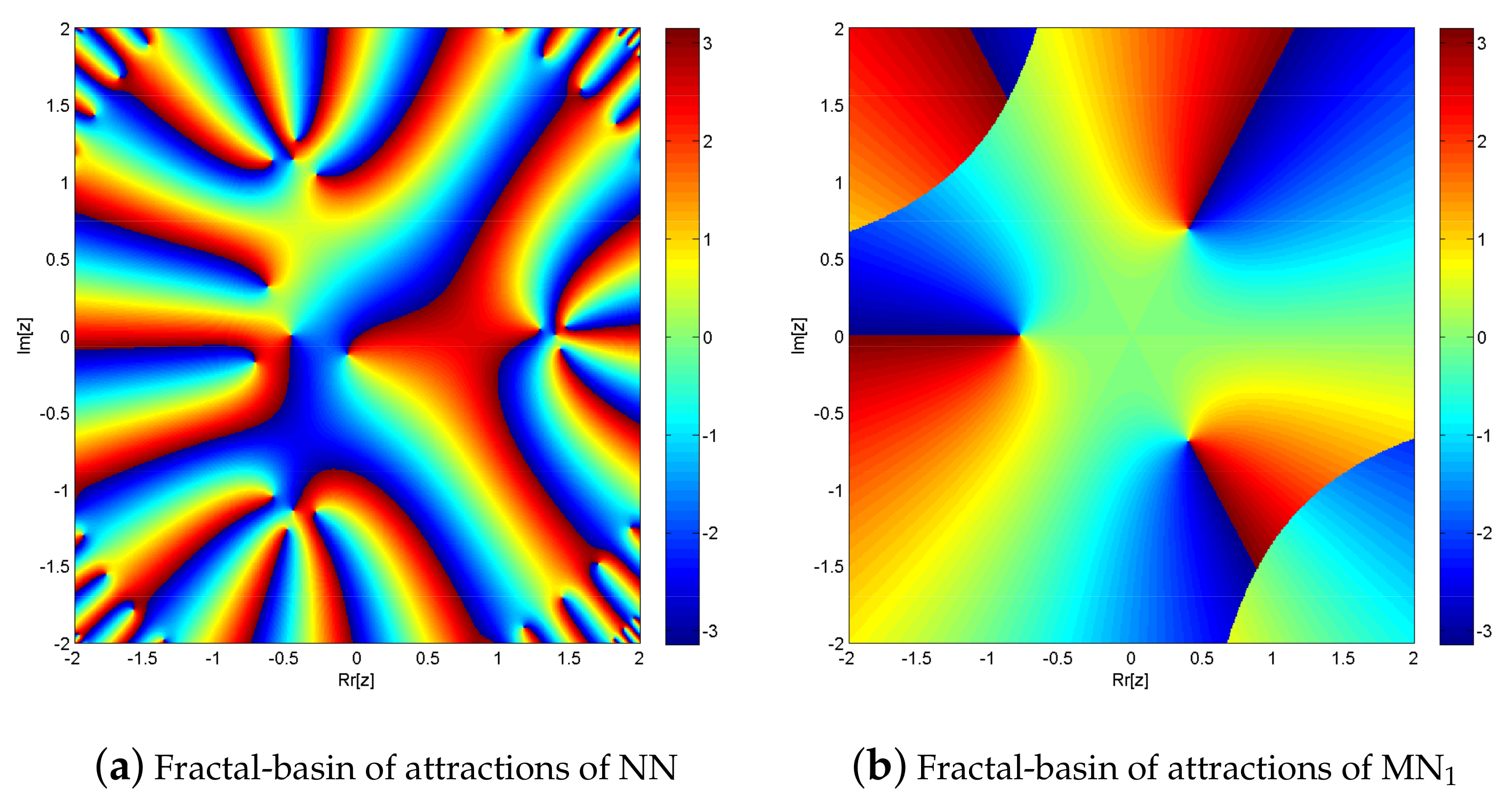
The simultaneous NN and MN₁ for solving $f_2\left(\varsigma \right)$ exhibit fractal behavior, as seen in Figure 5a,b. In comparison to solving fractional order polynomial equations, solving $f_2\left(\varsigma \right)$ with NN and MN₁ takes 0.016774 s and 0.0145 s, respectively. Furthermore, MN₁ has a far higher convergence rate than NN. In the complex plane, NN converges to 512,412 points while MN₁ converges to 631,243 points out of a total of 640,000. Due to global convergence, MN₂ and MN₃ exhibit the same fractal behavior as MN₁.

Example 2: [58] Standard polynomial of degree 10,000 with 21 multiple roots of multiplicities 600, 100, 100, 200, 200, 200, 200, 300, 300, 400, 400, 500, 500, 600, 600, 700, 700, 800, 800, 900, and 900, respectively.

Consider

$$\begin{array}{ccc}\hfill f_3\left(\varsigma \right)& =& {(\varsigma -4)}^{600}{({\varsigma }^2-1)}^{100}{({\varsigma }^4-16)}^{200}{({\varsigma }^2+9)}^{300}{({\varsigma }^2+16)}^{400}{({\varsigma }^2+2\varsigma +5)}^{500}{({\varsigma }^2+2\varsigma +2)}^{600}\hfill \\ & & {({\varsigma }^2-2\varsigma +2)}^{700}{({\varsigma }^2-4\varsigma +5)}^{800}{({\varsigma }^2-2\varsigma +10)}^{900},\hfill \end{array}$$

with exact real and complex roots:

$$\begin{array}{ccc}\hfill {\xi }_1& =& 4,{\xi }_{2,3}=\pm 1,{\xi }_{4,5,6,7}=\pm 2,{\xi }_{8,9}=\pm 3i,{\xi }_{10,11}=\pm 4i,\hfill \\ \hfill {\xi }_{12,13}& =& -1\pm 2i,{\xi }_{14,15}=-1\pm i,{\xi }_{16,17}=1.0\pm i,-{\xi }_{18,19}=2.0\pm 1i,{\xi }_{20,21}=1.0\pm 3.0i.\hfill \end{array}$$

The initial guessed values below were randomly selected for global convergence:

$$\begin{array}{ccc}\hfill \stackrel{\left(0\right)}{{\varsigma }_1}& =& 4.2+0.1i,\stackrel{\left(0\right)}{{\varsigma }_2}=-1.2+0.1i,{\stackrel{\left(0\right)}{\varsigma }}_3=2.2+0.1i,{\stackrel{\left(0\right)}{\varsigma }}_4=-2.2-0.1i,{\stackrel{\left(0\right)}{\varsigma }}_5=0.2+2.1i.\hfill \\ \hfill \stackrel{\left(0\right)}{{\varsigma }_6}& =& 0.2+3.1i,\stackrel{\left(0\right)}{{\varsigma }_7}=0.2-3.1i,{\stackrel{\left(0\right)}{\varsigma }}_8=-1.2+2.1i,{\stackrel{\left(0\right)}{\varsigma }}_9=-1.2-2.1i,{\stackrel{\left(0\right)}{\varsigma }}_{10}=-1.2-2.1i.\hfill \\ \hfill \stackrel{\left(0\right)}{{\varsigma }_{11}}& =& -1.2+1.1i,\stackrel{\left(0\right)}{{\varsigma }_{12}}=-1.2-1.1i,{\stackrel{\left(0\right)}{\varsigma }}_{13}=1.2+1.1i,{\stackrel{\left(0\right)}{\varsigma }}_{14}=1.2-1.1i,{\stackrel{\left(0\right)}{\varsigma }}_{15}=2.2+1.1i.\hfill \\ \hfill \stackrel{\left(0\right)}{{\varsigma }_{16}}& =& 2.2-1.1i,\stackrel{\left(0\right)}{{\varsigma }_{17}}=1.2+3.1i,{\stackrel{\left(0\right)}{\varsigma }}_{18}=1.2-3.1i,{\stackrel{\left(0\right)}{\varsigma }}_{19}=0.2+4.1i,{\stackrel{\left(0\right)}{\varsigma }}_{20}=1.2-4.1i.\hfill \\ \hfill \stackrel{\left(0\right)}{{\varsigma }_{21}}& =& 1.1+0.2i,\hfill \end{array}$$

For distinct roots:

$$\begin{array}{ccc}\hfill f_{3*}\left(\varsigma \right)& =& {(\varsigma -4)}^{600}{({\varsigma }^2-1)}^{100}{({\varsigma }^4-16)}^{200}{({\varsigma }^2+9)}^{300}{({\varsigma }^2+16)}^{400}{({\varsigma }^2+2\varsigma +5)}^{500}{({\varsigma }^2+2\varsigma +2)}^{600}\hfill \\ & & {({\varsigma }^2-2\varsigma +2)}^{700}{({\varsigma }^2-4\varsigma +5)}^{800}{({\varsigma }^2-2\varsigma +10)}^{900}.\hfill \end{array}$$

Table 5 and Table 6, shows numerical results of iterative schemes MN₁–MN₃ and NN for nonlinear equation $f_3\left(\varsigma \right),$$f_{3*}\left(\varsigma \right)$, respectively.

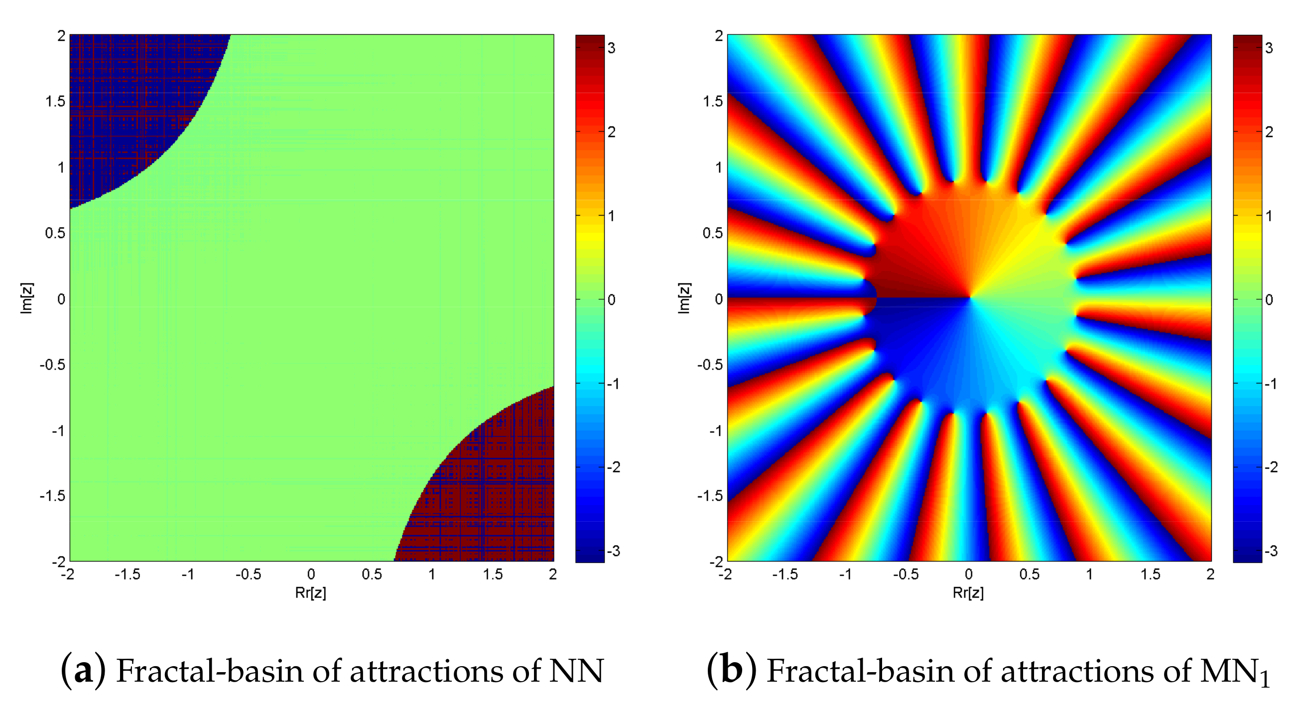
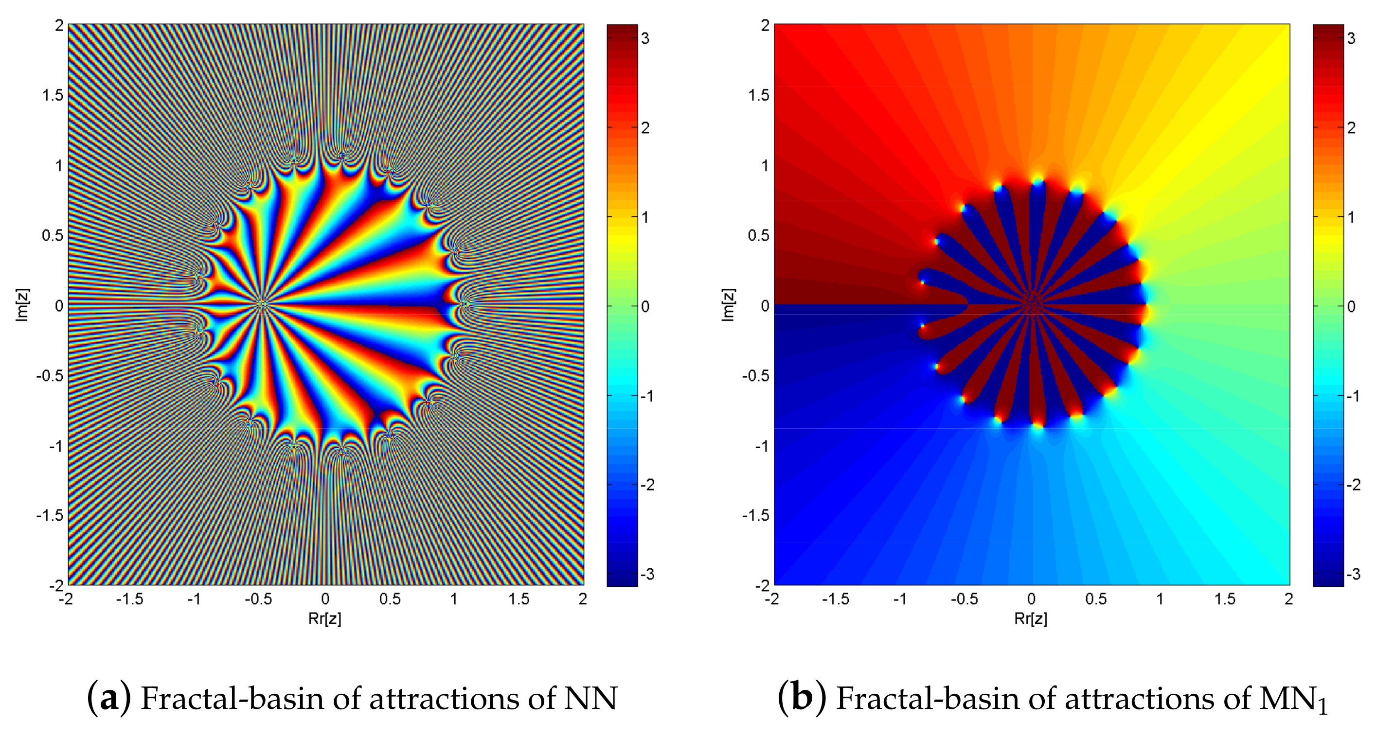
The simultaneous NN and MN₁ for solving $f_3\left(\varsigma \right)$ exhibit fractal behavior, as seen in Figure 6a,b. In comparison to solving fractional order polynomial equations, solving $f_3\left(\varsigma \right)$ with NN and MN₁ takes 0.008774 s and 0.00135 s, respectively. Furthermore, MN₁ has a far higher convergence rate than NN. In the complex plane, NN converges to 212,413 points while MN₁ converges to 621,345 points out of a total of 640,000. Due to global convergence, MN₂ and MN₃ exhibit the same fractal behavior as MN₁.

Example 3: [58] Standard polynomial of degree 1000 with four multiple roots with multiplicities 100, 200, 300, and 400, respectively.

Consider a problem of beam positioning, resulting a nonlinear polynomial equation given as:

$$f_4\left(\varsigma \right)={\left(\varsigma -\left(0.3+0.6i\right)\right)}^{100}{\left(\varsigma -\left(0.1+0.7i\right)\right)}^{200}{\left(\varsigma -\left(0.7+0.5i\right)\right)}^{300}{\left(\varsigma -\left(0.3+0.4i\right)\right)}^{400}.$$

(35)

The exact roots of (35) are ${\xi }_1=0.3+0.6i,$${\xi }_2=0.1+0.7i,$${\xi }_3=0.7+0.5i$,${\xi }_4=0.3+0.4i$.

The initial estimates for $f_4\left(\varsigma \right)$ are:

$$\stackrel{\left(0\right)}{{\varsigma }_1}=0.301+0.601i,\stackrel{\left(0\right)}{{\varsigma }_2}=0.100+0.702i,{\stackrel{\left(0\right)}{\varsigma }}_3=0.702+0.498i,{\stackrel{\left(0\right)}{\varsigma }}_4=0.289+0.400i$$

$$f_{4*}\left(\varsigma \right)=\left(\varsigma -\left(0.3+0.6i\right)\right)\left(\varsigma -\left(0.1+0.7i\right)\right)\left(\varsigma -\left(0.7+0.5i\right)\right)\left(\varsigma -\left(0.3+0.4i\right)\right).$$

Table 7 and Table 8, presents the computational outcomes of MN₁–MN₃ and NN for nonlinear equation $f_4\left(\varsigma \right),$$f_{4*}\left(\varsigma \right)$, respectively.

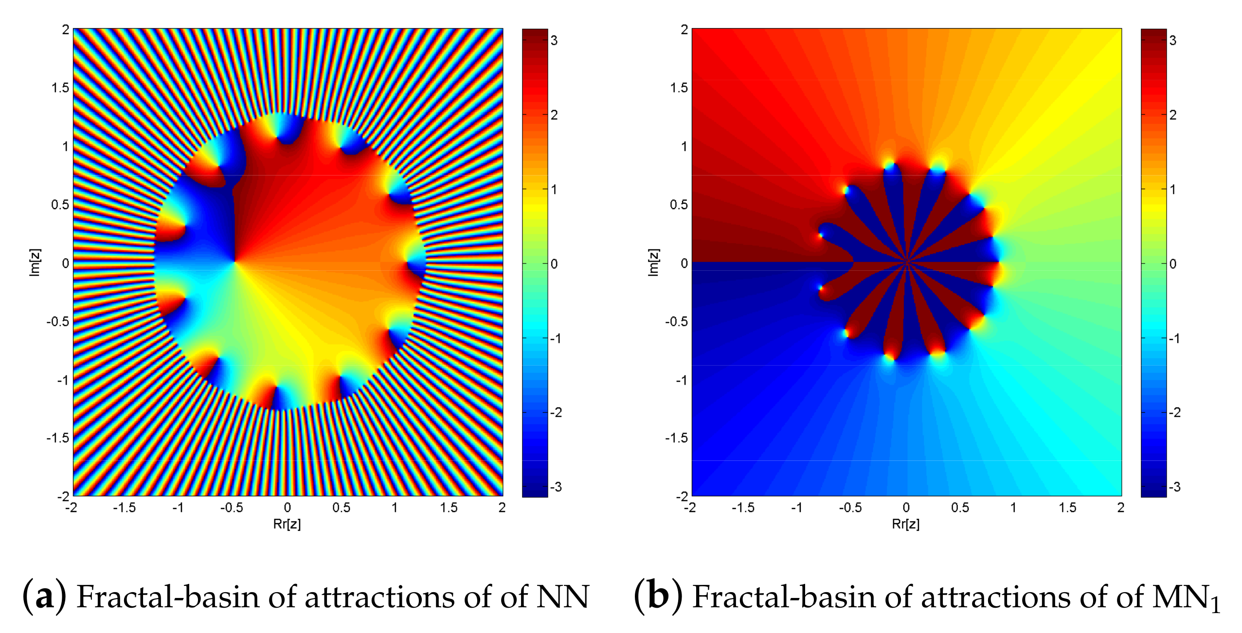
The simultaneous NN and MN₁ for solving $f_4\left(\varsigma \right)$ exhibit fractal behavior, as seen in Figure 7a,b. In comparison to solving fractional order polynomial equations, solving $f_4\left(\varsigma \right)$ with NN and MN₁ takes 0.036774 s and 0.0245 s, respectively. Furthermore, MN₁ has a far higher convergence rate than NN. In the complex plane, NN converges to 610,115 points while MN₁ converges to 637,017 points out of a total of 640,000. Due to global convergence, MN₂ and MN₃ exhibit the same fractal behavior as MN₁.

Example 4: [58] Standard polynomial of degree 18 with four multiple roots.

A nonlinear polynomial equation for a beam alignment problem is as follows:

$$\begin{array}{ccc}\hfill f_5\left(\varsigma \right)& =& {\varsigma }^{18}+12{\varsigma }^{16}+268{\varsigma }^{14}+278{\varsigma }^{12}+3471{\varsigma }^{10}+324696{\varsigma }^8+620972{\varsigma }^6-\hfill \\ & & 2270592{\varsigma }^4-28303951{\varsigma }^2-25704900.\hfill \end{array}$$

(36)

The exact roots of (36) are ${\xi }_{1,2}=-3.06\pm 1.2i,$ ${\xi }_{3,4}=-2.4\pm 3.4i,$ ${\xi }_5=-1.7,{\xi }_{6,7}=-0.6\pm 2.7i$,

${\xi }_{8,9}=\pm 1.8i$, ${\xi }_{10,11}=\pm 0.9i$, ${\xi }_{12,13}=-0.6\pm 2.7i,{\xi }_{14}=1.7,{\xi }_{15,16}=2.4\pm 3.4,{\xi }_{17,18}=3.0\pm 1.2i.$

The initial estimates for $f_5\left(\varsigma \right)$ are:

$$\begin{array}{ccc}\hfill \stackrel{\left(0\right)}{{\varsigma }_1}& =& 1.1+2.1i,\stackrel{\left(0\right)}{{\varsigma }_2}=1.1-2.1i,{\stackrel{\left(0\right)}{\varsigma }}_3=-1.1+2.1i,{\stackrel{\left(0\right)}{\varsigma }}_4=-1.1-2.1i,{\stackrel{\left(0\right)}{\varsigma }}_5=2.2+0.1i.\hfill \\ \hfill \stackrel{\left(0\right)}{{\varsigma }_6}& =& -2.1+0.1i,\stackrel{\left(0\right)}{{\varsigma }_7}=-0.2+0.9i,{\stackrel{\left(0\right)}{\varsigma }}_8=0.2+1.1i,{\stackrel{\left(0\right)}{\varsigma }}_9=3.1+1.9i,{\stackrel{\left(0\right)}{\varsigma }}_{10}=3.2-1.9i.\hfill \\ \hfill \stackrel{\left(0\right)}{{\varsigma }_{11}}& =& -3.2+1.9i,\stackrel{\left(0\right)}{{\varsigma }_{12}}=-3.2-1.9i,{\stackrel{\left(0\right)}{\varsigma }}_{13}=2.1+2.9i,{\stackrel{\left(0\right)}{\varsigma }}_{14}=2.1-2.9i,{\stackrel{\left(0\right)}{\varsigma }}_{15}=-2.1+2.9i.\hfill \\ \hfill \stackrel{\left(0\right)}{{\varsigma }_{16}}& =& -2.1-2.9i,\stackrel{\left(0\right)}{{\varsigma }_{17}}=0.1+3.1i,{\stackrel{\left(0\right)}{\varsigma }}_{18}=-0.1-2.9i.\hfill \end{array}$$

Table 9 and Table 10, shows numerical results of iterative schemes MN₁–MN₃ and NN for nonlinear equation $f_5\left(\varsigma \right)$, respectively.

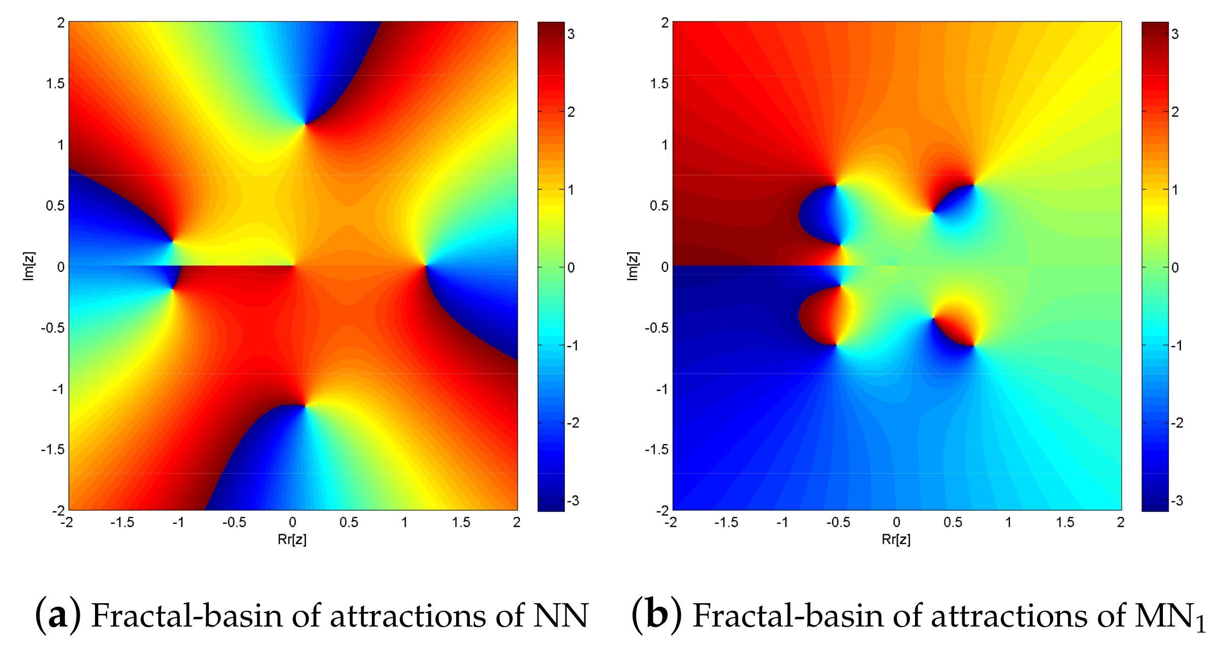
The simultaneous NN and MN₁ for solving $f_5\left(\varsigma \right)$ exhibit fractal behavior, as seen in Figure 8a,b. In comparison to solving fractional order polynomial equations, solving $f_5\left(\varsigma \right)$ with NN and MN₁ takes 0.041294 s and 0.0215445 s, respectively. Furthermore, MN₁ has a far higher convergence rate than NN. In the complex plane, NN converges to 217,615 points while MN₁ converges to 621,971 points out of a total of 640,000. Due to global convergence, MN₂ and MN₃ exhibit the same fractal behavior as MN₁.

Example 5: [58] Standard polynomial of degree 12 with two multiple roots with multiplicity 2 and 8 distinct roots.

Consider the nonlinear polynomial equation:

$$\begin{array}{ccc}\hfill f_6\left(\varsigma \right)& =& {\varsigma }^{12}-(2+5i){\varsigma }^{11}-(1-10i){\varsigma }^{10}+(12-25i){\varsigma }^9-30x^8-{\varsigma }^4+(2+5i){\varsigma }^3+\hfill \\ & & (1-10i){\varsigma }^2-(12-25i)\varsigma +30.\hfill \end{array}$$

(37)

The exact roots of (37) are ${\xi }_{1,2}=\frac{\sqrt{2}}{2}\pm \frac{\sqrt{2}}{2}i,$ ${\xi }_{3,4}=-\frac{\sqrt{2}}{2}\pm \frac{\sqrt{2}}{2}i,$ ${\xi }_{5,6}=1\pm 2i$,

${\xi }_{7,8}=\pm i$, ${\xi }_9=2i,{\xi }_{10}=3i,{\xi }_{11,12}=\pm 1.$

The initial estimates for $f_6\left(\varsigma \right)$ are:

$$\begin{array}{ccc}\hfill \stackrel{\left(0\right)}{{\varsigma }_1}& =& 1.30+0.2i,\stackrel{\left(0\right)}{{\varsigma }_2}=-1.3+0.2i,{\stackrel{\left(0\right)}{\varsigma }}_3=-0.30-1.20i,{\stackrel{\left(0\right)}{\varsigma }}_4=-0.30+1.20i,{\stackrel{\left(0\right)}{\varsigma }}_5=0.5+0.5i,\hfill \\ \hfill \stackrel{\left(0\right)}{{\varsigma }_6}& =& 0.50-0.5i,\stackrel{\left(0\right)}{{\varsigma }_7}=-0.5+0.5i,{\stackrel{\left(0\right)}{\varsigma }}_8=-0.5-0.50i,{\stackrel{\left(0\right)}{\varsigma }}_9=0.2+2.2i,{\stackrel{\left(0\right)}{\varsigma }}_{10}=0.20+2.30i,\hfill \\ \hfill \stackrel{\left(0\right)}{{\varsigma }_{11}}& =& 1.30+2.20i,\stackrel{\left(0\right)}{{\varsigma }_{12}}=1.3-2.20i,\hfill \end{array}$$

Table 11 and Table 12, shows numerical results of iterative schemes MN₁–MN₃ and NN for nonlinear equation $f_6\left(\varsigma \right)$, respectively.

The simultaneous NN and MN₁ for solving $f_6\left(\varsigma \right)$ exhibit fractal behavior, as seen in Figure 9a,b. In comparison to solving fractional order polynomial equations, solving $f_6\left(\varsigma \right)$ with NN and MN₁ takes 0.0745321 s and 0.0349 s, respectively. Furthermore, MN₁ has a far higher convergence rate than NN. In the complex plane, NN converges to 572,416 points while MN₁ converges to 635,097 points out of a total of 640,000. Due to global convergence, MN₂ and MN₃ exhibit the same fractal behavior as MN₁.

Example 6. Model of Blood Rheology [59,60] Blood, a non-Newtonian fluid, is modeled using the Casson Fluid. Based to the Casson fluid model, an elementary fluid, like bloodstream, is going to move through a tube so that the gradient in velocity happens near the wall and the center portion of the fluid goes as a lump with little deformation.

We developed the plug flow of Casson fluids [60] using the following nonlinear polynomial equation, where flow rate reduction is measured by

$$G=1-\frac{16}{7}\sqrt{\varsigma }+\frac{4}{3}\varsigma -\frac{1}{21}{\varsigma }^4,$$

(38)

or where reduction in flow rate is measured by G. Using $G=0.40$ in (38), we have:

$$f_7\left(\varsigma \right)=\frac{1}{441}{\varsigma }^8-\frac{8}{63}{\varsigma }^5-0.05714285714{\varsigma }^4+\frac{16}{9}{\varsigma }^2-3.624489796\varsigma +0.36.$$

(39)

The simultaneous NN and MN₁ for solving $f_7\left(\varsigma \right)$ exhibit fractal behavior, as seen in Figure 10a,b. In comparison to solving fractional order polynomial equations, solving $f_7\left(\varsigma \right)$ with NN and MN₁ takes 0.016774 s and 0.0145 s, respectively. Furthermore, MN₁ has a far higher convergence rate than NN. In the complex plane, NN converges to 630,819 points while MN₁ converges to 639,514 points out of a total of 640,000. Due to global convergence, MN₂ and MN₃ exhibit the same fractal behavior as MN₁.

The exact roots of (38) are:

$$\begin{array}{ccc}\hfill {\zeta }_1& =& 0.1046986515,{\zeta }_2=3.822389235,{\zeta }_3=1.553919850+0.9404149899i,\hfill \\ \hfill {\zeta }_4& =& -1.238769105+3.408523568i,{\zeta }_5=-2.278694688+1.987476450i\hfill \\ \hfill {\zeta }_6& =& -2.278694688-1.987476450i,{\zeta }_7=-1.238769105-3.408523568,\hfill \\ \hfill {\zeta }_8& =& 1.553919850-0.9404149899.\hfill \end{array}$$

we take the following initial guesses:

$$\begin{array}{ccc}\hfill \stackrel{\left(0\right)}{{\varsigma }_1}& =& 0.1,\stackrel{\left(0\right)}{{\varsigma }_2}=3.8,{\stackrel{\left(0\right)}{\varsigma }}_3=1.5+0.9i,{\stackrel{\left(0\right)}{\varsigma }}_4=1.2+3.4i.\hfill \\ \hfill \stackrel{\left(0\right)}{{\varsigma }_5}& =& -2.2+1.9i,\stackrel{\left(0\right)}{{\varsigma }_6}=-2.2-1.9i\stackrel{\left(0\right)}{{\varsigma }_7}=-1.2-3.4i,{\stackrel{\left(0\right)}{\varsigma }}_8=1.5+0.9i.\hfill \end{array}$$

Table 13, shows numerical results of iterative schemes MN₁–MN₃ and NN for nonlinear equation $f_7\left(\varsigma \right)$, respectively.

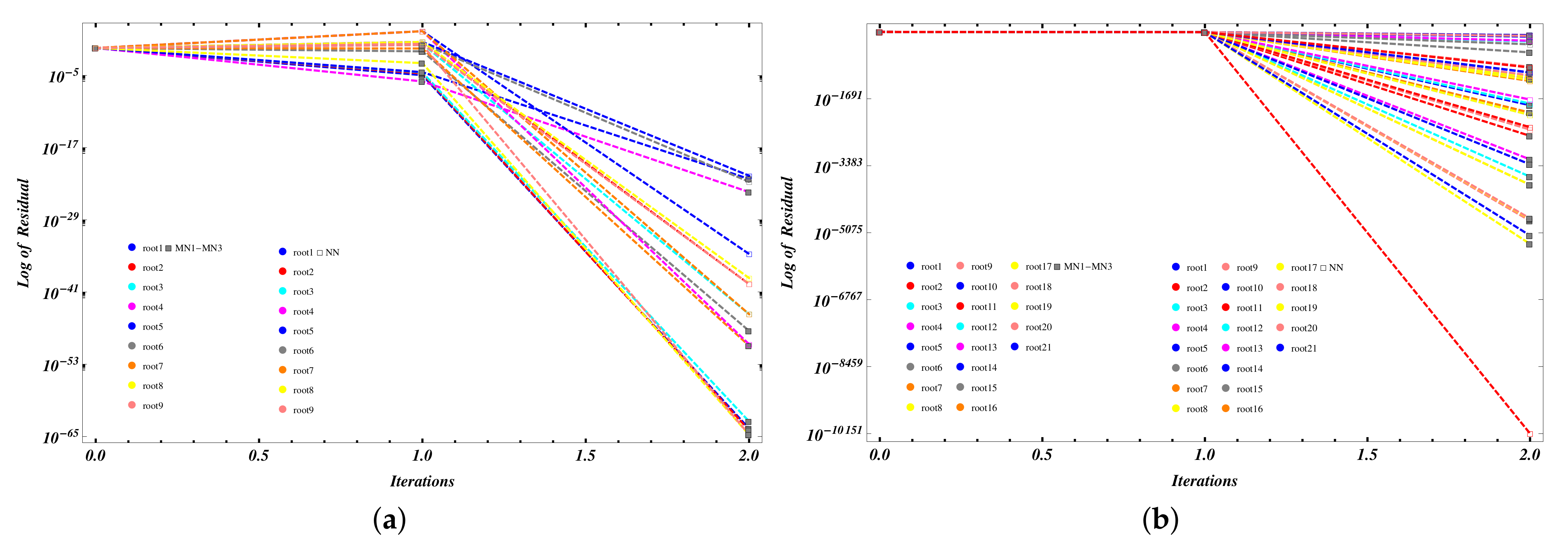
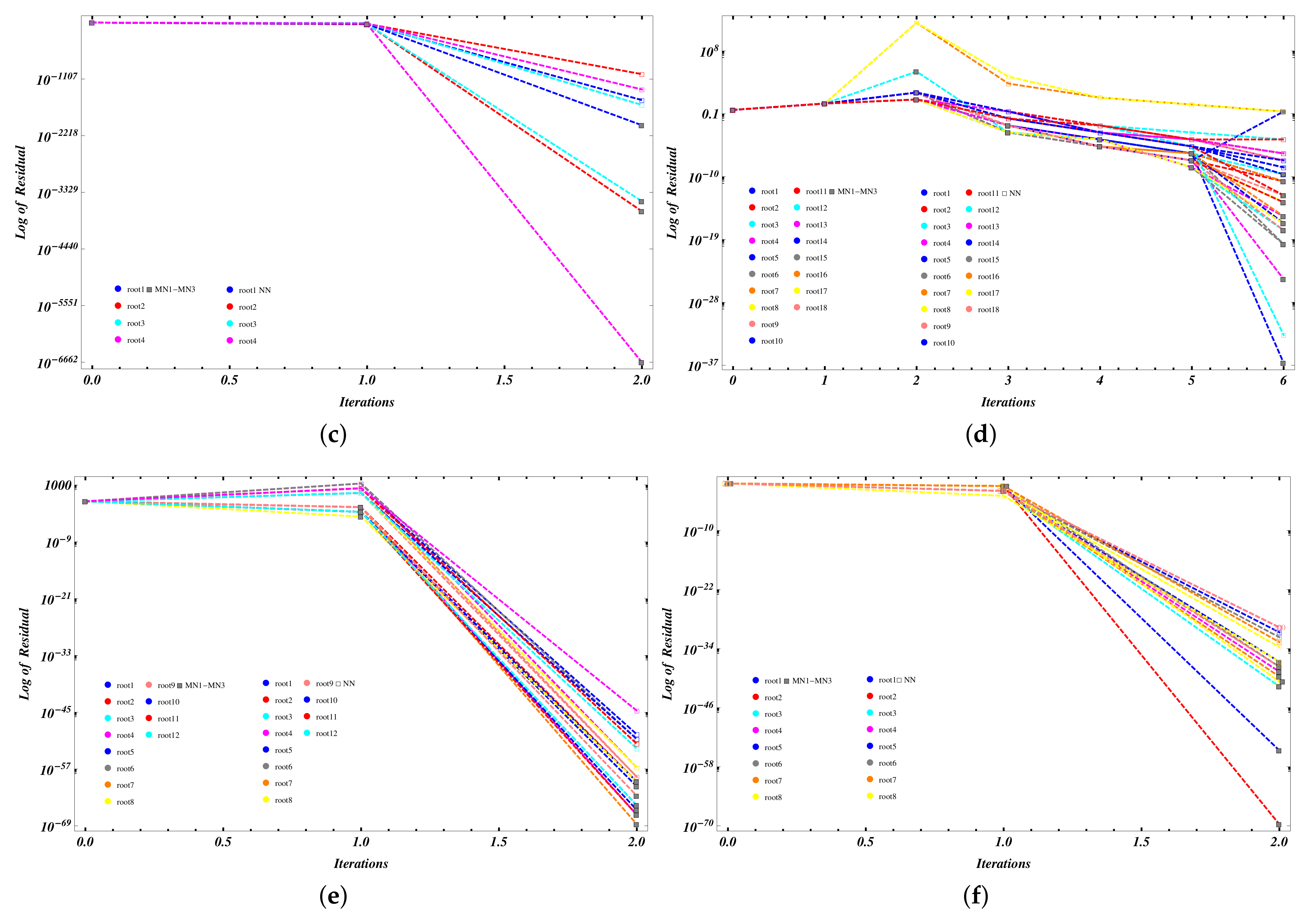
Figure 11a−f, shows the residual error graph of the simultaneous method MN₁–MN₃ and NN for polynomial equations used in examples 1–6, respectively.

5. Conclusions

Here, we have developed three families of simultaneous methods of convergence order seventeenth for finding all the real, complex, distinct, and multiple roots of (1). Fractal behavior from Figure 1, Figure 2, Figure 3, Figure 4, Figure 5, Figure 6, Figure 7, Figure 8, Figure 9 and Figure 10 of simultaneous schemes is explored in detail, and it is discovered that in terms of convergence divergence region, our newly created methods MN₁–MN₃ converge to more points than NN methods while using less elapsed time. The fractal behavior of simultaneous techniques clearly indicated that the newly developed methods are more stable, consistent, and reliable than existing methods N1–N3 and NN for solving nonlinear complex engineering problems. The numerical results from Table 1, Table 2, Table 3, Table 4, Table 5, Table 6, Table 7, Table 8, Table 9, Table 10, Table 11, Table 12 and Table 13, and Figure 11a–f, show that the newly developed technique MN₁–MN₃ outperforms existing method NN in terms of computational cost, efficiency, CPU-time, and residual errors. In the future, we construct higher order efficient, optimal, and stable iterative methods for finding simple as well as all distinct and multiple roots of (1).

In the future, we will develop and generalize higher-order simultaneous methods for solving linear and nonlinear systems of equations. We may also explore the applications of these results in other areas. For example, the dynamics nonlinear inventory management system, numerical solution of fractional SIR epidemiological model, stability and optimal control strategies for a novel epidemic model [61,62] of COVID-19.

References

- Parida, P.K.; Gupta, D.K. An improved method for finding multiple roots and it’s multiplicity of nonlinear equations in R. Appl. Math. Comput. 2008, 202, 498–503. [Google Scholar] [CrossRef]
- Miyakoda, T. Iterative methods for multiple zeros of a polynomial by clustering. J. Comput. Appl. Math. 1989, 28, 315–326. [Google Scholar] [CrossRef]
- Soleymani, F.; Babajee, D.K.R.; Lotfi, T. On a numerical technique for finding multiple zeros and its dynamic. J. Egyp. Math. Soc. 2013, 21, 346–353. [Google Scholar] [CrossRef]
- Traub, J.F. Iterative methods for the solution of equations. Am. Math. Soc. 1982, 312, 1–10. [Google Scholar] [CrossRef]
- Lagouanelle, J.L. Sur une mtode de calcul de l’ordre de multiplicit des zros d’un polynme. C. R. Acad. Sci. Paris Sr. A. 1966, 262, 626–627. [Google Scholar]
- Petković, M.S.; Petković, L.D.; Džunić, J. Accelerating generators of iterative methods for finding multiple roots of nonlinear equations. Comput. Math. Appl. 2010, 59, 2784–2793. [Google Scholar] [CrossRef]
- Johnson, T.; Tucker, W. Enclosing all zeros of an analytic function—A rigorous approach. J. Comput. Appl. Math. 2009, 228, 418–423. [Google Scholar] [CrossRef]
- Fu, D.; Si, Y.; Wang, D.; Xiong, Y. An accelerated neural dynamics model for solving dynamic nonlinear optimization problem and its applications. Chaos Solitons Fractals 2024, 180, 114542. [Google Scholar] [CrossRef]
- Awwal, A.M.; Wang, L.; Kumam, P.; Mohammad, H.; Watthayu, W. A projection Hestenes Stiefel method with spectral parameter for nonlinear monotone equations and signal processing. Math. Comput. Appl. 2020, 25, 27. [Google Scholar] [CrossRef]
- Vyas, S.; Golub, M.D.; Sussillo, D.; Shenoy, K.V. Computation through neural population dynamics. Annu. Rev. Neurosci. 2020, 43, 249–275. [Google Scholar] [CrossRef]
- Ali, K.; Ahmad, A.; Ahmad, S.; Nisar, K.S.; Ahmad, S. Peristaltic pumping of MHD flow through a porous channel: Biomedical engineering application. Waves Random Complex Media 2023, 1, 1–30. [Google Scholar] [CrossRef]
- Ali, H.S.; Habib, M.A.; Miah, M.M.; Akbar, M.A. Solitary wave solutions to some nonlinear fractional evolution equations in mathematical physics. Heliyon 2020, 6, 1–12. [Google Scholar] [CrossRef]
- Chicharro, F.I.; Cordero, A.; Torregrosa, J.R. Drawing dynamical and parameters planes of iterative families and methods. Sci. World J. 2013, 2013, 780153. [Google Scholar] [CrossRef]
- Kung, H.T.; Traub, J.F. Optimal order of one-point and multipoint iteration. J. Assoc. Comput. Mach. 1974, 21, 643–651. [Google Scholar] [CrossRef]
- King, R. Family of fourth-order methods for nonlinear equations. SIAM J. Numer. Anal. 1973, 10, 876–879. [Google Scholar] [CrossRef]
- Cordero, A.; Hueso, J.L.; Martínez, E.; Torregrosa, J.R. New modifications of Potra–Pták’s method with optimal fourth and eighth orders of convergence. J. Comput. Appl. Math. 2010, 234, 2969–2976. [Google Scholar] [CrossRef]
- Chun, C. Fourth-order iterative methods for solving nonlinear equations. Appl. Math. Comput. 2008, 10, 454–459. [Google Scholar] [CrossRef]
- Behl, R.; Kanwar, V.; Sharma, K.K. Modified optimal families of fourth-order Jarratt’s method. Int. J. Pure Appl. Math. 2013, 84, 331–343. [Google Scholar] [CrossRef]
- Kou, J.; Li, Y.; Wang, X. A composite fourth-order iterative method for solving non-linear equations. Appl. Math. Comput. 2007, 184, 471–475. [Google Scholar] [CrossRef]
- Chun, C.; Ham, Y. Some fourth-order modifications of Newton’s method. Appl. Math. Comput. 2008, 197, 654–658. [Google Scholar] [CrossRef]
- Jarratt, P. Some efficient fourth-order multipoint methods for solving equations. BIT 1969, 9, 119–124. [Google Scholar] [CrossRef]
- Chicharro, F.I.; Cordero, A.; Garrido, N.; Torregrosa, J.R. Generating root-finder iterative methods of second order: Convergence and stability. Axioms 2019, 8, 55. [Google Scholar] [CrossRef]
- Ostrowski, A.M. Solution of Equations and Systems of Equations; Prentice-Hall: Englewood Cliffs, NJ, USA, 1964. [Google Scholar]
- Cordero, A.; García-Maimó, J.; Torregrosa, J.R.; Vassileva, M.P.; Vindel, P. Chaos in King’s iterative family. Appl. Math. Lett. 2013, 26, 842–848. [Google Scholar] [CrossRef]
- Weierstrass, K. Neuer Beweis des Satzes, dass jede ganze rationale Function einer Vern derlichen dargestellt werden kann alsein Product aus linearen Functionen derselben Ver n derlichen. Sitzungsberichte K Niglich Preuss. Akad. Der Wiss. Berl. 1981, 2, 1085–1101. [Google Scholar]
- Kerner, I.O. Ein gesamtschrittverfahren zur berechnung der nullstellen von polynomen. Numer. Math. 1966, 8, 290–294. [Google Scholar] [CrossRef]
- Durand, A. Solutions numeriques des equations algebriques Tom 1: Equation du tupe F (I) = 0. Racines d’um Polnome Masson 1960, 2030, 279–281. [Google Scholar]
- Dochev, K. Modified Newton methodfor the simultaneous computation of all roots of a given algebraic equation, in Bulgarian. Phys. Math. J. Bulg. Acad. Sci. 1962, 5, 136–139. [Google Scholar]
- Presic, S. Un proca ditratif pour la factorisation des polynames. C. R. Acad. Sci. Paris 1966, 262, 862–863. [Google Scholar]
- Dochev, K.; Byrnev, P. Certain modifications of Newton’s method for the approximate solution of algebraic equations. USSR Comput. Math. Math. Phy. 1964, 4, 174–182. [Google Scholar] [CrossRef]
- Börsch-Supan, W. Residuenabsch tzung fr Polynom-Nullstellen mittels Lagrange-Interpolation. Numer. Math. 1970, 14, 287–296. [Google Scholar] [CrossRef]
- Ehrlich, L.W. A modified Newton method for polynomials. Commun. ACM 1967, 10, 107–108. [Google Scholar] [CrossRef]
- Nourein, A.W. An improvement on Nourein’s method for the simultaneous determination of the zeroes of a polynomial (an algorithm). J. Comput. Appl. Math. 1977, 3, 109–112. [Google Scholar] [CrossRef]
- Anourein, A.W.M. An improvement on two iteration methods for simultaneous determination of the zeros of a polynomial. Int. J. Comput. Math. 1977, 6, 241–252. [Google Scholar] [CrossRef]
- Sakurai, T.; Torii, T.; Sugiura, H. A high-order iterative formula for simultaneous determination of zeros of a polynomial. J. Comput. Appl. Math. 1991, 38, 387–397. [Google Scholar] [CrossRef]
- Proinov, P.D.; Ivanov, S.I. Convergence analysis of Sakurai-Torii-Sugiura iterative method for simultaneous approximation of polynomial zeros. J. Comput. Appl. Math. 2019, 357, 56–70. [Google Scholar] [CrossRef]
- Proinov, P.; Ivanov, S.I. Local and semi local convergence of an accelerated Sakurai-Torii-Sugiura method with Newton’s correction. In Proceedings of the International Conference of Numerical Analysis and Applied Mathematics, (ICNAAM 2018), Rhodes, Greece, 13–18 September 2018. [Google Scholar]
- Petković, M.S.; Stefanovic, L.V. On some improvements of square root iteration for polynomial complex zeros. J. Comput. Appl. Math. 1986, 15, 13–25. [Google Scholar] [CrossRef]
- Wang, D.R.; Wu, Y.J.; Wang, D. Some modifications of the parallel Halley iteration method and their convergence. Computing 1987, 38, 75–87. [Google Scholar] [CrossRef]
- Petković, M.S.; Triokovic, S.; Herceg, D. On Euler-like methods for the simultaneous approximation of polynomial zeros. Jpn. J. Ind. Appl. Math. 1998, 15, 295–315. [Google Scholar] [CrossRef]
- Proinov, P.D.; Ivanov, S.I.; Petković, M.S. On the convergence of Gander’s type family of iterative methods for simultaneous approximation of polynomial zeros. Appl. Math. Comput. 2019, 349, 168–183. [Google Scholar] [CrossRef]
- Neves Machado, R.; Lopes, L.G. Ehrlich-type methods with King’s correction for the simultaneous approximation of polynomial complex zeros. Math. Stat. 2019, 7, 129–134. [Google Scholar] [CrossRef]
- Proinov, P.D.; Vasileva, M.T. A new family of high-order ehrlich-type iterative methods. Mathematics 2021, 9, 1855. [Google Scholar] [CrossRef]
- Shams, M.; Carpentieri, B. Efficient Inverse Fractional Neural Network-Based Simultaneous Schemes for Nonlinear Engineering Applications. Fractal Fract. 2023, 7, 849. [Google Scholar] [CrossRef]
- Petković, M.S.; Petković, L.D.; Duni, J. On an efficient simultaneous method for finding polynomial zeros. Appl. Math. Lett. 2014, 28, 60–65. [Google Scholar] [CrossRef]
- Proinov, P.D.; Petkova, M.D. Local and semilocal convergence of a family of multi-point Weierstrass-type root finding methods. Mediterr. J. Math. 2020, 17, 107. [Google Scholar] [CrossRef]
- Proinov, P.D.; Vasileva, M.T. On the convergence of high-order Ehrlich-type iterative methods for approximating all zeros of a polynomial simultaneously. J. Ineq. Appl. 2015, 1, 1–25. [Google Scholar] [CrossRef]
- Chinesta, F.; Cordero, A.; Garrido, N.; Torregrosa, J.R.; Triguero-Navarro, P. Simultaneous roots for vectorial problems. Comput. Appl. Math. 2023, 42, 227. [Google Scholar] [CrossRef]
- Cordero, A.; Garrido, N.; Torregrosa, J.R.; Triguero-Navarro, P. An iterative scheme to obtain multiple solutions simultaneously. Appl. Math. Lett. 2023, 145, 108738. [Google Scholar] [CrossRef]
- Shams, M.; Kausar, N.; Araci, S.; Oros, G.I. Numerical scheme for estimating all roots of non-linear equations with applications. AIMS Math. 2023, 8, 23603–23620. [Google Scholar] [CrossRef]
- Aberth, O. Iteration methods for finding all zeros of apolynomial simultaneously. Math. Comp. 1973, 27, 339–344. [Google Scholar] [CrossRef]
- Alefeld, G.; Herzberger, J. Introduction to Interval Computation; Academic Press: Cambridge, MA, USA, 2012. [Google Scholar]
- Milovanovic, G.V.; Petkovic, M.S. On computational efficiency of the iterative methods for the simultaneous approximation ofpolynomial zeros. ACM Trans. Math. Softw. 1986, 12, 295–306. [Google Scholar] [CrossRef]
- Petković, M.S.; Petković, L.D.; Džunić, J. On an efficient method for the simultaneous approximation of polynomial multiple root. Appl. Anal. Discret. Math. 2014, 8, 73–94. [Google Scholar] [CrossRef]
- Rafiq, N. Numerical Solution of Nonlinear Equations; CASPAM, Bahauddin Zakariya University: Multan, Pakistan, 2014. [Google Scholar]
- Mir, N.A.; Shams, M.; Rafiq, N.; Akram, S.; Ahmed, R. On Family of Simultaneous Method for Finding Distinct as Well as MultipleRoots of Non-linear Equation. Punjab Univ. J. Math. 2020, 52, 31–44. [Google Scholar]
- Fournier, R.L. Basic Transport Phenomena in Biomedical Engineering; Taylor & Franics: New York, NY, USA, 2007. [Google Scholar]
- Farmer, M.R. Computing the Zeros of Polynomials Using the Divide and Conquer Approach. Ph.D. Thesis, Department of Computer Science and Information Systems, Birkbeck, University of London, London, UK, 2014. [Google Scholar]
- Griffithms, D.V.; Smith, I.M. Numerical Methods for Engineers, 2nd ed.; Special Indian Edition; CRC: Boca Raton, FL, USA, 2011. [Google Scholar]
- Bradie, B. A Friendly Introduction to Numerical Analysis; Pearson Education Inc.: New Delhi, India, 2006. [Google Scholar]
- Prodanov, D. Analytical parameter estimation of the SIR epidemic model. Applications to the COVID-19 pandemic. Entropy 2020, 23, 59. [Google Scholar] [CrossRef]
- Papa, F.; Binda, F.; Felici, G.; Franzetti, M.; Gandolfi, A.; Sinisgalli, C.; Balotta, C. A simple model of HIV epidemic in Italy: The role of the antiretroviral treatment. Math. Biosci. Eng. 2018, 15, 181–207. [Google Scholar]
Figure 1.
(a–g) shows basins of attraction for nonlinear function of iterative methods N1–N3, MN1–MN3, and NN, respectively.
Figure 2.
(a−g) shows basins of attraction for nonlinear function of iterative methods N1–N3, MN1–MN3, and NN, respectively.
Figure 3.
(a–d): Graphically clarifies these percentage costs of computation. It is obvious from (b–d), that MN1–MN3 are more efficient as compared to NN.
Figure 4.
Building of multi-valent legend in solution to univalent receptors on a cell surface.
Figure 5.
(a,b) shows fractal behavior of NN and MN1 for solving .
Figure 6.
(a,b) shows fractal behavior of NN and MN for solving .
Figure 7.
Figure 8.
Figure 9.
Figure 10.
Figure 11.
(a–f) shows the residual error graph of the simultaneous method MN1–MN3 and NN for polynomial equations used in examples 1–6, respectively.