
Error Analysis of the Nonuniform Alikhanov Scheme for the Fourth-Order Fractional Diffusion-Wave Equation


1
Zhongtai Securities Institute for Financial Studies, Shandong University, Jinan 250100, China
2
School of Statistics and Mathematics, Shandong University of Finance and Economics, Jinan 250014, China
*
Author to whom correspondence should be addressed.
Fractal Fract. 2024, 8(2), 106; https://doi.org/10.3390/fractalfract8020106
Submission received: 30 December 2023
/
Revised: 5 February 2024
/
Accepted: 6 February 2024
/
Published: 10 February 2024
(This article belongs to the Special Issue Recent Advances in Fractional Differential Equations and Their Applications, 2nd Edition)
Abstract
:This paper considers the numerical approximation to the fourth-order fractional diffusion-wave equation. Using a separation of variables, we can construct the exact solution for such a problem and then analyze its regularity. The obtained regularity result indicates that the solution behaves as a weak singularity at the initial time. Using the order reduction method, the fourth-order fractional diffusion-wave equation can be rewritten as a coupled system of low order, which is approximated by the nonuniform Alikhanov scheme in time and the finite difference method in space. Furthermore, the -norm stability result is obtained. With the help of this result and a priori bounds of the solution, an -robust error estimate with optimal convergence order is derived. In order to further verify the accuracy of our theoretical analysis, some numerical results are provided.
1. Introduction
As of the last few decades, fractional partial differential equations (FPDEs) have gained widespread acceptance in both physics and engineering [1,2] to describe a variety of phenomena such as the universal response of electromagnetic fields [3], the denoising of images [4], etc. The exact solution to FPDEs can be constructed using tools such as Laplace transforms, Fourier transforms, and Mellin transforms; see [5,6]. In reality, only a few FPDEs can obtain the exact solution. Thus, the numerical simulation of FPDEs has been greatly developed. A number of numerical methods have recently been developed for solving time-fractional diffusion equations with a weakly singular solution. The regularity result for this problem was presented by Stynes et al. [7], and the L1 scheme was constructed on graded meshes. For the nonlinear time-fractional diffusion equation, Liao et al. [8] proposed the nonuniform Alikhanov scheme and constructed the corresponding discrete fractional Gronwall inequality. A nonuniform L2 scheme was designed by Kopteka [9] and the local error of the formulated scheme was estimated. By using the Müntz polynomial, Hou et al. [10] proposed a method for solving the time-fractional diffusion equation using the fractional spectral method.
The purpose of this paper is to develop a numerical method that is efficient in solving the following fourth-order fractional diffusion-wave equation:
where , , , , , and . Here, is the standard Caputo fractional derivative defined by
As a matter of fact, Model (1) can be used to describe a wide variety of phenomena in physics, chemistry, engineering, and medicine, such as surfactant and liquid delivery into the lung [11], ice formation [12], forming grooves on flat surfaces [13], removing noise from medical magnetic resonance images [14], and so on. The main advantage of Model (1) is that it is able to be used to describe the evolution processes between diffusion and wave propagation, which is one of its most significant advantages. A number of numerical methods have recently been developed for solving the fractional diffusion-wave equation [15,16]. Despite this, it is relatively rare to simulate Equation (1) with a weakly singular solution numerically. A combination of the L1 scheme and the compact difference scheme is applied in the temporal and spatial directions by Hu and Zhang [17] to resolve Problem (1) by means of order reduction methods. As described in [18], Li and Vong solved Problem (1) by applying the parametric quintic spline in spatial direction and the weighted shifted Grünwald Letnikov scheme in the temporal direction. Bhrawy et al. [19] proposed an efficient and accurate spectral method to simulate Equation (1). To solve Equation (1) with nonlinear terms, Huang et al. [20] used piecewise rectangular formulas and the Crank–Nicolson technique in time, and unconditional convergence was derived using the energy method. A fast Alikhanov scheme was proposed by Ran and Lei [21] to approximate the Caputo derivative of Problem (1) with a variable coefficient, and the unconditional stability as well as the optimal convergence under the maximum norm of the scheme was demonstrated.
It should be noted that the above numerical methods are based on the assumption that the exact solution of Problem (1) is smooth. This assumption, as far as we know, is unrealistic, because at the initial time, the solution of time-fractional equations usually behaves as a weak singularity. Therefore, this paper establishes the regularity of u as well as the intermediate variable for Equation (1). By introducing two intermediate variables, and , we are able to rewrite a fourth-order fractional diffusion-wave Equation (1) and approximate its solution using nonuniform Alikhanov schemes in temporal direction and the finite difference method in the spatial direction. Furthermore, we provide an optimal convergence analysis of the proposed method based on the -norm which satisfies -robust.
We organize this paper as follows. The regularity of u and the introduced variable is analyzed in Section 2. In Section 3, an equivalent coupled system for Equation (1) is approximated using nonuniform Alikhanov schemes in time and the finite difference method in space. Moreover, Section 4 provides stability and convergence results in -norm for the proposed scheme. In Section 5, two numerical experiments are presented to verify the accuracy of theoretical results. The final section of the paper presents our conclusions.
In the rest of the paper, we note that generic constant C is independent of the mesh, and it takes different values depending on where it is used. Furthermore, this constant is -robust, i.e., the constant’s value remains finite as .
2. Regularity of the Solution
In this section, the regularity of the exact solution for original Problem (1) is analyzed.
Applying the separation of variables, we construct the solution to Problem (3). We let be the eigenvalues and eigenfunctions of the following Sturm–Liouville problem:
where is the unit orthogonal basis of for all i and . From [22] (p. 3327), we observe that is the eigenfunctions for the eigenvalue problem,
where eigenvalue is defined by for .
Now, applying the separation of variables to the equivalent Equation (3) yields
where is defined by
Here, the classic Mittag–Leffler function can be represented as follows:
Now, the following fractional power is defined for each by
We set . Imitating [23] (Section 3), a priori bounds on and w of Problem (1) are stated in the following lemma.
Lemma 1.
We assume that , , , , and for each with
Then, the solution of (3) and the introduced variable w satisfy
3. The Fully Discrete Method
In this section, we construct the fully discrete method for Problem (1).
Now, we set in the remainder of the paper. From [15] (Lemma 2.1), the following significant property is stated to construct the numerical method.
Lemma 2
Using Lemma 2, Equation (3) can be rewritten as
For , we set , where N is a positive integer, and r represents the user’s choice of grading parameter. We denote for and .
For any function , the fractional derivative of (7) can be calculated at using the following nonuniform Alikhanov method:
in which is the quadratic polynomial interpolating at points , and . In (8), coefficients are defined as follows: if , ; otherwise
where
Now, the temporal truncation error of the nonuniform Alikhanov scheme is stated in the following two lemmas.
Lemma 3
Lemma 4
For spatial meshes, the uniform step sizes in each directions are defined as and , where and are positive constants. We let , , and , where and . We denote or as the nodal approximation to for all admissible and n.
For each grid function v on , can be calculated by
where
4. The Error Estimate of the Fully Discrete Alikhanov Scheme
In this section, the -norm stability result of the fully discrete Alikhanov scheme (10) is given. Moreover, we obtain an -robust convergent result.
For any grid function v and that vanish on , we define the discrete inner product, , the discrete -norm, , and the discrete -norm, . It is easy to check that
for any and that vanish on .
Now, an important property for the Alikhanov scheme (8) is stated.
Lemma 5
For and , we investigate the complementary discrete convolution kernels, , which are defined by
From [26] (5.10), we obtain
where .
We now present the discrete fractional Gronwall inequality below.
Lemma 6
The next step is to consider the following general case, which includes (10) as a special case. For any , we assume the pair of grid functions that vanish on satisfy
where , , and vanish on , and , , and are given grid functions on .
Next, we present a useful bound of (15), which is applied to derive the stability result of the fully discrete Alikhanov scheme (10).
Lemma 7.
Proof.
We fix . Taking the inner product of Equations (15a)–(15c) by , , and respectively, we have
Adding the above three equations, we have
where (11) is used. By taking the inner product of Equations (15b) and (15c) with and , we have
Adding the above two equations and applying (11), we have
Substituting the above result into (17) yields
Using a Cauchy–Schwarz inequality and Lemma 5, we have
Applying Hölder inequality produces
Furthermore, applying Lemma 6 yields
□
We now present the stability result for the fully discrete Alikhanov scheme (10) in the following theorem.
Theorem 1.
Proof.
Next, we state the error analysis of our fully discrete scheme. First, we denote
Now, we begin to present the error equation of coupled system (10). For , we define
From (7) and (10), we obtain the following error equations:
where is defined by
The optimal error estimate for Scheme (10) is given by combining the regularity results given in Section 2.
Theorem 2.
Proof.
It is clear that System of error equations (21) is a special case of (15) with , , , , , and . Hence, invoking Lemma 7 offers
where , , and are used.
Applying the triangle inequality and regularity Result (5), we obtain
where Lemma 3 and Lemma 4 are used. Applying the Taylor expansion, we arrive at
Hence, combining the above Taylor expansion with regularity Result (5a) yields
Similarity to the estimation of , we have
Substituting (24)–(26) into (23) yields
However,
Utilizing the above bound and using (12) with offers
Invoking (12) with for the term , we have
Remark 1.
In [23], the Caputo fractional derivative of Problem (1) is decomposed into and by investigating the variable , then they are approximated by the nonuniform L1 scheme and the nonuniform Crank–Nicolson scheme respectively. Furthermore, the proposed numerical method achieves the order in time, which is suboptimal. However, our convergent result given in Theorem 2 attains the 2 order in time. In addition, Theorem 2 shows that our error analysis is α-robust as . Nevertheless, the convergent result given in [15] contains the term , which blows up as .
Corollary 1.
We suppose ; then, we obtain that numerical solution satisfies
for .
5. Numerical Experiments
In this section, two numerical experiments with weakly singular solutions are presented to verify the theoretical result of our fully discrete Alikhanov scheme (10).
Example 1.
We consider Equation (1) with , , , , , , and the source term g is chosen by
The theoretical solution of this numerical example is , which displays weak singularity at .
In our following calculation, we estimate the global -norm error of the Alikhanov scheme by taking . Table 1 shows the -norm error and the rate of the Alikhanov scheme for , where is taken. The results displayed indicate that temporal convergence rates are , in agreement with Theorem 2. Table 2 shows the errors and their associated spatial orders for different , where and are taken. Form Table 2, we observe convergence, again as predicted by Theorem 2.
Example 2.
Let us solve the original Problem (1) with , , , , , and .
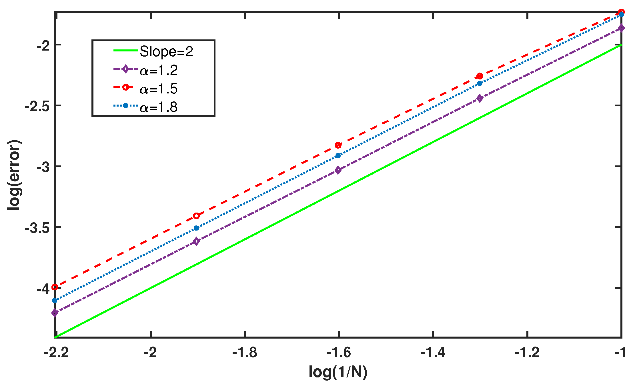
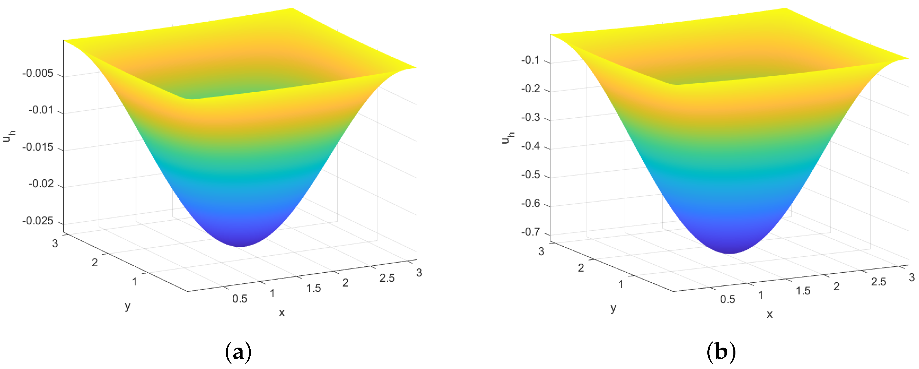
Due to the fact that the solution of this numerical example is unknown, we use the two mesh principles given in [27] to verify the theoretical result of Theorem 2. Figure 1 displays the error in time for different , where is chosen. It is shown that the rate of convergence attains the 2 order in time, as predicted by Theorem 2. Figure 2 presents the numerical solution at for . The displayed result of this figure shows that the solution of this problem behaves diffusive as , and the characteristic of the initial solution is well maintained as , which indicates that the propagation speed of waves is finite. Moreover, the attenuation of the numerical solution gradually slows down as , verifying the wave feature again.
6. Conclusions
This paper investigates the regularity result of Equation (1), which indicates that the solution behaves as a weak singularity at . In order to construct a fully discrete scheme, the nonuniform Alikhanov scheme in time is used along with the finite difference method in space. Then, the stability analysis and an -robust optimal convergent result under -norm for the proposed scheme are obtained. Finally, two numerical examples are provided to verify the theoretical result. In the future, we will extend the proposed scheme to the Equation (1) with a nonlinear term and present the unconditional optimal error estimate. In addition, we will extend the proposed scheme to fractional equations with the Caputo-Hadamard fractional derivative.
Author Contributions
Conceptualization, methodology, investigation, writing—original draft preparation, Z.A.; validation, writing—review and editing, supervision, C.H. All authors have read and agreed to the published version of the manuscript.
Funding
The research of Chaobao Huang is supported by the National Natural Science Foundation of China under grant 12101360, the Support Plan for Outstanding Youth Innovation Team in Shandong Higher Education Institutions under grant 2022KJ184, and the Natural Science Foundation of Shandong Province under grant ZR2020QA031.
Data Availability Statement
No new data were created or analyzed in this study. Data sharing is not applicable to this article.
Acknowledgments
We thank both reviewers for their careful reading of the paper, and we also would like to express our gratitude to the editor for taking time to handle the manuscript.
Conflicts of Interest
The authors declare no conflict of interest.
References
- Uchaikin, V.V. Fractional Derivatives for Physicists and Engineers; Background and theory; Nonlinear Physical Science, Higher Education Press: Beijing, China; Springer: Heidelberg, Germany, 2013; Volume I, pp. xxii+385. [Google Scholar] [CrossRef]
- Hilfer, R. (Ed.) Applications of Fractional Calculus in Physics; World Scientific Publishing Co., Inc.: River Edge, NJ, USA, 2000; pp. viii+463. [Google Scholar] [CrossRef]
- Nigmatullin, R.R. To the Theoretical Explanation of the “Universal Response”. Phys. Status Solidi (b) 1984, 123, 739–745. [Google Scholar] [CrossRef]
- Cuesta, E.; Kirane, M.; Malik, S.A. Image structure preserving denoising using generalized fractional time integrals. Signal Process. 2012, 92, 553–563. [Google Scholar] [CrossRef]
- Shallal, M.A.; Jabbar, H.N.; Ali, K.K. Analytic solution for the space-time fractional Klein-Gordon and coupled conformable Boussinesq equations. Results Phys. 2018, 8, 372–378. [Google Scholar] [CrossRef]
- Zhong, W.; Wang, L. Basic theory of initial value problems of conformable fractional differential equations. Adv. Differ. Equ. 2018, 2018, 321. [Google Scholar] [CrossRef]
- Stynes, M.; O’Riordan, E.; Gracia, J.L. Error analysis of a finite difference method on graded meshes for a time-fractional diffusion equation. SIAM J. Numer. Anal. 2017, 55, 1057–1079. [Google Scholar] [CrossRef]
- Liao, H.l.; McLean, W.; Zhang, J. A discrete Grönwall inequality with applications to numerical schemes for subdiffusion problems. SIAM J. Numer. Anal. 2019, 57, 218–237. [Google Scholar] [CrossRef]
- Kopteva, N. Error analysis of an L2-type method on graded meshes for a fractional-order parabolic problem. Math. Comp. 2021, 90, 19–40. [Google Scholar] [CrossRef]
- Hou, D.; Hasan, M.T.; Xu, C. Müntz spectral methods for the time-fractional diffusion equation. Comput. Methods Appl. Math. 2018, 18, 43–62. [Google Scholar] [CrossRef]
- Halpern, D.; Jensen, O.; Grotberg, J. A theoretical study of surfactant and liquid delivery into the lung. J. Appl. Physiol. 1998, 85, 333–352. [Google Scholar] [CrossRef]
- Myers, T.G.; Charpin, J.P. A mathematical model for atmospheric ice accretion and water flow on a cold surface. Int. J. Heat Mass Transf. 2004, 47, 5483–5500. [Google Scholar] [CrossRef]
- Gorman, D.J. Free Vibration Analysis of Beams and Shafts; John Wiley & Sons Inc.: Hoboken, NJ, USA, 1975. [Google Scholar]
- Lysaker, M.; Lundervold, A.; Tai, X.C. Noise removal using fourth-order partial differential equation with applications to medical magnetic resonance images in space and time. IEEE Trans. Image Process. 2003, 12, 1579–1590. [Google Scholar] [CrossRef] [PubMed]
- Lyu, P.; Vong, S. A symmetric fractional-order reduction method for direct nonuniform approximations of semilinear diffusion-wave equations. J. Sci. Comput. 2022, 93, 34. [Google Scholar] [CrossRef]
- An, N.; Zhao, G.; Huang, C.; Yu, X. α-robust H1-norm analysis of a finite element method for the superdiffusion equation with weak singularity solutions. Comput. Math. Appl. 2022, 118, 159–170. [Google Scholar] [CrossRef]
- Hu, X.; Zhang, L. A new implicit compact difference scheme for the fourth-order fractional diffusion-wave system. Int. J. Comput. Math. 2014, 91, 2215–2231. [Google Scholar] [CrossRef]
- Li, X.; Wong, P.J.Y. An efficient numerical treatment of fourth-order fractional diffusion-wave problems. Numer. Methods Partial. Differ. Equ. 2018, 34, 1324–1347. [Google Scholar] [CrossRef]
- Bhrawy, A.H.; Doha, E.H.; Baleanu, D.; Ezz-Eldien, S.S. A spectral tau algorithm based on Jacobi operational matrix for numerical solution of time fractional diffusion-wave equations. J. Comput. Phys. 2015, 293, 142–156. [Google Scholar] [CrossRef]
- Huang, J.; Qiao, Z.; Zhang, J.; Arshad, S.; Tang, Y. Two linearized schemes for time fractional nonlinear wave equations with fourth-order derivative. J. Appl. Math. Comput. 2021, 66, 561–579. [Google Scholar] [CrossRef]
- Ran, M.; Lei, X. A fast difference scheme for the variable coefficient time-fractional diffusion wave equations. Appl. Numer. Math. 2021, 167, 31–44. [Google Scholar] [CrossRef]
- An, Y.; Liu, R. Existence of nontrivial solutions of an asymptotically linear fourth-order elliptic equation. Nonlinear Anal. 2008, 68, 3325–3331. [Google Scholar] [CrossRef]
- Shen, J.; Stynes, M.; Sun, Z.Z. Two Finite Difference Schemes for Multi-Dimensional Fractional Wave Equations with Weakly Singular Solutions. Comput. Methods Appl. Math. 2021, 21, 913–928. [Google Scholar] [CrossRef]
- Huang, C.; Chen, H.; An, N. β-robust superconvergent analysis of a finite element method for the distributed order time-fractional diffusion equation. J. Sci. Comput. 2022, 90, 44. [Google Scholar] [CrossRef]
- Alikhanov, A.A. A new difference scheme for the time fractional diffusion equation. J. Comput. Phys. 2015, 280, 424–438. [Google Scholar] [CrossRef]
- Chen, H.; Stynes, M. Blow-up of error estimates in time-fractional initial-boundary value problems. IMA J. Numer. Anal. 2020, 41, 974–997. [Google Scholar] [CrossRef]
- Farrell, P.A.; Hegarty, A.F.; Miller, J.J.H.; O’Riordan, E.; Shishkin, G.I. Robust Computational Techniques for Boundary Layers; Applied Mathematics (Boca Raton); Chapman & Hall/CRC: Boca Raton, FL, USA, 2000; Volume 16, pp. xvi+254. [Google Scholar]
Figure 1.
The plot of error for .

Figure 2.
The numerical solution for Example 2 at . (a) ; (b) .


Table 1.
Convergent results of in temporal direction with .
| N = 20 | N = 40 | N = 80 | N = 160 | N = 320 | |
|---|---|---|---|---|---|
| 3.4823 | 9.1635 | 2.3618 | 5.9906 | 1.5053 | |
| 1.9261 | 1.9959 | 1.9791 | 1.9925 | ||
| 3.2409 | 8.3604 | 2.1279 | 5.3611 | 1.3425 | |
| 1.9547 | 1.9740 | 1.9888 | 1.9976 | ||
| 3.1744 | 8.1407 | 2.0645 | 5.1916 | 1.2969 | |
| 1.9632 | 1.9793 | 1.9915 | 2.0010 |
Table 2.
Convergent results of in spatial direction.
| 9.9170 | 2.4773 | 6.1757 | 1.5528 | |
| 2.0014 | 2.0040 | 1.9917 | ||
| 9.9080 | 2.4771 | 6.1970 | 1.5699 | |
| 1.9999 | 1.9990 | 1.9836 | ||
| 1.0077 | 2.5205 | 6.3258 | 1.6172 | |
| 1.9993 | 1.9943 | 1.9677 |
Disclaimer/Publisher’s Note: The statements, opinions and data contained in all publications are solely those of the individual author(s) and contributor(s) and not of MDPI and/or the editor(s). MDPI and/or the editor(s) disclaim responsibility for any injury to people or property resulting from any ideas, methods, instructions or products referred to in the content. |
© 2024 by the authors. Licensee MDPI, Basel, Switzerland. This article is an open access article distributed under the terms and conditions of the Creative Commons Attribution (CC BY) license (https://creativecommons.org/licenses/by/4.0/).
Share and Cite
MDPI and ACS Style
An, Z.; Huang, C. Error Analysis of the Nonuniform Alikhanov Scheme for the Fourth-Order Fractional Diffusion-Wave Equation. Fractal Fract. 2024, 8, 106. https://doi.org/10.3390/fractalfract8020106
AMA Style
An Z, Huang C. Error Analysis of the Nonuniform Alikhanov Scheme for the Fourth-Order Fractional Diffusion-Wave Equation. Fractal and Fractional. 2024; 8(2):106. https://doi.org/10.3390/fractalfract8020106
Chicago/Turabian StyleAn, Zihao, and Chaobao Huang. 2024. "Error Analysis of the Nonuniform Alikhanov Scheme for the Fourth-Order Fractional Diffusion-Wave Equation" Fractal and Fractional 8, no. 2: 106. https://doi.org/10.3390/fractalfract8020106