

Space–Time Variations in the Long-Range Dependence of Sea Surface Chlorophyll in the East China Sea and the South China Sea


1
Ocean College, Zhejiang University, Zhoushan 316021, China
2
Joint Center for Blue Carbon Research, Ocean Academy, Zhejiang University, Zhoushan 316021, China
3
Ocean Research Center of Zhoushan, Zhejiang University, Zhoushan 316021, China
4
East China Normal University, Shanghai 200062, China
*
Author to whom correspondence should be addressed.
Fractal Fract. 2024, 8(2), 102; https://doi.org/10.3390/fractalfract8020102
Submission received: 28 December 2023
/
Revised: 1 February 2024
/
Accepted: 6 February 2024
/
Published: 7 February 2024
(This article belongs to the Special Issue Fractional Processes and Systems in Computer Science and Engineering)
Abstract
:Gaining insights into the space–time variations in the long-range dependence of sea surface chlorophyll is crucial for the early detection of environmental issues in oceans. To this end, 12 locations were selected along the Yangtze River and Pearl River estuaries, varying in distances from the Chinese coastline. Daily satellite-observed sea surface chlorophyll concentration data at these 12 locations were collected from the Copernicus Marine Service website, spanning from December 1997 to November 2023. The main objective of the current study is to introduce a multi-fractional generalized Cauchy model for calculating the values of Hurst exponents and quantitatively assessing the long-range dependence strength of sea surface chlorophyll at different spatial locations and time instants during the study period. Furthermore, ANOVA was utilized to detect the differences of calculated Hurst exponent values among the locations during various months and seasons. From a spatial perspective, the findings reveal a significantly stronger long-range dependence of sea surface chlorophyll in offshore regions compared to nearshore areas, with Hurst exponent values > 0.5 versus <0.5. It is noteworthy that the values of Hurst exponents at each location exhibit significant differences during various seasons, from a temporal perspective. Specifically, the long-range dependence of sea surface chlorophyll in summer in the nearshore region is weaker than in other seasons, whereas that in the offshore region is stronger than in other seasons. The study concludes that long-range dependence is inversely related to the distance from the coastline, and anthropogenic activity plays a dominant role in shaping the long-range dependence of sea surface chlorophyll in the coastal regions of China.
1. Introduction
Chlorophyll plays a pivotal role as a pigment in the photosynthetic processes of phytoplankton and algae, providing crucial insights into the growth conditions of marine vegetation [1]. Monitoring the concentration of chlorophyll on the sea’s surface serves is a valuable tool for assessing water quality [2], particularly in relation to nutrient levels. Anomalous chlorophyll concentrations can cause ecosystem changes, such as eutrophication and occurrences of cyanobacterial blooms, often attributed to human activities, agricultural runoff, and urban pollution. Notably, the urbanization of coastlines results in elevated nutrient inputs into coastal seas, contributing to a higher frequency of red tide events [3]. The city lockdown policy during the COVID-19 pandemic contributed to the increment in sea surface chlorophyll in Bohai Sea (China) [4]. The research unveiled the significant impacts of human activities on sea surface chlorophyll concentrations in China’s Yangtze and Pearl River estuaries [5,6]. The vigilant monitoring of sea surface chlorophyll concentration variations contributes to the early detection of environmental issues, enabling the implementation of timely and appropriate protective measures.
The growth of phytoplankton and algae is a continuous process, inevitably leading to a consistent variation in chlorophyll concentration over time. This phenomenon is specifically observed through the autocorrelation properties of the chlorophyll concentration time series. For instance, significant positive autocorrelations persist from one month to the next across almost all ocean regions [7]. In the Gulf of California, the satellite-observed sea surface chlorophyll exhibits a robust autocorrelation feature throughout various temporal spans during warm and cold seasons [8]. Moreover, diverse variability features in autocorrelation are evident in different seas of China [9]. Specifically, long-range dependence with a strong autocorrelation result was detected in the South China Sea [10]. Scholars have employed long short-term memory neural networks (LSTMs) with temporal correlation properties to precisely predict chlorophyll concentrations, indirectly highlighting the autocorrelation characteristics of chlorophyll concentrations [1]. Moreover, by integrating the capabilities of LSTM, a spatial–temporal attention network was developed to forecast chlorophyll levels in the Xiamen Sea (China), surpassing the performance of the independent LSTM model [11]. Similarly, the Ca-STANet framework, incorporating spatial attention feature extraction, temporal attention feature extraction modules, along with spatio-temporal input preprocessing and spatio-temporal fusion prediction modules, was introduced to accurately predict chlorophyll levels in the Bohai Sea (China) [12].
He [13] modeled the autocorrelation function of sea surface chlorophyll concentrations using a generalized Cauchy model. Utilizing the Hurst exponent, the author quantified the autocorrelation characteristics of sea surface chlorophyll concentrations and found that sea surface chlorophyll exhibited long-range dependence. Furthermore, the long-term analysis of global sea surface chlorophyll concentrations indicated weaker long-range dependence in nearshore areas and stronger long-range dependence in offshore regions [14,15]. By combining the historical trends of sea surface chlorophyll concentrations and leveraging their long-range dependence characteristics, accurate trend forecasting becomes possible [16]. Obtaining insights into the temporal variability in the long-range dependence features of sea surface chlorophyll concentrations can enhance the accuracy of the forecasting process.
Mono-fractals can fail in providing a comprehensive description of natural patterns, particularly when attempting to capture the nuanced temporal variations governed by natural laws. In such cases, multi-fractals offer a promising methodology. The spatial distribution multi-fractal characteristics of sea surface chlorophyll were detected in several studies and revealed that turbulent mixing could be the dominant factor of phytoplankton distribution [17,18,19]. However, a noticeable gap persists in the research focusing on quantifying the multi-fractal features of sea surface chlorophyll from a temporal perspective. Peltier and Véhel [20] formulated a model for multi-fractional Brownian motion. Introducing the concept of moving time windows, they innovatively proposed a method for calculating local Hurst exponents. Expanding on this foundation, the researchers [21,22,23] extended the algorithm to encompass multi-fractional Gaussian noise models and multi-fractional generalized Cauchy models. Their studies demonstrated that network traffic and sea surface height fluctuations exhibited the long-range dependence properties of multi-fractal models, as evidenced by the fluctuations in the Hurst exponent over time. Moreover, Hu et al. [24] utilized a multi-fractional Gaussian noise model to analyze the sound time series of giant pandas, revealing that this sequence also displayed long-range dependence properties of multi-fractal models. However, limited attention has been directed towards investigating the instantaneous fractal or multi-fractional characteristics of sea surface chlorophyll concentrations.
In view of the above mentioned considerations, the main objectives of the current study are twofold: (1) using a multi-fractional generalized Cauchy model to explore the multi-fractional characteristics of sea surface chlorophyll, i.e., the long-range dependence characteristic; and (2) detecting the temporal variability of the long-range dependence and exploring the impact of anthropogenic activity on the properties.
2. Materials and Methods
2.1. Data Collection
Long-term daily sea surface chlorophyll concentration data were downloaded from the Copernicus website (https://data.marine.copernicus.eu/product/OCEANCOLOUR_GLO_BGC_L4_MY_009_104/description, accessed on 10 December 2023). It merges the data from multi-sourced satellite sensors, including SeaWiFS (Sea-Viewing Wide Field of View Sensor), MODIS (Moderate Resolution Imaging Spectroradiometer)-Aqua & Terra, MERIS (Medium-Resolution Imaging Spectrometer), and VIIRS (Visible and Infrared Imager/Radiometer Suite)-SNPP & JPSS1, OLCI (Ocean and Land Color Instrument)-S3A & S3B. To ensure completeness, a space–time interpolation method was applied to generate gap-free Copernicus products with a spatial resolution of 4 km and a temporal resolution of one day. The in situ sea surface chlorophyll observations from Argo buoys were also downloaded from https://dataselection.euro-argo.eu/ (accessed on 10 December 2023) and collected for validation, and the results showed that the mean absolute error of the Copernicus products was 0.1264 mg/m3.
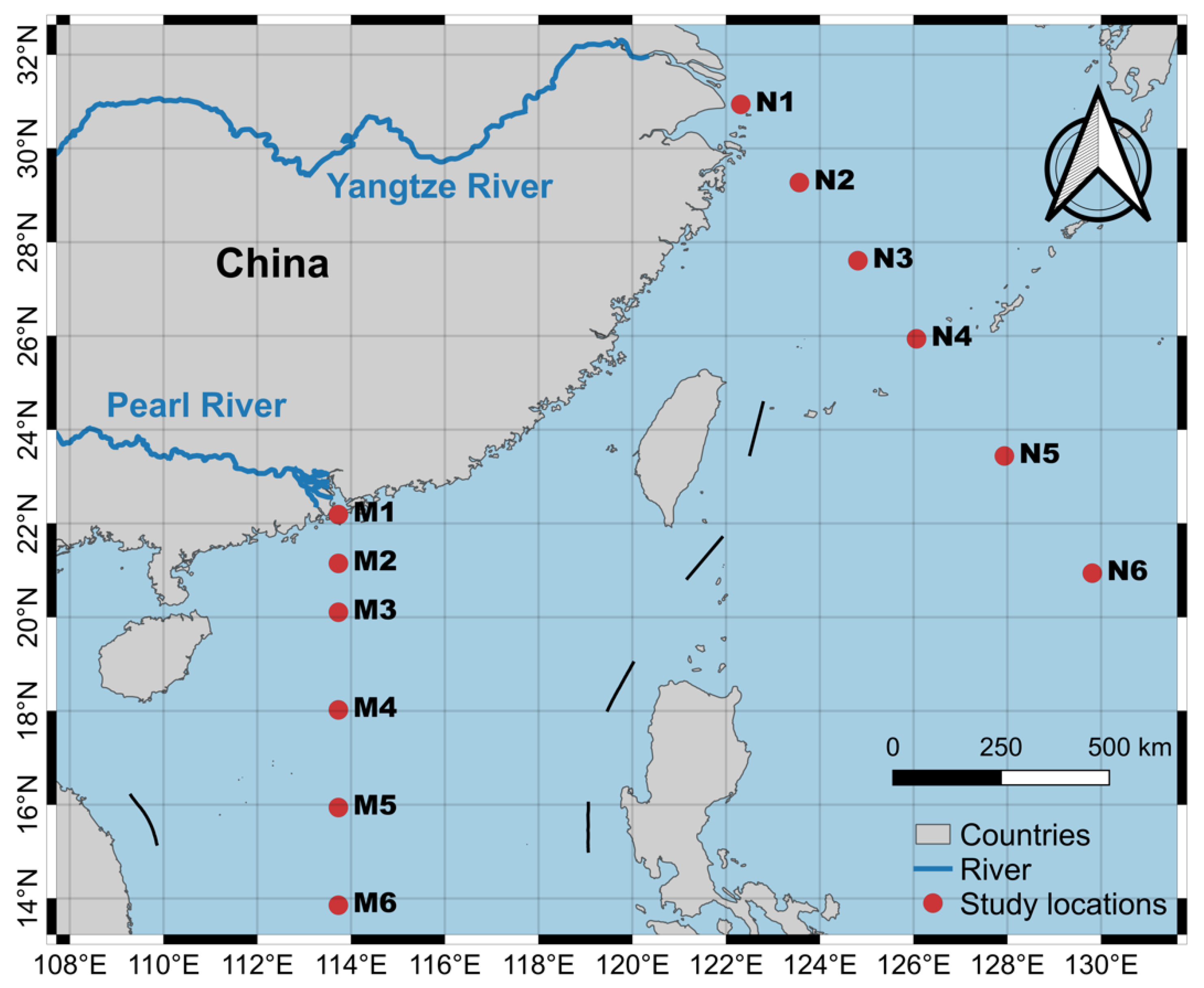
In the present study, twelve points were selected at varying distances from the coastline in the coastal regions of China, as shown in Figure 1. Among them, M1, M2, …, M6 were located on the outer region of the Pearl River estuary, while N1, N2, …, N6 were located on the outer region of the Yangtze River estuary. The Yangtze River, holding the distinction of being the largest river in Eurasia, boasts an impressive length of 6300 km, an expansive catchment area spanning 1.8 million square kilometers, and a human population exceeding 400 million within its extensive catchment region [25]. Meanwhile, the Pearl River, renowned for its significance in southern China, stands as the third-longest river in the country, with an approximate length of 2400 km. The time series of the sea surface chlorophyll concentration was extracted for the multi-fractal analysis during the period from 1 December 1997 to 30 November 2023, encompassing a total of 26 years (9496 days).
2.2. Methodology
2.2.1. The Cauchy Distribution
The Cauchy distribution is a case of the heavy-tailed probability density function, which can be written as Equation (1):
where and are the location and scale parameter, respectively. Without losing generality, Equation (1) can be simplified by setting the following values: and . Thus, it becomes:
The mean, , and variance, , values of the Cauchy distribution have the characteristics displayed in Equations (3) and (4):
In this case, the mean or variance of the Cauchy distribution may not exist, which is a typical feature of a heavy-tailed distribution in terms of Taqqu’s law [26,27]. Therefore, the Hurst exponent and fractal dimension were utilized instead of the mean and variance for describing the features of the considered fractal time series. Furthermore, the heavy-tailed distribution of a time series, , leads to the long-range dependence characteristics of [22,28,29].
2.2.2. Multi-Fractional Generalized Cauchy Model
The generalized Cauchy model can simultaneously capture the independent variations in the Hurst exponent and fractal dimension parameters by modeling the autocorrelation function of a time series [22]. Specifically, the normalized autocorrelation function of a time series, , can be written as Equation (5), if it satisfies the generalized Cauchy process [22,30]:
where and denote the Hurst exponent and fractal dimension, respectively, representing the long-range dependence and self-similarity of the time series, . The ranges of the two parameters are and . When , it represents long-range dependence, whereas when , it represents a short-range dependence. Then, the normalized autocorrelation function of the multi-fractional generalized Cauchy model can be written as Equation (6), according to the literature [22]:
where and ; similar definitions of long-range dependence and short-range dependence were applied to . In this case, and . When , the autocorrelation function becomes:
Specifically, for , is well approximated by . Given this approximation, the autocorrelation function of the multi-fractional generalized Cauchy model is equivalent to that of the modified multi-fractional Gaussian noise for large [23]. Hence, can be obtained by using the computation process presented in the literature [20], shown in Equations (8) and (9):
where is the number of data; is the length of the neighborhood data used for estimating the Hurst exponent; and m is the largest integer smaller than . In the current study, is set to 14 days, and the series values of sea surface chlorophyll concentrations at the 12 studied locations were calculated. The sea surface chlorophyll concentration can change significantly during the short bloom period, and the corresponding calculated values can be close to 0. On the other hand, when the sea surface chlorophyll concentration remains stable, the calculated values are close to 1. Previous studies have shown that the self-similarity of sea surface chlorophyll is rather weak [13,14,15]. Therefore, the current study only focused on the long-range dependence variations in sea surface chlorophyll.
The power spectrum density (PSD) of the multi-fractional generalized Cauchy model can be written as Equation (10) [22]:
where F is the operator of the Fourier transformation, and for the multi-fractional generalized Cauchy model with a long-range dependence, Equation (10) can be further expressed as Equation (11):
2.2.3. Statistical Analysis
The analysis of variance (ANOVA) was implemented to distinguish the differences among various series at corresponding locations, as well as the monthly and seasonal variations in . Specifically, the least-significant difference (LSD) test was employed for comparing the averaged values among various groups of data. It was developed by Fisher in 1935 for pairwise comparisons by computing the smallest significant difference (i.e., LSD) between two means and identifying the populations whose means were statistically different [31]. More detailed information on the LSD can be found in the literature [31,32].
3. Results
3.1. Descriptive Statistics of Sea Surface Chlorophyll Concentration Series
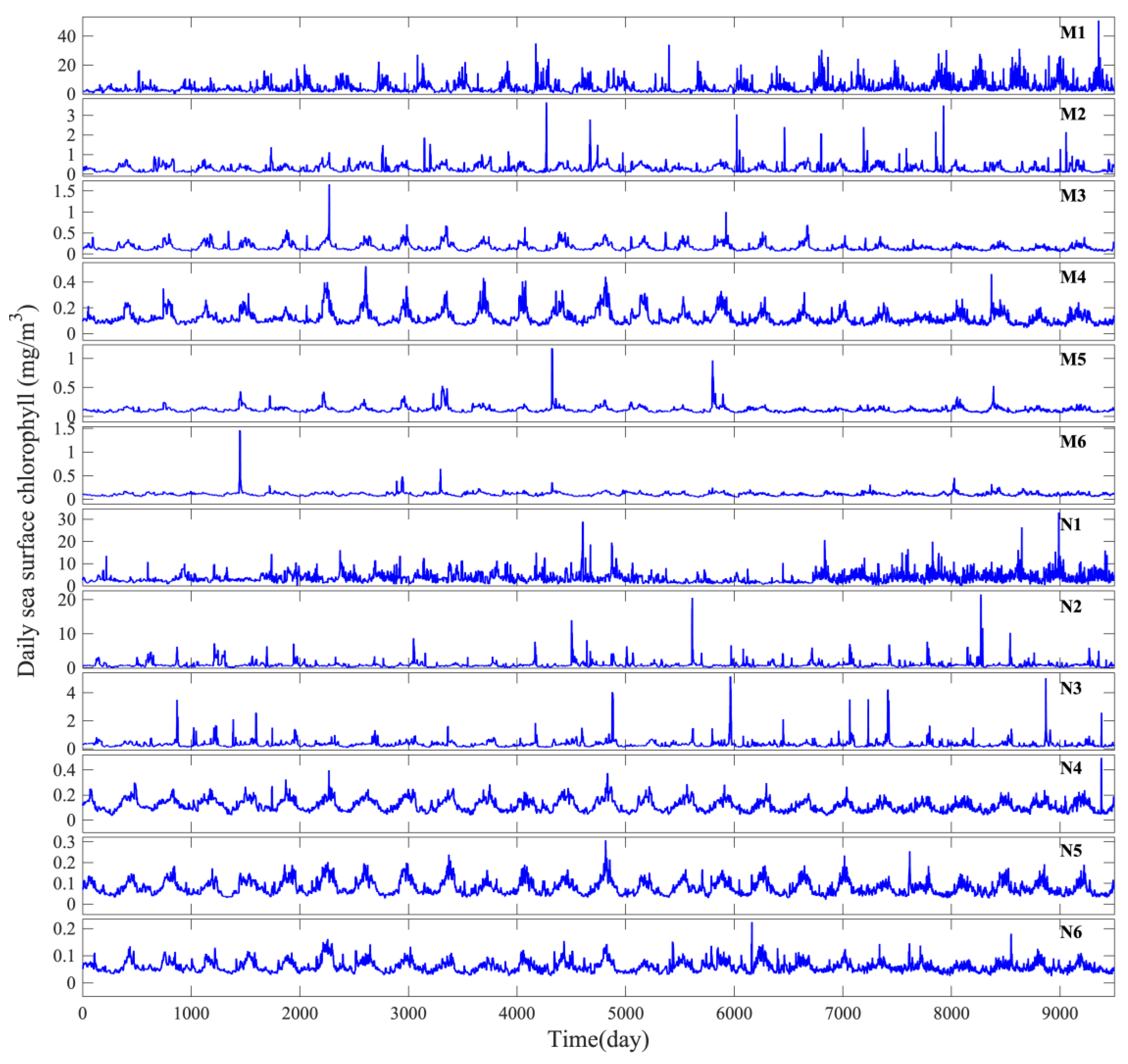
The daily sea surface chlorophyll concentrations at the 12 studied locations are plotted in Figure 2, and the descriptive statistical results are presented in Table 1. The statistical results indicate that the sea surface chlorophyll concentrations present the highest ranges at the M1 and N1 locations, i.e., 0.1356–50.8658 mg/m3 and 0.0932–33.0401 mg/m3, respectively, among the two groups of data, which are the closest locations to the Pearl River estuary and Yangtze River estuary. The range of the sea surface chlorophyll concentration decreases with distance concerning to the two estuaries. Moreover, the mean values and standard deviation values had the similar decreasing trends from the estuaries to offshore locations. According to the LSD-t results, there are significant differences in the mean sea surface chlorophyll concentration values among M1, M2, M3, and M6 at a 0.05 significance level. Conversely, the mean values of M3, M4, and M5 (or M4, M5, and M6) do not exhibit significant differences at the 0.05 significance level. On another note, the mean sea surface chlorophyll concentration values at N1, N2, N3, N4, and N5 (or N6) display significant variations, while the mean values at N5 and N6 do not differ significantly from each other at the 0.05 significance level.
3.2. Variability of the Long-Range Dependence of Sea Surface Chlorophyll Series
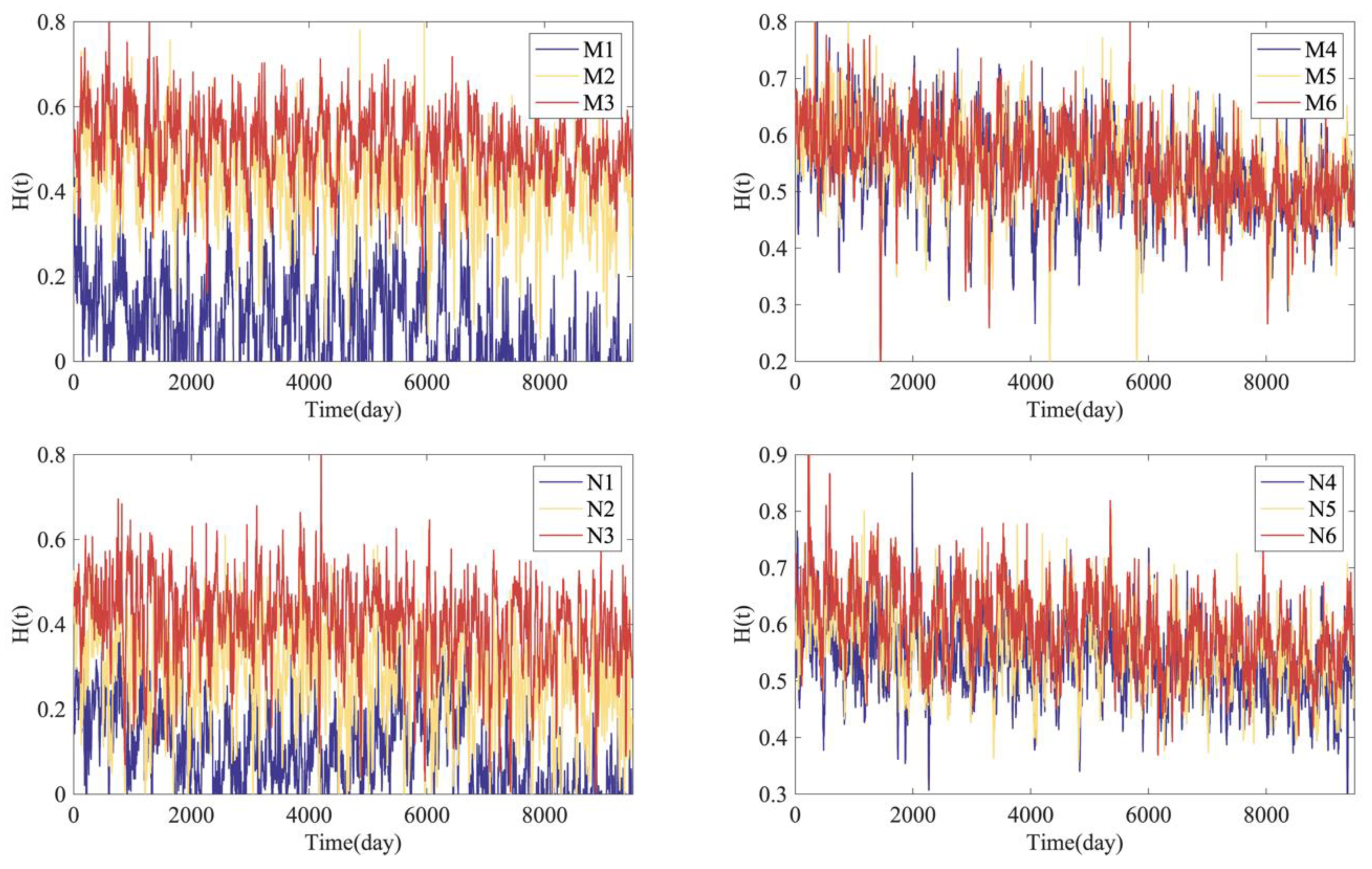
The variations in the Hurst exponents for sea surface chlorophyll series across the 12 examined locations are depicted in Figure 3, with the corresponding statistical findings presented in Table 1. Notably, the curve values for Hurst exponents at M1, M2, and M3 (or N1, N2, and N3) appear to be distinct from one another, whereas the values for Hurst exponents at M4, M5, and M6 (or N4, N5, or N6) overlap. The mean Hurst exponent values exhibit an increasing trend from M1 to M6 (from 0.0522 to 0.5431) and from N1 to N6 (from 0.0829 to 0.5909), respectively, indicating that the Hurst exponent values increase with the distance from the coastline. Specifically, the mean Hurst exponent values are lower than 0.5 at the M1, M2, N1, N2, and N3 locations, indicating a short-range dependence. Conversely, the mean Hurst exponent values are greater than 0.5 at the M3, M4, M5, M6, N4, N5, and N6 locations, suggesting a long-range dependence. According to the LSD test results, the mean Hurst exponent values for M1–M6 and N1–N6 are all significantly different from each other at a 0.05 significance level.
3.3. Monthly and Seasonal Variations in Hurst Exponents for Sea Surface Chlorophyll
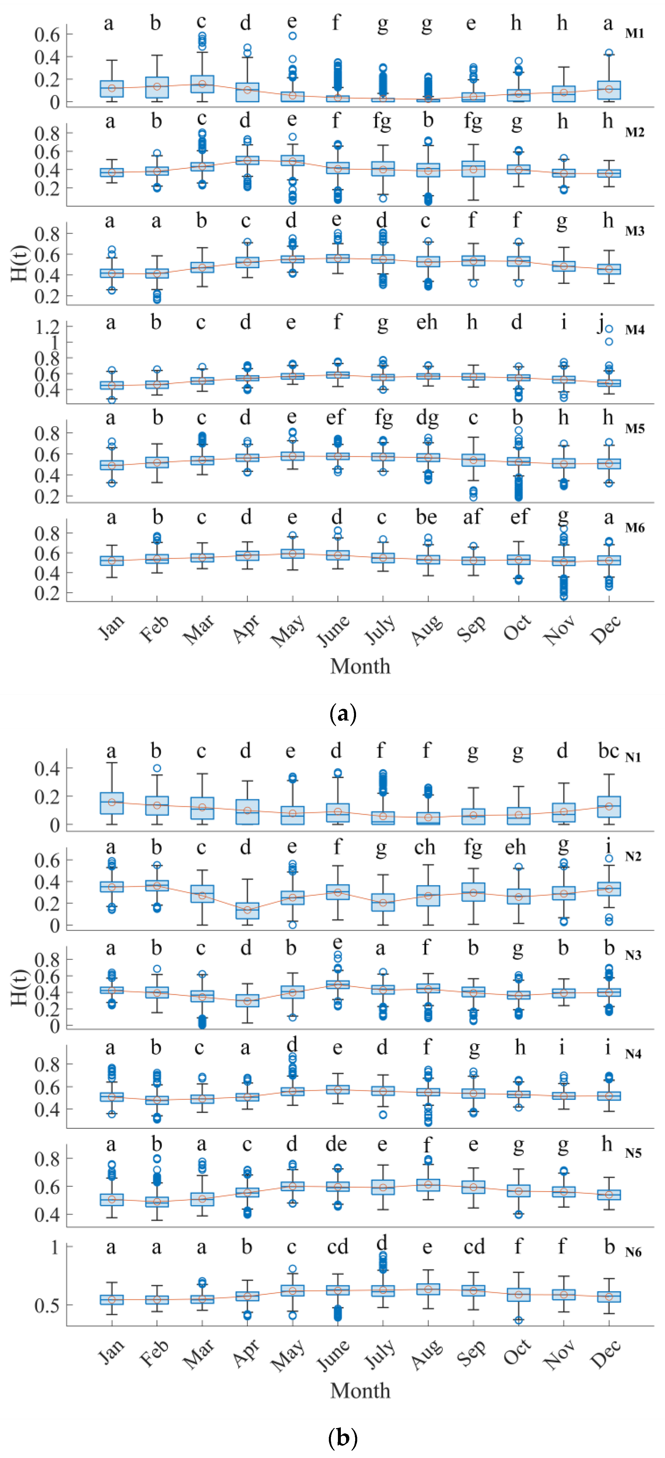
Figure 4 illustrates the monthly fluctuations in the Hurst exponents for sea surface chlorophyll across the 12 studied locations. Upon comparing trends among different locations, distinct patterns emerge. For instance, at the M1 location, the Hurst exponent values exhibit an increasing–decreasing–increasing trend from January to December. At the M2 and M3 locations, the trend is characterized by an increasing–decreasing–stable–decreasing pattern. Conversely, at the M4, M5, and M6 locations, the Hurst exponent values follow a simple increasing–decreasing trajectory. Likewise, the Hurst exponent values for the N1 location demonstrate a consistent decreasing–increasing pattern from January to December. Notably, the N2 and N3 locations reveal a more intricate trend, characterized by a decreasing–increasing–decreasing–increasing sequence of Hurst exponent values. Contrastingly, the N4 and N5 locations exhibit a straightforward decreasing–increasing–decreasing trend. The Hurst exponent values at the N6 location portray a stable–increasing–decreasing trend.
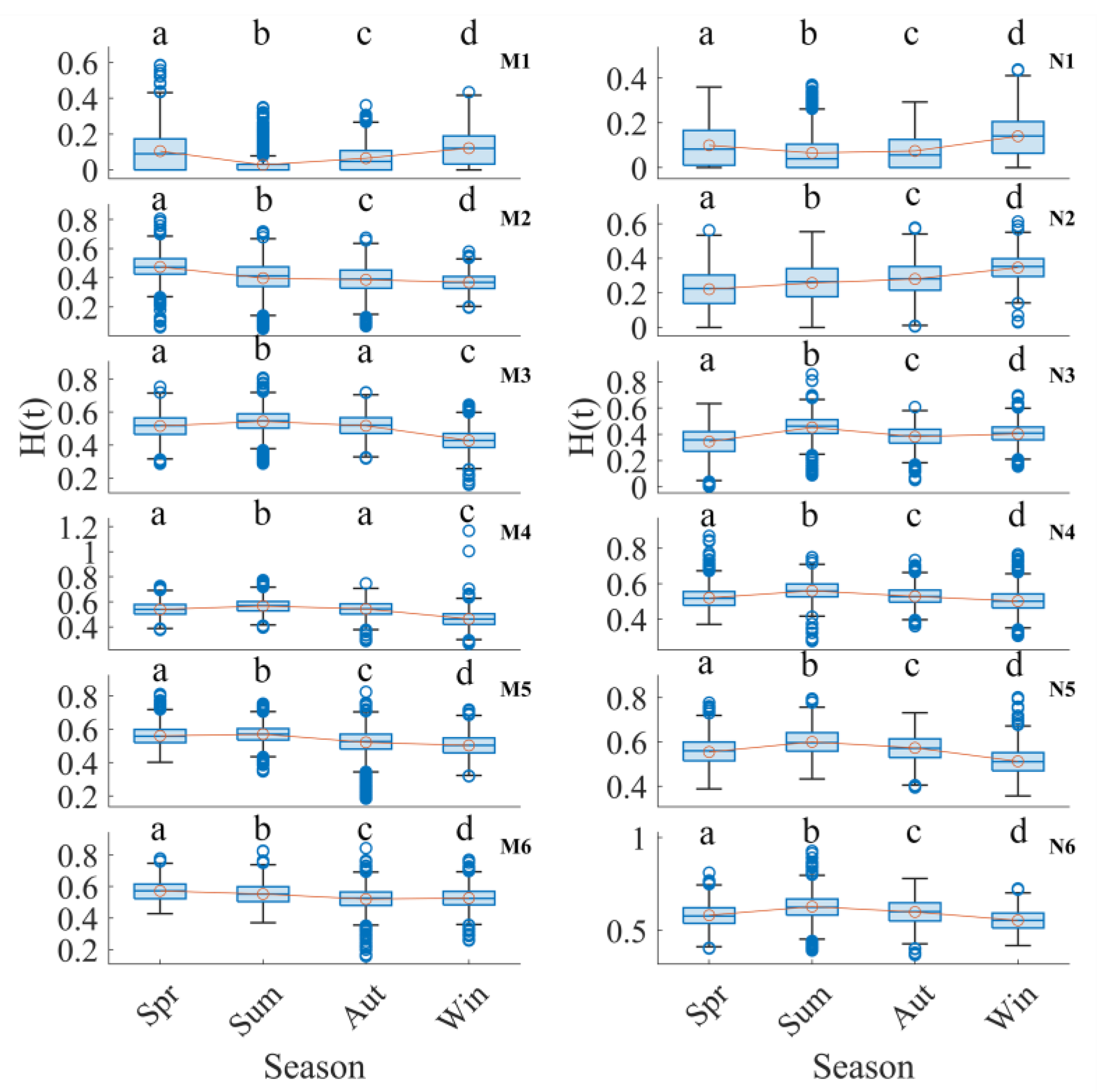
Furthermore, the seasonal variations in the Hurst exponent values across different locations are compared and depicted in Figure 5. Utilizing the LSD test, the Hurst exponent values at the M1, M2, M5, M6, N1, N2, …, N6 locations exhibited statistically significant seasonal differences at the 0.05 significance level. Conversely, for the M3 and M4 locations, the Hurst exponent values demonstrated similarities during the spring and autumn seasons at the 0.05 significance level. To elaborate, a discernible decreasing–increasing trend in the Hurst exponent values was identified at the M1 location from spring to winter seasons, while a simple decreasing trend was observed at the M2 location. Meanwhile, the Hurst exponent values at the M3, M4, and M5 locations manifested a similar increasing–decreasing pattern. Additionally, a decreasing–stable trend characterized the Hurst exponent values at the M6 location. Concerning the N locations, N1 exhibited a discernible decreasing–increasing trend, while N2 displayed a consistent increasing trend from spring to winter. In contrast, the remaining four locations demonstrated a trend characterized by an initial increase followed by a subsequent decrease in the Hurst exponent values.
4. Discussion
The present study employed multi-fractional generalized Cauchy model to characterize the temporal variations in Hurst exponents at 12 locations in the coastal regions of China during a 26-year period, which served as indicators of the long-range dependence of sea surface chlorophyll concentrations. The overall trend and the seasonal and monthly variabilities at the various locations in Chinese coastal regions were observed and detected.
4.1. The Impact of Anthropogenic Activity on the Long-Range Dependence of Sea Surface Chlorophyll Concentration
The nutrient levels in the waters of the Yangtze River estuary region have shifted from being climate-driven to being anthropogenic activity-driven since the 1950s [33]. As a major agricultural nation, fertilizers were extensively used to promote the growth and increase the yield of crops in China [34]. Studies indicate that this agricultural non-point source pollution will enter the Yangtze River through surface runoff and eventually reach the East China Sea, leading to an elevation in nutrient concentrations. Except for the fertilizer usage, sewage discharge, detergent application, livestock breeding, etc., will also contribute to the nutrient load from the Yangtze River entering the East China Sea [35]. Specifically, 36% of the total nitrogen and 63% of the total phosphorus inputs in the East China Sea originate from agricultural non-point source pollution [25]. A total of 4.62 Gg of TN and 0.27 Gg of TP entered the East China Sea per day from the Yangtze River, on average [36]. This resulted in a significant proliferation of algae in the East China Sea. In 2022 alone, there were 29 occurrences of red tide outbreaks in the East China Sea [37]. Similarly, the research has found that the eutrophication intensity in the Pearl River Estuary has been gradually increasing since the 1970s, influenced by anthropogenic activity [38]. The impacts of anthropogenic activities on the nutrient levels in the Yangtze River estuary and Pearl River estuary diminish with an increasing distance from the coastline, resulting in a gradient decreasing distribution pattern of nutrients from the coastline [39,40,41,42]. Elevated nutrient concentrations contribute to a heightened variability in sea surface chlorophyll levels, leading to increased occurrences of algae and phytoplankton blooms. Consequently, the long-range dependence weakens and the Hurst exponents register lower values. In turn, the low nutrient levels at the offshore regions lead to strong long-range dependence and high Hurst exponent values (Figure 3 and Table 1).
4.2. Seasonal Variation in the Long-Range Dependence of Sea Surface Chlorophyll Concentration
During summer, nutrients exhibit heightened activity in the Yangtze River estuary, resulting in smaller Hurst exponents and a diminished strength of long-range dependence compared to other seasons [43]. On the other hand, the southwesterly summer monsoon induces strong upwelling in the coastal regions of China [44], facilitating the transport of nutrients from the ocean floor to the sea surface. This phenomenon promotes the flourishing growth of algae and phytoplankton, and increases the variability in sea surface chlorophyll levels with low-value Hurst exponents. This could be the reason why Hurst exponents exhibit high levels in the coastal regions of China, i.e., M1 and N1 locations (Figure 5). On the other hand, the temperature in summer favors the continuous growth in the offshore regions, such as the M3, M4, M5, N3, N4, N5, and N6 locations; however, without sufficient nutrients, the growth rate is weak and leads to a strong long-range dependence characterized by high-value Hurst exponents.
4.3. Limitations and Future Work
Certain limitations of the current study should be acknowledged: (1) in the absence of long-term in situ-measured sea surface chlorophyll data, remote sensing data with some uncertainties were utilized, especially for the nearshore regions [15,45]. Therefore, the characterized space–time variations in the long-range dependence also presented uncertainties. (2) Qualitative analyses and inferences were conducted to explain the impact of anthropogenic activity on the space–time long-range dependence of sea surface chlorophyll, and future work should focus on quantitative analyses by collecting nutrient data.
5. Conclusions
The space–time variations in the long-range dependence values of sea surface chlorophyll levels were investigated using the multi-fractional generalized Cauchy model in 12 locations in the coastal regions of China over a 26-year period. The results indicate that proximity to the estuaries of the Yangtze River and Pearl River correlate with weaker long-range dependence values of sea surface chlorophyll levels. In contrast, the offshore regions exhibit consistently strong long-range dependence values throughout the study period. Additionally, seasonal variations revealed opposing long-range dependence patterns between nearshore and offshore areas during summer. In essence, anthropogenic activities were identified as the dominant factor influencing the long-range dependence of sea surface chlorophyll. Future work should focus on quantifying the impacts of anthropogenic activities on the long-range dependence of sea surface chlorophyll. The present workflow can also be applied to other types of fractional derivatives.
Author Contributions
Conceptualization, J.H. and M.L.; methodology, J.H. and M.L.; software, J.H.; validation, J.H.; formal analysis, J.H.; investigation, J.H.; resources, J.H.; data curation, J.H.; writing—original draft preparation, J.H.; writing—review and editing, J.H. and M.L.; visualization, J.H.; supervision, J.H. and M.L.; project administration, J.H.; funding acquisition, J.H. All authors have read and agreed to the published version of the manuscript.
Funding
This work is supported by the National Natural Science Foundation of China (Grant Nos. 42301374 and 42171398), National Key R&D Program of China (Grant No. 2023YFE0113103), and Zhejiang Provincial Natural Science Foundation of China (Grant No. LDT23D06024D06).
Data Availability Statement
The data resources are provided in the main text.
Conflicts of Interest
The authors declare no conflicts of interest.
References
- Na, L.; Shaoyang, C.; Zhenyan, C.; Xing, W.; Yun, X.; Li, X.; Yanwei, G.; Tingting, W.; Xuefeng, Z.; Siqi, L. Long-Term Prediction of Sea Surface Chlorophyll-a Concentration Based on the Combination of Spatio-Temporal Features. Water Res. 2022, 211, 118040. [Google Scholar] [CrossRef]
- Katlane, R.; El Kilani, B.; Dhaoui, O.; Kateb, F.; Chehata, N. Monitoring of Sea Surface Temperature, Chlorophyll, and Turbidity in Tunisian Waters from 2005 to 2020 Using MODIS Imagery and the Google Earth Engine. Reg. Stud. Mar. Sci. 2023, 66, 103143. [Google Scholar] [CrossRef]
- Nichol, J.E.; Bilal, M.; Nazeer, M.; Wong, M.S. Urban Pollution. In Urban Informatics; Shi, W., Goodchild, M.F., Batty, M., Kwan, M.-P., Zhang, A., Eds.; The Urban Book Series; Springer: Singapore, 2021; pp. 243–258. ISBN 9789811589836. [Google Scholar]
- Xiao, X.; Huang, S.; He, J. The Impact of COVID-19 Lockdown on the Variation of Sea Surface Chlorophyll-a in Bohai Sea, China. Reg. Stud. Mar. Sci. 2023, 66, 103163. [Google Scholar] [CrossRef]
- Chen, C.; Jiang, H.; Zhang, Y. Anthropogenic Impact on Spring Bloom Dynamics in the Yangtze River Estuary Based on SeaWiFS Mission (1998–2010) and MODIS (2003–2010) Observations. Int. J. Remote Sens. 2013, 34, 5296–5316. [Google Scholar] [CrossRef]
- Niu, L.; Luo, X.; Hu, S.; Liu, F.; Cai, H.; Ren, L.; Ou, S.; Zeng, D.; Yang, Q. Impact of Anthropogenic Forcing on the Environmental Controls of Phytoplankton Dynamics between 1974 and 2017 in the Pearl River Estuary, China. Ecol. Indic. 2020, 116, 106484. [Google Scholar] [CrossRef]
- Feng, J.; Durant, J.M.; Stige, L.C.; Hessen, D.O.; Hjermann, D.Ø.; Zhu, L.; Llope, M.; Stenseth, N.C. Contrasting Correlation Patterns between Environmental Factors and Chlorophyll Levels in the Global Ocean. Glob. Biogeochem. Cycles 2015, 29, 2095–2107. [Google Scholar] [CrossRef]
- Hakspiel-Segura, C.; Martínez-López, A.; Antonio Delgado-Contreras, J.; Robinson, C.J.; Gómez-Gutiérrez, J. Temporal Variability of Satellite Chlorophyll-a as an Ecological Resilience Indicator in the Central Region of the Gulf of California. Prog. Oceanogr. 2022, 205, 102825. [Google Scholar] [CrossRef]
- Zhang, K.; Zhao, X.; Xue, J.; Mo, D.; Zhang, D.; Xiao, Z.; Yang, W.; Wu, Y.; Chen, Y. The Temporal and Spatial Variation of Chlorophyll a Concentration in the China Seas and Its Impact on Marine Fisheries. Front. Mar. Sci. 2023, 10, 1212992. [Google Scholar] [CrossRef]
- Zhan, H.; Shi, P.; Mao, Q.; Zhang, T. Long-Range Correlations in Remotely Sensed Chlorophyll in the South China Sea. Chin. Sci. Bull. 2006, 51, 45–49. [Google Scholar] [CrossRef]
- He, X.; Shi, S.; Geng, X.; Xu, L.; Zhang, X. Spatial-Temporal Attention Network for Multistep-Ahead Forecasting of Chlorophyll. Appl. Intell. 2021, 51, 4381–4393. [Google Scholar] [CrossRef]
- Ye, M.; Li, B.; Nie, J.; Qian, Y.; Yang, L.-L. Ca-STANet: Spatiotemporal Attention Network for Chlorophyll-a Prediction With Gap-Filled Remote Sensing Data. IEEE Trans. Geosci. Remote Sens. 2023, 61, 4203314. [Google Scholar] [CrossRef]
- He, J. Application of Generalized Cauchy Process on Modeling the Long-Range Dependence and Self-Similarity of Sea Surface Chlorophyll Using 23 Years of Remote Sensing Data. Front. Phys. 2021, 9, 551. [Google Scholar] [CrossRef]
- He, J.; Gao, Z.; Jiang, Y.; Li, M. Spatially Heterogeneity of Long-Range Dependence and Self-Similarity of Global Sea Surface Chlorophyll Concentration with Their Environmental Factors Analysis. Front. Mar. Sci. 2024. submitted. [Google Scholar]
- He, J.; Christakos, G.; Wu, J.; Li, M.; Leng, J. Spatiotemporal BME Characterization and Mapping of Sea Surface Chlorophyll in Chesapeake Bay (USA) Using Auxiliary Sea Surface Temperature Data. Sci. Total Environ. 2021, 794, 148670. [Google Scholar] [CrossRef]
- Fu, Y.; Xu, S.; Liu, J. Temporal-Spatial Variations and Developing Trends of Chlorophyll-a in the Bohai Sea, China. Estuar. Coast. Shelf Sci. 2016, 173, 49–56. [Google Scholar] [CrossRef]
- de Montera, L.; Jouini, M.; Verrier, S.; Thiria, S.; Crepon, M. Multifractal Analysis of Oceanic Chlorophyll Maps Remotely Sensed from Space. Ocean Sci. 2011, 7, 219–229. [Google Scholar] [CrossRef]
- Nieves, V.; Llebot, C.; Turiel, A.; Solé, J.; García-Ladona, E.; Estrada, M.; Blasco, D. Common Turbulent Signature in Sea Surface Temperature and Chlorophyll Maps. Geophys. Res. Lett. 2007, 34, GL030823. [Google Scholar] [CrossRef]
- Skákala, J.; Smyth, T.J. Complex Coastal Oceanographic Fields Can Be Described by Universal Multifractals. J. Geophys. Res. Ocean. 2015, 120, 6253–6265. [Google Scholar] [CrossRef]
- Peltier, R.-F.; Véhel, J.L. Multifractional Brownian Motion: Definition and Preliminary Results; Research Report; INRIA: Rocquencourt, France, 1995. [Google Scholar]
- Li, M. Modified Multifractional Gaussian Noise and Its Application. Phys. Scr. 2021, 96, 125002. [Google Scholar] [CrossRef]
- Li, M. Multi-Fractional Generalized Cauchy Process and Its Application to Teletraffic. Phys. A 2020, 550, 123982. [Google Scholar] [CrossRef]
- Li, M.; Zhao, W. Quantitatively Investigating the Locally Weak Stationarity of Modified Multifractional Gaussian Noise. Phys. A Stat. Mech. Its Appl. 2012, 391, 6268–6278. [Google Scholar] [CrossRef]
- Hu, S.; Liao, Z.; Hou, R.; Chen, P. Characteristic Sequence Analysis of Giant Panda Voiceprint. Front. Phys. 2022, 10, 839699. [Google Scholar] [CrossRef]
- Tong, Y.; Bu, X.; Chen, J.; Zhou, F.; Chen, L.; Liu, M.; Tan, X.; Yu, T.; Zhang, W.; Mi, Z.; et al. Estimation of Nutrient Discharge from the Yangtze River to the East China Sea and the Identification of Nutrient Sources. J. Hazard. Mater. 2017, 321, 728–736. [Google Scholar] [CrossRef] [PubMed]
- Li, M. Fractal Time Series-A Tutorial Review. Math. Probl. Eng. 2010, 2010, 157264. [Google Scholar] [CrossRef]
- Adler, R.; Feldman, R.; Taqqu, M. A Practical Guide to Heavy Tails: Statistical Techniques and Applications; Birkhäuser: Boston, MA, USA, 1998. [Google Scholar]
- Doukhan, P.; Oppenheim, G.; Taqqu, M.S. (Eds.) Theory and Applications of Long-Range Dependence; SBirkhäuser: Boston, MA, USA, 2002. [Google Scholar]
- Li, M.; Zhao, W. On 1/f Noise. Math. Probl. Eng. 2012, 2012, 673648. [Google Scholar] [CrossRef]
- Li, M.; Li, J.-Y. Generalized Cauchy Model of Sea Level Fluctuations with Long-Range Dependence. Phys. A Stat. Mech. Its Appl. 2017, 484, 309–335. [Google Scholar] [CrossRef]
- Dodge, Y. Least Significant Difference Test. In The Concise Encyclopedia of Statistics; Springer: New York, NY, USA, 2008; pp. 302–304. ISBN 978-0-387-32833-1. [Google Scholar]
- Williams, L.; Abdi, H. Fisher’s Least Signiflcant Difierence (LSD) Test. In Encyclopedia of Research Design; SAGE Publications, Inc.: Thousand Oaks, CA, USA, 2010. [Google Scholar]
- Liu, Y.; Deng, B.; Du, J.; Zhang, G.; Hou, L. Nutrient Burial and Environmental Changes in the Yangtze Delta in Response to Recent River Basin Human Activities. Environ. Pollut. 2019, 249, 225–235. [Google Scholar] [CrossRef]
- Ge, J.; Shi, S.; Liu, J.; Xu, Y.; Chen, C.; Bellerby, R.; Ding, P. Interannual Variabilities of Nutrients and Phytoplankton off the Changjiang Estuary in Response to Changing River Inputs. J. Geophys. Res. Ocean. 2020, 125, e2019JC015595. [Google Scholar] [CrossRef]
- Huang, Q.; Shen, H.; Wang, Z.; Liu, X.; Fu, R. Influences of Natural and Anthropogenic Processes on the Nitrogen and Phosphorus Fluxes of the Yangtze Estuary, China. Reg Env. Change 2006, 6, 125–131. [Google Scholar] [CrossRef]
- Hua, W.; Huaiyu, Y.; Fengnian, Z.; Bao, L.; Wei, Z.; Yeye, Y. Dynamics of Nutrient Export from the Yangtze River to the East China Sea. Estuar. Coast. Shelf Sci. 2019, 229, 106415. [Google Scholar] [CrossRef]
- China’s State Oceanic Administration. Chinese Marine Environment Bulletin in 2022; State Oceanic Administration: Beijing, China, 2023.
- Li, R.; Liang, Z.; Hou, L.; Zhang, D.; Wu, Q.; Chen, J.; Gao, L. Revealing the Impacts of Human Activity on the Aquatic Environment of the Pearl River Estuary, South China, Based on Sedimentary Nutrient Records. J. Clean. Prod. 2023, 385, 135749. [Google Scholar] [CrossRef]
- Chen, Y.; Liu, R.; Sun, C.; Zhang, P.; Feng, C.; Shen, Z. Spatial and Temporal Variations in Nitrogen and Phosphorous Nutrients in the Yangtze River Estuary. Mar. Pollut. Bull. 2012, 64, 2083–2089. [Google Scholar] [CrossRef]
- Jiang, Q.; He, J.; Wu, J.; He, M.; Bartley, E.; Ye, G.; Christakos, G. Space-Time Characterization and Risk Assessment of Nutrient Pollutant Concentrations in China’s Near Seas. J. Geophys. Res.: Ocean. 2019, 124, 4449–4463. [Google Scholar] [CrossRef]
- Liu, S.M.; Qi, X.H.; Li, X.; Ye, H.R.; Wu, Y.; Ren, J.L.; Zhang, J.; Xu, W.Y. Nutrient Dynamics from the Changjiang (Yangtze River) Estuary to the East China Sea. J. Mar. Syst. 2016, 154, 15–27. [Google Scholar] [CrossRef]
- Zhang, L.; Ni, Z.; Li, J.; Shang, B.; Wu, Y.; Lin, J.; Huang, X. Characteristics of Nutrients and Heavy Metals and Potential Influence of Their Benthic Fluxes in the Pearl River Estuary, South China. Mar. Pollut. Bull. 2022, 179, 113685. [Google Scholar] [CrossRef]
- Wang, M.; Gao, L. New Insights Into the Non-Conservative Behaviors of Nutrients Triggering Phytoplankton Blooms in the Changjiang (Yangtze) River Estuary. J. Geophys. Res. Ocean. 2022, 127, e2021JC017688. [Google Scholar] [CrossRef]
- Hu, J.; Wang, X.H. Progress on Upwelling Studies in the China Seas. Rev. Geophys. 2016, 54, 653–673. [Google Scholar] [CrossRef]
- He, J.; Chen, Y.; Wu, J.; Stow, D.A.; George, C. Space-Time Chlorophyll-a Retrieval in Optically Complex Waters That Accounts for Remote Sensing and Modeling Uncertainties and Improves Remote Estimation Accuracy. Water Res. 2020, 171, 115403. [Google Scholar] [CrossRef]
Figure 1.
The distribution of the 12 studied locations for sea surface chlorophyll concentrations. The dash line presents the administrative boundary of China.
Figure 1.
The distribution of the 12 studied locations for sea surface chlorophyll concentrations. The dash line presents the administrative boundary of China.

Figure 2.
Temporal variations in daily sea surface chlorophyll concentrations at the 12 studied locations during the period from December 2017 to November 2023.
Figure 2.
Temporal variations in daily sea surface chlorophyll concentrations at the 12 studied locations during the period from December 2017 to November 2023.

Figure 3.
Hurst exponent variations in daily sea surface chlorophyll concentrations at the 12 studied locations during the period from December 2017 to November 2023.
Figure 3.
Hurst exponent variations in daily sea surface chlorophyll concentrations at the 12 studied locations during the period from December 2017 to November 2023.

Figure 4.
Monthly Hurst exponent values of daily sea surface chlorophyll concentrations at (a) M1, M2, …, M6 locations and (b) N1, N2, …, N6 locations during the period from December 2017 to November 2023. The yellow lines with circles represent the monthly averaged values of Hurst exponent values. The letters in each subfigure represent the differences by using the LSD test at a 0.05 significance level.

Figure 5.
Seasonal Hurst exponent values of daily sea surface chlorophyll concentrations at the 12 studied locations during the period from December 2017 to November 2023. The yellow lines with circles represent the seasonal averaged values of Hurst exponent values. The letters in each subfigure represent the differences by using the LSD test at a 0.05 significance level.


Table 1.
The descriptive statistical results for the series of daily sea surface chlorophyll concentrations and Hurst exponents at the 12 studied locations during the period from December 2017 to November 2023.
Table 1.
The descriptive statistical results for the series of daily sea surface chlorophyll concentrations and Hurst exponents at the 12 studied locations during the period from December 2017 to November 2023.
| ID | Chl_Minimum | Chl_Maximum | Chl_Mean ± Standard Deviation | Chl_Coefficient of Variation | H_Mean ± Standard Deviation |
|---|---|---|---|---|---|
| M1 | 0.1356 | 50.8658 | 4.5975 ± 3.7523 a* | 0.8161 | 0.0797 ± 0.0899 a |
| M2 | 0.0607 | 3.6647 | 0.2889 ± 0.2192 b | 0.7588 | 0.4072 ± 0.0999 b |
| M3 | 0.0463 | 1.6592 | 0.1607 ± 0.0914 c | 0.5683 | 0.5016 ± 0.0831 c |
| M4 | 0.0437 | 0.5228 | 0.1239 ± 0.0541 cd | 0.4362 | 0.5286 ± 0.0729 d |
| M5 | 0.0467 | 1.1772 | 0.1181 ± 0.0589 cd | 0.4986 | 0.5391 ± 0.0703 e |
| M6 | 0.0437 | 1.4624 | 0.1123 ± 0.0490 d | 0.4362 | 0.5431 ± 0.0690 f |
| N1 | 0.0932 | 33.0401 | 3.5173 ± 2.2694 a | 0.6452 | 0.0948 ± 0.0889 a |
| N2 | 0.0976 | 21.5406 | 0.8885 ± 0.9993 b | 1.1247 | 0.2749 ± 0.1179 b |
| N3 | 0.0730 | 5.1777 | 0.3253 ± 0.2959 c | 0.9096 | 0.3957 ± 0.1010 c |
| N4 | 0.0324 | 0.4974 | 0.1178 ± 0.0482 d | 0.4097 | 0.5276 ± 0.0615 d |
| N5 | 0.0206 | 0.3076 | 0.0795 ± 0.0342 e | 0.4302 | 0.5601 ± 0.0682 e |
| N6 | 0.0244 | 0.2237 | 0.0604 ± 0.0206 e | 0.3411 | 0.5909 ± 0.0674 f |
* The letters (a, b, c, d, e, f) for the M and N groups represent the differences by using the LSD test at a 0.05 level.
Disclaimer/Publisher’s Note: The statements, opinions and data contained in all publications are solely those of the individual author(s) and contributor(s) and not of MDPI and/or the editor(s). MDPI and/or the editor(s) disclaim responsibility for any injury to people or property resulting from any ideas, methods, instructions or products referred to in the content. |
© 2024 by the authors. Licensee MDPI, Basel, Switzerland. This article is an open access article distributed under the terms and conditions of the Creative Commons Attribution (CC BY) license (https://creativecommons.org/licenses/by/4.0/).
Share and Cite
MDPI and ACS Style
He, J.; Li, M. Space–Time Variations in the Long-Range Dependence of Sea Surface Chlorophyll in the East China Sea and the South China Sea. Fractal Fract. 2024, 8, 102. https://doi.org/10.3390/fractalfract8020102
AMA Style
He J, Li M. Space–Time Variations in the Long-Range Dependence of Sea Surface Chlorophyll in the East China Sea and the South China Sea. Fractal and Fractional. 2024; 8(2):102. https://doi.org/10.3390/fractalfract8020102
Chicago/Turabian StyleHe, Junyu, and Ming Li. 2024. "Space–Time Variations in the Long-Range Dependence of Sea Surface Chlorophyll in the East China Sea and the South China Sea" Fractal and Fractional 8, no. 2: 102. https://doi.org/10.3390/fractalfract8020102