The Multiscale Principle in Nature (Principium luxuriæ): Linking Multiscale Thermodynamics to Living and Non-Living Complex Systems

Abstract

Why do fractals appear in so many domains of science? What is the physical principle that generates them? While it is true that fractals naturally appear in many physical systems, it has so far been impossible to derive them from first physical principles. However, a proposed interpretation could shed light on the inherent principle behind the creation of fractals. This is the multiscale thermodynamic perspective, which states that an increase in external energy could initiate energy transport mechanisms that facilitate the dissipation or release of excess energy at different scales. Within this framework, it is revealed that power law patterns, and to a lesser extent, fractals, can emerge as a geometric manifestation to dissipate energy in response to external forces. In this context, the exponent of these power law patterns (thermodynamic fractal dimension $D$) serves as an indicator of the balance between entropy production at small and large scales. Thus, when a system is more efficient at releasing excess energy at the microscopic (macroscopic) level, $D$ tends to increase (decrease). While this principle, known as Principium luxuriæ, may sound promising for describing both multiscale and complex systems, there is still uncertainty about its true applicability. Thus, this work explores different physical, astrophysical, sociological, and biological systems to attempt to describe and interpret them through the lens of the Principium luxuriæ. The analyzed physical systems correspond to emergent behaviors, chaos theory, and turbulence. To a lesser extent, the cosmic evolution of the universe and geomorphology are examined. Biological systems such as the geometry of human organs, aging, human brain development and cognition, moral evolution, Natural Selection, and biological death are also analyzed. It is found that these systems can be reinterpreted and described through the thermodynamic fractal dimension. Therefore, it is proposed that the physical principle that could be behind the creation of fractals is the Principium luxuriæ, which can be defined as “Systems that interact with each other can trigger responses at multiple scales as a manner to dissipate the excess energy that comes from this interaction”. That is why this framework has the potential to uncover new discoveries in various fields. For example, it is suggested that the reduction in $D$ in the universe could generate emergent behavior and the proliferation of complexity in numerous fields or the reinterpretation of Natural Selection.

1. Introduction

The multiscale properties of a system refer to the existence of multiple scales of organization within the system [1,2,3,4], usually during phase transition, where each scale could be characterized by different mathematical physics [5,6,7], biochemical [8,9], or biological [10,11,12,13,14,15] properties. A wide range of varied systems, such as cosmology [16], zoology [17], networks [18], cities [19], ecology [20], computational imaging [21], interface physics [22,23], geophysics [24], emergent processes [25], genetic [26], or complex systems [27] often exhibit hierarchical organization [28,29,30], where smaller-scale components or subsystems interact to create emergent behavior at larger scales. These emergent behaviors are typically described as a type of dynamic that cannot be described as the sum of its parts [31,32,33]. Often, emergent behaviors may be described by power laws that reflect the distribution of these events across different scales or levels of the system [34,35,36,37]. In physical terms, the power laws that characterize complex systems are closely related to entropy production through the concept of scaling [38,39,40,41,42,43,44]. This is relevant because systems that can be described by power laws lack a characteristic scale, which implies that each component of the system contributes equally to the global evolution of the system, regardless of its scale [45]. This lack of a characteristic scale is related to the concept of self-similarity, which is a hallmark of many complex systems [46,47,48]. The relationship between power laws and statistical entropy can be seen in the fact that power law distributions have a high degree of entropy because these systems have many possible configurations when different scales are considered. This means that the system is highly disordered and complex, with many different events occurring at different scales. Thus, the power law distribution reflects the fact that small-scale events are just as important as large-scale events in determining the overall dynamic of the system [49,50,51,52,53]. Despite this, the relation between entropy and complex systems (and fractals) is still not well understood due three reasons. The first reason is related to the incompatible nature of entropy because entropy is a macroscopic property that characterizes the overall evolution of a system [54], while complex systems are characterized by the dynamic of their components at different scales. Additionally, complex systems are often open, which makes it difficult to directly apply traditional thermodynamic concepts and laws, as these were primarily developed for closed systems (in equilibrium). As a result, few attempts to elucidate the relationship between thermodynamics and complex systems have been made [55,56]. A second reason is that complex systems often exhibit emergent behavior that can be difficult to reconcile with traditional thermodynamic approaches that rely on the dynamic of individual particles or molecules. Therefore, few novel representations of emergent behavior have been considered [57]. The final reason is that complex systems can exhibit the effects of heterogeneities in their properties [58], such as their resistivity or fluctuations. These heterogeneities can also make it difficult to apply thermodynamic models that often assume homogeneity.

A recent proposal for a multiscale thermodynamics framework [53,59] addresses the issue of linking multiscale systems and entropy production. The proposed framework incorporates Onsager coefficients and heterogeneous resistivity to provide a more complete understanding of the entropy production and dissipation processes in multiscale systems. In essence, previous works on multiscale thermodynamics reveal that some systems try to dissipate, or release, the excess of external energy, which results in the transport of energy across various scales. In particular, reference [59] establishes a general relationship between power laws and entropy through the thermodynamic fractal dimension $D$. This can be interpreted as the balance between the large- and small-scale entropy changes in a system. Note that the thermodynamic fractal dimension provides a physical interpretation of complexity in terms of multiscale energy dissipation within a system, resulting in a measure of the system’s intricacy or roughness. Therefore, the thermodynamic fractal dimension, while sharing similarities with traditional fractal dimension [60], has the added significance of describing the complexity arising from multiscale energy dissipation and entropy production within a system.

The basic idea that a system can react to the presence of another has been studied using the most basic mechanics [61]. For the thermodynamic case, this principle has been established in terms of thermodynamic forces and fluxes [62,63]. However, the idea of considering that a system can react or dissipate the excess of external energy at different scales is relatively new [53,59]. This implies that more analyses and studies on this multiscale response are needed. An important aspect of this formalism lies in its mathematical generality, implying that it can potentially be applied to any system exhibiting multiscale properties, such as complex systems or fractals. However, one thing is a mathematical description, and another is the physical interpretation of the systems. This implies that if the multiscale dissipation principle is general in mathematical terms, it should be capable of being identified across different systems in a cross-cutting manner. Therefore, this work will seek to determine if this hypothesis of multiscale dissipation can be applied (in general terms) to a large number of diverse multiscale systems so that it can be considered a fundamental principle in nature. That is why Section 2 relates the basic properties of the multiscale transport of energy. Then, Section 3, Section 4, Section 5 and Section 6 analyze the basic physical principles of different multiscale physical systems. That is, Section 3 delves into the emergent behavior that prevails in different complex systems, Section 4 analyzes the relationship between multiscale physics and the process associated with dissipative systems, Section 5 establishes a relationship between multiscale physics and chaos theory, and Section 6 considers the particular case of turbulence and its range of applicability across multiples scales. Additionally, Section 7 presents numerous examples of the applicability of the thermodynamic fractal dimension in complex systems, ranging from cosmic evolution and topographical patterns to biology, natural selection, homeostasis, and social sciences. The discussion and conclusions can be found in Section 8 and Section 9, respectively.

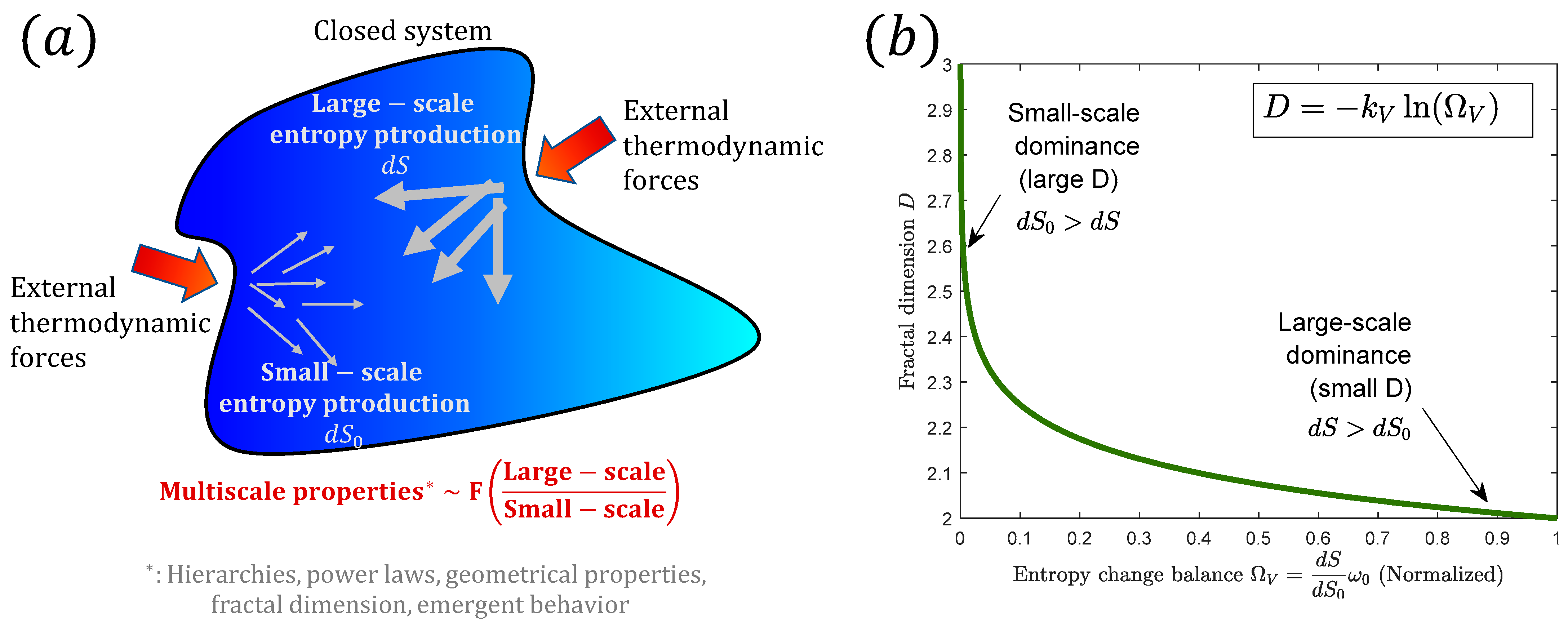
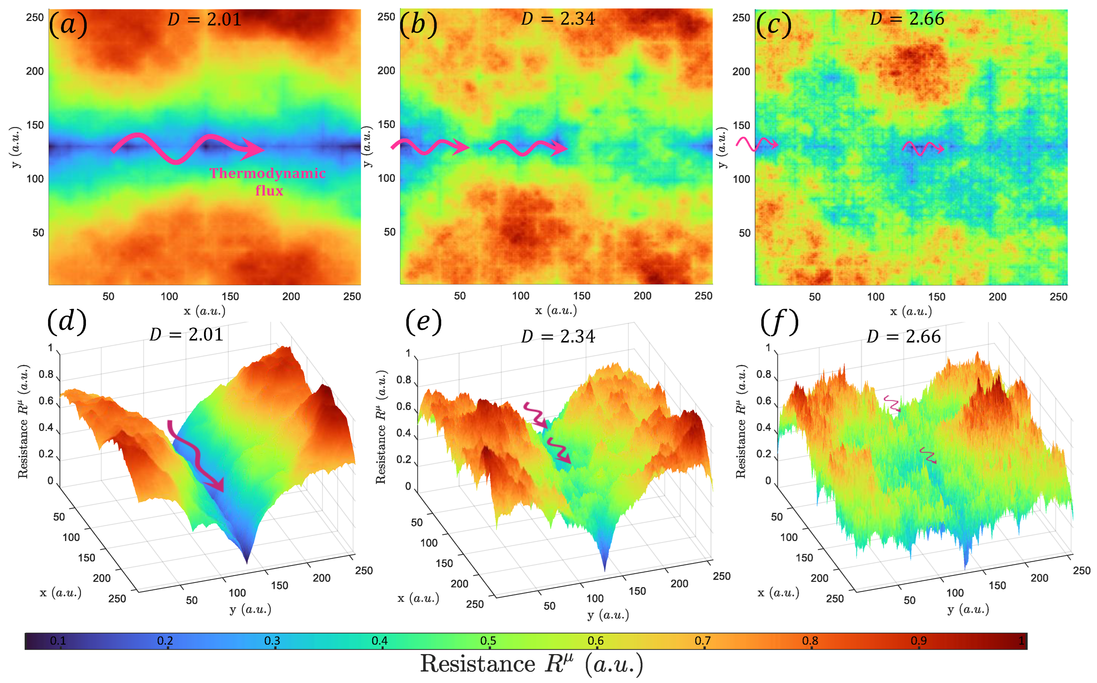
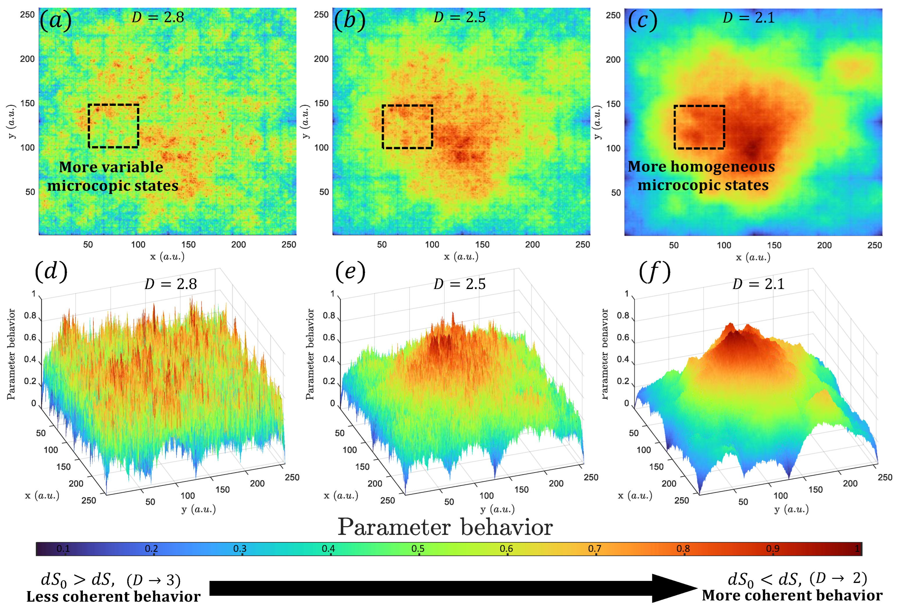
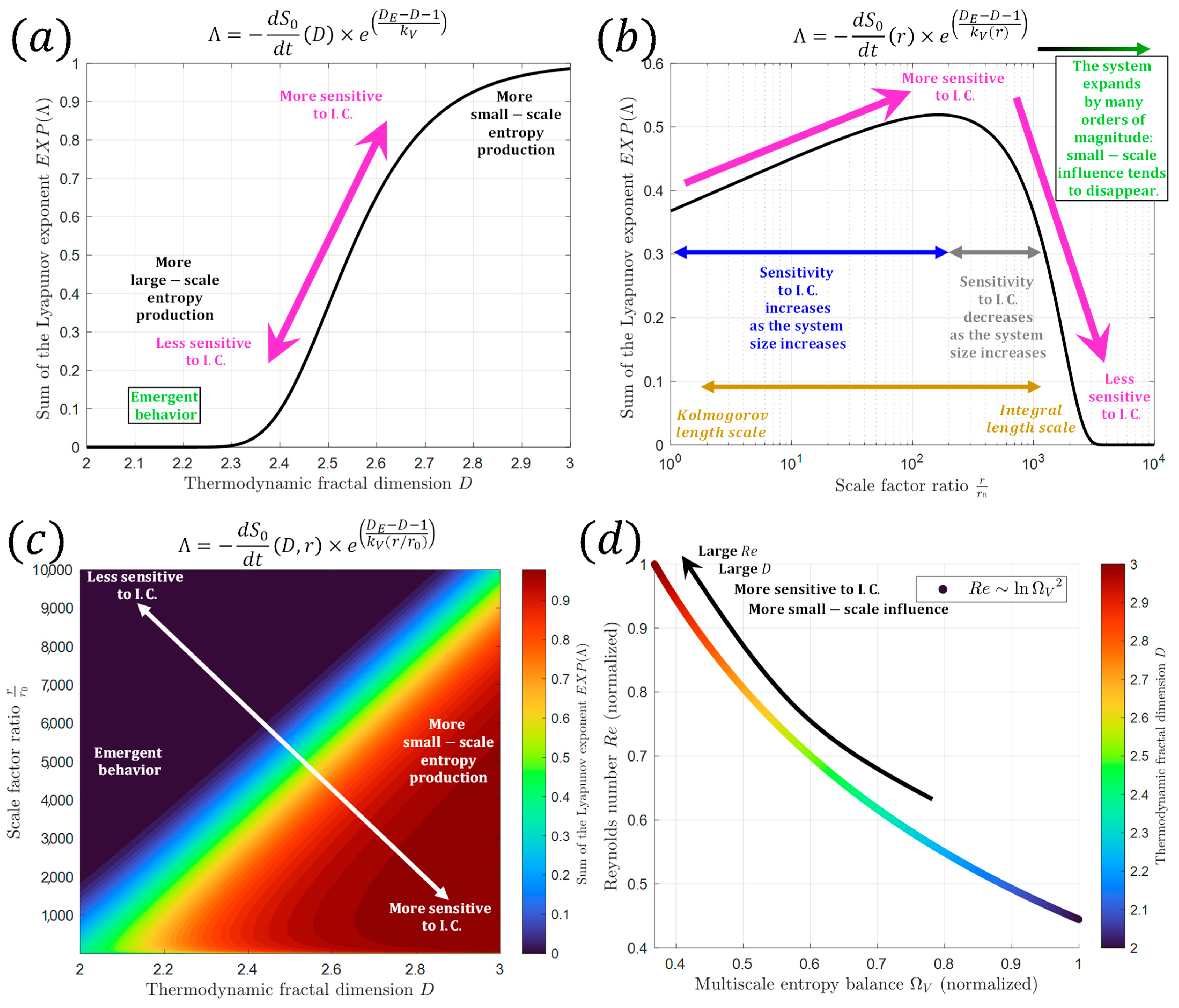
2. The Multiscale Entropy

The concept of entropy is traditionally defined as a macroscopic property that characterizes the degree of disorder or randomness in a system, which is based on the dynamic of large numbers of particles [64,65,66]. However, there have been several attempts to extend this definition to the microscopic level, considering the evolution of individual particles or molecules by using the statistical distribution of the positions and velocities of individual particles, rather than on macroscopic properties such as temperature and pressure [67,68]. Recently, a framework has been developed for understanding how the entropy changes as we move between different scales of observation [53,59]. This view proposes a generalization of Onsager’s reciprocity relations, which relate the transport coefficients of a system to its thermodynamic forces [62,63] by introducing the concept of multiscale resistance coefficients $K_{ij}^{\mu }$, which describe the response of a system to perturbations at different scales. That is [53]:

$$K_{ij}^{\mu }={\left(\frac{r^{\mu }}{r_0}\right)}^{\alpha }{K}_{ij}^{\prime \mu },$$

(1)

where $K_{ij}^{\mu }$ is the local resistance coefficient and $r^{\mu }$ is a scaling parameter, which represents the size or scale of each sub-system, while $\alpha$ is a scaling exponent and $r_0$ is a constant. Here, note that Onsager’s coefficients describe the transport of fluxes and forces that allows systems to be in nonequilibrium. Figure 1a shows a schematic representation of an initially closed system that generates different scales of internal structures due to the external forces. This schematic representation corresponds to the generalization of the observed evolution in the cracking process of rock samples, which occurs due to the application of external loads that generate fractally distributed cracks [53,69,70,71,72,73,74,75,76,77,78]. Thus, this cracking process is regarded as a release of energy that cannot be held in the system due to external inputs. Then, it was considered that this external force could be described by Onsager’s coefficient, which is one of the thermodynamic forces [53]. Here, the thermodynamic fractal dimension $D$ is obtained by the balance between small- and large-scale entropy production, or energy liberation, due to external forces. In other words, $D$ corresponds to the exponent of power laws that rise as a balance between small- and large-scale dissipation of energy when the system cannot hold more external forces. This thermodynamic fractal dimension $D$ is defined as [59]:

$$D=-k_V\ln {\mathsf{\Omega }}_V,$$

(2)

where ${\mathsf{\Omega }}_V$ is the multiscale entropy change balance and is defined as ${\mathsf{\Omega }}_V=\left(\frac{dS}{d{S}_0}\right)e^{\left(\frac{1-D_E}{k_V}\right)}$, $dS$ is the macroscopical entropy change, $d{S}_0$ is the microscopical entropy change, $D_E$ is the Euclidean dimension, and $k_V=1/\ln (r/r_0)$, where $r$ is a scaling factor associated with the size of the largest domain and $r_0$ is a constant that is associated with the dimension of the smallest system. Thus, the thermodynamic fractal dimension (Equation (2)) relates the resistance of a system to the flow of fluxes to the scaling of entropy changes with respect to changes in scale. Therefore, Equation (2) suggests that the fractal properties observed in various physical systems, including the large-scale structure of the universe, may be a consequence of the balance between external forces and the system’s ability to dissipate energy at different scales. Note that the thermodynamic fractal dimension could be negative as Mandelbrot [79] noted. In this case, this occurs when the large-scale dissipation is considerably larger compared to the smallest one. Additionally, it is not additive, so the value of $D$ for a system composed of many subsystems with different values of $D$ does not correspond to the mere sum of their $D$ (see Appendix A).

This multiscale dissipative mechanism could help us to understand the degree of complexity of the system and how it responds to external influences. For example, systems with a higher fractal dimension are more resistant to changes in fluxes because they have a more complex geometrical distribution. This means that these systems are characterized by a greater number of geometric features, such as more irregular surfaces or interfaces. Therefore, the transport of matter, energy, or information in such systems may be hindered, as there are more barriers or pathways to cross [80]. This can result in greater resistance to changes in fluxes or the flow of these quantities in the system. Figure 2 shows the example of the increased relevance of small-scale entropy production by contributing to decreases in the available energy for transport. Note that this figure is created using the algorithm developed by Chen and Yang [81] and Yang [82], which allows for generating fractal surfaces with different smoothness depending on the desired fractal dimension. Also note that in Figure 2, different distributions of thermodynamic resistances are shown, indicating that the opposition to a thermodynamic flow, for example heat, is heterogeneous in space and may vary according to the flow direction. This implies that if the thermodynamic flow encounters a region of higher resistance (red tones in Figure 2), it will generate greater dissipation of energy. In statistical terms, the more complex entropy distribution in a system implies that there are more microstates available to the system. In other words, the more ways there are for the system to arrange its constituents leads to a greater number of microstates and increased entropy [83], which may make the system more resistant to changes. Therefore, systems with higher fractal dimensions may be more stable or robust in the face of perturbations, as they have a greater capacity to distribute and dissipate energy and entropy.

In terms of the multiscale entropy formulation given by Equation (2), a higher thermodynamic fractal dimension means that ${\mathsf{\Omega }}_V$ tends to be small. In other words, the small-scale entropy production $d{S}_0$ is larger than the macroscopical one ($d{S}_0>dS$). That is, in such systems, dissipation occurs primarily at the small scales due to the large number of these irregular features, which leads to a higher degree of entropy production at those scales. In other words, small-scale entropy production can become dominant when there are strong gradients or fluctuations in the system that affect the evolution of individual components or small groups of components, leading to local entropy production that is not reflected in the large-scale evolution of the system. This multiscale dynamic described by Equation (2) is shown in Figure 1b for $k_V=1$ and ${\omega }_0=e^{\left(\frac{1-D_E}{k_V}\right)}=1$.

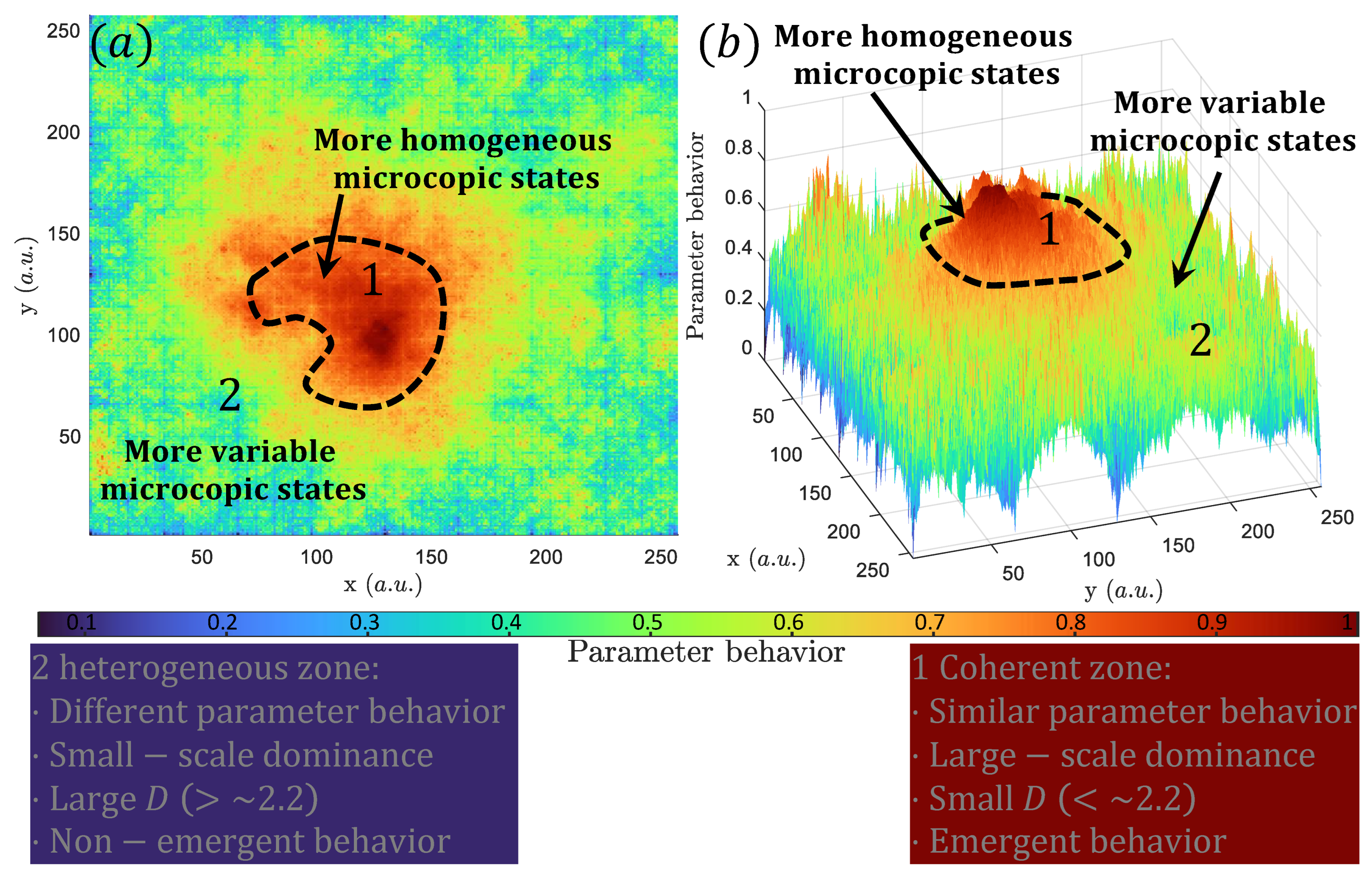
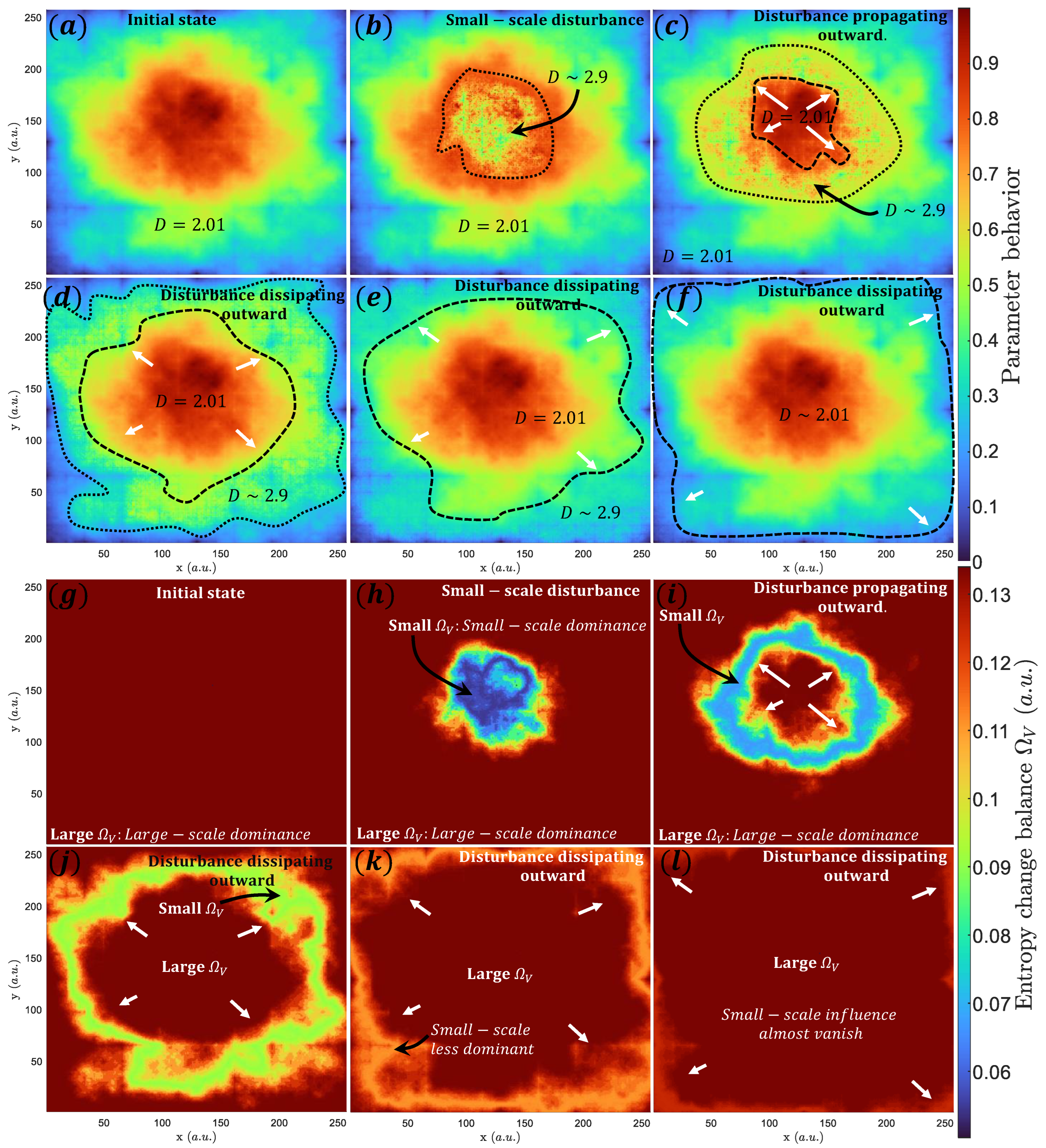
3. On the Emergent Behavior

Equation (2), which is valid for nonequilibrium thermodynamics, also shows that large-scale entropy production is related to the amount of energy that is dissipated by a system at a macroscopic scale. In general, complex systems tend to dissipate more energy at larger scales, resulting in a larger large-scale entropy production ($dS>d{S}_0$). This process is related to the self-organization of the system, which leads to the emergence of new properties and evolutions at different scales [84,85,86,87,88,89,90]. In the context of multiscale thermodynamics, a low thermodynamic fractal dimension implies that the large-scale entropy production is dominant over small-scale entropy production (Equation (2)). This means that energy dissipation occurs over larger spatial scales and is characterized by smooth geometrical properties, indicating that large parts of the system evolve as a unity or exhibit emergent properties. This description is similar to the interpretation of entropy as the unity of system [91]. In such emergent systems, the macroscopic dynamic of the system can be described by a few effective variables or degrees of freedom, and the evolution of the system is relatively simple and predictable. This is because the interactions between the different parts of the system are strongly correlated and the system is described by a low-dimensional attractor (macroscopic patterns or state that the system tends to settle into overtime), which results in the emergence of coherent macroscopic evolution [92,93,94,95,96,97,98]. This description indicates that the large-scale entropy production view is related to the emergence of coherent macroscopic dynamic. This can be seen in the representation that is shown in Figure 3 and Figure 4. Figure 3 shows that large-scale entropy production could produce global coherent behavior. That is, the areas within the black segmented boxes in Figure 3a–c show that different states (represented here as a color palette) are more or less homogeneous depending on the thermodynamic fractal dimension. Large $D$ implies heterogenous states (Figure 3a,d), which are represented by rougher surfaces. Nevertheless, small $D$ indicates that the states within the black segmented box tend to be more homogeneous (represented by smooth surfaces). This is marked as red colors in Figure 3c. Figure 4 shows how a local emergent behavior, similar to that described in Figure 3c,f, can rise in a given area within a system characterized by incoherent states, similar to that described in Figure 3a,d just by changing the thermodynamic fractal dimension. Particularly, Figure 4 is generated by merging Figure 3a,c as $S\left(c\right)=c\times S\left(D=3\right)+\left(c-1\right)\times S(D=2)$ where $S\left(D\right)$ is a fractal surface of fractal dimension $D$ and $c$ is a parameter that is interpreted here as a measurement of the total fractal dimension of the surface $S$. For example, $c=0.8$ implies that $S\left(0.8\right)=0.8\times S\left(D=3\right)+0.2\times S(D=2)$ where the fractal dimension of $S\left(0.8\right)$ is assumed to be $\sim 2.8$ ($D=c+2$) because the geometrical irregularities of $S\left(D=3\right)$ are more dominant than that described by $S\left(D=2\right)$. Thus, the center region of Figure 4 (red colors) is characterized by small values of $c$ and it linearly increases towards the domain boundaries. These examples show that a low thermodynamic fractal dimension is indicative of (in this local) emergent behavior and cooperative dynamics, suggesting that large-scale entropy production could play a key role in producing the observed macroscopic dynamic. However, systems are not always so evident, as fluctuations that reflect a balance between the different scales of the system may exist.

4. The Nature of Fluctuations and Dissipation in Multiscale Systems

Fluctuation–dissipation refers to the relationship between the response of a system to an external perturbation and the fluctuations in the system’s internal state when it relaxes back to equilibrium [99,100,101]. The dynamics in this kind of systems arise as responses to external forces, which is a similar characteristic of multiscale systems. In multiscale thermodynamics, $D$ can fluctuate in space and time due to changes in the multiscale entropy generation, indicating that the system’s entropy production is not constant at different scales. For example, there could be a change in large-scale entropy production that could lead to an increase or decrease in small-scale entropy production, resulting in a change in $D$. This change in $D$ can be considered a fluctuation in the system. In mathematical terms, and by using the definition of ${\mathsf{\Omega }}_V$ given in Equation (2), this can be written as:

$$dS={\mathsf{\Omega }}_V\left(x,t\right)d{S}_0{e}^{\left(\frac{D_E-1}{k_V}\right)}.$$

(3)

Equation (3) indicates that the large-scale entropy change $dS$ influences the small-scale entropy change $d{S}_0$, and vice versa, by means of a multiscale balance term ${\mathsf{\Omega }}_V(x,t)$. Thus, ${\mathsf{\Omega }}_V$ can be regarded as a function that transfers perturbations across different scales because it determines how dissipations occurs at multiples scales. Therefore, changes in the multiscale balance term ${\mathsf{\Omega }}_V$ can cause the thermodynamic fractal dimension to change, which means that the system can exhibit multifractal dynamics and the system’s evolution could become even more complex. Thus, $D$ can be used to describe the fluctuation-dissipation properties of the system.

Let us consider a perturbation that increases $D$ at the center of a system characterized by small $D$ values. As the perturbation spreads outward, the dissipation of energy associated with these fluctuations can be described by the fluctuation–dissipation theorem. In this case, as the perturbation spreads outward and the thermodynamic fractal dimension increases, the system is expected to respond with larger fluctuations. The fluctuation–dissipation theorem then predicts that the dissipation of energy associated with these fluctuations will also increase. However, as the perturbation decreases, the thermodynamic fractal dimension will eventually reach a steady state, at which point the fluctuations and dissipation will stabilize. This scenario can be seen in Figure 5 where the system $S$ is characterized by a single thermodynamic fractal dimension $D=c+2$, which can be described using the same relation used in Figure 4. In this case, the factor $c$ is not linear but Gaussian and is defined as $c=\left(1-c_0\right)\times \exp \left(-c_1{\left(c_i-c_0\right)}^2\right)$, where $c_0$ and $c_1$ are constant and $c_i$ is spatial variable. Thus, the state of the system can evolve more macroscopically or microscopically depending on $c$. This means that $c=0$ implies that $S=S\left(2\right)$ and the system will act more macroscopically because the spatial variation of states is small. In contrast, $c=1$ implies that $S=S\left(3\right),$ which generates large spatial variation among different parts of the system. The factor $c_0$ determines where the maximum $c$ is found. In other words, if $c_0$ is moving from the center of the system to its boundaries, it implies that the microscopical dynamic is spreading from the center outward. This can be seen in Figure 5a–f. Particularly, Figure 5a shows a system characterized by a large-scale influence, which implies that the spatial variations of its states (color palette) are smooth. Figure 5b–f reveals the propagation of a disturbance that generates an increase in $D$ (area within the segmented black lines). The white arrows indicate the direction of the disturbance front. The multiscale entropy balance can be expressed using Equation (2) as:

$${\mathsf{\Omega }}_V=e^{-\frac{D}{k_V}}=e^{-\left(c+2\right)}.$$

(4)

The spatial distribution of ${\mathsf{\Omega }}_V$ can be obtained. Figure 5g–l shows the spatial evolution of Equation (4) for $k_V=1$. Initially, ${\mathsf{\Omega }}_V$ is completely dominated by a large-scale entropy change (red shades in Figure 5g). As the small-scale influence increases (blue shades in Figure 5h), it also propagates outward (Figure 5i–l). In addition, the small-scale influence also tends to decrease as it propagates to the domain’s boundaries. This can be seen as blue to light red shades in Figure 5j–l. Thus, this example has shown how the spatial and temporal changes in ${\mathsf{\Omega }}_V$ can represent the multiscale fluctuation and dissipation within a system.

The contribution of entropy production at different scales, defined by the multiscale balance term ${\mathsf{\Omega }}_V(x,t)$, could also be used for other diffusive system such as those that incorporate chemical reactions. For example, biological morphogenesis, which corresponds to the process that could generate observable macroscopical patterns in animals, has been regarded because of the interaction between diffusion and reaction processes [102]. As the gradient of chemical potential and chemical reactions can be related to Onsager’s coefficients [103,104], it is expected that ${\mathsf{\Omega }}_V(x,t)$ could be useful in characterizing the efficiency of the dissipation of energy at different scales and how it contributes to the emergence of Turing patterns, particularly because many of these interactions and dissipation within a system can form patterns or structures where some features can be distributed as power laws [105,106,107,108,109,110], which suggests that the physics of pattern formation may be directly associated with the principle of multiscale dissipation. However, more research is needed to fully explore this potential connection.

4.1. Temperature and Critical Phenomena in Biological Systems

Critical phenomena refer to the evolution exhibited by physical systems near a critical point or phase transition [111,112,113,114,115]. A critical point represents the boundary between different phases of a system, such as the transition from a liquid phase to a gas phase [116,117]. Near the critical point, these properties exhibit power law scaling, with critical exponents characterizing the rate at which they change [118]. In terms of temperature, the critical temperature defines the temperature at which a phase transition occurs. When there is an increase in temperature, the particles in a substance gain kinetic energy, resulting in increased movement at the microscopic scale and an enhanced heat capacity [119]. This increased movement enables the system to disperse and distribute the energy input across smaller scales. That is, the small-scale entropy production ($d{S}_0$) must increase, which leads to increases in the thermodynamic fractal dimension (Equation (2)) in terms of the increase in temperature. This type of evolution can be observed in some biological systems. For instance, the critical exponent $\beta$, which describes the exchange of ions and charges at the cellular level across multiple scales, tends to increase as the system approaches the critical temperature [120]. Consequently, the macroscopic entropy decreases near the critical temperature [121]. In this regard, the principles of multiscale thermodynamics offer a physical interpretation of this phenomenon because $\beta$ could be directly related to the thermodynamic fractal dimension. This suggests that the system seeks to dissipate energy at the microscopic level rather than at the macroscopic level, resulting in a reduction in macroscopic entropy. This implies that the increase in temperature has a microscopic effect that is relevant to understanding biological processes. For example, this effect is particularly important for the regulation of homeostasis, which will be discussed in Section 7.7. It is also important to add that $D$ is associated with changes in dissipation and not directly with temperature. This means that if there is a system in which the temperature decreases, $d{S}_0$ will also decrease, which could cause $D$ to tend toward zero. However, this description is only true if there are no macroscopic changes. Thus, the value of $D$ will depend on how the system dissipates energy macroscopically. This has implications for reaching absolute zero. For example, a lower temperature implies that $d{S}_0$ must tend to zero, which could cause both ${\mathsf{\Omega }}_V$ and $D$ to diverge. This suggests that one way to achieve this goal is to reduce macroscopic dissipation.

5. Chaos Theory

The relationship between the thermodynamic fractal dimension and chaos theory lies in their shared focus on understanding and describing complex systems and the use of mathematical tools to characterize these dynamics. Particularly, the relationship between chaos theory and power laws arises from the concept of fractal dimension [122]. Fractals are objects or patterns that repeat at different scales, and they are often characterized by power law scaling relationships [60] and self-organization [123,124]. Power laws are closely related to the concept of self-similarity, which is a key characteristic of fractals [125]. In contrast, chaos theory deals with the evolution of dynamic systems that are highly sensitive to initial conditions [126]. This sensitivity and the degree of chaos in the system can be described by the sum of the Lyapunov exponent spectra $\mathsf{\Lambda }={\sum }_j{\lambda }_j$ where ${\lambda }_j$ is the $j$th Lyapunov exponent. Thus, a more positive ${\lambda }_j$ suggests more chaotic and unpredictable outputs [127,128,129]. Therefore, to understand the relationship between multiscale entropy production, chaos theory, and sensitivity to initial conditions, it is necessary to analyze the Lyapunov exponent spectra and their relation to the entropy production. A simple relation between entropy production and the Lyapunov exponent spectra is known as the Nose–Hoover relation [130,131,132]:

$$\frac{dS}{dt}=-\mathsf{\Lambda }>0.$$

(5)

Here, this entropy production represents the global macroscopical system and the negative sign represents the irreversibility. This indicates that in a chaotic system, where at least one positive Lyapunov exponent exists, the total sum of $\mathsf{\Lambda }$ should be negative. When the time is reversed, $\mathsf{\Lambda }$ is positive, which implies that the possible trajectories are more unstable, which prevent it from recovering the initial state [130]. Here, positive (negative) $\mathsf{\Lambda }$ means that there are more positive (negative) Lyapunov exponents, and/or the positive (negative) exponents that already exist are larger. In this regard, it could be interpreted that larger positive $\mathsf{\Lambda }$ could represent a more “chaotic system”. By using Equations (3) and (4) in Equation (5), the Lyapunov spectrum can be related to the thermodynamic fractal dimension as:

$$\mathsf{\Lambda }=-\frac{d{S}_0}{dt}{e}^{\left(\frac{D_E-D-1}{k_V}\right)}.$$

(6)

Note that, here, the maximum positive $\mathsf{\Lambda }$ could not necessarily be related to $\mathsf{\Lambda }$. Equation (6) shows that there is a direct relationship between the sum of Lyapunov exponents and the thermodynamic fractal dimension, where a smaller $D$ is associated with smaller values of the sum of Lyapunov exponents. This can be seen in Figure 6a where $D_E=3$, $d{S}_0/dt=dS/dt \mathrm{e}\mathrm{x}\mathrm{p}(\left(D+1-D_E\right)/k_V)$ and $dS/dt=1 (a.u.)$, where a.u. stands for arbitrary units. Equation (6) and Figure 6a also show that smaller $D$ values are associated with smaller values of $\mathsf{\Lambda }$, implying that emergent behavior could be related to systems that are not too sensitive to initial conditions. Figure 6b shows that the relationship between $\mathsf{\Lambda }$ and the scale of the system $r$ is not linear. At small scales, the sum of Lyapunov exponents increases as the scale increases, indicating that the system becomes more chaotic and sensitive to initial conditions. However, at larger scales, the sum of Lyapunov exponents starts to decrease, indicating that the sensitivity to initial conditions becomes less relevant as the system expands to different scales. This suggests that the emergent behavior of a system may be limited to a specific range of scales, beyond which the influence of small-scale conditions becomes negligible. Figure 6c shows the combined effect of $D$ and $r$.

6. Turbulence

Turbulence is a type of fluid flow characterized by irregular and chaotic fluctuations in velocity and pressure. These fluctuations occur over a wide range of spatial and temporal scales, making turbulence a multiscale phenomenon. This means that turbulent flows often exhibit power law scaling in their statistical properties, such as velocity fluctuations [133]. Particularly, turbulence occurs in fluid flows at high Reynolds numbers and is characterized by the presence of small-scale vortices and eddies that interact with each other in a nonlinear way [134]. According to Nicolleau [135], the fractal dimension of the fluid can be linked to the Reynolds number $Re$ as:

$$D\sim {\left(Re\right)}^{\frac{1}{2}}.$$

(7)

By considering Equations (2) and (7), the Reynolds number can be written as:

$$Re\sim {\left(\ln {\mathsf{\Omega }}_V\right)}^2.$$

(8)

Equations (2) and (8) can be useful tools for characterizing turbulence because it captures the multiscale nature of the flow. In particular, a high $D$ could be associated with turbulence because it indicates that the small-scale fluctuations in the flow are dominant. This implies that the Reynolds number is also large (Equation (8)). This can be seen in Figure 6d. Another relation between multiscale thermodynamics and turbulence is the scale restriction shown in Equation (6) and Figure 6b. This scale restriction suggests that the influence of small-scale features on the overall dynamic of the flow is limited to a certain range of scales, beyond which their effect becomes negligible. This is consistent with the idea that turbulence is a phenomenon that is only present within a certain range of scales, and that its effect on the overall evolution of the flow diminishes as the scale of the flow increases [136]. For example, the Kolmogorov length scale represents the smallest length scale at which turbulent energy dissipates into heat due to viscous effects and it is typically several orders of magnitude smaller than the integral scale, which represents the largest-length scale of energy-containing eddies in turbulent flow [137]. In terms of initial conditions, a small difference in the initial conditions of the Kolmogorov length scale can be amplified as the fluid flows and becomes more turbulent. This can lead to significant differences in the dynamic of the flow at larger scales, including the integral scale [138,139,140,141]. In other words, small-scale fluctuations at the Kolmogorov length scale can cascade up to larger scales, affecting the flow at those scales. This phenomenon is known as the (inverse) “cascade of energy” in turbulent flow.

The scale-restriction shown in Equation (6) and Figure 6b suggests that the effect of small-scale disturbances on larger scales is limited. This is because the larger scales are less sensitive to small-scale disturbances, which is similar to the idea that a small difference in initial conditions of the Kolmogorov length will not significantly affect the fluid at the scale where the integral turbulence scale is defined. In both cases, the effect of small-scale disturbances is limited to a certain range of scales. Thus, turbulent systems can be seen as an example of this scale restriction (Equation (6)).

7. Other Examples

The universe is composed of systems that go beyond the most basic physical sciences, so this section is dedicated to presenting several examples of multiscale processes present in different systems, such as geophysics, astrophysics, biology, and the social sciences, which could be linked to multiscale dissipation processes. This is because these systems encompass a wide range of scales, from the atomic level to the scale of the universe, and often involve interactions between different scales. The examples presented in this section seek to understand the applicability of Equation (2) in various fields of science.

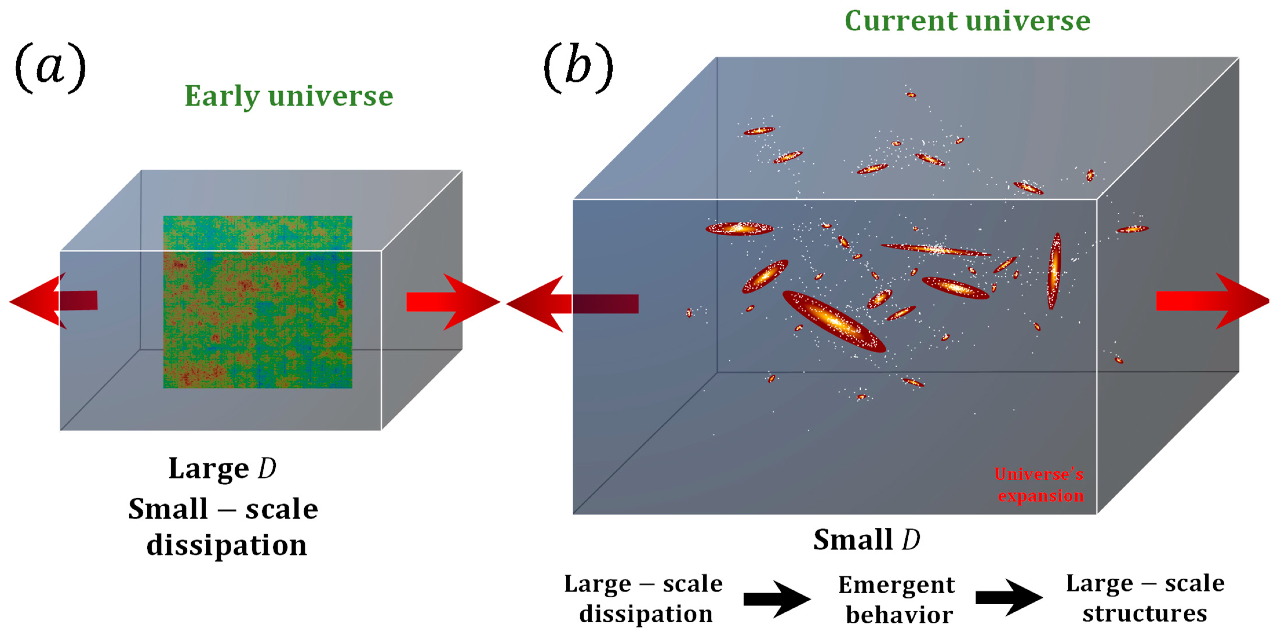
7.1. Complexity and Cosmic Evolution

According to Chaisson [142], the complexity of the universe has been increasing over time because it creates emergent structures, such as galaxies and clusters of galaxies, which are formed by interactions between smaller structures. Chaisson’s perspective is based on the idea that the complexity of the universe is directly related to the ability of matter to store energy per unit volume. He suggests that as new structures are formed throughout cosmic evolution in an expanding universe, they become more efficient at storing energy. As these structures in the universe are commonly multiscale systems governed by power laws [143,144,145,146,147,148,149,150,151,152,153,154], it is worth analyzing Chaisson’s view of complexity in the context of the multiscale phenomenon described by Equation (2). Particularly, some scientists consider that some physical concepts, such as entropy production, should be excluded from the description of the universe’s complexity due its lack of strict meaning, which generates misconceptions outside physical sciences [91,155,156,157,158].

While some aspects of complexity can be captured by power law distributions, the key aspect is the interpretation associated with the expanding universe. To date, there is no interpretation of the origin of this expansion, which allows us to consider that it could also have an external origin. This would mean that the universe itself could be considered an open system, which is the foundation of the multiscale thermodynamics perspective. This would therefore indicate that the universe itself could be described or characterized by a “universal” or large-scale value of $D$. In fact, this is observed on a large scale when looking at large structures from the past. For instance, studies have found evidence suggesting that at the beginning of the universe, the structures were characterized by a large fractal dimension (equivalent to $D>2.6$ in the two-dimension representation) [152,159,160]. In contrast, the large-scale galaxy distributions that we observe today are characterized by a fractal dimension that is lower than that of the early universe ($D<2.6$) [161]. In the context of the multiscale thermodynamic fractal dimension, this suggests that the early universe was more efficient at dissipating energy at smaller scales. Equivalently, the early universe was dominated by low (microscopic) entropy [162]. Then, the universe became more efficient at dissipating energy at larger scales over time, which led to the emergence of large-scale structures such as galaxy clusters and superclusters. This can be seen schematically in Figure 7, which shows the evolution of the universe’s thermodynamic fractal dimension and how it is related to the emergence of large-scale structures over time. Thus, as the universe continues to expand, we may expect to see further evidence of this kind of emergent behavior and the development of larger and more complex structures and patterns. In other words, this is in line with the idea that the expansion of the universe is one of the factors that contribute to the increasing complexity of the universe through emergent behaviors. The ability of a system to self-organize and self-maintain its own organization, such as homeostasis or autopoiesis [163,164,165,166], could be a consequence of the decreases in the thermodynamic fractal dimension of the universe. This contradicts the idea that there were some large-scale structures in the early universe, unless these structures were remnants of a prior large-scale universe [167,168,169,170]. Note that in this context, the fact that a system is more efficient at storing energy per unit mass could be interpreted as meaning that this storage is actually a useful means of generating dissipation at a larger scale.

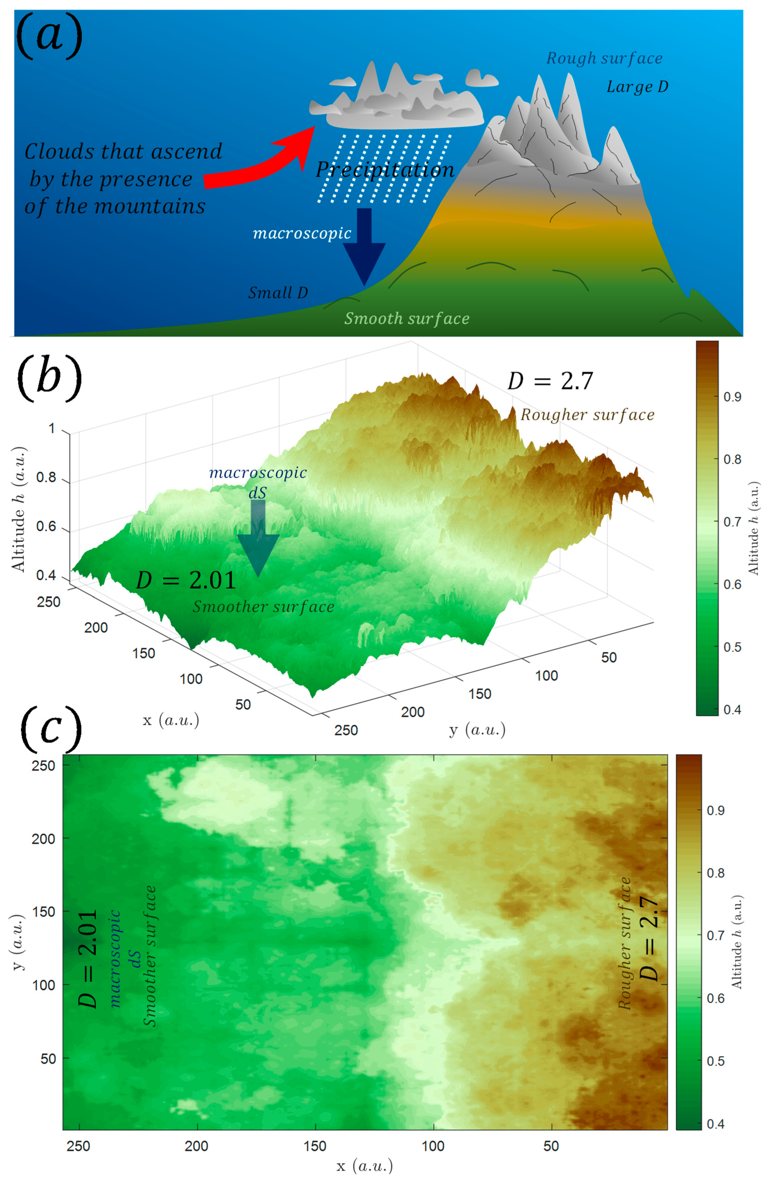
7.2. Mountain Range Geomorphology

Jumping to a more human perspective, our experience is linked to the topography of the places we inhabit, which have different roughnesses. In particular, geometrical properties of geological structures have commonly been described as power law [60,171,172,173,174,175]. That is why $D$ could also be related to geological features. In this multiscale context, the generation of topography can be understood as the result of the balance between macroscopic and microscopic forces that act on the Earth’s surface. For example, if energy is dissipated primarily at small scales, this can lead to a rough and jagged landscape. However, if energy is dissipated more efficiently at larger scales, this can lead to smoother and more regular topography at larger scales. The relationship between energy dissipation and topography can also be influenced by external factors such as climate and atmospheric conditions, indicating that topography is an open system. For example, mountains can affect rain conditions because it can block the movement of clouds, which enhance precipitations [176]. As precipitation can generate smooth surfaces [177] by causing the erosion of the most pronounced geometric roughnesses, the generation of topographic smooth surfaces due to climate can be regarded as a macroscopical force. Figure 8a illustrates the relationship between the thermodynamic fractal dimension and the topography of a mountain range. The obstruction of cloud movement by the mountain generates macroscopic dissipation and reduces the thermodynamic fractal dimension, creating smoother surfaces at the bottom or piedmont regions. Figure 8b,c show two views of a random multifractal distribution with a fractal dimension of 2.01 at the bottom and 2.7 at the peak. The decrease in altitude is characterized by smaller values of D, which generates a topography similar to that found in real mountain ranges.

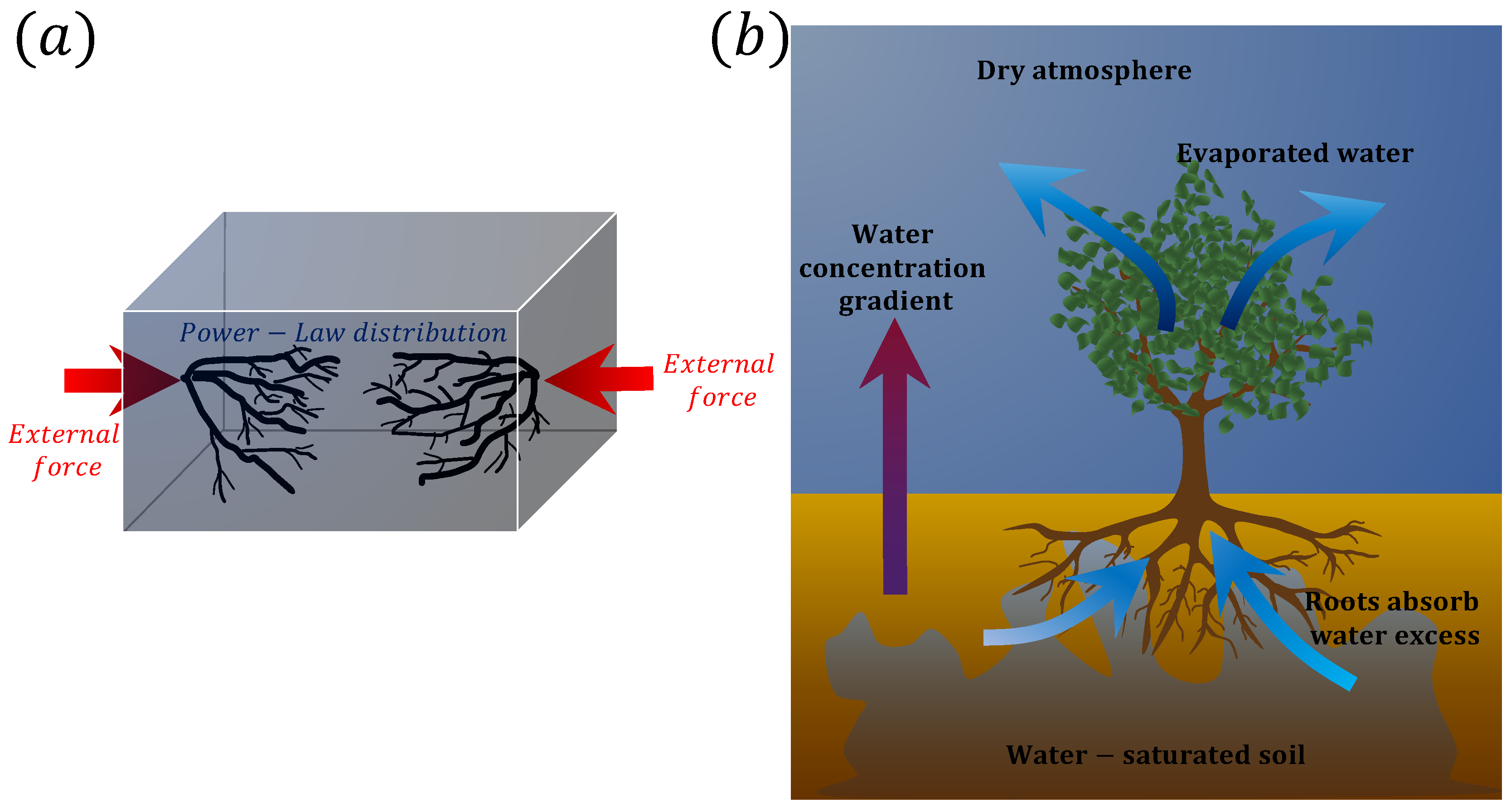
7.3. Tree’s Transpiration Process and Life System Governed by Power Laws

Some systems that follow power laws ordering are those that exhibit “branching” properties as a result of efficient matter transport. For example, the branching of a tree and plants can follow a self-similar pattern where each branch bifurcates into two, or more, smaller branches, and this pattern repeats at different scales within the tree [29,178]. This can be described using a power law relationship between the diameter or length of a branch and its position within the tree, while the distribution of leaves or needles on a tree can also exhibit fractal patterns, where the distribution is self-similar at different scales [29,179]. These features, along with the tree-shaped design found in nature, allow for efficient transport of fluids or mass from volume/area to point, as facilitated by the pressure generated by the concentration gradient of water from moisture-saturated soil to the dry air [180]. This gradient of water potential between the soil and the atmosphere, which drives the flow of water from the roots to the leaves, is known as transpiration [181,182]. The transpiration process of trees can be seen as an example of an irreversible process in a multiscale system, where external forces generate power laws. In this case, the external force is the gradient concentration of water between the soil and the atmosphere, and the power law arises as a result of the efficient transport of fluids from the water-saturated soil to the dry air through fractal and self-similar structures (roots and branches) [180,183]. As shown in Figure 9, the patterns that form in trees, initially considered a consequence of efficient water transport, can now be viewed as a form of entropy generation across multiple scales. In this context, the design of trees, which arises as a consequence of efficient water transport as described by Bejan [183], can now be seen as a manifestation of a universe striving to evolve toward a more probable state. This process is inherently irreversible, and trees operate under the same principle within this multiscale framework. In other words, this suggests that the fundamental characteristics of a tree, such as its power law scaling, irreversibility, and being affected by external forces, are consistent with the ideas of multiscale thermodynamics.

As several systems in biology are governed by power laws [184,185,186,187,188,189,190], it is possible that some systems in life science are irreversible due to the basic properties of multiscale thermodynamics proposed in this work. This would suggest that open biological systems described by power laws, such as tree branching, circulatory and respiratory systems, or even the body size distribution in ecological communities, could be local manifestations of the dissipation of energy at multiple scales [191,192,193,194,195,196]. These systems are constantly interacting with their environment and exchanging energy and matter, and thus, are subject to external forces that drive irreversible processes [197]. Thus, the study of multiscale thermodynamics provides a framework to understand the emergence of power laws and irreversibility in complex biological systems.

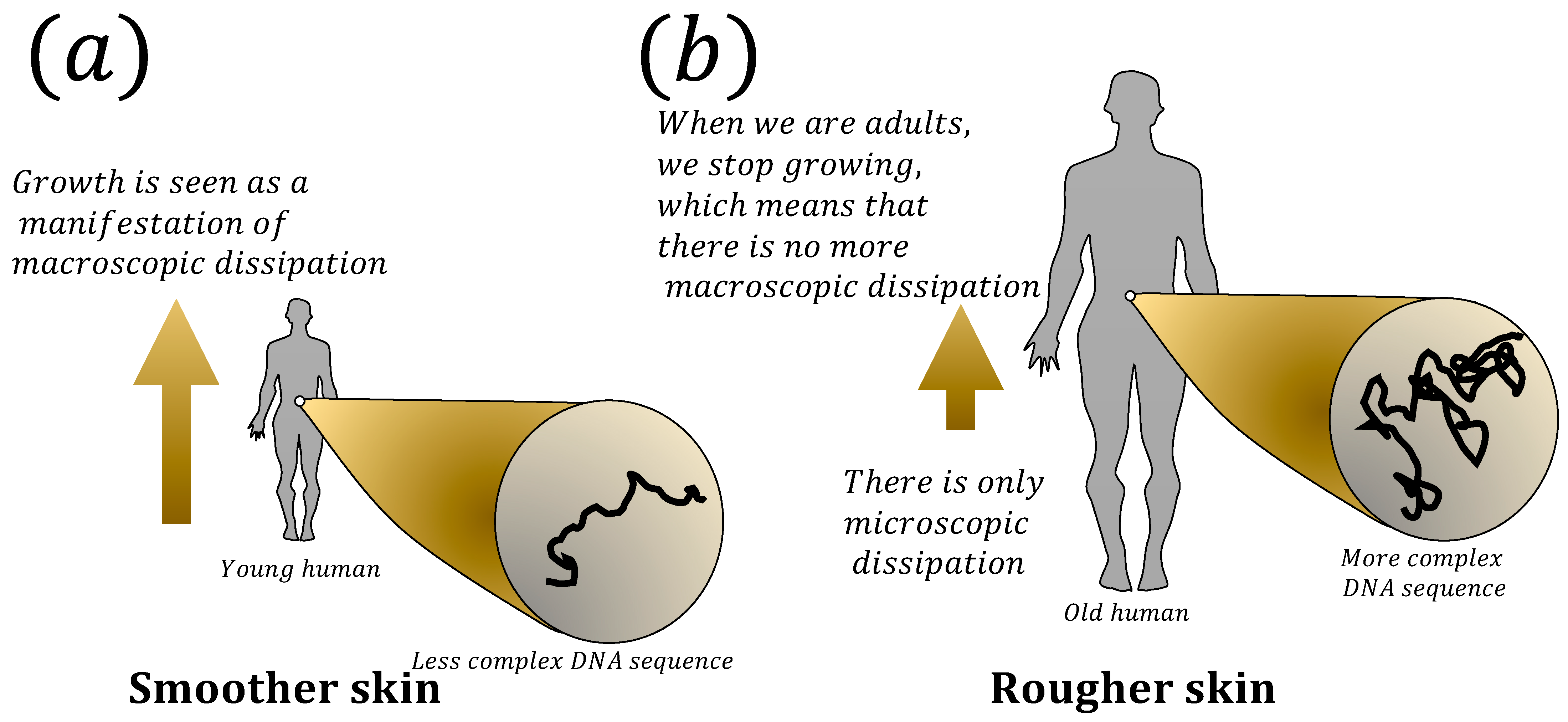
7.4. Geometry of Human Organs and Aging

As described in Section 7.3, human organs could also exhibit power law and fractal characteristics in their structure and function. For example, the bronchial tree and air sacs in the lungs exhibit a fractal branching pattern that maximizes the surface area available for gas exchange, the blood vessels within the heart exhibit a fractal-like branching pattern that allows for the efficient delivery of oxygen and nutrients to the cardiac tissue, and the dynamics of neural activity also exhibit power law scaling reflecting the complex interactions among neurons [198,199,200,201,202]. That is why the relationship between human organs and power law can be understood in the context of multiscale thermodynamics. In the case of human organs, external forces could be related to the demands of the body for a particular function or the constraints imposed by the physical environment. These external forces create a need for the efficient transport of nutrients, oxygen, and waste products across various scales, ranging from the microscopic capillary networks to the larger vessels and ducts. The fractal organization of human organs, such as the lungs or the circulatory system, can be seen as a response to these external forces, as it allows for the optimal exchange of materials while minimizing the energy required for transportation [9,180]. The fractal organization of human organs can also be seen as an example of how nature utilizes the principles of multiscale thermodynamics to optimize energy consumption and dissipation. In other words, what is interpreted as efficient transport could actually also be interpreted as an efficient form of energy dissipation. Similarly, the increase in the fractal dimension of DNA walks, which refers to the spatial arrangement of the DNA double helix, and human faces during aging [203,204,205] could be manifestations of the same principles, as the system seeks to dissipate energy in a more efficient manner at smaller scales. For instance, Namazi et al. [205] found that both the fractal dimension of DNA walk and skin rugosity increase with age. Similar findings are obtained in other organs, such as the lung, indicating that the respiration process becomes more complex as we age [206]. This increase in the thermodynamic fractal dimension could be excessive for some organs because this may indicate the presence of intense small-scale dynamics that could lead to tumor proliferation. In fact, the increase in the fractal dimension of tissues is a characteristic of organs affected by cancer, while successful treatment is reflected in a decrease in the fractal dimension [207,208]. This suggests that the human body, including some diseases, can be described as a whole by $D$. This could be more evident for aging. For example, this perspective suggests that growth could be a macroscopic manifestation of biological forces that dissipate energy. According to the multiscale thermodynamic view, macroscopic dissipation results in smaller thermodynamic fractal dimensions and smoother surfaces, which explains why young humans have smooth skin and less complex DNA sequences. However, as humans age and stop growing, the body cannot dissipate energy at a macroscopic scale, leading to more relevant microscopic dissipation. This results in more complex DNA sequences and greater skin rugosity. This process is schematically described in Figure 10.

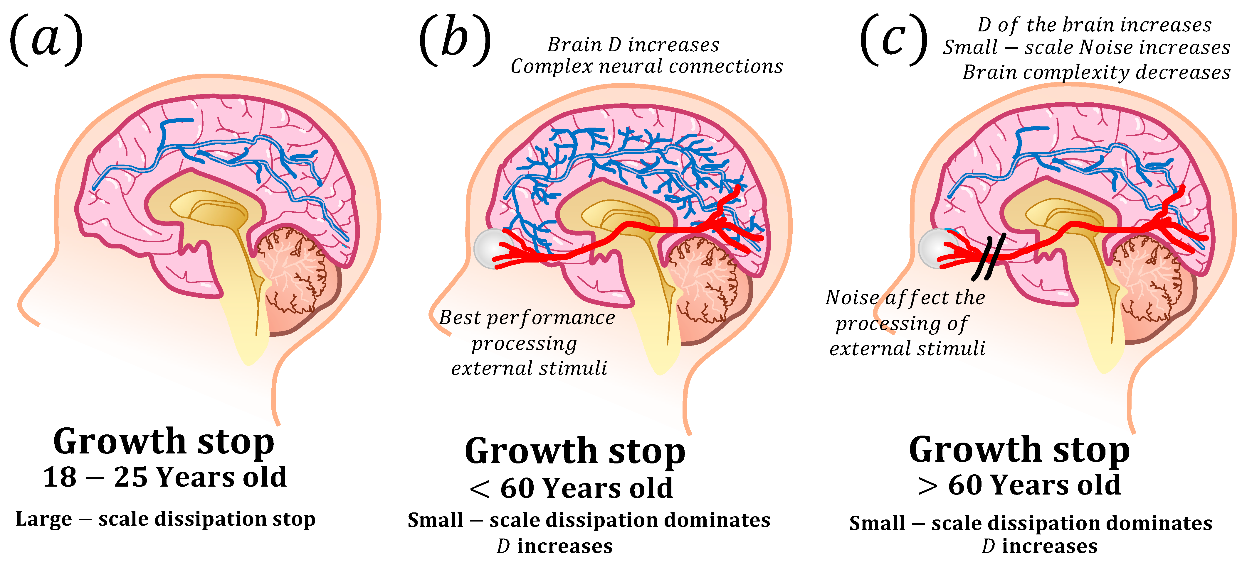
7.5. Human Brain and Cognition

One of the most interesting organs in the human body is the brain. The brain has a complex structure that can be described using power laws and fractals [209,210]. This means that the structure of the brain is self-similar at different scales and can be characterized by a fractal dimension. The fractal dimension of the brain has been found to be a relevant parameter related to cognition [211]. In other words, the more complex the structure of the brain, the larger the fractal dimension and the better it performs cognitive tasks. This is because a more complex brain structure can support more complex neural connections and information processing [212,213]. It is relevant to highlight that the complexity of the brain, as measured by its fractal dimension, is not constant as we age. Research has shown that the fractal dimension, and thus the network complexity of the brain, tends to increase from young adulthood (<40 years old) to mid-age (40 to 60 years old) and then decrease from mid-age to old age (>60 years old) [214,215,216]. The latter is due to the gradual degradation of neural connections and the loss of brain tissue, which suggests that age-related changes in brain structure contribute to cognitive decline. External stimuli, such as sensory information from organs like the eyes and skin, can increase the fractal dimension of the brain [217]. This is because external stimuli influence the brain to create new neural connections and processes information in a more complex way [98]. That is, our episodic memory (remembering specific events) and semantic memory (meaning of the world) are also ways to map the state of neural connections given the interaction with the environment [218,219]. Therefore, activities that involve exposure to new sensory information, such as learning a new language or playing a new instrument, can lead to an increase in brain complexity and improved cognitive function [220]. This implies that external stimuli could rewire brain networks in elderly people [221]. The multiscale thermodynamic framework described by Equation (2) suggests that human growth is related to large-scale dissipation (Section 7.4), which occurs during childhood and adolescence. In adulthood, when large-scale dissipation stops, there is a burst of small-scale dissipation that could increase the fractal dimension of the brain’s neural networks. This can be seen as increases in the fractal dimension, white matter, and cognitive abilities in young adulthood [222]. Organs, such as the eyes and skin, are at their best performance during this period and provide a steady stream of external stimuli that can drive this small-scale dissipation generating increases in the brain’s fractal dimension. Figure 11a,b show a schematic representation of the increases in the thermodynamic fractal dimension at theses ages. Nevertheless, small-scale dissipation could also generate fractal noise, which affects cognition in elderly people [223,224,225]. However, as the aging process progresses, the channels that connect the brain to the external world may vanish due to the degradation of organs such as the eyes [226]. Besides the increasing brain noise, this can lead to a lack of external stimuli, which in turn generates less small-scale dissipation and lower fractal dimension values. This decline in the fractal dimension could lead to a reduction in plasticity, cognitive abilities, and neural connections. Thus, it can be said that the power law structure of the brain is a consequence of external forces (stimuli), and its efficiency is driven by both the small-scale entropy production due to the stop of macroscopical growth and the degradation of channels that connect the brain and the external world. In other words, the changes that the human brain could experience throughout its development could be strongly influenced by processes similar to those described by multiscale thermodynamics. Key characteristics such as the influence of external forces (stimuli) and the power law distribution (directly associated with cognitive abilities and the fractal dimension) suggest that the brain is another example of the application of multiscale thermodynamics. Note here that this view would imply that the brain, like the rest of the organs described, is dissipative in nature, so its ability to map, understand, or interact with the world could be a secondary process or consequence of dissipation.

7.6. Evolutionary Moral

The brain’s structure and function are essential for modeling or influencing the complex social behavior of mammals. In particular, complex systems theory can be applied to study the emergence of social norms, which are unwritten rules of behavior that are enforced through social pressure rather than legal sanctions [227,228,229,230]. Social norms can arise through complex interactions between individuals, as people observe and mimic the behavior of others, and can be reinforced or weakened through feedback loops [231]. According to Tomasello [231], the capacity for shared intentionality allows humans to engage in collaborative activities, such as hunting, gathering, and child-rearing, which require individuals to work together and coordinate their actions towards a common goal. This implies that the emergence of morality can give rise to new actions and social structures that are not reducible to the behavior of individual components. Particularly because morality emerges from the interactions and relationships between individuals, it is sustained by social norms, institutions, and practices that are created and maintained by the group. In other words, once cooperation and shared goals become established, they tend to persist and become increasingly complex. This indicates that social norms arise from the interaction between people or groups, as well as with the environment. This also suggests that there is an external force that models human behavior. Nevertheless, the consideration of power laws to explain social interactions may be more diffuse. That is why human morality may be more difficult to identify as a consequence of multiscale thermodynamics. This implies that the concept of emergent behavior [232] is required to link human behavior with multiscale thermodynamics in an indirect manner.

For example, Section 3 suggests that the small values of $D$ indicate that the system acts similarly across different scales, generating macroscopic patterns that persist over time because they are difficult to erase. Therefore, it is possible to interpret the emergence of shared intentionality in human morality as a result of the interactions of individuals in social contexts, similar to how emergent behavior and macroscopic patterns can arise in complex systems through the interactions of individual components at smaller scales. In that line, the moral norms, values, or “union feelings” that make people gather (such as ideologies, nationalism, religions, sports teams’ supporters, or patriotism) that emerge in a society that are likely to persist over time (difficult to reverse or undo) could be seen as consequence of the multiscale thermodynamic framework.

7.7. Updating the Perspective of Natural Selection and Biological Death

The evolutionary changes that groups of living beings undergo over long periods of time can make it easier or harder for their members to survive. This is described by natural selection, which is one of the most fundamental principles in evolutionary biology [233]. It states that in a population, individuals with traits that are better adapted to their environment are more likely to survive and reproduce, passing on these advantageous traits to their offspring [234]. Over time, this process leads to changes in the traits of a population, ultimately resulting in the “adaptation” of organisms to their environment. When the multiscale thermodynamic phenomenon is considered, the principles of natural selection undergo an interesting reinterpretation. In traditional Darwinian theory, adaptation is primarily driven by the need to survive and reproduce in a given environment. However, from the multiscale thermodynamic viewpoint, the focus shifts towards the dissipation of energy and the increase in macroscopic entropy, which is a feature of cosmic evolution.

In this context, as the universe reduces its thermodynamic fractal dimension (Section 7.1), it implies that systems tend to dissipate energy more efficiently on a macroscopic scale, leading to emergent behaviors (Section 3). In other words, particles may tend to exhibit similar dynamic, which gives rise to the creation of larger coordinated structures, such as multicellular organisms. It can be said that the evolution of biological systems is a consequence of the efficient dissipation of energy across increasingly macroscopic scales, governed by a reduction in $D$. However, this description refers to evolutionary changes on timescales of billions of years. In contrast, the Darwinian concept of organisms adapting to their environment can also occur on shorter timescales [235,236,237]. In the multiscale interpretation applied to a single organism, the environment can play the role of an external force, providing external stimuli. These external forces could drive small-scale changes in biological systems as a means to dissipate excess energy, as shown in Section 7.5 with the example of neuronal changes in response to an external stimulus. Note that this could be reinforced by knowing that there are genes that are related to the interaction with the environment [238]. In other words, multiscale thermodynamics establishes a direct link between molecular or genetic variations (or mutations) and changes in the environment as a mechanism of energy dissipation. This perspective contrasts with the Fundamental Theorem of Natural Selection [239,240] because it requires small-scale changes that can be considered mutations [241,242]. This leads to the fact that mutations are also changes given by the environment, and as these can be varied, it can be thought that their effect at small scales generates mutations that could be perceived as random without the multiscale perspective. If an environment has a type of persistent stimulus, it implies that the small-scale reaction focuses on a few molecular changes to the detriment of others [243]. This external effect can cause small-scale effects such as biochemical imbalances associated with stress or addictions that can lead to changes in individual behavior and health, which could correspond to a macroscopic manifestation in some cases [244,245,246,247,248]. A schematic representation can be seen in Figure 12a.

Consider the case of the regulation of the dynamic equilibrium state of an organism, known as homeostasis [249,250,251]. In general, when a system is exposed to changes in the environment, it reacts through biochemical changes, so it can be considered a small-scale response. Changes, such as temperature, affect the small scale (Section 4.1). However, these alterations can trigger larger-scale effects such as changes in behavior, diseases, or even the death of the organism. This is particularly true when there are, for instance, heat waves [252,253,254]. Currently, there are authors who do not consider homeostasis as a “search for equilibrium” at a fundamental level because, from a thermodynamic point of view, equilibrium suggests that the organism tends to lose its dynamics since there are no temperature gradients inside the body mass that trigger the biochemical flows that allow metabolism [255]. This means that homeostasis, and likely life itself, is a state of imbalance that is maintained relatively constantly throughout the life of the organism [256,257]. One way to maintain an imbalance is to keep different regions of an organism with different dissipation rates. This can also apply to dissipations between different scales. From the multiscale perspective, this means that, in order to maintain a similar imbalance, the balance term $\mathsf{\Omega }=dS/d{S}_0$ must try to remain stable (constant) throughout the life of the organism. In terms of equations, a quantity $X$, representing some subsystem of a biological organism, must be homeostatically governed by the relationship of the type: $dX/dt\sim -X$ [164]. This type of equation, in terms of $\mathsf{\Omega }$, can be obtained directly from Equation (2) (Appendix B). That is:

$$\dot{\mathsf{\Omega }}=-\frac{\dot{D}}{k_V}\mathsf{\Omega }+\mathcal{M},$$

(9)

where $\mathcal{M}$ can be interpreted as the rate of energy from the environment that interacts with the biological system and $\dot{D}$ is the temporal change in the thermodynamic fractal dimension. The solution of Equation (9) is (Appendix B):

$$\mathsf{\Omega }\left(t\right)={\tau }_C\mathcal{M}+\left({\mathsf{\Omega }}_0-{\tau }_C\mathcal{M}\right)e^{-\frac{t}{{\tau }_C}},$$

(10)

where ${{\tau }_C=k}_V/\dot{D}$ and for $\mathsf{\Omega }\left(0\right)={\mathsf{\Omega }}_0$. Then, Equation (10) can be considered the one that describes the homeostatic imbalance across different scales. Note that in a growing biological organism, $D$ tends to have small values since there is a macroscopic manifestation of physiological changes (Section 7.4 and Section 7.5), which implies that during this growth period (0–18 years if we consider human life), $\dot{D}$ is negative. However, when the organism reaches adulthood, there are no longer macroscopic changes, so $D$ tends to be large, implying that $\dot{D}$ is positive. Since $\dot{D}$ has a direct effect on Equation (10), it would be expected that the balance term $\mathsf{\Omega }$ would be different throughout the organism’s life. This can be seen in Figure 12b,c. For example, the red curve in Figure 12c shows how $D$ falls until 18 years (here represented by a quadratic function, although note that this is only a simple approximation as there may be infinitely many decreasing curves that fit the above for $D$) and then increases (linearly). The black curve in Figure 12b shows the change in $D$ per year, while the magenta curve shows that $\mathsf{\Omega }$ is relatively stable throughout life.

On a macroscopic scale, diseases often cause an increase in entropy in biological systems, as they disrupt the organization and functioning of biological systems through damage and “disorder” [258,259]. Thus, diseases that affect the entire system can be considered as cases where $D$ decreases (macroscopically) and $\dot{D}$ is negative. The case of a disease that affects the organism at the end of human life (let us say ~74 years and beyond) manifests as a drop in the red curve shown in Figure 12c (black area). This abrupt change in $D$ has a profound impact on $\dot{D}$, as well as on $\mathsf{\Omega }$ (black area in Figure 12b). In particular, a disease that affects a large part of the biological system implies an increase in the $\mathsf{\Omega }$ imbalance of several orders of magnitude. This implies that the death of the organism can also be considered an extreme change in $\dot{D}$.

Additionally, the multiscale perspective, where small-scale dynamics can exist without appreciable macroscopic changes, could explain why life can have changes at the genetic scale without instantly affecting the macroscopic, or robust, structure of organisms [260]. This is supported by the fact that multiscale systems, which dissipate energy more efficiently at the macroscopic scale, are less sensitive to initial conditions, as shown in Figure 6a,b in the context of chaos theory. Any biological system, which is also multiscale, could be considered more stable or “robust” at the macroscopic scale. This means that larger (smaller) animals may be less (more) affected by small-scale changes such as DNA replication errors, which could explain why the probability of developing cancer is not correlated with the size of animals [261,262,263,264,265,266,267,268]. Thus, the environment acting as an external force could generate a response from organisms at different scales, either small (molecules, cells, and temperature) or large (behavior and physiological), as a way to dissipate energy (adaptation). Then, each time an organism “adapts in an environment”, what could happen is that a biological system managed to dissipate energy at different scales given an external force.

When an organism dies, it cannot increase the macroscopic entropy of the universe (or equivalently, reduce $D$). In other words, it cannot reduce either the value of $D$ nor dissipate energy from its environment. That is why only organisms that can reduce the value of $D$ could survive. In the case of the human species, we have created coordinated or emergent hierarchical structures (Section 7.6) as a means to achieve common goals. This has allowed us to increase energy dissipation on increasingly macroscopic scales. For example, it can be considered that global warming could be a way to release trapped energy (heat) within the Earth. Therefore, human adaptation through cooperation towards common objectives is a way to generate energy dissipation (heat) on a large scale. Then, it can be said that this updated perspective on natural selection aligns with the concept that life and biological systems are part of (and connected to) the broader universe’s drive to increase entropy and dissipate energy [269,270]. As organisms evolve and adapt, they are not only seeking to survive and reproduce as it is commonly thought but also to contribute to the larger goal of energy dissipation in the context of the universe’s evolving thermodynamic landscape.

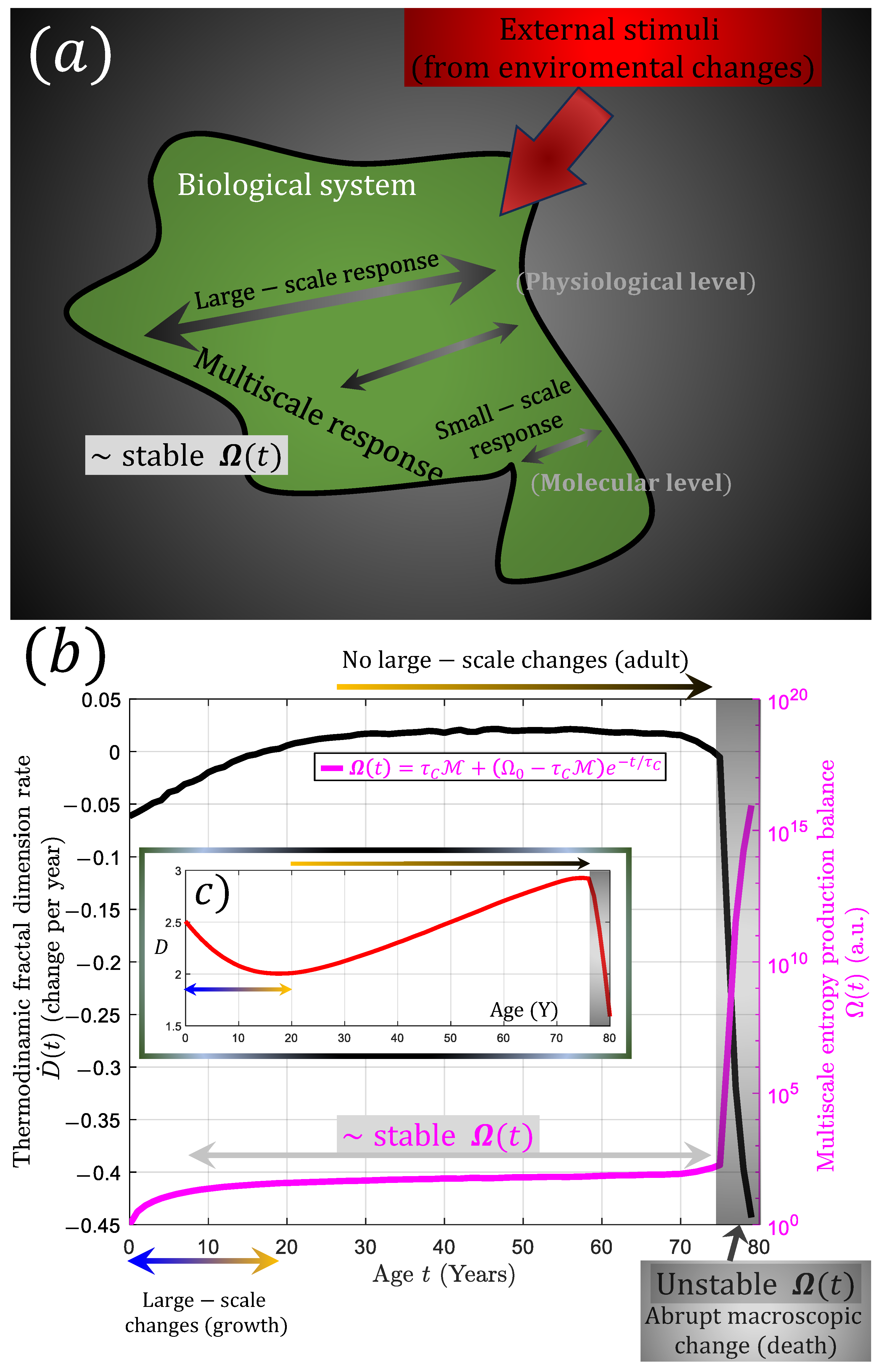
8. Summary and Discussion

The idea that the universe could be made up of multiple systems that interact with each other, and at different scales, may sound like an obvious idea. Especially when we consider that a particular system will react to the influence of other systems. However, the problem with this is that we might interpret the “systems” as macroscopic domains, forgetting that they could also react to other smaller scales. This leads to the transport and release of excess energy to smaller scales. In other words, a microscopic-scale dynamic could exist as a mechanism for energy release without the need to express large changes macroscopically. The lack of clarity regarding the multiscale influence of one system on another leads to the idea that very different disciplines (such as physics, life sciences, and humanities, among others) are in separate fields and their unification is seen as unthinkable or improbable [271,272]. However, new developments in the field of thermodynamics have questioned this separation, so recent efforts seek to unify the sciences under the lens of thermodynamics, stability, and dissipation [273,274,275,276,277,278,279,280,281,282,283]. The way in which excess external energy is dissipated at different scales can be seen as a description that aligns with the perspective of unifying different scientific fields through thermodynamics as parts of a “big history”. Therefore, a global parameter of the multiscale thermodynamics’ lens, such as the thermodynamic fractal dimension, could first exist and, second, have different interpretations in different fields and subfields. This could suggest that multiscale thermodynamics can provide a common foundation for understanding complex systems, regardless of their nature. This is why this work explores the use of multiscale thermodynamic fractal dimensions $D$ in various fields and how this framework can be applied to describe complex systems.

The multiscale thermodynamics concept was described in Equation (2). This explained how external forces generate power laws and geometrical features that can be linked to the balance between small-scale and large-scale entropy production (Section 2). Despite the fact that there have been some works dealing with the fractal dimension and entropy [284,285] or entropy and geometry [286,287], Equation (2) incorporates more general properties than the multiscale description of Onsager’s coefficients and heterogeneous resistivity to understand the relationship between the hierarchies of complex systems, emergent behavior, power laws, and fractal thermodynamics [59]. That is, Equation (2) can be seen as providing a theoretical foundation for the study of multiscale entropy, by linking the dynamic of complex systems across different scales to the concept of entropy production.

The generation of $D$ in terms of multiscale entropy production balance means that the smaller the $D$, the more efficient the system is at dissipating energy at larger scales, which can be observed as macroscopic or emergent behavior in complex systems. In contrast, larger $D$ means that the systems are more efficient at dissipating energy at smaller scales, which, in turn, generates rougher surfaces and networks that fill more the space. For example, in a system of interacting particles, the decrease in $D$ may cause the particles to become more ordered and form patterns, such as crystals [288]. Similarly, in a complex system of organisms, this decreases in $D$ may cause the emergence of ordered patterns of behavior or collective movements, such as flocks of birds or schools of fish. In both cases, it leads to the emergence of macroscopic patterns that cannot be explained by looking at the individual components alone. For example, emergent behaviors are often associated with the formation of a large number of chemical bonds, which are processes that release or dissipate energy. That is, the formation of a crystal is an emergent behavior that occurs when molecules in a liquid come together to form a solid. This process releases energy on a large scale because (almost) all of the molecules in the crystal have a lower free energy than the molecules in the liquid [289]. Similarly, the formation of a cell is another emergent behavior that occurs when molecules in a liquid come together to form an organized structure. For example, DNA has an electric charge, so its dynamics are associated with the search for electrical neutrality [290,291]. This process also releases energy since the molecules in the cell have a lower energy than the molecules in the liquid. This leads to the formation of a living organism being the most complex emergent behavior in the known universe. This is because this process releases a large amount of energy due to the formation of many chemical bonds that release and produce entropy. Thus, the emergent behavior that rises in complex systems can be seen because of the relationship between smaller thermodynamic fractal dimensions and more efficient energy dissipation at larger scales (Section 3). That is why this multiscale perspective could be the key point to understanding a stable complex network [292]. Despite the focus on emergent and macroscopic features, systems could also experience disturbances that affect multiple scales or involve interactions between different scales. For example, Section 4 shows the relationship between $D$ and the fluctuation–dissipation theorem. This theorem describes the (multiscale) spontaneous fluctuations (response) of a system to an external perturbation and, as a consequence, could generate macroscopic patterns. In simple words, the variation of the dissipation could lead to fractal properties [293,294,295]. Here, the multiscale entropy production balance ${\mathsf{\Omega }}_V$ can capture this dynamic by describing the fluctuations and dissipation of energy in both space and time. In particular, the spatial and temporal properties of ${\mathsf{\Omega }}_V$ could reveal how energy is dissipated at different scales and how the system responds to external perturbations, such as Figure 5 shows. In other words, ${\mathsf{\Omega }}_V$ is the factor that relates the interaction of one scale to another within the same system.

Certain systems may not efficiently dissipate the energy that is being injected and instead respond to external inputs by generating multiple losses that amplify the perturbation across multiple scales. That is why Section 5 relates multiscale thermodynamics to chaos theory. This section shows that the $D$ can be linked to the sum of Lyapunov exponents (Equation (6)), which are used to quantify the degree of chaos in a system. This allows one to use $D$ to describe the emergence of chaos in complex systems. In the context of multiscale thermodynamics, it can be observed that the system’s sensitivity to initial conditions is influenced by the dominance of small-scale entropy production, as depicted in Figure 6a,c. However, the effect of initial conditions is limited to specific scales, as illustrated in Figure 6b. This could suggest that chaotic systems are limited to very specific subdomains and that tiny changes could never affect the stability of a system large enough (composed of many scales). In a very broad sense, the fact that the classical world is not directly affected by the variations of the quantum world could be a consequence of the multiscale properties of the universe. In contrast, only systems that are not too sensitive to initial conditions could lead to emergent behavior. One specific manifestation of chaos theory is observed in the phenomenon of turbulence, which can be characterized by self-similar evolution [296]. In this case, Section 6 discusses the relationship between $D$ and the turbulence phenomenon by means of the Equations (7) and (8). The relationship between larger $D$ and larger Reynolds numbers associated with more turbulent regimes is revealed by this analysis because turbulence could emerge in systems that exhibit greater sensitivity to initial conditions as is shown in Figure 6d.

This study further explores other applications of multiscale thermodynamics beyond fundamental physics. As a result, Section 7 provides specific examples of how this theory can be utilized in various systems. One example discussed in Section 7.1 suggests that the expansion of the entire universe can be viewed as an external force that drives the emergence of macroscopic patterns and increased complexity. Equation (2) supports this idea by indicating that as the universe continues to expand, it will generate more complex structures and emergent behavior due to the drop in $D$, in line with Chaisson’s theory of increasing complexity [142]. In terms of geometry, the fractal dimension tends to be interpreted as a measure of how much an object fills the space it contains. For example, an object with a fractal dimension close to 2 will tend to be one that resembles an area, while one close to 1 will approximate a line [297]. Therefore, if the early universe had high values of $D$, it could mean that mass was spread out over space. However, as the universe evolves, $D$ apparently decreases, meaning that the structures that form in the universe will tend to fill less space, or in other words, be more compact to satisfy lower values of $D$. This means that gravity could be interpreted as the mechanism that aggregates mass to prevent it from spreading out over space, while both biological organisms and emergent behaviors could be ways of compacting matter and preventing it from spreading out over the universe. As mass is intimately related to energy [298], this compaction of matter could also imply that energy is stored in a more compact way, which could explain Chaisson’s description that matter stores (compacts) more and more energy as the universe progresses ($D$ decreases). Hence, physical phenomena such as complexity, gravity, or the absence of quantum effects at large scales could be a direct consequence of multiscale thermodynamics. This ongoing emergence, or collaboration, of complex dynamic is also relevant to other theories, such as geology or the evolution of life, which can be seen as a multiscale phenomenon involving biological systems interacting at various levels of organization, from molecular to ecosystem scales and shaped by environmental influences [299,300,301]. In that line, Section 7.2 provides an example of how topography, which refers to the physical characteristics of a landscape, is linked to the fractal dimension of multiscale thermodynamics. This connection is established through the process of energy dissipation and erosion. As an illustration, mountain topography can trap clouds and produce macroscopic rain, leading to smoother surfaces at the mountain base due to erosion (Figure 8). This effect on geological surfaces also impacts other systems such as the process of generating subduction earthquakes. For instance, seafloor irregularities tend to be polished or smoothed when one tectonic plate is subducted beneath another plate [302]. This implies that the deeper zones of faults can become smoother, potentially making them more susceptible to larger earthquakes and precursor activity [302,303,304,305]. In this regard, the non-subducting plate acts as a macroscopic force, which reduces the $D$ of the system by increasing fault smoothness and reducing the resistance to rupture. Furthermore, since $D$ is a global parameter, its decrease not only affects the rupture process [306] but it also increases the generation of microcracks that could lead to fluid migration, emissions of electromagnetic signals, or precursor seismicity [302,307].

Section 7.3 presents another example of Equation (2), which is the transpiration phenomenon in trees. The effective transport of fluids by trees to the atmosphere is an illustration of an external force attempting to establish equilibrium. The self-similar branches of trees signify the effect of external forces, indicating that trees can be viewed as a mechanism to restore the water balance between the soil and the lower atmosphere (Figure 9).

The human body is also a multiscale system, and its macroscopic energy dissipation during growth could also lead to the development of organs characterized by smaller $D$ [308,309]. However, once growth stops in adulthood, macroscopic dissipation ceases, and humans only dissipate energy at the microscopic scale, resulting in an increase in $D$. That is why Section 7.4 and Section 7.5 provide examples of this process. For instance, changes in the DNA structure, which increase with age, reflect small-scale dissipation. The external manifestation of this small-scale dissipation can also be seen in changes in skin surface texture, with smoother skin during growth (macroscopic dissipation dominance) and rougher skin after adulthood (microscopic dissipation dominance). Section 7.5 focuses specifically on the structure of the brain. When growth stops, the increase in $D$ also affects the brain, causing the neural networks to become more complex as one ages, resulting in an improvement in the ability to process information or cognition. However, these small-scale structures can also lead to the generation of fractal noise that may disrupt neural patterns, leading to a decrease in $D$ and a decline in cognitive abilities (as illustrated in Figure 11). In this context, the fractal structure of the brain is considered a result of external stimuli. According to Sloman and Fernbach [310], the thinking process is a means to navigate and respond to the external world, which can increase our chances of survival. This cognitive perspective suggests that the brain and its processes are intimately tied to the environment and that they emerge in response to external factors [311]. Then, the primary function of thinking and the brain increases the external influence as described in Section 7.5. In a similar vein, when a system is uncertain about its environment, a fundamental parameter is its free energy. In the context of the free energy principle, a reduction in free energy could mean that the system is reducing its uncertainty and becoming more efficient at representing and anticipating its surroundings [312,313,314]. Therefore, cognitive capacity increases [315]. In the context of multiscale thermodynamics, a reduction in free energy is aligned with an increase in $D$. Thus, the free energy principle can be seen as a special case of the multiscale dissipation principle. It is important to consider that, as the cooperation process is also linked to brain activity [316], Section 7.6 deals with the evolution of moral rising due to shared goals, which could be regarded as a manifestation of emergent processes that satisfy the increased complexity of the universe. This idea can be applied to this paper itself as it could be viewed as an example of decreasing thermodynamic fractal dimension, as it organizes various topics into a coherent macroscopic theoretical framework.

Section 7.7 leads to the reinterpretation of natural selection in terms of the multiscale thermodynamic principles. For example, organisms evolve through two processes. The first one is the assembly of macroscopic or emergent structures due to the universe’s inherent tendency to decrease the value of $D$. That is, the universe tends to construct larger-scale elements from smaller constituents (emergent behavior) as a means to increase the macroscopic entropy of the universe (Section 7.1 and Section 7.4). The second one come from the fact that this large-scale evolution can be slightly different when considering individual organisms or local environments. For instance, in nature, organisms influence each other [317], which can be seen as external forces from the environment (not external from the universe). This is similar to what is demonstrated regarding the effect of external stimuli at the cellular level in Section 7.5. This implies that an organism’s adaptation directly stems from molecular or cellular changes in response to an environmental force. In other words, an external force (the environment) prompts the organism to release excess energy at both microscopic (molecular or cellular changes) and macroscopic (physiological or behavioral) levels. Therefore, the concept known as adaptation is, in this perspective, the multiscale response to an external force. Put differently, adaptation is the energy dissipation mechanism across different scales that an organism employs to continue reducing the thermodynamic fractal dimension of the universe under local conditions.

This perspective leads to the equation for multiscale homeostatic imbalance shown in Equation (10). This equation describes how energy dissipation can occur differently at different scales within an organism, leading to flow and dynamics within the organism. Figure 12b,c show that an organism can survive because the “imbalance” $\mathsf{\Omega }$ remains relatively constant throughout life. This is, in part, justified by the fact that chaotic systems (if we consider an organism to be chaotic) are sensitive to initial conditions but their effects do not extend to all scales, which allows for macroscopic stability or “robustness” (Section 5 and Section 7.7). However, as an organism dies, its effect can manifest as a drastic change in $D$. For example, $D$ will tend to decrease dramatically if a generalized system-wide death mechanism, such as apoptosis or necrosis, is taking place. That is, $D$ will influence $\mathsf{\Omega }$ in such a way that $\mathsf{\Omega }$ will cease to be constant and diverge (black area in Figure 12b). Then, the concept of considering that a system can respond to different scales given an external force also seems to be applicable to biological systems, since it allows us to describe fundamental processes in the same way that it can describe physical or social systems. For this reason, the multiscale formalism seems to be a prevalent principle in nature. Note that the explanation (or reinterpretation) of complex processes such as life, death, aging, topography, chaos, cosmic evolution, or turbulence are based on systems with many components and scales. Therefore, we have not considered the effects of only one particular scale. This means that we have not described the evolution of individual particles, which would lead to the description of fundamental forces or quantum level. Therefore, the multiscale principle cannot be considered a “theory of everything,” but rather a principle that is applicable to systems with many constituents with irreversible or dissipative properties. That is, the theory is only applicable to multiscale systems and could be considered a direct application of Newton’s second and third laws.

Lastly, it is important to remember that what we present in this work aligns more with a principle than a method. This is because a principle refers to a fundamental rule that serves as a broad foundation within a field, integrating existing knowledge. On the other hand, methods aim to solve specific problems through a series of actions. Additionally, this multiscale principle could be called luxuriæ, which is a Latin word that means “out of place.” We interpret this as a way of saying that a system expels or dissipates energy. A specific application of the luxuriæ principle in a methodology can be found in solid mechanics. For instance, the generation, localization, and coalescence of cracks before macroscopic failure in a rock sample has been a phenomenon lacking a complete explanation due to the complexity of the involved mechanisms. Nevertheless, multiscale thermodynamics have offered a tool that elucidates this process [53,59]. For instance, this perspective is based on the heterogeneous resistivity of the rock material, which generates differential stresses and microcracks to dissipate energy at a smaller scale. As stresses increase without causing macroscopic deformation, these microcracks interact, creating pathways for fluids and chemical changes, allowing the formation of larger cracks and, ultimately, macroscopic failure. Subsequently, the parameter of the thermodynamic fractal dimension ($D$) is employed to describe the relationship between large-scale energy release and macroscopic failure by establishing analytical relationships between the fault area $A$ and $D$ ($A=A\left(D\right)$). In the case of a rupture in a pre-existing macroscopic fault, analytical relationships with changes in fault geometry can also be found. This implies that the luxuriæ principle applied to solid failure is capable of fully explaining the failure process as it posits that a decrease in $D$ leads to crack localization, while the contact area in pre-existing faults becomes smoother, resulting in reduced rupture resistance. Thus, it quantitatively links effects and parameters that other descriptions are unable to achieve. This example could inspire other areas that have not been covered in this work to use the luxuriæ principle as a tool for future development and research.

9. Conclusions

Multiscale thermodynamics is a framework that could be used to study systems with a wide range of scales. Its application to various systems, including trees, turbulence, emergent behavior, chaos theory, human organs, aging, DNA structural evolution, topographical structures, the universe expansion, and the generation of complexity, could generate significant consequences.

First, the universe is full of systems that are composed of many scales. This implies that interactions between these systems could generate responses at scales that are not necessarily evidently macroscopically. This could be a common characteristic of many systems, which could allow us to describe them based on this fact.

Second, many complex (open) systems are characterized by the coordinated dynamic of many of their constituents, which indicates that they have energetic constraints that lead to similar evolution known as emergent behavior. This can be described as the dissipation of energy at the macroscopic scale, which leads to low values of $D$. In other words, emergent behaviors could occur when systems are more efficient at releasing excess energy in a macroscopic way. Additionally, multiscale systems can also have medium or high values of $D$, which would imply that the dissipation of energy at small scales could also be relevant in these systems. In this way, systems that are described by power laws could be the consequence of a balance of energy dissipation at different scales against an external force that generates an excess of energy.

Third, chaotic systems could be restricted to certain subdomains. This is because small perturbations in the initial conditions could be smoothed out at larger scales, indicating that when a system is composed of a wide range of scales, changes at small scales would not affect the macroscopic structure of the system. This could explain why many biological systems do not undergo rapid macroscopic changes despite the existence of a vigorous molecular or cellular dynamic. In other words, multiscale thermodynamics allows us to define the macroscopic stability of systems. In the extreme case, it could explain why the classical world is not affected by fluctuations or changes at the quantum level.

Fourth, the universe appears to be decreasing its $D$, which would indicate that it is more efficient at releasing energy at increasingly larger scales. This implies three things. First, the universe could be affected by an unknown external force. More studies are needed to understand the meaning of the word “external” in this context. Second, all subsystems should tend to have a lower $D$. This means that systems should have more emergent behaviors as the universe progresses. This can also be seen in surfaces that tend to be smoother. Thus, it could physically explain the role of erosion in nature. Finally, a universe with a lower $D$ also implies, in geometric terms, that matter must occupy less space in the universe. This could directly link the force of gravity to macroscopic dissipation. That is, gravity could be regarded a dissipative force. Since this compaction of mass could also generate the compaction of energy, the fact that mass is storing more and more energy could mean that the complexity of the universe is a direct manifestation of an expanding universe that produces low $D$ values.

Fifth, the multiscale description of the universe allows us to redefine theories associated with life, such as evolution or natural selection. As the universe could foster emergent structures in irreversible conditions, it could be that life itself is a consequence of an expanding universe. Locally, organisms are affected by environmental conditions, which can be reinterpreted as external forces that affect the most microscopic scales of the organism (genes and cells), which could generate macroscopic changes only over long periods of time to overcome the scale restriction described for chaotic systems (point three). As the universe also encourages the dissipation of energy, only those organisms that are better at dissipating macroscopic energy will be able to survive (the proper macroscopic changes). In this way, microscopic changes due to external forces (stimuli) promote physical or behavioral changes only when they are more efficient at dissipating macroscopic energy. Thus, natural selection and evolution could be a consequence, or one form, of multiscale dissipation.

Sixth, organisms also undergo macroscopic changes during growth, which defines the structure of their organs. In this way, during growth, $D$ is small, which implies that the organs (skin, brain, lungs, etc.) act in an emergent and collaborative manner. This manifests itself in smoother skin and brains with lower cognitive abilities. When an organism reaches maturity, $D$ increases, which generates an increase in cognitive abilities, health problems, and eventually the death of the organism. Therefore, the theory of multiscale thermodynamics could clarify why biological systems tend to emerge, grow, and eventually perish. In this way, life can be seen as a dissipative process that can be studied from the equation of homeostasis (Equation (10)). In less scientific words, life could just be a form of “disorder”.

Finally, in view of the wide range of applications in which multiscale thermodynamics is found, as was shown in this work by transcribing and reinterpreting several and different systems under the lens of multiscale thermodynamics, it can be concluded that there are indications of a new principle in nature that can be described in a general manner as:

“Systems that interact with each other can trigger responses at multiple scales as a manner to dissipate the excess energy that comes from this interaction”.

This principium luxuriæ (from the Latin word ‘Luxus’, which means ‘out of place’ in the sense that the energy tends to be spread out, and ‘principium’, which means principle), through an open system, allows us to explain the internal dynamics of complex systems that generate high complexity, as well as the emergent behaviors, self-organization, and adaptation of systems. The future challenges of multiscale thermodynamics include developing a more complete understanding of how the fractal dimension of complex systems changes over time, as well as exploring new applications of this theory to other scientific fields. A special point is associated to keep studying the mathematical properties of the thermodynamic fractal dimension as well the quantification of the entropy production balance described by Equation (2). Additionally, the development of new mathematical tools and techniques will be necessary to make predictions about their future outputs. Ultimately, the multiscale thermodynamics fractal dimension theory holds great promise for advancing our understanding of multiscale complex systems, fractals, and life processes and for unlocking new insights into the behavior of the universe as a whole.

References

1. Bar-Yam, Y. Dynamics of Complex Systems; Westview Press: Boulder, CO, USA, 2003. [Google Scholar]
2. Boccara, N. Modeling Complex Systems; Springer: New York, NY, USA, 2010. [Google Scholar]
3. West, G.B. Scale: The Universal Laws of Growth, Innovation, Sustainability, and the Pace of Life in Organisms, Cities, Economies, and Companies; Penguin Press: London, UK, 2017. [Google Scholar]
4. Ladyman, J.; Wiesner, K. What is a Complex System? Yale University Press: New Haven, CT, USA, 2020. [Google Scholar] [CrossRef]
5. Vitiello, G. Fractals, coherent states and self-similarity induced noncommutative geometry. Phys. Lett. A 2012, 376, 2527–2532. [Google Scholar] [CrossRef]
6. Nigmatullin, R.R.; Chen, Y. Self-Similarity Principle and the General Theory of Fractal Elements: How to Fit a Random Curve with a Clearly Expressed Trend? Mathematics 2023, 11, 2781. [Google Scholar] [CrossRef]
7. Pinto, C.M.; Lopes, A.M.; Machado, J.T. Double power laws, fractals and self-similarity. Appl. Math. Model. 2014, 38, 4019–4026. [Google Scholar] [CrossRef]
8. Ziepke, A.; Maryshev, I.; Aranson, I.S.; Frey, E. Multi-scale organization in communicating active matter. Nat. Commun. 2022, 13, 6727. [Google Scholar] [CrossRef] [PubMed]
9. Yao, Z.; Lundqvist, E.; Kuang, Y.; Ardoña, H.A.M. Engineering Multi-Scale Organization for Biotic and Organic Abiotic Electroactive Systems. Adv. Sci. 2023, 10, 2205381. [Google Scholar] [CrossRef] [PubMed]
10. An, G. Introduction of an agent-based multi-scale modular architecture for dynamic knowledge representation of acute inflammation. Theor. Biol. Med. Model. 2008, 5, 11. [Google Scholar] [CrossRef] [PubMed]
11. Buizer, M.; Arts, B.; Kok, K. Governance, Scale and the Environment: The Importance of Recognizing Knowledge Claims in Transdisciplinary Arenas. Ecol. Soc. 2011, 16, 21. [Google Scholar] [CrossRef]
12. del Castillo, L.F.; Vera-Cruz, P. Thermodynamic Formulation of Living Systems and Their Evolution. J. Mod. Phys. 2011, 02, 379–391. [Google Scholar] [CrossRef]
13. Gatti, R.C. The fractal nature of the latitudinal biodiversity gradient. Biologia 2016, 71, 669–672. [Google Scholar] [CrossRef]
14. Yu, J.S.; Bagheri, N. Multi-class and multi-scale models of complex biological phenomena. Curr. Opin. Biotechnol. 2016, 39, 167–173. [Google Scholar] [CrossRef]
15. Schaffer, L.V.; Ideker, T. Mapping the multiscale structure of biological systems. Cell Syst. 2021, 12, 622–635. [Google Scholar] [CrossRef] [PubMed]
16. Einstein, A. Bemerkung zu der Franz Seletyschen Arbeit “Beiträge zum kosmologischen System”. Ann. Phys. 1922, 374, 436–438. [Google Scholar] [CrossRef]
17. Bremer, K.; Wanntorp, H.-E. Hierarchy and Reticulation in Systematics. Syst. Zool. 1979, 28, 624. [Google Scholar] [CrossRef]
18. Cilliers, P. Boundaries, Hierarchies and Networks in Complex Systems. Int. J. Innov. Manag. 2001, 5, 135–147. [Google Scholar] [CrossRef]
19. Chen, Y.; Zhou, Y. The Rank-Size Rule and Fractal Hierarchies of Cities: Mathematical Models and Empirical Analyses. Environ. Plan. B Plan. Des. 2003, 30, 799–818. [Google Scholar] [CrossRef]
20. Pavé, A. Biological and Ecological Systems Hierarchical Organisation. In Hierarchy in Natural and Social Sciences Methodos Series; Pumain, D., Ed.; Springer: Dordrecht, The Netherlands, 2006. [Google Scholar] [CrossRef]
21. Beck, F.; Burch, M.; Munz, T.; Di Silvestro, L.; Weiskopf, D. Generalized Pythagoras Trees: A Fractal Approach to Hierarchy Visualization. In Computer Vision, Imaging and Computer Graphics—Theory and Applications; VISIGRAPP Communications in Computer and Information Science; Battiato, S., Coquillart, S., Pettré, J., Laramee, R., Kerren, A., Braz, J., Eds.; Springer: Cham, Switzerland, 2015. [Google Scholar] [CrossRef]
22. Komvopoulos, K. A Multiscale Theoretical Analysis of the Mechanical, Thermal, and Electrical Characteristics of Rough Contact Interfaces Demonstrating Fractal Behavior. Front. Mech. Eng. 2020, 6, 36. [Google Scholar] [CrossRef]
23. Dos Anjos, P.H.R.; Gomes-Filho, M.S.; Alves, W.S.; Azevedo, D.L.; Oliveira, F.A. The Fractal Geometry of Growth: Fluctuation–Dissipation Theorem and Hidden Symmetry. Front. Phys. 2021, 9, 741590. [Google Scholar] [CrossRef]
24. Dublanchet, P. Shear Stress and b-value Fluctuations in a Hierarchical Rate-and-State Asperity Model. Pure Appl. Geophys. 2022, 179, 2423–2435. [Google Scholar] [CrossRef]
25. Kovchegov, Y.; Zaliapin, I.; Foufoula-Georgiou, E. Random Self-Similar Trees: Emergence of Scaling Laws. Surv. Geophys. 2022, 43, 353–421. [Google Scholar] [CrossRef]
26. Mohanty, V.; Greenbury, S.F.; Sarkany, T.; Narayanan, S.; Dingle, K.; Ahnert, S.E.; Louis, A.A. Maximum mutational robustness in genotype–phenotype maps follows a self-similar blancmange-like curve. J. R. Soc. Interface 2023, 20, 20230169. [Google Scholar] [CrossRef]
27. Brown, J.H.; Gupta, V.K.; Li, B.-L.; Milne, B.T.; Restrepo, C.; West, G.B. The fractal nature of nature: Power laws, ecological complexity and biodiversity. Philos. Trans. R. Soc. B Biol. Sci. 2002, 357, 619–626. [Google Scholar] [CrossRef] [PubMed]
28. West, G.B. Size, Scale and the Boat Race; Conceptions, Connections and Misconceptions. In Hierarchy in Natural and Social Sciences; Methodos Series; Pumain, D., Ed.; Springer: Dordrecht, The Netherlands, 2006. [Google Scholar] [CrossRef]
29. Sales-Pardo, M.; Guimerà, R.; Moreira, A.A.; Amaral, L.A.N. Extracting the hierarchical organization of complex systems. Proc. Natl. Acad. Sci. USA 2007, 104, 15224–15229. [Google Scholar] [CrossRef] [PubMed]
30. Corominas-Murtra, B.; Goñi, J.; Solé, R.V.; Rodríguez-Caso, C. On the origins of hierarchy in complex networks. Proc. Natl. Acad. Sci. USA 2013, 110, 13316–13321. [Google Scholar] [CrossRef] [PubMed]
31. Johnson, C.W. What are emergent properties and how do they affect the engineering of complex systems? Reliab. Eng. Syst. Saf. 2006, 91, 1475–1481. [Google Scholar] [CrossRef]
32. Luo, J.; Magee, C.L. Detecting evolving patterns of self-organizing networks by flow hierarchy measurement. Complexity 2011, 16, 53–61. [Google Scholar] [CrossRef]
33. San Martin, D. Clarity: Un Modelo Unificador de las Ciencias…y un Relato del Todo; Planeta Editor: Barcelona, Spain, 2021. (In Spanish) [Google Scholar]
34. Marković, D.; Gros, C. Power laws and self-organized criticality in theory and nature. Phys. Rep. 2014, 536, 41–74. [Google Scholar] [CrossRef]
35. Bejan, A.; Lorente, S. Constructal law of design and evolution: Physics, biology, technology, and society. J. Appl. Phys. 2013, 113, 151301. [Google Scholar] [CrossRef]
36. Lopes, A.M.; Machado, J.A.T. Power Law Behaviour in Complex Systems. Entropy 2018, 20, 671. [Google Scholar] [CrossRef]
37. Ortman, S.G.; Lobo, J.; Smith, M.E. Cities: Complexity, theory and history. PLoS ONE 2020, 15, e0243621. [Google Scholar] [CrossRef]
38. Bashkirov, A.; Vityazev, A. Information entropy and power-law distributions for chaotic systems. Phys. A Stat. Mech. Its Appl. 1998, 277, 136–145. [Google Scholar] [CrossRef]
39. Chen, Y. The rank-size scaling law and entropy-maximizing principle. Phys. A Stat. Mech. Its Appl. 2012, 391, 767–778. [Google Scholar] [CrossRef]
40. Curado, E.M.F.; Nobre, F.D.; Plastino, A. Associating an Entropy with Power-Law Frequency of Events. Entropy 2018, 20, 940. [Google Scholar] [CrossRef] [PubMed]
41. Jin, C.; Song, C.; Bjelland, J.; Canright, G.; Wang, D. Emergence of scaling in complex substitutive systems. Nat. Hum. Behav. 2019, 3, 837–846. [Google Scholar] [CrossRef]
42. Nosonovsky, M.; Roy, P. Scaling in Colloidal and Biological Networks. Entropy 2020, 22, 622. [Google Scholar] [CrossRef] [PubMed]
43. Jahanmiri, F.; Parker, D.C. An Overview of Fractal Geometry Applied to Urban Planning. Land 2022, 11, 475. [Google Scholar] [CrossRef]
44. Wawrzaszek, A.; Modzelewska, R.; Krasińska, A.; Gil, A.; Glavan, V. Fractal Dimension Analysis of Earth Magnetic Field during 26 August 2018 Geomagnetic Storm. Entropy 2022, 24, 699. [Google Scholar] [CrossRef]
45. Newman, M.E.J. Power laws, Pareto distributions and Zipf’s law. Contemp. Phys. 2005, 46, 323–351. [Google Scholar] [CrossRef]
46. Abe, S.; Suzuki, N. Scale-free network of earthquakes. EPL 2004, 65, 581–586. [Google Scholar] [CrossRef]
47. Song, C.; Havlin, S.; Makse, H.A. Self-similarity of complex networks. Nature 2005, 433, 392–395. [Google Scholar] [CrossRef]
48. Wang, B.; Zhu, J.; Wei, D. The self-similarity of complex networks: From the view of degree–degree distance. Mod. Phys. Lett. B 2021, 35, 2150331. [Google Scholar] [CrossRef]
49. Pastor-Satorras, R.; Wagensberg, J. The maximum entropy principle and the nature of fractals. Phys. A Stat. Mech. Its Appl. 1998, 251, 291–302. [Google Scholar] [CrossRef]
50. Tate, N.J. Maximum entropy spectral analysis for the estimation of fractals in topography. Earth Surf. Process. Landf. 1999, 23, 1197–1217. [Google Scholar] [CrossRef]
51. Dover, Y. A short account of a connection of power laws to the information entropy. Phys. A Stat. Mech. Its Appl. 2004, 334, 591–599. [Google Scholar] [CrossRef]
52. Grmela, M. Multiscale Thermodynamics. Entropy 2021, 23, 165. [Google Scholar] [CrossRef] [PubMed]
53. Venegas-Aravena, P.; Cordaro, E.G.; Laroze, D. Natural Fractals as Irreversible Disorder: Entropy Approach from Cracks in the Semi Brittle-Ductile Lithosphere and Generalization. Entropy 2022, 24, 1337. [Google Scholar] [CrossRef]
54. Gokcen, N.A.; Reddy, R.G. Entropy and Related Functions. In Thermodynamics; Springer: Boston, MA, USA, 1996. [Google Scholar] [CrossRef]
55. Lebowitz, J.L. Emergent phenomena. Phys. J. 2007, 6, 41. [Google Scholar]
56. Atmanspacher, H. On Macrostates in Complex Multi-Scale Systems. Entropy 2016, 18, 426. [Google Scholar] [CrossRef]
57. Adams, A.M. A graph-theoretic approach to understanding emergent behavior in physical systems. In Proceedings of the ALIFE 2021: The 2021 Conference on Artificial Life, Online, 18–22 July 2021; ASME: New York, NY, USA, 2021; p. 63. [Google Scholar] [CrossRef]
58. Redondo, J.M.; Garcia, J.S.; Bustamante-Zamudio, C.; Pereira, M.F.; Trujillo, H.F. Heterogeneity: Method and applications for complex systems analysis. J. Physics Conf. Ser. 2022, 2159, 012013. [Google Scholar] [CrossRef]
59. Venegas-Aravena, P.; Cordaro, E.; Laroze, D. Fractal Clustering as Spatial Variability of Magnetic Anomalies Measurements for Impending Earthquakes and the Thermodynamic Fractal Dimension. Fractal Fract. 2022, 6, 624. [Google Scholar] [CrossRef]
60. Mandelbrot, B.B. The Fractal Geometry of Nature; W. H. Freeman and Company: New York, NY, USA, 1982. [Google Scholar]
61. Newton, I. Philosophiae Naturalis Principia Mathematica; Smithsonian Institution: Washington, DC, USA, 1687. [Google Scholar]
62. Onsager, L. Reciprocal Relations in Irreversible Processes. I. Phys. Rev. 1931, 37, 405–426. [Google Scholar] [CrossRef]
63. Onsager, L. Reciprocal Relations in Irreversible Processes. II. Phys. Rev. B 1931, 38, 2265–2279. [Google Scholar] [CrossRef]
64. Boltzmann, L. “Über die Mechanische Bedeutung des Zweiten Hauptsatzes der Wärmetheorie” (german). Wien. Berichte 1866, 53, 195–220. [Google Scholar]
65. Callen, H.B. Thermodynamics and an Introduction to Thermostatistics; Wiley: New York, NY, USA, 1960. [Google Scholar]
66. De Groot, S.R.; Mazur, P. Nonequilibrium Thermodynamics; North-Holland Pub. Co.: Amsterdam, The Netherlands, 1962. [Google Scholar]
67. Frisch, D.H. The Microscopic Interpretation of Entropy. Am. J. Phys. 1966, 34, 1171–1173. [Google Scholar] [CrossRef]
68. Riek, R. A Derivation of a Microscopic Entropy and Time Irreversibility from the Discreteness of Time. Entropy 2014, 16, 3149–3172. [Google Scholar] [CrossRef]
69. Sahimi, M.; Arbabi, S. Scaling Laws for Fracture of Heterogeneous Materials and Rock. Phys. Rev. Lett. 1996, 77, 3689–3692. [Google Scholar] [CrossRef]
70. Vallianatos, F.; Tzanis, A. On the nature, scaling and spectral properties of pre-seismic ULF signals. Nat. Hazards Earth Syst. Sci. 2003, 3, 237–242. [Google Scholar] [CrossRef]
71. Anastasiadis, C.; Triantis, D.; Stavrakas, I.; Vallianatos, F. Pressure Stimulated Currents (PSC) in marble samples. Ann. Geophys. 2009, 47, 21–28. [Google Scholar] [CrossRef]
72. Kuksenko, V.; Tomilin, N.; Chmel, A. The role of driving rate in scaling characteristics of rock fracture. J. Stat. Mech. Theory Exp. 2005, 2005, P06012. [Google Scholar] [CrossRef]
73. Malakhovsky, I.; Michels, M.A.J. Scaling and localization in fracture of disordered central-force spring lattices: Comparison with random damage percolation. Phys. Rev. B 2006, 74, 014206. [Google Scholar] [CrossRef]
74. Triantis, D.; Vallianatos, F.; Stavrakas, I.; Hloupis, G. Relaxation phenomena of electrical signal emissions from rock following application of abrupt mechanical stress. Ann. Geophys. 2012, 55, 207–212. [Google Scholar] [CrossRef]
75. Venegas-Aravena, P.; Cordaro, E.G.; Laroze, D. A review and upgrade of the lithospheric dynamics in context of the seismo-electromagnetic theory. Nat. Hazards Earth Syst. Sci. 2019, 19, 1639–1651. [Google Scholar] [CrossRef]
76. Potirakis, S.M.; Contoyiannis, Y.; Eftaxias, K.; Melis, N.S.; Nomicos, C. Post-spontaneous-symmetry-breaking power-laws after a very strong earthquake: Indication for the preparation of a new strong earthquake or not? Phys. A Stat. Mech. Its Appl. 2021, 589, 126607. [Google Scholar] [CrossRef]
77. Loukidis, A.; Tzagkarakis, D.; Kyriazopoulos, A.; Stavrakas, I.; Triantis, D. Correlation of Acoustic Emissions with Electrical Signals in the Vicinity of Fracture in Cement Mortars Subjected to Uniaxial Compressive Loading. Appl. Sci. 2022, 13, 365. [Google Scholar] [CrossRef]
78. Yang, C.; Wu, Z.; Wang, W.; Qu, H.; Ren, N.; Li, H. Study on the influence of natural cracks on the mechanical properties and fracture mode for shale at the microscale: An example from the Lower Cambrian Niutitang Formation in northern Guizhou. Front. Earth Sci. 2023, 10, 1032817. [Google Scholar] [CrossRef]
79. Mandelbrot, B.B. Negative fractal dimensions and multifractals. Phys. A Stat. Mech. Its Appl. 1990, 163, 306–315. [Google Scholar] [CrossRef]
80. Dvoretskaya, O.A.; Kondratenko, P.S. Anomalous transport in fractal media with randomly inhomogeneous diffusion barrier. Cond-Mat. Soft 2013, 103, 325–339. [Google Scholar] [CrossRef]
81. Chen, Y.; Yang, H. Numerical simulation and pattern characterization of nonlinear spatiotemporal dynamics on fractal surfaces for the whole-heart modeling applications. Eur. Phys. J. B 2016, 89, 181. [Google Scholar] [CrossRef]
82. Yang, H. The Generator of Fractal Surfaces or Images, MATLAB Central File Exchange. Available online: https://www.mathworks.com/matlabcentral/fileexchange/78179-the-generator-of-fractal-surfaces-or-images (accessed on 30 August 2023).
83. Greiner, W.; Neise, L.; Stöcker, H. Number of Microstates Ω and Entropy S. In Thermodynamics and Statistical Mechanics. Classical Theoretical Physics; Springer: New York, NY, USA, 1995. [Google Scholar] [CrossRef]
84. Nicolis, G.; Prigogine, I. Self-Organization in Nonequilibrium Systems: From Dissipative Structures to Order through Fluctuations, 1st ed.; Wiley: Hoboken, NJ, USA, 1977. [Google Scholar]
85. Heylighen, F. The science of self-organization and adaptivity. Encycl. Life Support Syst. 2001, 5, 253–280. [Google Scholar]
86. De Wolf, T.; Holvoet, T. Emergence Versus Self-Organisation: Different Concepts but Promising When Combined. In Engineering Self-Organising Systems. ESOA Lecture Notes in Computer Science; Brueckner, S.A., Di Marzo Serugendo, G., Karageorgos, A., Nagpal, R., Eds.; Springer: Berlin/Heidelberg, Germany, 2005. [Google Scholar] [CrossRef]
87. Addiscott, T. Entropy, non-linearity and hierarchy in ecosystems. Geoderma 2010, 160, 57–63. [Google Scholar] [CrossRef]
88. Cavagna, A.; Cimarelli, A.; Giardina, I.; Parisi, G.; Santagati, R.; Stefanini, F.; Viale, M. Scale-free correlations in starling flocks. Proc. Natl. Acad. Sci. USA 2010, 107, 11865–11870. [Google Scholar] [CrossRef]
89. Gershenson, C.; Polani, D.; Martius, G. Editorial: Complexity and Self-Organization. Front. Robot. AI 2021, 8, 2021. [Google Scholar] [CrossRef]
90. Navarrete, Y.; Davis, S. Quantum Mutual Information, Fragile Systems and Emergence. Entropy 2022, 24, 1676. [Google Scholar] [CrossRef] [PubMed]
91. Cottam, R.; Vounckx, R. Entropy is better related to unification than to order. Biosystems 2023, 223, 104815. [Google Scholar] [CrossRef] [PubMed]
92. Newman, D.V. Emergence and Strange Attractors. Philos. Sci. 1996, 63, 245–261. [Google Scholar] [CrossRef]
93. Bedau, M.A. Weak emergence. In Philosophical Perspectives: Mind, Causation, and World; Tomberlin, J., Ed.; Blackwell: Malden, MA, USA, 1997; Volume 31, pp. 375–399. [Google Scholar] [CrossRef]
94. Nolte, D.D. The tangled tale of phase space. Phys. Today 2010, 63, 33–38. [Google Scholar] [CrossRef]
95. Oprisan, S.A.; Lynn, P.E.; Tompa, T.; Lavin, A. Low-dimensional attractor for neural activity from local field potentials in optogenetic mice. Front. Comput. Neurosci. 2015, 9, 125. [Google Scholar] [CrossRef] [PubMed]
96. Nabika, H.; Itatani, M.; Lagzi, I. Pattern Formation in Precipitation Reactions: The Liesegang Phenomenon. Langmuir 2019, 36, 481–497. [Google Scholar] [CrossRef]
97. Medina, M.; Huffaker, R.; Muñoz-Carpena, R.; Kiker, G. An empirical nonlinear dynamics approach to analyzing emergent behavior of agent-based models. AIP Adv. 2021, 11, 035133. [Google Scholar] [CrossRef]
98. Jirsa, V.; Sheheitli, H. Entropy, free energy, symmetry and dynamics in the brain. J. Phys. Complex. 2022, 3, 015007. [Google Scholar] [CrossRef]
99. Callen, H.B.; Welton, T.A. Irreversibility and Generalized Noise. Phys. Rev. B 1951, 83, 34–40. [Google Scholar] [CrossRef]
100. Kubo, R. The fluctuation-dissipation theorem. Rep. Prog. Phys. 1966, 29, 255–284. [Google Scholar] [CrossRef]
101. Prost, J.; Joanny, J.-F.; Parrondo, J.M.R. Generalized Fluctuation-Dissipation Theorem for Steady-State Systems. Phys. Rev. Lett. 2009, 103, 090601. [Google Scholar] [CrossRef] [PubMed]
102. Turing, A.M. The chemical basis of morphogenesis. Philos. Trans. Roy Soc. Lond Ser. B 1952, 237, 37–72. [Google Scholar] [CrossRef]
103. Miller, D.G. Thermodynamics of Irreversible Processes. The Experimental Verification of the Onsager Reciprocal Relations. Chem. Rev. 1960, 60, 15–37. [Google Scholar] [CrossRef]
104. De Corato, M.; Pagonabarraga, I. Onsager reciprocal relations and chemo-mechanical coupling for chemically active colloids. J. Chem. Phys. 2022, 157, 084901. [Google Scholar] [CrossRef] [PubMed]
105. O’Shaughnessy, B.; Procaccia, I. Analytical Solutions for Diffusion on Fractal Objects. Phys. Rev. Lett. 1985, 54, 455–458. [Google Scholar] [CrossRef] [PubMed]
106. Qian, L.H.; Chen, M.W. Ultrafine nanoporous gold by low-temperature dealloying and kinetics of nanopore formation. Appl. Phys. Lett. 2007, 91, 083105. [Google Scholar] [CrossRef]
107. Erlebacher, J. Mechanism of Coarsening and Bubble Formation in High-Genus Nanoporous Metals. Phys. Rev. Lett. 2011, 106, 225504. [Google Scholar] [CrossRef]
108. Wada, T.; Kato, H. Three-dimensional open-cell macroporous iron, chromium and ferritic stainless steel. Scr. Mater. 2013, 68, 723–726. [Google Scholar] [CrossRef]
109. Geslin, P.-A.; McCue, I.; Gaskey, B.; Erlebacher, J.; Karma, A. Topology-generating interfacial pattern formation during liquid metal dealloying. Nat. Commun. 2015, 6, 8887. [Google Scholar] [CrossRef]
110. Olsen, K.S.; Campbell, J.M. Diffusion Entropy and the Path Dimension of Frictional Finger Patterns. Front. Phys. 2020, 8, 83. [Google Scholar] [CrossRef]
111. Heller, P. Experimental investigations of critical phenomena. Rep. Prog. Phys. 1967, 30, 731. [Google Scholar] [CrossRef]
112. Hohenberg, P.C.; Halperin, B.I. Theory of dynamic critical phenomena. Rev. Mod. Phys. 1977, 49, 435–479. [Google Scholar] [CrossRef]
113. Dorogovtsev, S.N.; Goltsev, A.V.; Mendes, J.F.F. Critical phenomena in complex networks. Rev. Mod. Phys. 2008, 80, 1275–1335. [Google Scholar] [CrossRef]
114. Dorogovtsev, S.N.; Mendes, J.F.F. The Nature of Complex Networks; Oxford University Press (OUP): Oxford, UK, 2022; ISBN 0199695113. [Google Scholar]
115. Potirakis, S.M.; Papadopoulos, P.; Matiadou, N.-L.; Hanias, M.P.; Stavrinides, S.G.; Balasis, G.; Contoyiannis, Y. Spontaneous Symmetry Breaking in Systems Obeying the Dynamics of On–Off Intermittency and Presenting Bimodal Amplitude Distributions. Symmetry 2023, 15, 1448. [Google Scholar] [CrossRef]
116. Nishimori, H.; Ortiz, G. Elements of Phase Transitions and Critical Phenomena; Oxford University Press (OUP): Oxford, UK, 2010; ISBN 9780199577224. [Google Scholar]
117. Halperin, B.I. Theory of dynamic critical phenomena. Phys. Today 2019, 72, 42–43. [Google Scholar] [CrossRef]
118. Fisher, M.E. Critical Phenomena: Proceedings, Stellenbosch, South Africa, 1982; Hahne, F.J.W., Ed.; Springer: Berlin/Heidelberg, Germany, 1983. [Google Scholar]
119. Chen, H.; Yue, Z.; Ren, D.; Zeng, H.; Wei, T.; Zhao, K.; Yang, R.; Qiu, P.; Chen, L.; Shi, X. Thermal Conductivity during Phase Transitions. Adv. Mater. 2018, 31, e1806518. [Google Scholar] [CrossRef]
120. Pietruszka, M.; Olszewska, M. Extracellular ionic fluxes suggest the basis for cellular life at the 1/f ridge of extended criticality. Eur. Biophys. J. 2020, 49, 239–252. [Google Scholar] [CrossRef]
121. Pietruszka, M.A. Non-equilibrium phase transition at a critical point of human blood. Sci. Rep. 2021, 11, 1–8. [Google Scholar] [CrossRef]
122. Schroeder, M. Fractals, Chaos, Power Laws: Minutes from an Infinite Paradise; W.H. Freeman and Company: New York, NY, USA, 1991. [Google Scholar]
123. Moore, B.J. Chaos Theory: Unpredictable Order in Chaos. In Shaking the Invisible Hand; Palgrave Macmillan: London, UK, 2006. [Google Scholar] [CrossRef]
124. Eppel-Meichlinger, J.; Kobleder, A.; Mayer, H. Developing a theoretical definition of self-organization: A principle-based concept analysis in the context of uncertainty in chronic illness. Nurs. Forum 2022, 57, 954–962. [Google Scholar] [CrossRef]
125. Ottino, J.M.; Muzzio, F.J.; Tjahjadi, M.; Franjione, J.G.; Jana, S.C.; Kusch, H.A. Chaos, Symmetry, and Self-Similarity: Exploiting Order and Disorder in Mixing Processes. Science 1992, 257, 754–760. [Google Scholar] [CrossRef]
126. Lorenz, E. The Essence of Chaos; University of Washington Press: Seattle, DA, USA, 1993; pp. 181–206. [Google Scholar]
127. Ruelle, D. Chaotic Evolution and Strange Attractors; Cambridge University: New York, NY, USA, 1983. [Google Scholar]
128. Lichtenberg, A.J.; Lieberman, M.A. Regular and Stochastic Motion; Springer: New York, NY, USA, 1983; ISBN 9780387097237. [Google Scholar]
129. Tabor, M. Chaos and Integrability in Nonlinear Dynamics; Wiley: New York, NY, USA, 1989. [Google Scholar]
130. Hoover, W.G.; Posch, H.A. Second-law irreversibility and phase-space dimensionality loss from time-reversible nonequilibrium steady-state Lyapunov spectra. Phys. Rev. E 1994, 49, 1913–1920. [Google Scholar] [CrossRef]
131. Gaspard, P. Time Asymmetry in Nonequilibrium Statistical Mechanics. Spec. Vol. Mem. Ilya Prigogine Adv. Chem. Phys. 2007, 135, 83–133. [Google Scholar] [CrossRef]
132. Betancourt-Mar, J.A.; Rodríguez-Ricard, M.; Mansilla, R.; Cocho, G.; Nieto-Villar, J.M. Entropy production: Evolution criteria, robustness and fractal dimension. Rev. Mex. Fis. 2016, 62, 164–167. [Google Scholar]
133. Benzi, R.; Paladin, P.; Parisi, G.; Vulpiani, A. On the multifractal nature of fully developed turbulence and chaotic systems. J. Phys. A Math. Gen. 1984, 17, 3521. [Google Scholar] [CrossRef]
134. Menon, E.S. Chapter Five—Fluid Flow in Pipes. In Transmission Pipeline Calculations and Simulations Manual 2015; Gulf Professional Publishing: Woburn, MA, USA, 2015; pp. 149–234. [Google Scholar] [CrossRef]
135. Nicolleau, F. Numerical determination of turbulent fractal dimensions. Phys. Fluids 1996, 8, 2661–2670. [Google Scholar] [CrossRef]
136. Makris, C.V.; Memos, C.D.; Krestenitis, Y.N. Numerical modeling of surf zone dynamics under weakly plunging breakers with SPH method. Ocean Model. 2016, 98, 12–35. [Google Scholar] [CrossRef]
137. Landahl, M.T.; Mollo-Christensen, E. Turbulence and Random Processes in Fluid Mechanics, 2nd ed.; Cambridge University Press, (CUP): Cambridge, UK, 1992; ISBN 978-0521422130. [Google Scholar]
138. Kraichnan, R.H. Inertial Ranges in Two-Dimensional Turbulence. Phys. Fluids 1967, 10, 1417–1423. [Google Scholar] [CrossRef]
139. Lorenz, E.N. The predictability of a flow which possesses many scales of motion. Tellus 1969, 21, 289–307. [Google Scholar] [CrossRef]
140. Siggia, E.D.; Aref, H. Point-vortex simulation of the inverse energy cascade in two-dimensional turbulence. Phys. Fluids 1981, 24, 171–173. [Google Scholar] [CrossRef]
141. Frisch, U.; Sulem, P.-L. Numerical simulation of the inverse cascade in two-dimensional turbulence. Phys. Fluids 1984, 27, 1921–1923. [Google Scholar] [CrossRef]
142. Chaisson, E.J. Cosmic Evolution: The Rise of Complexity in Nature; Harvard University Press: Cambridge, MA, USA, 2001; ISBN 9780674003422. [Google Scholar]
143. Coleman, P.H.; Pietronero, L. The fractal structure of the universe. Phys. Rep. 1992, 213, 311–389. [Google Scholar] [CrossRef]
144. Evans, N.W. The power-law galaxies. Mon. Not. R. Astron. Soc. 1994, 267, 333–360. [Google Scholar] [CrossRef]
145. Joyce, M.; Anderson, P.W.; Montuori, M.; Pietronero, L.; Labini, F.S. Fractal cosmology in an open universe. Lett. J. Explor. Front. Phys. 2000, 50, 416–422. [Google Scholar] [CrossRef]
146. Boutloukos, S.G.; Lamers, H.J.G.L.M. Star cluster formation and disruption time-scales—I. An empirical determination of the disruption time of star clusters in four galaxies. Mon. Not. R. Astron. Soc. 2003, 338, 717–732. [Google Scholar] [CrossRef]
147. Iovane, G.; Laserra, E.; Tortoriello, F. Stochastic self-similar and fractal universe. Chaos Solitons Fractals 2004, 20, 415–426. [Google Scholar] [CrossRef]
148. Labini, F.S.; Vasilyev, N.L.; Baryshev, Y.V. Power law correlations in galaxy distribution and finite volume effects from the Sloan Digital Sky Survey Data Release Four. Astron. Astrophys. 2007, 465, 23–33. [Google Scholar] [CrossRef]
149. Watson, D.F.; Berlind, A.A.; Zentner, A.R. A cosmic coincidence: The power-law galaxy correlation function. Astrophys. J. 2011, 738, 22. [Google Scholar] [CrossRef]
150. Hogan, M.T.; McNamara, B.R.; Pulido, F.; Nulsen, P.E.J.; Russell, H.R.; Vantyghem, A.N.; Edge, A.C.; Main, R.A. Mass Distribution in Galaxy Cluster Cores. Astrophys. J. 2017, 837, 51. [Google Scholar] [CrossRef]
151. Gaite, J. The Fractal Geometry of the Cosmic Web and Its Formation. Adv. Astron. 2019, 2019, 6587138. [Google Scholar] [CrossRef]
152. Tarakanov, P.A.; Yezhkov, M.Y.; Kostina, M.V. Fractal Dimension of the Cosmic Microwave Background as a Test of “Planck” Spacecraft Data. Astrophysics 2020, 63, 288–295. [Google Scholar] [CrossRef]
153. Gaite, J. Scaling Laws in the Stellar Mass Distribution and the Transition to Homogeneity. Adv. Astron. 2021, 2021, 6680938. [Google Scholar] [CrossRef]
154. Kirillov, A.A.; Savelova, E.P.; Vladykina, P.O. Exact fractal model of the universe and possible machine learning methods for the verification of the fractality. In Proceedings of the Sixteenth Marcel Grossmann Meeting 2023, Virtual, 5–10 July 2023; pp. 352–367. [Google Scholar] [CrossRef]
155. McShea, D.W. Unnecessary Complexity. Science 2013, 342, 1319–1320. [Google Scholar] [CrossRef]
156. Chaisson, E.J. Energy Flows in Low-Entropy Complex Systems. Entropy 2015, 17, 8007–8018. [Google Scholar] [CrossRef]
157. Bejan, A. Discipline in Thermodynamics. Energies 2020, 13, 2487. [Google Scholar] [CrossRef]
158. Barsky, E. Entropy of Complex Processes and Systems; Elsevier: Amsterdam, The Netherlands, 2020; ISBN 9780128216620. [Google Scholar]
159. Kobayashi, N.; Yamazaki, Y.; Kuninaka, H.; Katori, M.; Matsushita, M.; Matsushita, S.; Chiang, L.-Y. Fractal Structure of Isothermal Lines and Loops on the Cosmic Microwave Background. J. Phys. Soc. Jpn. 2011, 80, 074003. [Google Scholar] [CrossRef]
160. Mylläri, A.A.; Raikov, A.A.; Orlov, V.V.; Tarakanov, P.A.; Yershov, V.N.; Yezhkov, M.Y. Fractality of Isotherms of the Cosmic Microwave Background Based on Data from the Planck Spacecraft. Astrophysics 2016, 59, 31–37. [Google Scholar] [CrossRef]
161. Teles, S.; Lopes, A.R.; Ribeiro, M.B. Galaxy distributions as fractal systems. Eur. Phys. J. C 2022, 82, 896. [Google Scholar] [CrossRef]
162. Rovelli, C. Where Was Past Low-Entropy? Entropy 2019, 21, 466. [Google Scholar] [CrossRef]
163. Maturana, H.R. Autopoiesis: Reproduction, heredity and evolution. In Autopoiesis, Dissipative Structures and Spontaneous Social Orders, AAAS Selected Symposium 55 (AAAS National Annual Meeting, Houston, TX, USA, 3–8 January 1979); Zeleny, M., Ed.; Westview Press: Boulder, CO, USA, 1980; pp. 45–79. Available online: https://cepa.info/552 (accessed on 27 December 2023).
164. Kryazhimskii, F.V. Homeostasis and self-similarity of biological system dynamics. Dokl. Biol. Sci. 2007, 413, 156–158. [Google Scholar] [CrossRef]
165. Rivera, A.L.; Toledo-Roy, J.C.; Frank, A. Symmetry and Signs of Self-Organized Criticality in Living Organisms. J. Physics Conf. Ser. 2020, 1612, 012024. [Google Scholar] [CrossRef]
166. Rubin, S.; Veloz, T.; Maldonado, P. Beyond planetary-scale feedback self-regulation: Gaia as an autopoietic system. Biosystems 2021, 199, 104314. [Google Scholar] [CrossRef] [PubMed]
167. Penrose, R. Cycles of Time: An Extraordinary New View of the Universe; The Bodley Head: London, UK, 2010. [Google Scholar]
168. Rovelli, C.; Vidotto, F. Pre-Big-Bang Black-Hole Remnants and Past Low Entropy. Universe 2018, 4, 129. [Google Scholar] [CrossRef]
169. An, D.; A Meissner, K.; Nurowski, P.; Penrose, R. Apparent evidence for Hawking points in the CMB Sky. Mon. Not. R. Astron. Soc. 2020, 495, 3403–3408. [Google Scholar] [CrossRef]
170. Eckstein, M. Conformal Cyclic Cosmology, gravitational entropy and quantum information. Gen. Relativ. Gravit. 2023, 55, 26. [Google Scholar] [CrossRef]
171. Richardson, L. The problem of contiguity: An appendix of statistics of deadly quarrels. Gen. Syst. 1961, 6, 139–187. [Google Scholar]
172. Mandelbrot, B. How Long Is the Coast of Britain? Statistical Self-Similarity and Fractional Dimension. Science 1967, 156, 636–638. [Google Scholar] [CrossRef]
173. Barnsley, M.F. Fractals Everywhere; Elsevier Inc.: Amsterdam, The Netherlands; Academic Press: Cambridge, MA, USA, 1993. [Google Scholar]
174. Turcotte, D.L. Fractals and Chaos in Geology and Geophysics, 2nd ed.; Cambridge University Press: Cambridge, UK, 1997; pp. 231–244. [Google Scholar]
175. Husain, A.; Reddy, J.; Bisht, D.; Sajid, M. Fractal dimension of coastline of Australia. Sci. Rep. 2021, 11, 6304. [Google Scholar] [CrossRef]
176. Houze, R.A., Jr. Chapter 12—Clouds and Precipitation Associated with Hills and Mountains. Int. Geophys. 2014, 104, 369. [Google Scholar] [CrossRef]
177. Chase, C.G. Fluvial landsculpting and the fractal dimension of topography. Geomorphology 1992, 5, 39–57. [Google Scholar] [CrossRef]
178. Ferraro, P.; Godin, C.; Prusinkiewicz, P. Toward a quantification of self-similarity in plants. Fractals 2005, 13, 91–109. [Google Scholar] [CrossRef]
179. Hellström, L.; Carlsson, L.; Falster, D.S.; Westoby, M.; Brännström, Å. Branch Thinning and the Large-Scale, Self-Similar Structure of Trees. Am. Nat. 2018, 192, E37–E47. [Google Scholar] [CrossRef] [PubMed]
180. Bejan, A.; Zane, J.P. Design in Nature: How the Constructal Law Governs Evolution in Biology, Physics, Technology, and Social Organizations; Anchor Publisher: New York, NY, USA, 2013. [Google Scholar]
181. Granier, A.; Biron, P.; Bréda, N.; Pontailler, J.; Saugier, B. Transpiration of trees and forest stands: Short and long-term monitoring using sapflow methods. Glob. Chang. Biol. 1996, 2, 265–274. [Google Scholar] [CrossRef]
182. Tyree, M.T. Hydraulic limits on tree performance: Transpiration, carbon gain and growth of trees. Trees 2003, 17, 95–100. [Google Scholar] [CrossRef]
183. Bejan, A.; Lorente, S.; Lee, J. Unifying constructal theory of tree roots, canopies and forests. J. Theor. Biol. 2008, 254, 529–540. [Google Scholar] [CrossRef]
184. Shingleton, A. Allometry: The Study of Biological Scaling. Nat. Educ. Knowl. 2010, 3, 2. [Google Scholar]
185. Rowland, M.; Dedrick, R.L. Chapter 32—Preclinical Prediction of Human Pharmacokinetics. In Principles of Clinical Pharmacology, 3rd ed.; Academic Press: Cambridge, MA, USA, 2012; pp. 531–540. [Google Scholar] [CrossRef]
186. Pélabon, C.; Firmat, C.; Bolstad, G.H.; Voje, K.L.; Houle, D.; Cassara, J.; Le Rouzic, A.; Hansen, T.F. Evolution of morphological allometry. Ann. N. Y. Acad. Sci. 2014, 1320, 58–75. [Google Scholar] [CrossRef] [PubMed]
187. Hallgrimsson, B.; Percival, C.J.; Green, R.; Young, N.M.; Mio, W.; Marcucio, R. Chapter Twenty—Morphometrics, 3D Imaging, and Craniofacial Development. Curr. Top. Dev. Biol. 2015, 115, 561–597. [Google Scholar] [CrossRef]
188. Escala, A. The principle of similitude in biology. Theor. Ecol. 2019, 12, 415–425. [Google Scholar] [CrossRef]
189. Cloyed, C.S.; Grady, J.M.; Savage, V.M.; Uyeda, J.C.; Dell, A.I. The allometry of locomotion. Ecology 2021, 102, e03369. [Google Scholar] [CrossRef]
190. Escala, A. Universal ontogenetic growth without fitted parameters: Implications for life history invariants and population growth. Theor. Ecol. 2023, 16, 315–325. [Google Scholar] [CrossRef]
191. Kleiber, M. Body size and metabolic rate. Physiol. Rev. 1947, 27, 511–541. [Google Scholar] [CrossRef] [PubMed]
192. Fenchel, T. Intrinsic rate of natural increase: The relationship with body size. Oecologia 1974, 14, 317–326. [Google Scholar] [CrossRef] [PubMed]
193. West, G.B.; Savage, V.M.; Gillooly, J.; Enquist, B.J.; Woodruff, W.H.; Brown, J.H. Why does metabolic rate scale with body size? Nature 2003, 421, 713. [Google Scholar] [CrossRef]
194. Woodward, G.; Ebenman, B.; Emmerson, M.; Montoya, J.M.; Olesen, J.M.; Valido, A.; Warren, P.H.; Woodward, G.; Ebenman, B.; Emmerson, M.; et al. Body size in ecological networks. Trends Ecol. Evol. 2005, 20, 402–409. [Google Scholar] [CrossRef]
195. Guidolin, D.; Crivellato, E.; Ribatti, D. The “self-similarity logic” applied to the development of the vascular system. Dev. Biol. 2011, 351, 156–162. [Google Scholar] [CrossRef]
196. Chen, Y. Fractals and Fractal Dimension of Systems of Blood Vessels: An Analogy between Artery Trees, River Networks, and Urban Hierarchies. Fractal Geom. Nonlinear Anal. Med. Biol. 2015, 1, 8. [Google Scholar] [CrossRef]
197. Schimpf, K. The Human Body as an Energy System. AJN Am. J. Nurs. 1971, 71, 117. [Google Scholar] [CrossRef]
198. Bullmore, E.; Brammer, M.; Harvey, I.; Persaud, R.; Murray, R.; Ron, M. Fractal analysis of the boundary between white matter and cerebral cortex in magnetic resonance images: A controlled study of schizophrenic and manic-depressive patients. Psychol. Med. 1994, 24, 771–781. [Google Scholar] [CrossRef]
199. Kenkel, N.C.; Walker, D.J. Fractals in the biological sciences. Coenoses 1996, 11, 77–100. [Google Scholar]
200. Masters, B.R. Fractal Analysis of the Vascular Tree in the Human Retina. Annu. Rev. Biomed. Eng. 2004, 6, 427–452. [Google Scholar] [CrossRef] [PubMed]
201. Gabryś, E.; Rybaczuk, M.; Kędzia, A. Blood flow simulation through fractal models of circulatory system. Chaos Solitons Fractals 2006, 27, 1–7. [Google Scholar] [CrossRef]
202. Tanabe, N.; Sato, S.; Suki, B.; Hirai, T. Fractal Analysis of Lung Structure in Chronic Obstructive Pulmonary Disease. Front. Physiol. 2020, 11, 1661. [Google Scholar] [CrossRef]
203. Honda, H.; Imayama, S.; Tanemura, M. A Fractal-Like Structure in the Skin. Fractals 1996, 4, 139–147. [Google Scholar] [CrossRef]
204. Cattani, C. Fractals and Hidden Symmetries in DNA. Math. Probl. Eng. 2010, 2010, 507056. [Google Scholar] [CrossRef]
205. Namazi, H.; Akrami, A.; Hussaini, J.; Silva, O.N.; Wong, A.; Kulish, V.V. The fractal based analysis of human face and DNA variations during aging. Biosci. Trends 2016, 10, 477–481. [Google Scholar] [CrossRef]
206. Peng, C.-K.; Mietus, J.E.; Liu, Y.; Lee, C.; Hausdorff, J.M.; Stanley, H.E.; Goldberger, A.L.; Lipsitz, L.A. Quantifying Fractal Dynamics of Human Respiration: Age and Gender Effects. Ann. Biomed. Eng. 2002, 30, 683–692. [Google Scholar] [CrossRef]
207. Hayano, K.; Yoshida, H.; Zhu, A.X.; Sahani, D.V. Fractal Analysis of Contrast-Enhanced CT Images to Predict Survival of Patients with Hepatocellular Carcinoma Treated with Sunitinib. Dig. Dis. Sci. 2014, 59, 1996–2003. [Google Scholar] [CrossRef]
208. Lennon, F.E.; Cianci, G.C.; Cipriani, N.A.; Hensing, T.A.; Zhang, H.J.; Chen, C.-T.; Murgu, S.D.; Vokes, E.E.; Vannier, M.W.; Salgia, R. Lung cancer—A fractal viewpoint. Nat. Rev. Clin. Oncol. 2015, 12, 664–675. [Google Scholar] [CrossRef]
209. Fernández, E.; Bolea, J.; Ortega, G.; Louis, E. Are neurons multifractals? J. Neurosci. Methods 1999, 89, 151–157. [Google Scholar] [CrossRef]
210. Milošević, N.T.; Ristanović, D.; Stanković, J. Fractal analysis of the laminar organization of spinal cord neurons. J. Neurosci. Methods 2005, 146, 198–204. [Google Scholar] [CrossRef] [PubMed]
211. Im, K.; Lee, J.; Yoon, U.; Shin, Y.; Hong, S.B.; Kim, I.Y.; Kwon, J.S.; Kim, S.I. Fractal dimension in human cortical surface: Multiple regression analysis with cortical thickness, sulcal depth, and folding area. Hum. Brain Mapp. 2006, 27, 994–1003. [Google Scholar] [CrossRef] [PubMed]
212. Smith, J.H.; Rowland, C.; Harland, B.; Moslehi, S.; Montgomery, R.D.; Schobert, K.; Watterson, W.J.; Dalrymple-Alford, J.; Taylor, R.P. How neurons exploit fractal geometry to optimize their network connectivity. Sci. Rep. 2021, 11, 2332. [Google Scholar] [CrossRef] [PubMed]
213. Grosu, G.F.; Hopp, A.V.; Moca, V.V.; Bârzan, H.; Ciuparu, A.; Ercsey-Ravasz, M.; Winkel, M.; Linde, H.; Mureșan, R.C. The fractal brain: Scale-invariance in structure and dynamics. Cereb. Cortex 2022, 33, 4574–4605. [Google Scholar] [CrossRef]
214. Fernández, A.; Zuluaga, P.; Abásolo, D.; Gómez, C.; Serra, A.; Méndez, M.A.; Hornero, R. Brain oscillatory complexity across the life span. Clin. Neurophysiol. 2012, 123, 2154–2162. [Google Scholar] [CrossRef] [PubMed]
215. Wu, K.; Taki, Y.; Sato, K.; Kinomura, S.; Goto, R.; Okada, K.; Kawashima, R.; He, Y.; Evans, A.C.; Fukuda, H. Age-related changes in topological organization of structural brain networks in healthy individuals. Hum. Brain Mapp. 2011, 33, 552–568. [Google Scholar] [CrossRef] [PubMed]
216. Farahibozorg, S.; Hashemi-Golpayegani, S.M.; Ashburner, J. Age- and Sex-Related Variations in the Brain White Matter Fractal Dimension Throughout Adulthood: An MRI Study. Clin. Neuroradiol. 2014, 25, 19–32. [Google Scholar] [CrossRef]
217. Alain, C.; Zendel, B.R.; Hutka, S.; Bidelman, G.M. Turning down the noise: The benefit of musical training on the aging auditory brain. Hear. Res. 2014, 308, 162–173. [Google Scholar] [CrossRef]
218. Tulving, E. Episodic and semantic memory. In Organization of Memory; Tulving, E., Donaldson, W., Eds.; Academic: New York, NY, USA, 1972; pp. 381–403. [Google Scholar]
219. Tulving, E. Episodic Memory: From Mind to Brain. Annu. Rev. Psychol. 2002, 53, 1–25. [Google Scholar] [CrossRef]
220. Takahashi, T.; Murata, T.; Omori, M.; Kosaka, H.; Takahashi, K.; Yonekura, Y.; Wada, Y. Quantitative evaluation of age-related white matter microstructural changes on MRI by multifractal analysis. J. Neurol. Sci. 2004, 225, 33–37. [Google Scholar] [CrossRef]
221. Zueva, M.V. Fractality of sensations and the brain health: The theory linking neurodegenerative disorder with distortion of spatial and temporal scale-invariance and fractal complexity of the visible world. Front. Aging Neurosci. 2015, 7, 135. [Google Scholar] [CrossRef]
222. Mustafa, N.; Ahearn, T.S.; Waiter, G.D.; Murray, A.D.; Whalley, L.J.; Staff, R.T. Brain structural complexity and life course cognitive change. NeuroImage 2012, 61, 694–701. [Google Scholar] [CrossRef] [PubMed]
223. Li, S.-C.; von Oertzen, T.; Lindenberger, U. A neurocomputational model of stochastic resonance and aging. Neurocomputing 2006, 69, 1553–1560. [Google Scholar] [CrossRef]
224. Söderlund, G.; Sikström, S.; Smart, A. Listen to the noise: Noise is beneficial for cognitive performance in ADHD. J. Child Psychol. Psychiatry 2007, 48, 840–847. [Google Scholar] [CrossRef] [PubMed]
225. Stadnitski, T. Tenets and Methods of Fractal Analysis (1/f Noise). In The Fractal Geometry of the Brain; Di Ieva, A., Ed.; Springer Series in Computational Neuroscience; Springer: New York, NY, USA, 2016. [Google Scholar] [CrossRef]
226. Jonas, J.B. Global prevalence of age-related macular degeneration. Lancet Glob. Heal. 2014, 2, e65–e66. [Google Scholar] [CrossRef] [PubMed]
227. MacLennan, B. Evolutionary Psychology, Complex Systems, and Social Theory. Sound. Interdiscip. J. 2007, 90, 169–189. [Google Scholar] [CrossRef]
228. Lazer, D.; Pentland, A.; Adamic, L.; Aral, S.; Barabási, A.-L.; Brewer, D.; Christakis, N.; Contractor, N.; Fowler, J.; Gutmann, M.; et al. Computational social science. Science 2009, 323, 721–723. [Google Scholar] [CrossRef] [PubMed]
229. Hudson, C.G. Complex Systems and Human Behavior, 1st ed.; Oxford University Press: Oxford, UK, 2010. [Google Scholar]
230. Miguel, M.S. Frontiers in Complex Systems. Front. Complex Syst. 2023, 1, 1080801. [Google Scholar] [CrossRef]
231. Tomasello, M. A Natural History of Human Morality; Harvard University Press: Cambridge, MA, USA, 2016. [Google Scholar]
232. Suki, B.; Bates, J.H.T.; Frey, U. Complexity and emergent phenomena. Compr. Physiol. 2011, 1, 995–1029. [Google Scholar] [CrossRef]
233. Darwin, C. The Origin of Species, by Means of Natural Selection, or the Preservation of Favoured Races in the Struggle for Life; Cambridge University Press (CUP): Cambridge, UK, 2009; ISBN 9780511694295. [Google Scholar]
234. Spencer, H. The Principles of Biology; William and Norgate: London, UK, 1864; Volume 1. [Google Scholar]
235. Gingerich, P.D. Rates of evolution on the time scale of the evolutionary process. Genetica 2001, 112, 127–144. [Google Scholar] [CrossRef]
236. Bryson, B. A Short History of Nearly Everything; Broadway Books: New York, NY, USA, 2003. [Google Scholar]
237. Dartnell, L. Origins: How Earth’s History Shaped Human History; Penguin Random House: New York, NY, USA, 2019. [Google Scholar]
238. Andrews, G.; Fan, K.; Pratt, H.E.; Phalke, N.; Karlsson, E.K.; Lindblad-Toh, K.; Gazal, S.; Moore, J.E.; Weng, Z.; Armstrong, J.C.; et al. Mammalian evolution of human cis-regulatory elements and transcription factor binding sites. Science 2023, 380, eabn7930. [Google Scholar] [CrossRef] [PubMed]
239. Fisher, R.A. The Genetical Theory of Natural Selection; Clarendon Press: Oxford, UK; Dover: New York, NY, USA, 1930. [Google Scholar]
240. Price, G.R. Fisher’s ‘fundamental theorem’ made clear. Ann. Hum. Genet. 1972, 36, 129–140. [Google Scholar] [CrossRef] [PubMed]
241. Basener, W.F.; Sanford, J.C. The fundamental theorem of natural selection with mutations. J. Math. Biol. 2017, 76, 1589–1622. [Google Scholar] [CrossRef] [PubMed]
242. Basener, W.; Cordova, S.; Hössjer, O.; Sanford, J. Dynamical Systems and Fitness Maximization in Evolutionary Biology. In Handbook of the Mathematics of the Arts and Sciences; Sriraman, B., Ed.; Springer: Cham, Switzerland, 2022. [Google Scholar] [CrossRef]
243. Elena, S.F.; de Visser, J.A.G. Environmental stress and the effects of mutation. J. Biol. 2003, 2, 12. [Google Scholar] [CrossRef]
244. Raine, A. The Anatomy of Violence: The Biological Roots of Crime; Vintage Books: New York, NY, USA, 2014. [Google Scholar]
245. Eagleman, D. The Brain: The Story of You; Penguin Random House: New York, NY, USA, 2015. [Google Scholar]
246. Lewis, M. The Biology of Desire: Why Addiction Is Not a Disease; PublicAffairs: New York, NY, USA, 2015. [Google Scholar]
247. Feldman Barret, L. How Emotions Are Made: The Secret Life of the Brain; Houghton Mifflin Harcourt: New York, NY, USA, 2017. [Google Scholar]
248. Sapolsky, R.M. Behave: The Biology of Humans at Out Best and Worst; Penguin Press: New York, NY, USA, 2017. [Google Scholar]
249. Bernard, C. Leçons sur les Phénomènes de la vie, Communs aux Animaux et aux Végétaux; Librairie, J.B., Ed.; Baillière et Fils: Paris, France, 1878. [Google Scholar]
250. Cannon, W.B. Organization for Physiological Homeostasis. Physiol. Rev. 1929, 9, 399–431. [Google Scholar] [CrossRef]
251. Billman, G.E. Homeostasis: The Underappreciated and Far Too Often Ignored Central Organizing Principle of Physiology. Front. Physiol. 2020, 11, 200. [Google Scholar] [CrossRef]
252. Butke, P.; Sheridan, S.C. An Analysis of the Relationship between Weather and Aggressive Crime in Cleveland, Ohio. Weather. Clim. Soc. 2010, 2, 127–139. [Google Scholar] [CrossRef]
253. Kotas, M.E.; Medzhitov, R. Homeostasis, Inflammation, and Disease Susceptibility. Cell 2015, 160, 816–827. [Google Scholar] [CrossRef]
254. Zivin, J.G.; Hsiang, S.M.; Neidell, M. Temperature and Human Capital in the Short and Long Run. J. Assoc. Environ. Resour. Econ. 2018, 5, 77–105. [Google Scholar] [CrossRef]
255. Damasio, A. The Strange Order of Things: Life, Feeling, and the Making of Cultures; Pantheon: New York, NY, USA, 2018; 336p. [Google Scholar]
256. McEwen, B.S. Stress, Adaptation, and Disease: Allostasis and Allostatic Load. Ann. N. Y. Acad. Sci. 1998, 840, 33–44. [Google Scholar] [CrossRef]
257. Torday, J.S. A Central Theory of Biology. Med. Hypotheses 2015, 85, 49–57. [Google Scholar] [CrossRef] [PubMed]
258. Riggs, J.E. Aging, Increasing Genomic Entropy, and Neurodegenerative Disease. Neurol. Clin. 1998, 16, 757–770. [Google Scholar] [CrossRef] [PubMed]
259. Houck, P.D. Should negative entropy be included in the fundamental laws of biology? OA Biol. 2014, 2, 7. [Google Scholar]
260. Poudel, R.C. A unified science of matter, life and evolution. Philos. Trans. R. Soc. A Math. Phys. Eng. Sci. 2023, 381, 20220291. [Google Scholar] [CrossRef] [PubMed]
261. Peto, R.; Roe, F.J.; Lee, P.N.; Levy, L.; Clack, J. Cancer and ageing in mice and men. Br. J. Cancer 1975, 32, 411–426. [Google Scholar] [CrossRef] [PubMed]
262. Peto, R. Epidemiology, multistage models, and short-term mutagenicity tests. In The Origins of Human Cancer; Cold Spring Harbor Conferences on Cell Proliferation; Hiatt, H.H., Watson, J.D., Winsten, J.A., Eds.; Cold Spring Harbor Laboratory: New York, NY, USA, 1977; Volume 4, pp. 1403–1428. [Google Scholar]
263. Trifunovic, A.; Wredenberg, A.; Falkenberg, M.; Spelbrink, J.N.; Rovio, A.T.; Bruder, C.E.; Bohlooly-Y, M.; Gidlöf, S.; Oldfors, A.; Wibom, R.; et al. Premature ageing in mice expressing defective mitochondrial DNA polymerase. Nature 2004, 429, 417–423. [Google Scholar] [CrossRef] [PubMed]
264. Caulin, A.F.; Maley, C.C. Peto’s Paradox: Evolution’s prescription for cancer prevention. Trends Ecol. Evol. 2011, 26, 175–182. [Google Scholar] [CrossRef] [PubMed]
265. Nunney, L. The real war on cancer: The evolutionary dynamics of cancer suppression. Evol. Appl. 2012, 6, 11–19. [Google Scholar] [CrossRef]
266. Seluanov, A.; Gladyshev, V.N.; Vijg, J.; Gorbunova, V. Mechanisms of cancer resistance in long-lived mammals. Nat. Rev. Cancer 2018, 18, 433–441. [Google Scholar] [CrossRef]
267. Boddy, A.M.; Abegglen, L.M.; Pessier, A.P.; Aktipis, A.; Schiffman, J.D.; Maley, C.C.; Witte, C. Lifetime cancer prevalence and life history traits in mammals. Evol. Med. Public Health 2020, 2020, 187–195. [Google Scholar] [CrossRef]
268. Vincze, O.; Colchero, F.; Lemaître, J.-F.; Conde, D.A.; Pavard, S.; Bieuville, M.; Urrutia, A.O.; Ujvari, B.; Boddy, A.M.; Maley, C.C.; et al. Cancer risk across mammals. Nature 2021, 601, 263–267. [Google Scholar] [CrossRef] [PubMed]
269. Cushman, S.A. Entropy, Ecology and Evolution: Toward a Unified Philosophy of Biology. Entropy 2023, 25, 405. [Google Scholar] [CrossRef] [PubMed]
270. Scirè, A.; Annovazzi-Lodi, V. The emergence of dynamic networks from many coupled polar oscillators: A paradigm for artificial life. Theory Biosci. 2023, 142, 291–299. [Google Scholar] [CrossRef] [PubMed]
271. Swenson, R.; Turvey, M. Thermodynamic Reasons for Perception-Action Cycles. Ecol. Psychol. 1991, 3, 317–348. [Google Scholar] [CrossRef]
272. Swenson, R. Autocatakinetics, Evolution, and the Law of Maximum Entropy Production: A Principled Foundation Towards the Study of Human Ecology. Adv. Hum. Ecol. 1997, 6, 1–47. [Google Scholar]
273. Aerts, D.; Argüelles, J.A.; Beltran, L.; Sozzo, S. Development of a thermodynamics of human cognition and human culture. Philos. Trans. R. Soc. A Math. Phys. Eng. Sci. 2023, 381, 20220378. [Google Scholar] [CrossRef] [PubMed]
274. Athalye, V.; Haven, E. Causal viewpoint and ensemble interpretation: From physics to the social sciences. Philos. Trans. R. Soc. A Math. Phys. Eng. Sci. 2023, 381, 20220279. [Google Scholar] [CrossRef]
275. Bejan, A. The principle underlying all evolution, biological, geophysical, social and technological. Philos. Trans. R. Soc. A Math. Phys. Eng. Sci. 2023, 381, 20220288. [Google Scholar] [CrossRef]
276. De Bari, B.; Dixon, J.; Kondepudi, D.; Vaidya, A. Thermodynamics, organisms and behaviour. Philos. Trans. R. Soc. A Math. Phys. Eng. Sci. 2023, 381, 20220278. [Google Scholar] [CrossRef]
277. Gay-Balmaz, F.; Yoshimura, H. Systems, variational principles and interconnections in non-equilibrium thermodynamics. Philos. Trans. R. Soc. A Math. Phys. Eng. Sci. 2023, 381, 20220280. [Google Scholar] [CrossRef]
278. Hall, C.A.S.; McWhirter, T. Maximum power in evolution, ecology and economics. Philos. Trans. R. Soc. A Math. Phys. Eng. Sci. 2023, 381, 20220290. [Google Scholar] [CrossRef] [PubMed]
279. Lanchares, M.; Haddad, W.M. Stochastic thermodynamics: Dissipativity, accumulativity, energy storage and entropy production. Philos. Trans. R. Soc. A Math. Phys. Eng. Sci. 2023, 381, 20220284. [Google Scholar] [CrossRef] [PubMed]
280. Martin, J.L. Theories of disorder and order, energy and information, in sociological thought. Philos. Trans. R. Soc. A Math. Phys. Eng. Sci. 2023, 381, 20220292. [Google Scholar] [CrossRef] [PubMed]
281. Swenson, R. A grand unified theory for the unification of physics, life, information and cognition (mind). Philos. Trans. R. Soc. A Math. Phys. Eng. Sci. 2023, 381, 20220277. [Google Scholar] [CrossRef] [PubMed]
282. Tsallis, C. Non-additive entropies and statistical mechanics at the edge of chaos: A bridge between natural and social sciences. Philos. Trans. R. Soc. A Math. Phys. Eng. Sci. 2023, 381, 20220293. [Google Scholar] [CrossRef] [PubMed]
283. Ván, P. Toward a universal theory of stable evolution. Philos. Trans. R. Soc. A Math. Phys. Eng. Sci. 2023, 381, 20220276. [Google Scholar] [CrossRef]
284. Sparavigna, A.C. Entropies and fractal dimensions. Philica 2016, 559, 01377975. [Google Scholar]
285. Mageed, I.A.; Bhat, A.H. Generalized Z-Entropy (Gze) and Fractal Dimensions. Appl. Math. Inf. Sci. 2022, 16, 829–834. [Google Scholar] [CrossRef]
286. Sasa, S.-I.; Yokokura, Y. Thermodynamic Entropy as a Noether Invariant. Phys. Rev. Lett. 2016, 116, 140601. [Google Scholar] [CrossRef]
287. Hermann, S.; Schmidt, M. Why Noether’s theorem applies to statistical mechanics. J. Physics Condens. Matter 2022, 34, 213001. [Google Scholar] [CrossRef]
288. Johari, G. Entropy, enthalpy and volume of perfect crystals at limiting high pressure and the third law of thermodynamics. Thermochim. Acta 2021, 698, 178891. [Google Scholar] [CrossRef]
289. Hoffmann, H.-J. Energy and entropy of crystals, melts and glasses or what is wrong in Kauzmann’s paradox? (Energie und Entropie von Kristallen, Schmelzen und Gläsern oder wo steckt der Fehler in Kauzmanns Paradoxon?). Mater. Sci. Eng. Technol. 2012, 43, 528–533. [Google Scholar] [CrossRef]
290. McFadden, J.; Al-Khalili, J. Life on the Edge: The Coming of Age of Quantum Biology; Transworld Publishers: London, UK; Penguin Random House: New York, NY, USA, 2015. [Google Scholar]
291. Doudna, J.A.; Sternberg, S.H. A Crack in Creation: Gene Editing and the Unthinkable Power to Control Evolution; Houghton Mifflin Harcourt Publishing Company: New York, NY, USA, 2017. [Google Scholar]
292. Meena, C.; Hens, C.; Acharyya, S.; Haber, S.; Boccaletti, S.; Barzel, B. Emergent stability in complex network dynamics. Nat. Phys. 2023, 19, 1033–1042. [Google Scholar] [CrossRef]
293. Pavlos, G.; Iliopoulos, A.; Zastenker, G.; Zelenyi, L.; Karakatsanis, L.; Riazantseva, M.; Xenakis, M.; Pavlos, E. Tsallis non-extensive statistics and solar wind plasma complexity. Phys. A Stat. Mech. Its Appl. 2015, 422, 113–135. [Google Scholar] [CrossRef]
294. Reis, A.H. Use and validity of principles of extremum of entropy production in the study of complex systems. Ann. Phys. 2014, 346, 22–27. [Google Scholar] [CrossRef]
295. Ivanitskii, G.R. Self-organizing dynamic stability of far-from-equilibrium biological systems. Physics-Uspekhi 2017, 60, 705–730. [Google Scholar] [CrossRef]
296. Benzi, R.; Ciliberto, S.; Tripiccione, R.; Baudet, C.; Massaioli, F.; Succi, S. Extended self-similarity in turbulent flows. Phys. Rev. E 1993, 48, R29–R32. [Google Scholar] [CrossRef]
297. Sagan, H. Space-Filling Curves; Springer: Dordrecht, The Netherlands, 1994; ISBN 038720170X. [Google Scholar]
298. Benitez, F.; Romero-Maltrana, D.; Razeto-Barry, P. (Re)interpreting E = mc2. Found. Phys. 2022, 52, 1–19. [Google Scholar] [CrossRef]
299. Torday, J. The cell as the mechanistic basis for evolution. WIREs Syst. Biol. Med. 2015, 7, 275–284. [Google Scholar] [CrossRef]
300. Torday, J.S. Life Is Simple—Biologic Complexity Is an Epiphenomenon. Biology 2016, 5, 17. [Google Scholar] [CrossRef]
301. Torday, J.S.; Miller, W.B. Life is determined by its environment. Int. J. Astrobiol. 2016, 15, 345–350. [Google Scholar] [CrossRef]
302. Venegas-Aravena, P.; Cordaro, E.G. Subduction as a Smoothing Machine: How Multiscale Dissipation Relates Precursor Signals to Fault Geometry. Geosciences 2023, 13, 243. [Google Scholar] [CrossRef]
303. Contreras-Reyes, E.; Flueh, E.R.; Grevemeyer, I. Tectonic control on sediment accretion and subduction off south central Chile: Implications for coseismic rupture processes of the 1960 and 2010 megathrust earthquakes. Tectonics 2010, 29, 1–27. [Google Scholar] [CrossRef]
304. Zielke, O.; Galis, M.; Mai, P.M. Fault roughness and strength heterogeneity control earthquake size and stress drop. Geophys. Res. Lett. 2017, 44, 777–783. [Google Scholar] [CrossRef]
305. Schurr, B.; Moreno, M.; Tréhu, A.M.; Bedford, J.; Kummerow, J.; Li, S.; Oncken, O. Forming a Mogi Doughnut in the Years Prior to and Immediately Before the 2014 M8.1 Iquique, Northern Chile, Earthquake. Geophys. Res. Lett. 2020, 47, e2020GL088351. [Google Scholar] [CrossRef]
306. Venegas-Aravena, P. Geological earthquake simulations generated by kinematic heterogeneous energy-based method: Self-arrested ruptures and asperity criterion. Open Geosci. 2023, 15, 20220522. [Google Scholar] [CrossRef]
307. Venegas-Aravena, P.; Cordaro, E.G. Analytical Relation between b-Value and Electromagnetic Signals in Pre-Macroscopic Failure of Rocks: Insights into the Microdynamics’ Physics Prior to Earthquakes. Geosciences 2023, 13, 169. [Google Scholar] [CrossRef]
308. Aoki, I. Entropy production in human life span: A thermodynamical measure for aging. AGE 1994, 17, 29–31. [Google Scholar] [CrossRef]
309. Sacco, R.G.; Torday, J.S. Systems biology of human aging: A Fibonacci time series model. Prog. Biophys. Mol. Biol. 2023, 177, 24–33. [Google Scholar] [CrossRef]
310. Sloman, S.; Fernbach, P. The Knowledge Illusion: Why We Never Think Alone; Penguin: New York, NY, USA, 2017. [Google Scholar]
311. González-Gómez, P.; Razeto-Barry, P.; Araya-Salas, M.; Estades, C. Does Environmental Heterogeneity Promote Cognitive Abilities? Integr. and Comp. Bio. 2015, 55, 432–443. [Google Scholar] [CrossRef]
312. Friston, K. The free-energy principle: A rough guide to the brain? Trends Cogn. Sci. 2009, 13, 293–301. [Google Scholar] [CrossRef]
313. Andrews, M. The math is not the territory: Navigating the free energy principle. Biol. Philos. 2021, 36, 30. [Google Scholar] [CrossRef]
314. Mazzaglia, P.; Verbelen, T.; Çatal, O.; Dhoedt, B. The Free Energy Principle for Perception and Action: A Deep Learning Perspective. Entropy 2022, 24, 301. [Google Scholar] [CrossRef] [PubMed]
315. Friston, K.; Friston, K. The free-energy principle: A unified brain theory? Nat. Rev. Neurosci. 2010, 11, 127–138. [Google Scholar] [CrossRef] [PubMed]
316. Dodel, S.; Tognoli, E.; Kelso, J.A.S. Degeneracy and Complexity in Neuro-Behavioral Correlates of Team Coordination. Front. Hum. Neurosci. 2020, 14, 328. [Google Scholar] [CrossRef] [PubMed]
317. Carroll, S.B. The Serengeti Rules: The Quest to Discover How Life Works and Why It Matters; Princeton University: Princeton, NJ, USA, 2016. [Google Scholar]
Figure 1. (a) Schematic representation of thermodynamics external force that causes a change in the internal thermodynamic gradients, leading to the generation of multiscale thermodynamic forces that result in increased small-scale (left arrow) or large-scale (right arrow) entropy production and a change in its thermodynamic fractal dimension. (b) The multiscale entropy production Ω V is negatively related to the thermodynamic fractal dimension as Equation (2) shows. This means that as the thermodynamic fractal dimension decreases, the large-scale entropy production increases, and vice versa. That is, a higher D implies that the system is more likely to generate entropy at small scales d S 0 . On the other hand, a lower thermodynamic fractal dimension means that the system is better at dissipating energy at larger scales.
Fractalfract 08 00035 g001
Figure 2. (ac) show examples of randomly distributed resistivities that increase in D (2.01, 2.34, 2.66) generated by the method described in Chen and Yang [81]. Note that it has been constrained by a section of small resistance across the domain (blue colors). This leads to more dominant small-scale entropy production, which is manifested as more irregular surfaces. These increases in the irregular distribution of resistivity can cause the transport of matter, energy, or information (represented by pink arrows) to become more localized and less efficient, with a greater propensity for the formation of bottlenecks or stagnation zones. (df) show tridimensional views of (a), (b), and (c), respectively.
Fractalfract 08 00035 g002
Figure 3. Example of emergent behavior by using the same method used in Figure 2. In this case, the color palette represents different states in terms of location. Thus, similar colors imply similar states. When the thermodynamic fractal dimension decreases (ac), it means that the system becomes less complex and more ordered. This reduction in complexity leads to a decrease in the number of possible states of the system and may cause different small parts of the system to be characterized by similar parameters or states (similar colors). As a result, the system may display emergent behavior, where macroscopic patterns or structures arise from the interactions of the individual components at the microscopic level. The area within the black segmented squared shows how the states become more homogeneous (manly red). (df) show the tridimensional views of (a), (b), and (c), respectively.
Fractalfract 08 00035 g003
Figure 4. Example of a decrease in the thermodynamic fractal dimension in a certain part of the system that can lead to emergent behavior in that restricted area. Note that here, the color palette and surfaces mean the same as that shown in Figure 3. The method used is the same as that used in Figure 2. This figure shows how the system converges to a limited number of stable states (red colors) in a certain region marked within a black segmented curve ( D = 2.01 ), which can be interpreted as an emergent behavior. In contrast, the surrounding regions are characterized by more complex and disordered states ( D = 2.99 ). The emergence rises because there is more large-scale entropy production compared to its surrounding regions that are characterized by more small-scale entropy production. This is summarized in the blue and red panels.
Fractalfract 08 00035 g004
Figure 5. Example of a dissipative effect in system. (af) show the evolution of a system characterized by a small thermodynamic fractal dimension ( D = 2.01 ), which is affected by a perturbation that spread out the system. Note that the method used is the same as that used in Figure 2. This disturbance increases D as it propagates outward (to D 2.99 ) as well as it decreases its influence. (gl) show the multiscale entropy balance Ω V of the system. Red shades indicate large Ω V or the influence of large-scale properties. The blue shades indicate zones where the small-scale entropy production dominates. This small-scale dominance is reduced as it spreads outward. That can be seen as a yellow to red shades in (jl).
Fractalfract 08 00035 g005
Figure 6. Relation between scale factor r , thermodynamic fractal dimension D , and the sum of the Lyapunov exponent Λ as it is shown in Equation (6). (a) Λ vs. D : Systems tends to be characterized by emergent behavior (small D ) when the system is less sensitive to initial conditions. (b) Λ vs. r : Complex systems are governed by a scale restriction. That is, the influence of small-scale conditions on the behavior of a system is restricted to a certain scale range, and beyond that range, the small-scale conditions have less and less effect on the system. In turbulence, this scale restriction could be related to the Kolmogorov length scale and the Integral length scale. (c) Combined effect of D and r on Equation (6). Here it is shown that systems are more sensitive to initial conditions when the small-scale entropy production is large, and the system expands within a certain range of scales (red shades). (d) Reynolds number R e and multiscale thermodynamic. Large R e is associated with large D , more small-scale entropy diffusion, and more sensitivity to initial conditions.
Fractalfract 08 00035 g006
Figure 7. (a) A schematic representation of the early universe is shown, which is characterized by a large thermodynamic fractal dimension. This implies that the system was more efficient at dissipating energy at smaller scales, meaning that small-scale entropy production dominated. The figure shows that the structures at smaller scales have a more complex and irregular pattern, which is indicative of a higher degree of small-scale entropy production. At the center is a random fractal distribution with D = 2.8 and is a representation of the cosmic microwave background. (b) The expansion of the universe over time leads to a decrease in the thermodynamic fractal dimension of the universe, generating emergent behavior and large-scale structures.
Fractalfract 08 00035 g007
Figure 8. (a) The image shows a schematic representation of a mountain range that acts as an obstacle for the movement of clouds. As the clouds move towards the mountain, their altitude increases, and this generates an increase in precipitation. This precipitation can be seen as macroscopic dissipation that reduces the thermodynamic fractal dimension at the bottom of the mountain, generating smoother surfaces. (b) The image shows a random multifractal distribution of altitude (same method used in Figure 2), where the bottom is characterized by a thermodynamic fractal dimension of D = 2.01, and the peak is characterized by D = 2.7. In other words, the increase in altitude is characterized by larger values of D . This random distribution of values generates a topography that is similar to what is found in real mountain ranges. (c) The image is the same as the one in (b), but it is shown in-plane. It helps to visualize the multifractal distribution of altitude in a different way, making it easier to see the changes in the thermodynamic fractal dimension as altitude increases.
Fractalfract 08 00035 g008
Figure 9. Schematic representation of external forces and their relation to efficient dissipation in natural systems. (a) An external force creates a power law distribution, allowing for efficient dissipation of excess energy. (b) The transpiration process of a tree can be seen as an external force, with the gradient concentration of water driving an efficient transport of water from soil to atmosphere. The resulting fractal and self-similar structures of the tree are an efficient manner of dissipating the excess energy and maintaining multiscale thermodynamic balance.
Fractalfract 08 00035 g009
Figure 10. The figure depicts the relationship between aging, DNA walks, and multiscale fractal dimension. (a) shows a schematic representation of a young human with a gold arrow indicating growth as a macroscopic dissipation of energy, and less complex DNA sequences. Young human is characterized by smooth skin. (b) depicts a schematic representation of an old human where growth has stopped, leading to small-scale dissipation dominating the multiscale entropy production, resulting in more complex DNA sequences and rougher skin.
Fractalfract 08 00035 g010
Figure 11. This schematic representation demonstrates the application of multiscale thermodynamics and its thermodynamic fractal dimension (Equation (2)) to the human brain. (a) The growth of a young human brain (18 to 25 years old) reaches an arrest point, and macroscopic entropy production ceases. Consequently, microscopic entropy production begins to dominate. Moving on to (b), small-scale entropy production increases, leading to a rise in the thermodynamic fractal dimension of the brain. This increase generates more complex neural networks, which, in turn, improve cognitive abilities in mid-age adults (<60 years old). At this stage, external organs are at their prime, making the influence of external stimuli on the brain optimal. Finally, in (c), microscopic entropy production also generates a rise in fractal noise in the brain. Similar noise also arises in other organs, such as the eyes, which drive their deterioration, resulting in a lack of external stimuli to the brain. As a consequence, the complexity of neural networks decreases, which is manifested as a drop in the thermodynamic fractal dimension.
Fractalfract 08 00035 g011
Figure 12. (a) A schematic representation of a biological system responding to different scales due to an external perturbation (environment). The living being has a stable balance of entropy production Ω . Panels (b,c) show the effect of changing the thermodynamic fractal dimension, D , as an organism evolves from birth, grows in size, and subsequently dies. The red curve in panel (c) shows that as an organism grows in size, its D decreases. In contrast, D increases for an adult organism. The time derivative of D (black curve in panel (c)) is the function that is needed to calculate Ω (magenta curve) according to Equation (10). When an organism dies, it is considered to be a large-scale manifestation, which causes D to decrease and Ω to increase abruptly. Note that the time for panels (b,c) is shown in years, assuming the typical human evolution and lifespan.
Fractalfract 08 00035 g012
Disclaimer/Publisher’s Note: The statements, opinions and data contained in all publications are solely those of the individual author(s) and contributor(s) and not of MDPI and/or the editor(s). MDPI and/or the editor(s) disclaim responsibility for any injury to people or property resulting from any ideas, methods, instructions or products referred to in the content.