
Heart Rhythm Analysis Using Nonlinear Oscillators with Duffing-Type Connections


1
Physics and Engineering Sciences Laboratory, University Institute of the Coast, Douala P.O. Box 3001, Cameroon
2
Research Unit Condensed Matter, Electronics and Signal Processing, University of Dschang, Dschang P.O. Box 67, Cameroon
3
Center for Nonlinear Mechanics, COPPE—Department of Mechanical Engineering, Universidade Federal do Rio de Janeiro, Rio de Janeiro P.O. Box 68.503, Brazil
*
Author to whom correspondence should be addressed.
Fractal Fract. 2023, 7(8), 592; https://doi.org/10.3390/fractalfract7080592
Submission received: 19 June 2023
/
Revised: 15 July 2023
/
Accepted: 25 July 2023
/
Published: 31 July 2023
(This article belongs to the Special Issue Advances in Nonlinear Dynamics: Theory, Methods and Applications)
Abstract
:Heartbeat rhythms are related to a complex dynamical system based on electrical activity of the cardiac cells usually measured by the electrocardiogram (ECG). This paper presents a mathematical model to describe the electrical activity of the heart that consists of three nonlinear oscillators coupled by delayed Duffing-type connections. Coupling alterations and external stimuli are responsible for different cardiac rhythms. The proposed model is employed to build synthetic ECGs representing a variety of responses including normal and pathological rhythms: ventricular flutter, torsade de pointes, atrial flutter, atrial fibrillation, ventricular fibrillation, polymorphic ventricular tachycardia and supraventricular extrasystole. Moreover, the sinoatrial rhythm variations are described by time-dependent frequency, representing transient disturbances. This kind of situation can represent transitions between different pathological behaviors or between normal and pathological physiologies. In this regard, a nonlinear dynamics perspective is employed to describe cardiac rhythms, being able to represent either normal or pathological behaviors.
1. Introduction
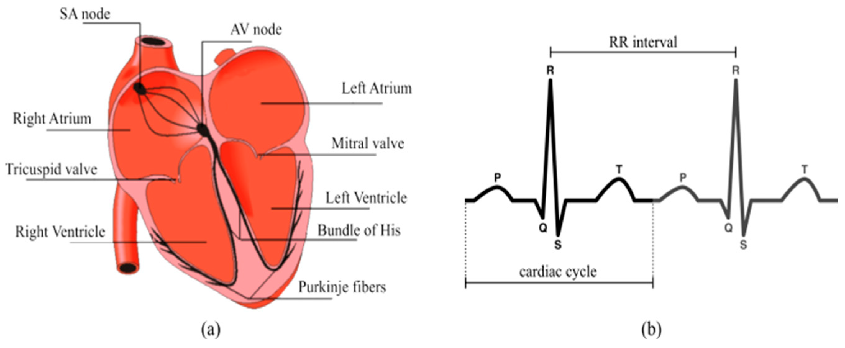
The cardiac system has the heart as the essential organ that needs to pump blood based on the electrical activity stimulus. The heart and the vascular system (Figure 1a) have the main function of ensuring continuous blood flow to the organs and tissues in order to satisfy energy needs and cellular renewal. In this regard, the cardiac conduction system ensures the normal functioning of the heart [1,2,3,4,5,6], preventing rhythm disorders or arrhythmias [7,8,9,10,11].
The electrical signals produced by the heart result from variations in intra- and extra-cellular ionic concentrations, which entrain the contraction of the two auricles and the two ventricles that constitute the heart, providing the blood circulation [12,13,14]. The cardiac dynamics have a normal functioning characterized by regular behavior in time and space. Nevertheless, they can reveal various pathologies such as tachycardia or myocardial infarction [15,16], characterized by irregular behaviors [17,18].
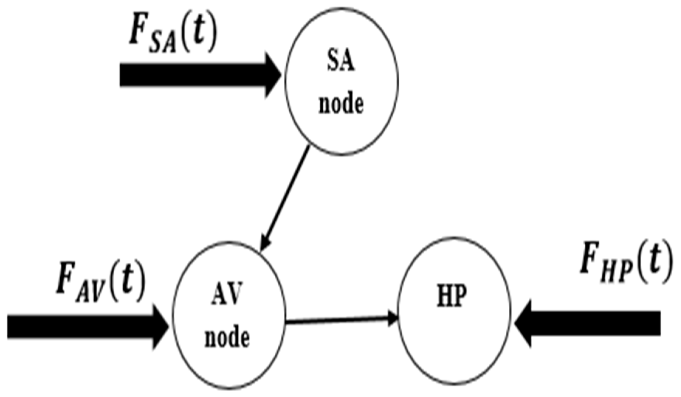
Electrical activity of the heart starts at the sinoatrial node (SA) propagates to the atrioventricular node (AV) and then to the Purkinje bundles and His–Purkinje complex (HP) Under normal functioning conditions, the sinus node generates the electrical impulse that propagate to the two atria, causing their contractions. Through the intra-atrial conduction pathways, it reaches the AV node, which after delaying it, is transmitted to the HP complex, which in turn directs it through its two branches throughout the myocardium via the Purkinje fibers [19,20]. The heart conduction system is the most plausible means of analyzing cardiac dynamics with careful study for medical interpretations [20,21,22].
The electrocardiogram (ECG) reflects electrical activity of the heart, which has the SA node as the natural pacemaker, being the most important clinical tool due to its broad use for the diagnosis of cardiac pathologies [21,22,23,24,25,26]. Electrical currents flowing through cell membranes generate electrical potentials that are responsible for cardiac muscle activity. Figure 1 shows the functional diagram of the heart and its normal ECG response characterized by three important components [2,8]: P wave, QRS complex, and T wave. The P wave represents the impulse generated by the SA node. The QRS complex is formed by ventricular contraction. The T wave reflects ventricular repolarization. Heart rate variability illustrated by the RR interval is also represented.
Mathematical modeling of the heart has been widely explored for different purposes [27,28,29,30,31]. Hodgkin and Huxley proposed the first model of electrical signal propagation through a wide variety of excitable cells around the 1950s [32] Later, FitzHugh and Nagumo provided a qualitative description of the Hodgkin–Huxley model, which led to a better understanding of its behavior [33]. They remarked that the activation of the sodium current, as well as the membrane potential, are both fast variables compared to the deactivation of the sodium current and the activation of the potassium current which are rather slow. Therefore, it simplifies a four-dimensional system to a model that is described with two variables [34,35].
Fonkou et al. [20] modified the four-equation model of FitzHugh and Nagumo to model heartbeats. A model representing the behavior of atrial tissue under fibrillation based on a finite number of hexagonal elements with five different excitability states was proposed by Moe et al. [36]. Krinsky [37] proposed a mathematical model suggesting arrhythmic causes by ignoring aspects of reintegration, vulnerability, mechanisms of initiation, development and arrest of fibrillation, “critical mass” of fibrillation, and modes of action of antiarrhythmic medications.
Many disturbances can affect the cardiac system, including physical activities, external stimuli, or breathing aspects. Several studies have been done investigating these external factors, including the work of Fonkou et al. [38,39]. It is also important to mention Krstacić et al. [40], Ernst and Bar-Joseph [41], Tobon et al. [42], Shiraishi et al. [43], Wang et al. [44], Hu et al. [45], Ueno et al. [46] and Costa and Goldberger [47].
The van der Pol (vdP) oscillator is probably the simplest model to describe the natural pacemaker defined from a reduced-order model that presents limit cycle characteristic necessary for describing the cardiac rhythm [48,49]. Following the same ideas, other models are proposed to improve the ability to describe the main aspects of the cardiac system. In this regard should be pointed out the equation by Grudzinski and Zebrowski [50] that considers modifications of the original vdP oscillator that allow a more appropriate description of the natural pacemaker. These models motivated the description of the cardiovascular system by reduced-order models that become an interesting alternative for distinct purposes. Gois and Savi [51] proposed a model with three oscillators coupled with bidirectional and asymmetrical time-delayed connections in order to obtain a representation of the ECG. Using the same approach, Cheffer et al. [2] proposed improvements to the original model by incorporating different connections. A nonlinear dynamics perspective is able to represent synthetic ECG signals, showing that a great variety of possibilities in the heart system can be explained by nonlinearities. Besides, a dynamical approach can facilitate pathology identification.
Since nonlinearities and randomness seem to be responsible for the richness of the cardiac rhythms, Cheffer and Savi [52] and Cheffer et al. [53] included non-deterministic aspects represented by random connections. The random effects allow the description of rhythm changes, explaining the transition between normal and pathological behaviors.
This article investigates the cardiac rhythm from a nonlinear dynamics perspective by considering a three-oscillator model with delayed Duffing-type connections. This model is an improvement of the model due to Cheffer et al. [2], incorporating cubic coupling terms in the governing equations that allow a broader description of pathological rhythms. In addition, a time-dependent parameter capable of inducing transient changes in cardiac rhythms is incorporated allowing the description of changes between different rhythms. In this regard, the proposed reduced-order model is able to capture the main aspects of ECGs representing normal and pathological rhythms associated with different coupling terms and transient behaviors. Numerical simulations are carried out, building synthetic ECG signals to describe the cardiac dynamics. On this basis, this work has two main novel contributions: the inclusion of delayed Duffing-type connections that allow the description of different cardiac rhythms; the inclusion of a time-dependent parameter that allows the description of transient behaviors associated with rhythm changes. Nonlinear dynamics of the heart rhythm are complex, presenting several possibilities related to pathological behavior. This complexity can include different patterns as chaotic and fractal dynamics.
After this introduction, Section 2 presents the mathematical modeling of the cardiac system. Normal synthetic ECG is analyzed in Section 3. Section 4 presents pathological synthetic ECGs, showing physiological aspects and their effects on the analysis of cardiac pathologies with and without stimuli. The frequency transition state is discussed in Section 5. Finally, the conclusions are discussed in Section 6.
2. Mathematical Modeling
Heart dynamics is essentially represented by an electrical conduction network that starts within the sinoatrial node—the natural pacemaker, located in the upper part of the inner wall of the right atrium. It emits 60 to 100 beats per minute in normal operation, being influenced by the sympathetic and parasympathetic nervous systems. The propagation of the electrical impulse from this point extends to both atria and the atrioventricular node (AV). The AV node receives the electrical signal, filters by slowing down in cases of rhythm disorders, and then directs it to the ventricles. The atrioventricular node is also influenced by the sympathetic and parasympathetic systems. The electrical impulse is then transmitted to the His bundle and Purkinje fibers. The His bundle is in the upper part of the interventricular septum and its fibers pass through the connective but non-excitable tissue that electrically separates the atria and ventricles. Finally, the electrical impulse ends up in the Purkinje network, which imposes a signal delay before leading it to the ventricular walls. The Purkinje fibers are specialized muscle fibers, allowing good electrical conduction, which ensures the simultaneous contraction of the ventricular walls. All this propagation process creates the ECG signal.
Cardiac physiology can be modeled by a reduced-order model using a system of three nonlinear oscillators with delayed connections [2,12]. External stimuli can also be incorporated to represent the space-time stimulus, promoting an increase of the reduced-order model system dimension. On this basis, any input that differs from normal functioning characterizes the stimuli, being distinct from the central nervous system activity.
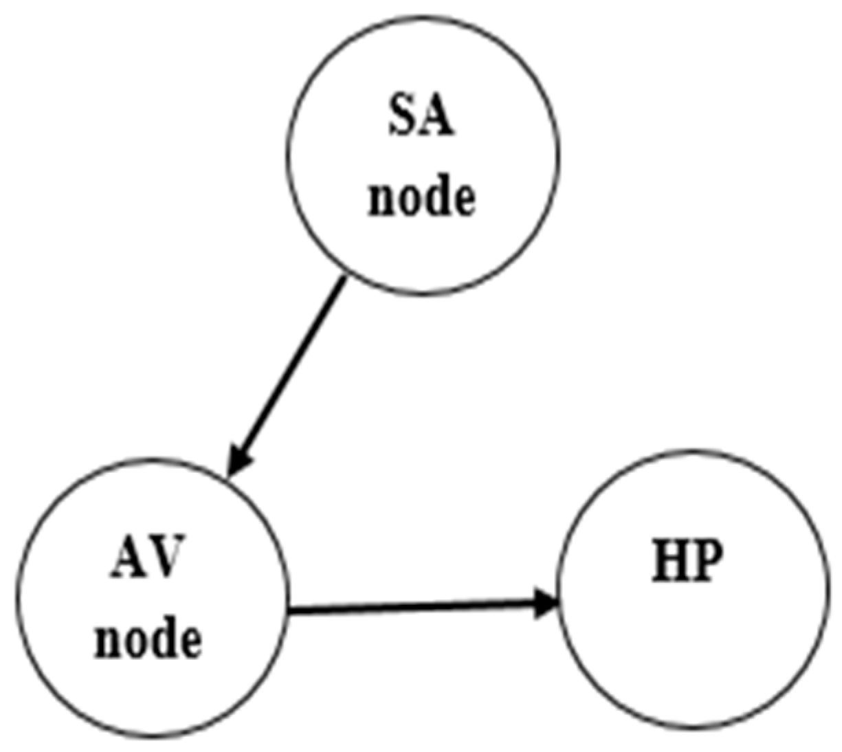
This work proposes a novel model based on the oscillator network due to Cheffer et al. [2], which is based on the original model by Gois & Savi [51]. Essentially, these models employ a three-oscillator network representing the essential nodes of the electrical activity of the heart: sinoatrial node (SA); atrioventricular node (AV); and the His–Purkinje complex (HP). Each one of these nodes is represented by the model due to Grudzinski and Zebrowski [50], which is a modification of the classical van der Pol oscillator [48,49]. This model is used in the modeling of cardiac functions since its dynamical response presents typical characteristics of biological systems such as limit cycle, synchronization, and chaos. Mathematically, its nonlinear dynamics is represented by the following differential equation,
where represents the electrical activity and the dot represents the time derivative; defines the pulse shape, characterizing the time when the heart receives the stimulus; and determine the signal amplitude, and to preserve the self-excitatory nature, ; and is an external stimulus.
The oscillator network is built by considering three oscillators coupled by Duffing-type delayed terms that include cubic nonlinearities. The coupling terms represent the propagation of the electrical pulses through the heart, being an essential aspect to describe the cardiac rhythms. A time-dependent frequency transition at the sinus node is considered in order to represent transient behaviors. In addition, external stimuli are incorporated within the model to represent other effects different from central nervous system stimuli. On this basis, the proposed model is represented by the following delayed differential equations [51]:
where represents the time delay. By considering that the indices and represent the SA, AV, or HP nodes, and and represent the coupling coefficients between nodes and , respectively, without and with delay; and are, respectively, the linear and cubic terms with delay, while and (i = 1, 2, …, 6) are, respectively, the linear and cubic terms without delay. The external excitation is given by , making the system explicitly time dependent, which increases the system dimension. Frequency transition at the sinus node is considered by assuming that the frequency parameter of the sinus node is a function of time:
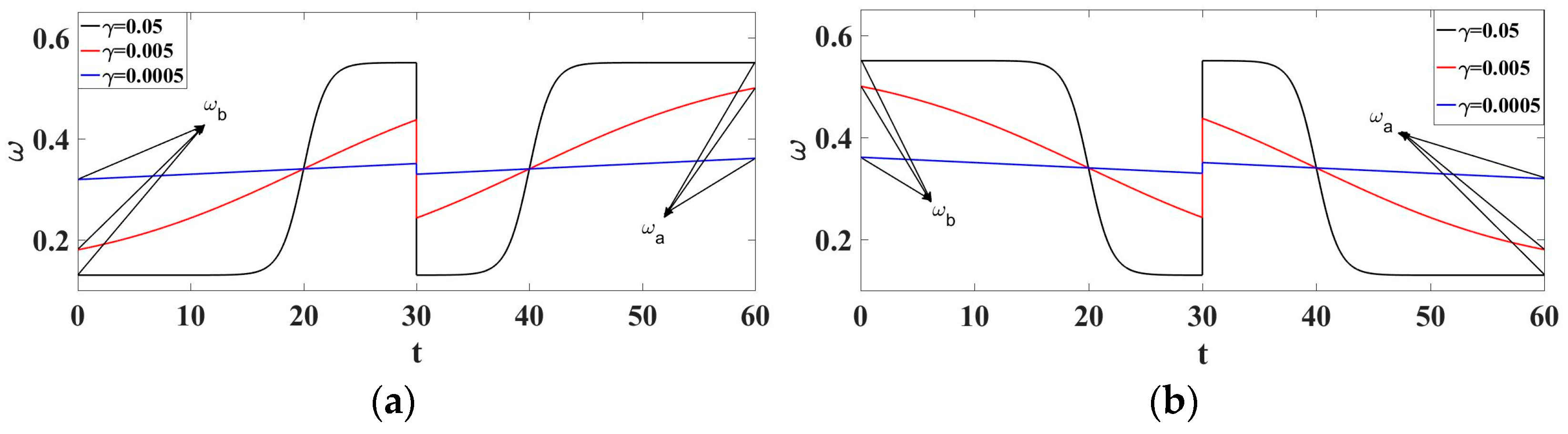
where is the transition phase between the pulsed state and the pulsed state and is the transition time. Physiologically, this frequency can represent a physical activity as well as a disturbance associated with emotional or stress. It may also indicate a defective state of the sinus node leading to transitions from normal to abnormal rhythm or transient abnormal rhythms. The dynamical behavior of this frequency is shown in Figure 2 considering three different values of . It should be noted that if .
The governing equation can be written by considering the general form,
where is the state vector and is the delayed state vector; represents the system dynamics; represents the external stimuli; represents the coupling terms while represents the delayed coupling terms.
The mathematical representation of the ECG signal can be built by the combination of the three oscillator nodes (SA, AV and HP) as follows:
where the following signals to each node are defined
with , and being constant parameters. In addition, it is possible to write:
Since the governing equations are in dimensionless form, the compliance of the dimensioning properties is observed by: where . It can be considered as the inverse of the ratio between the numerical interval and experimental interval : . Besides, the external stimuli are assumed to be harmonic: , , and . All simulations consider , , , and , and the transition phase is represented by . Besides, the initial conditions are given by: and .
3. Normal Synthetic ECG
The normal ECG can be built by considering the conceptual model with symmetrical and unidirectional connections (Figure 3). Parameters presented in Table 1 are employed to build the normal synthetic ECG, being adjusted to match experimental measurements.
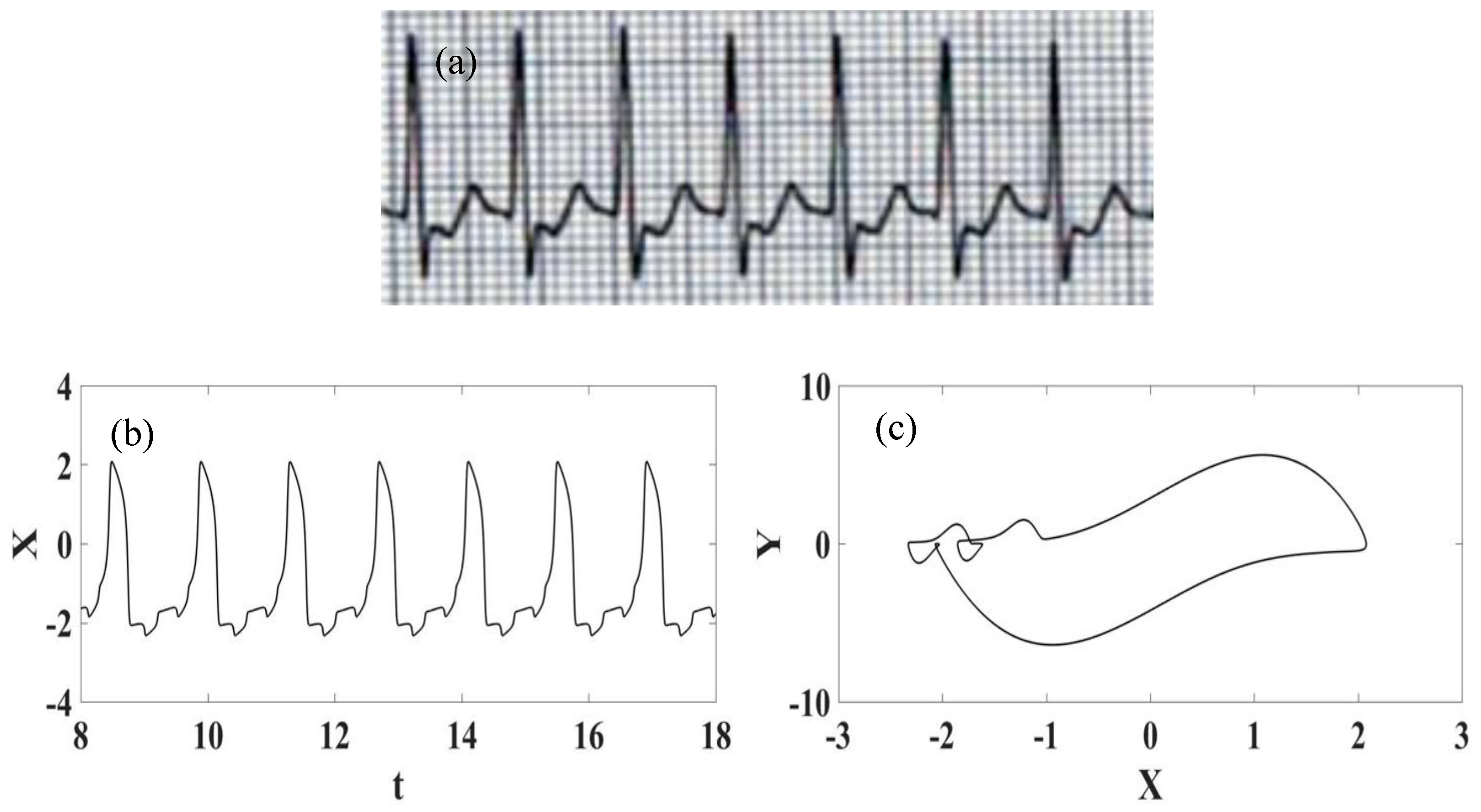
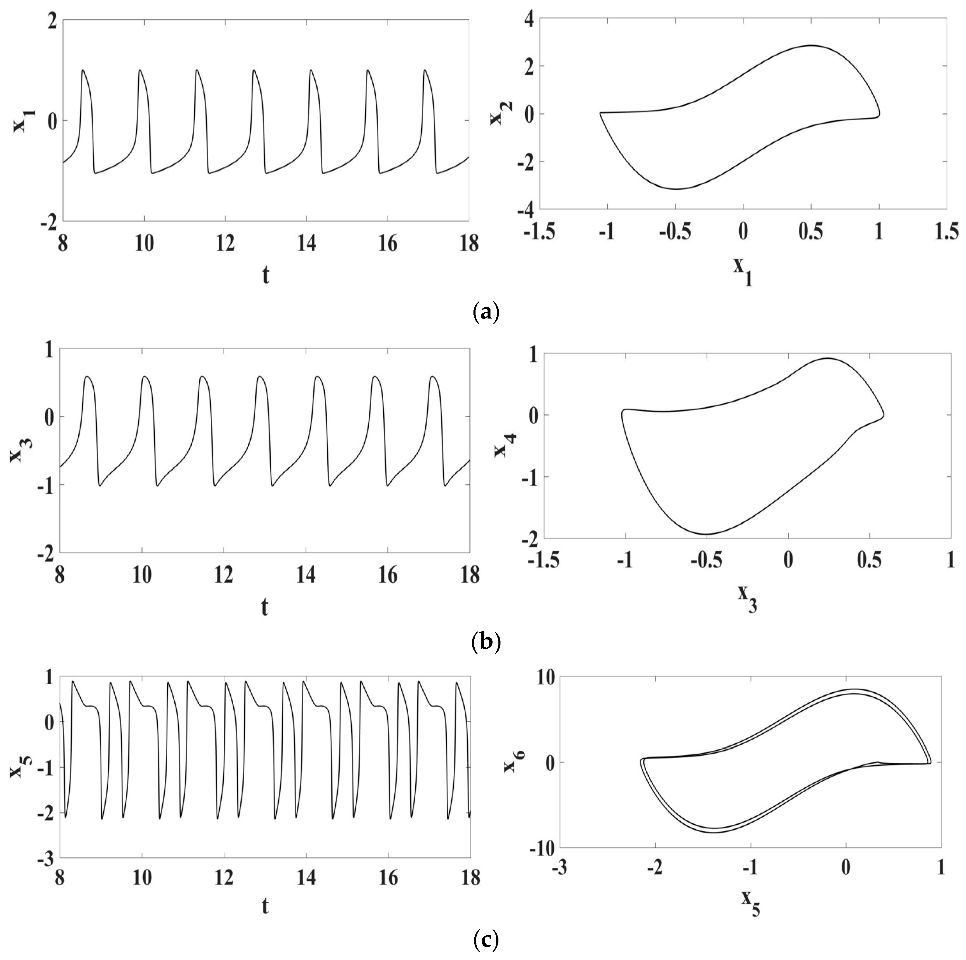
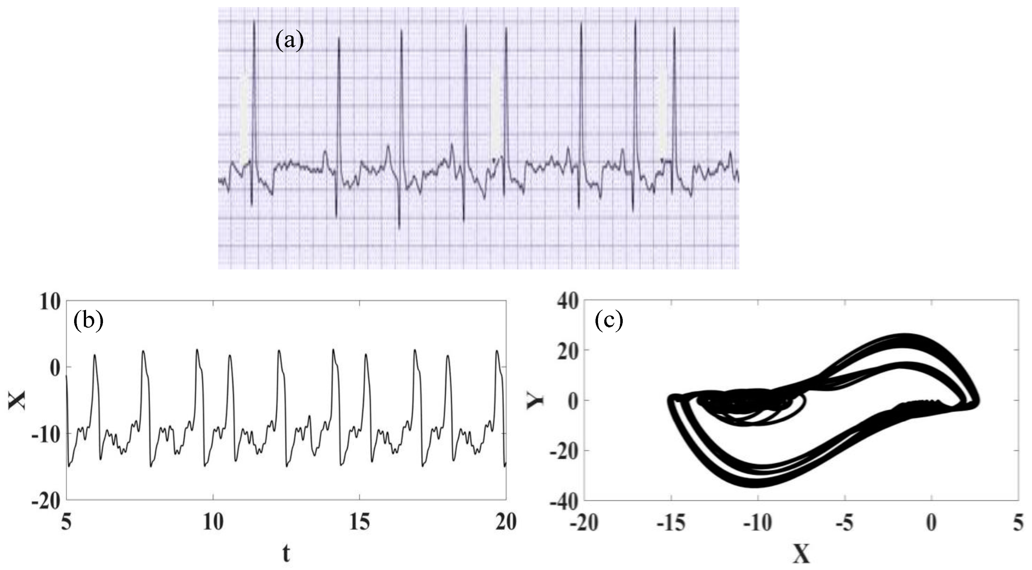
Figure 4 presents the normal synthetic ECG generated from numerical simulations establishing a comparison with the ECG signal from a real recording [54]. Note that the ECG signal presents the essential waves: P, QRS complex, and T. It should be pointed out that the synthetic ECG is a combination of each one of the three nodes that are described by nonlinear oscillators. Figure 5 presents each one of the node behaviors considering both the time series and the state space.
4. Pathological Synthetic ECGs
This section is devoted to present cardiac pathologies described from the mathematical model with different coupling characteristics. In general, irregular dynamics is related to pathological behaviors, and chaos can be identified in some of them [2]. Initially, the pathologies do not consider any external stimulus and afterward, pathologies with external stimuli are discussed. Situations without external stimulus are related to the following pathological rhythms: ventricular flutter, torsade de pointes, atrial flutter, and atrial fibrillation. By considering external stimuli, the pathological rhythms captured are the following: ventricular fibrillation, polymorphic ventricular tachycardia, and supraventricular extrasystole. Table 2 summarizes the employed parameters for numerical simulations, adjusted from experimental measurements. It should be pointed out that all pathologies discussed by Cheffer et al. [2] can also be reproduced by the current form of the model.
4.1. Ventricular Flutter
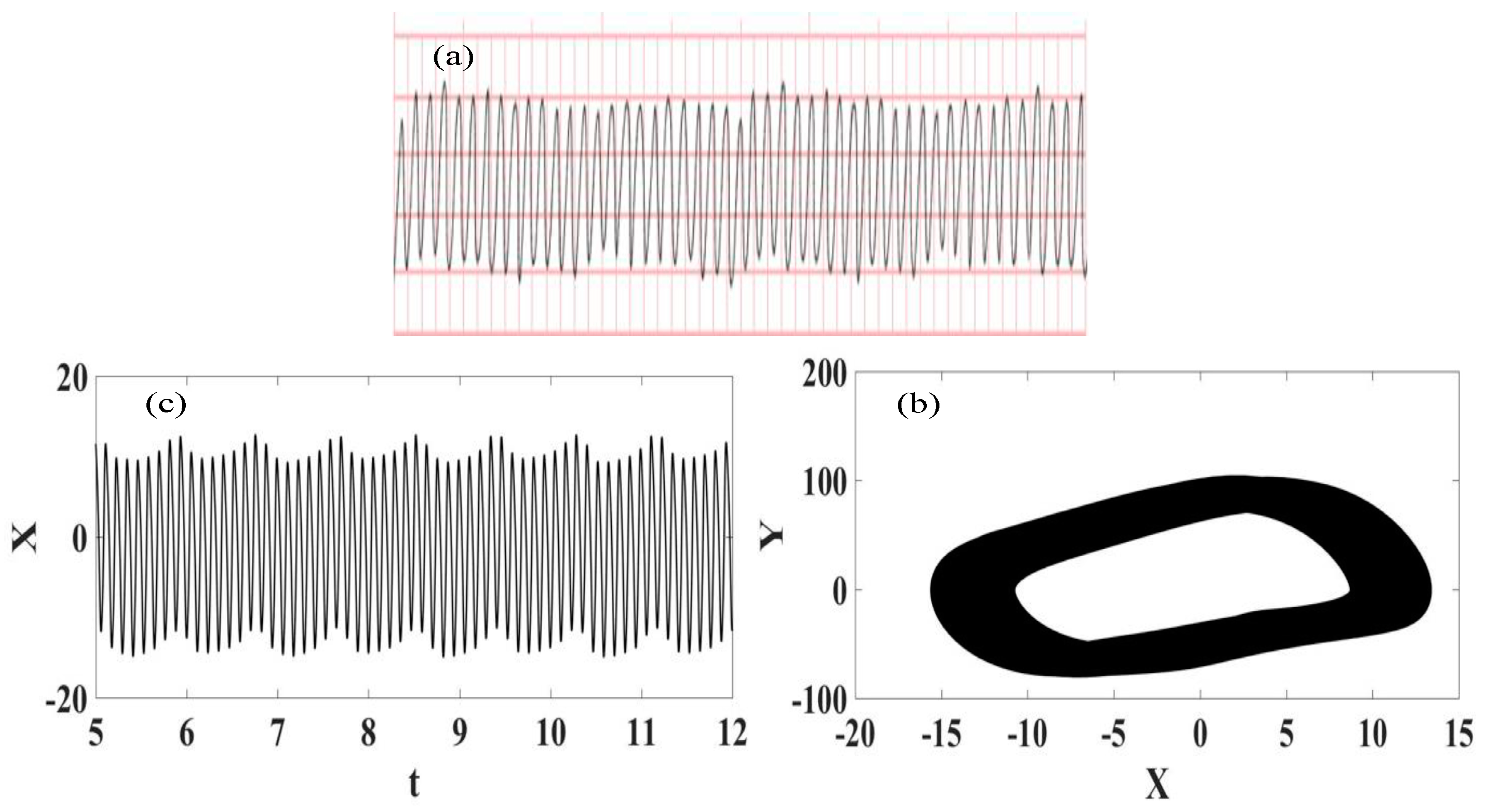
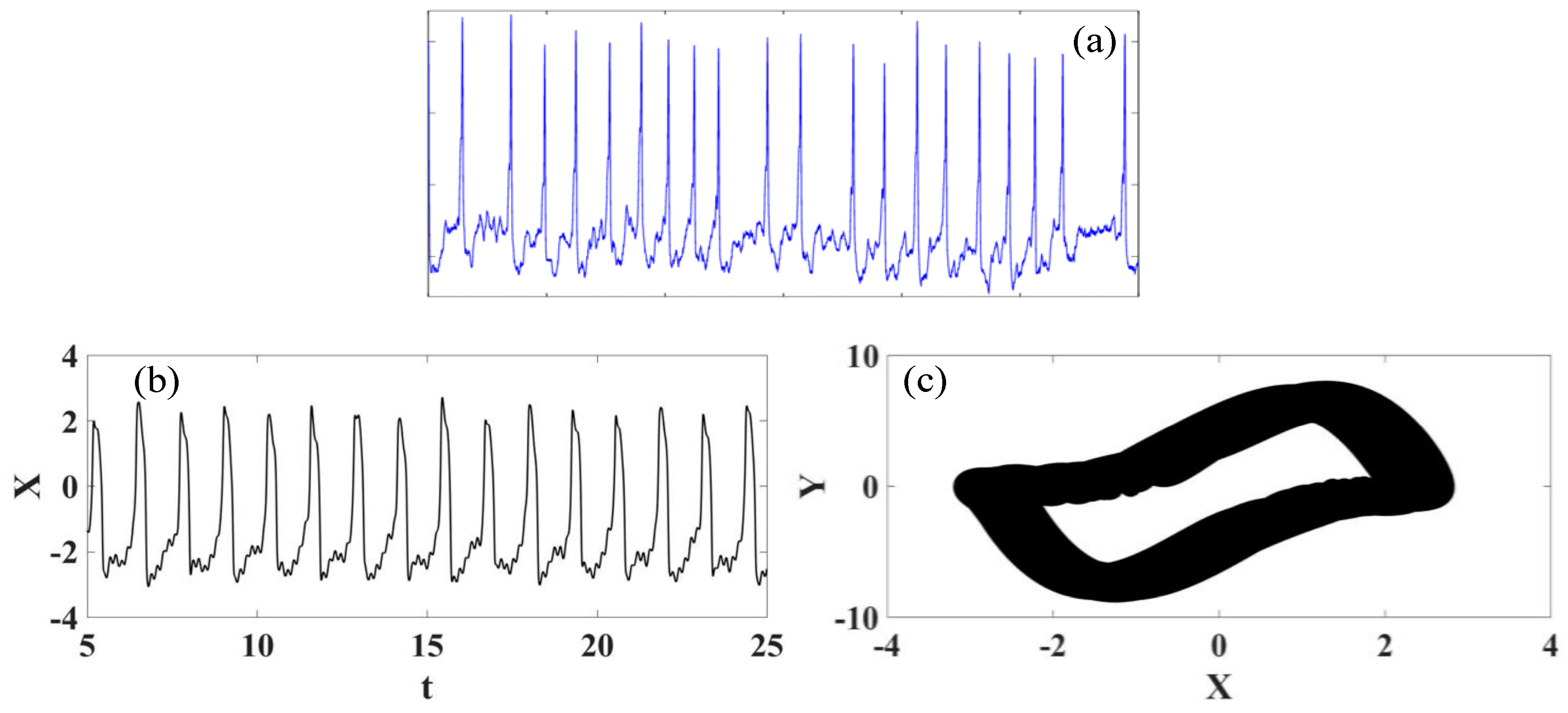
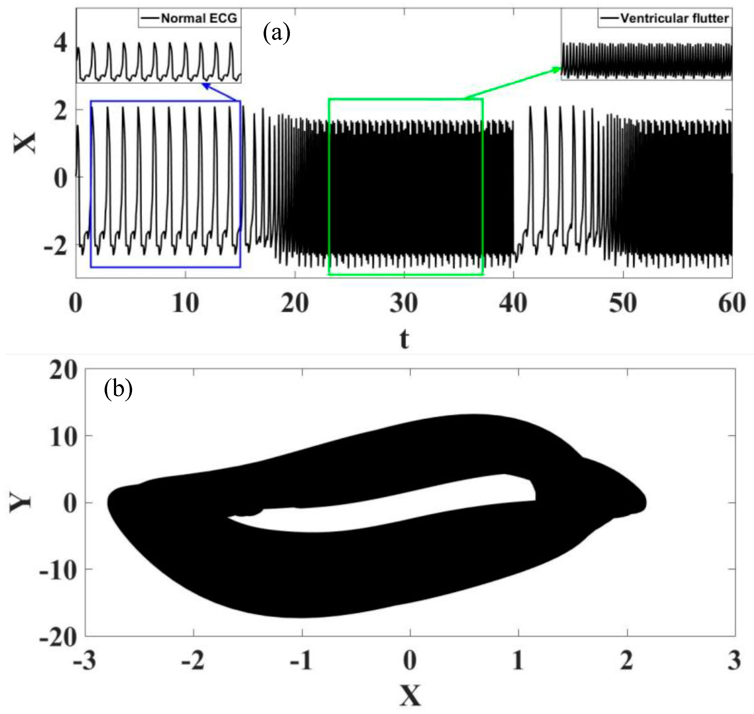
Ventricular flutter is a tachycardia affecting the ventricles with a rate greater than 250–350 beats per minute [55]. The ECG is characterized by a sinusoidal waveform with no clear definition of QRS complex and T wave. It can stop on its own, being possible to be related to loss of consciousness without being fatal. Nevertheless, it can be a transitional stage to either ventricular tachycardia or fibrillation, which are more critical arrythmia. Ventricular flutter can be associated with genetic heart diseases called channelopathies, including the “long QT syndrome” or LQTS. Figure 6 presents the synthetic ECG signal compared with the real ECG one [56]. It is noticeable that the ECG signal has a high number of beats per minute and good agreement between numerical and real data.
4.2. Torsade de Pointe (TdP)
Torsade de Pointe (TdP) is a specific form of polymorphic ventricular tachycardia (PVT) occurring in the context of QT interval prolongation. This arrythmia has a morphology in which the QRS complex twists around the isoelectric line [58]. The diagnosis of the TdP is related to the evidence of PVT and QT prolongation. TdP is often short-lived and self-limiting, being associated with hemodynamic instability and collapse. It may also degenerate into ventricular fibrillation. Physiologically, a prolonged QT reflects on longer myocyte repolarization due to ion channel dysfunction, which also gives rise to early depolarizations (ADEs) that can manifest on the ECG as high U waves; if these reach a threshold amplitude, they can manifest as premature ventricular contractions (PVCs). TdP is initiated when a PVC occurs during the preceding T wave, known as the “R on T” phenomenon. The onset of TdP is often preceded by a sequence of short-long-short RR intervals, known as “pause-dependent” TDPs, with longer pauses associated with more rapid executions of TdP. The ECG signal that characterizes the TdP pathology is presented in Figure 7 [57] together with numerical simulations represented by ECG signal and phase space. The comparison between numerical and real data shows good agreement.
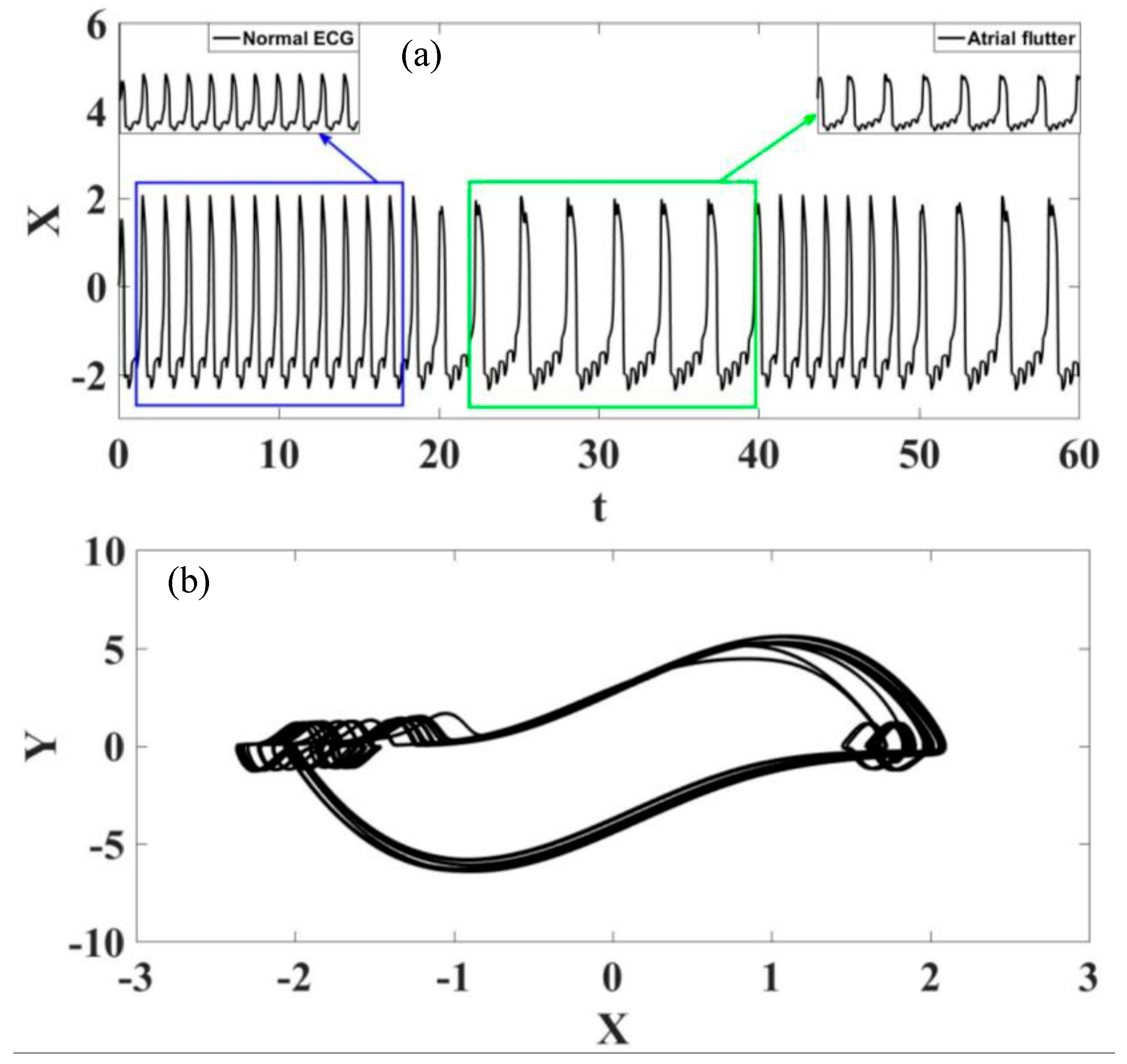
4.3. Atrial Flutter
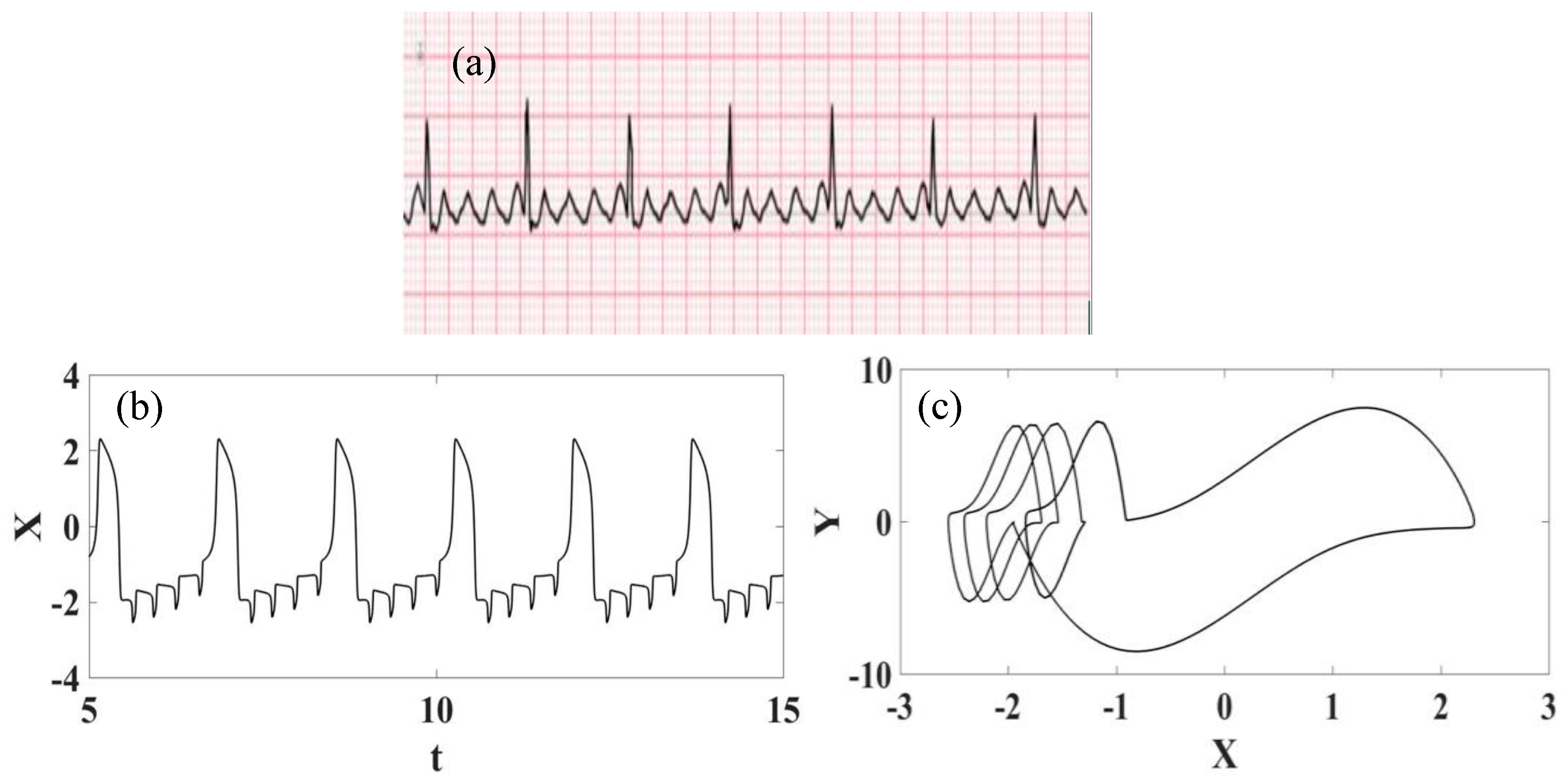
Atrial flutter is a regular rapid rhythm of the atria associated with ECGs with a sawtooth conduction pattern [59]. The heart rates are around 150 beats per minute, but sometimes the rates may be slower. This pathology can cause progressive heart failure (weakness of the heart muscle), so symptoms that may persist include shortness of breath, chest pain, fatigue, dizziness, and palpitations. This risk is particularly high if the heart rates in atrial flutter are constantly around 150 bpm. A typical atrial flutter real ECG is presented in Figure 8 [57] together with synthetic time series and phase space. It is noticeable that there is qualitative good agreement between the numerical and experimental data.
4.4. Atrial Fibrillation
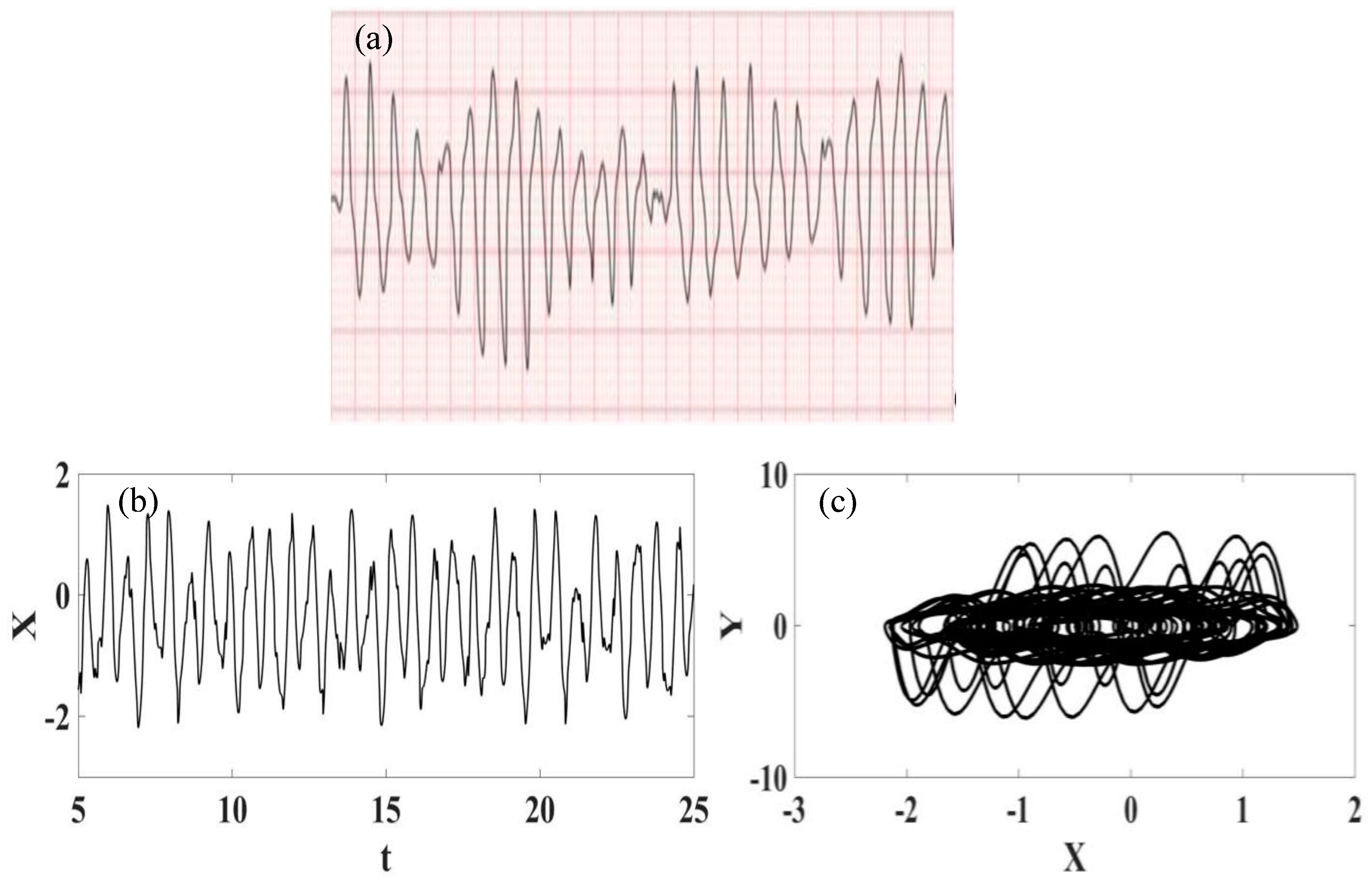
Atrial fibrillation (AF) is a heart condition that causes an irregular and often abnormally fast heart rhythm, being the most diagnosed arrhythmia [60]. In contrast with the normal heart rhythm, which stays between 60 and 100 beats per minute at rest, atrial fibrillation can present a heart rate higher than 140 beats per minute with an irregularity that often causes poor blood flow in the body. Atrial fibrillation occurs when abnormal electrical impulses suddenly occur in the atria, replacing the natural pacemaker that can no longer control the heartbeat, causing irregular pulses. The high-rate rhythm usually makes the heart muscle unable to relax properly between contractions, reducing the efficiency and performance of the heart. Figure 9 presents the atrial flutter ECG signal obtained from real recording [57] and synthetic ECGs. Note the irregular and abnormally fast heart rhythm and that, once again, it is possible to observe a good agreement between numerical and experimental data.
4.5. Ventricular Fibrillation
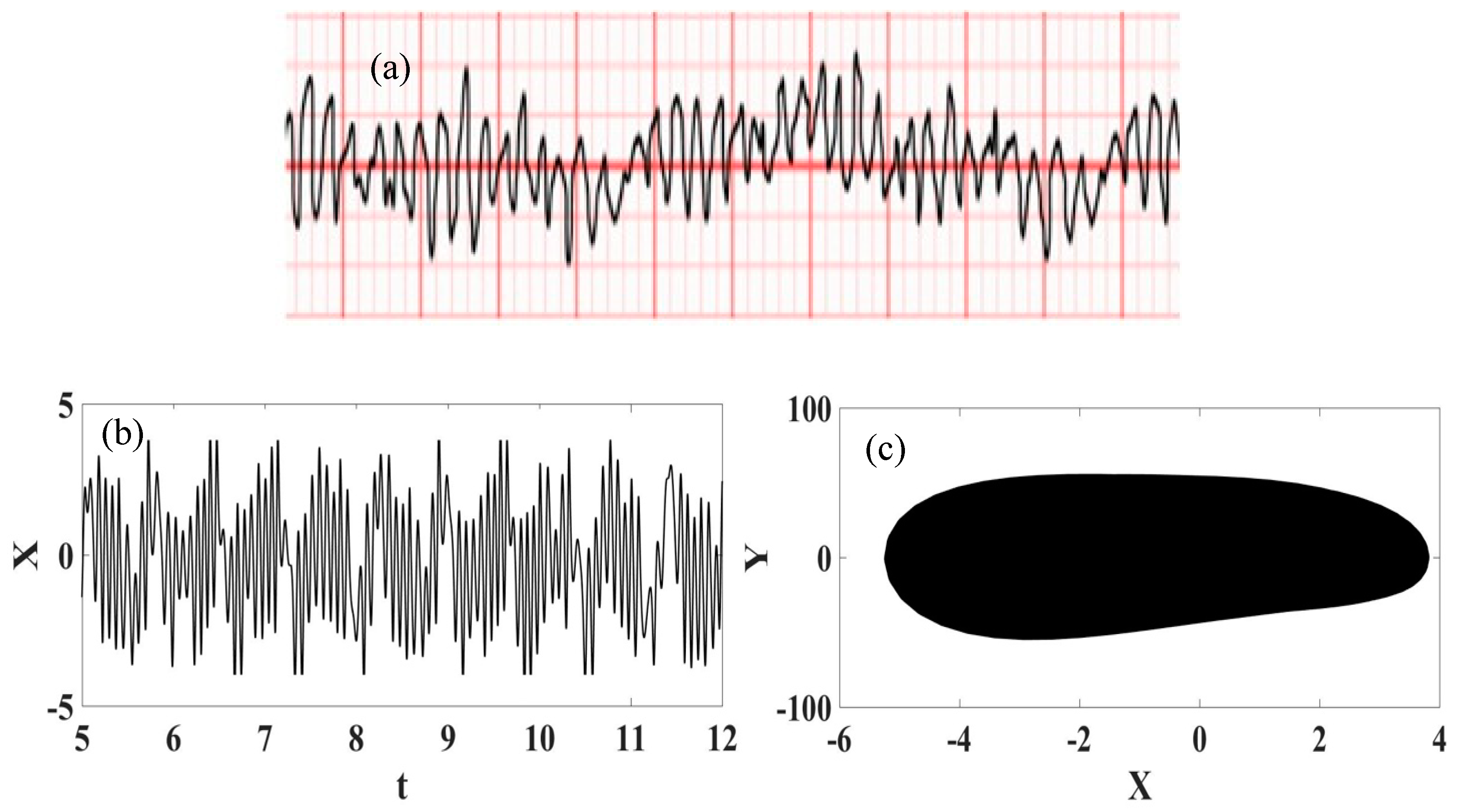
Ventricular fibrillation (VF) is an acute life-threatening, tachycardic arrhythmia of the heart in which the ventricular rate is greatly increased (over 320 beats per minute). During ventricular fibrillation, the transmission of electrical impulses from the heart is disturbed and the muscle fibers contract in a disordered manner, which makes the body’s blood supply no longer guaranteed [61]. It usually causes a rapid consciousness loss, being responsible for most sudden deaths during the acute phase of the infarction (over 70%), and also leading to other arrhythmias (over 80%). Many factors can cause the onset of ventricular fibrillation such as: coronary disease, myocardial infarction, heart failure, myocarditis, high blood pressure, and certain congenital heart defects.
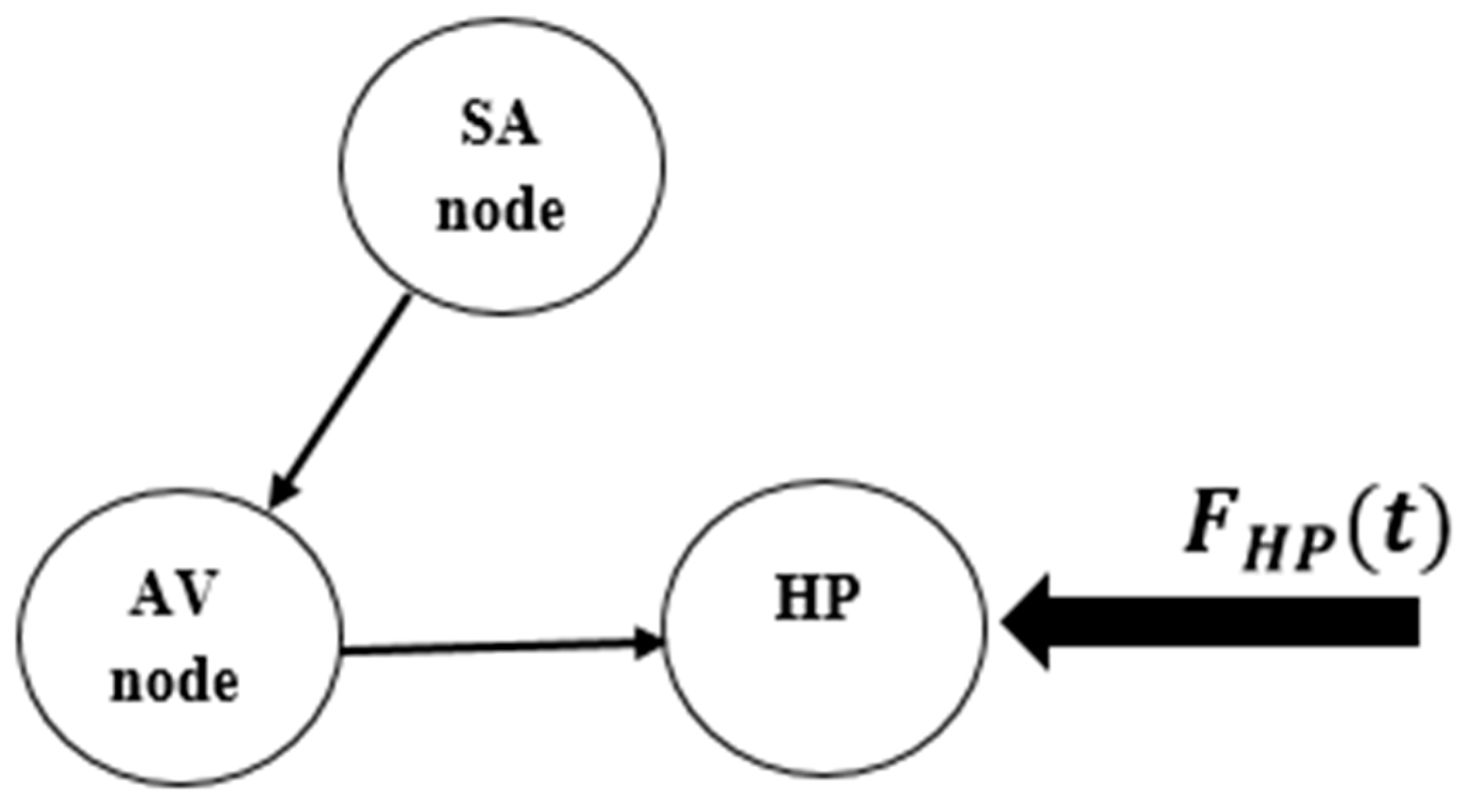
Ventricular fibrillation can be represented by considering the conceptual model of the heart functioning presented in Figure 10, where an external stimulus is of concern. The dynamical rhythm is presented in Figure 11, showing the experimental ECG [57] together with synthetic ECG time series and phase space. The good agreement between them should be pointed out.
4.6. Polymorphic Ventricular Tachycardia
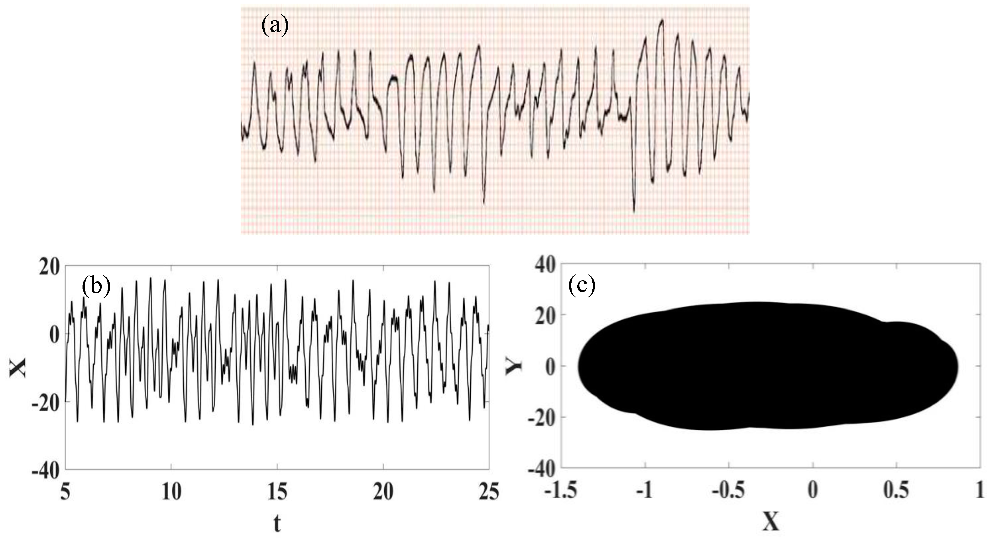
Polymorphic ventricular tachycardia (PVT) is a condition that includes a wide range of other conditions, such as, for instance, torsade de pointes, bidirectional ventricular tachycardia, and other types of ventricular tachycardia with variable morphologies [62]. It can be induced by catecholamines or stress testing, but some children without apparent heart disease may also develop it. PVT is part of a myriad of supraventricular and ventricular arrhythmias occurring sequentially, including various types of polymorphic ventricular tachycardias, such as bursts of bidirectional ventricular tachycardia. Polymorphic ventricular tachycardias may show intermediate or atypical morphologies when they develop into a flutter. Sometimes, QRS morphologies change over time.
The ECG real recording of polymorphic ventricular tachycardia is presented in Figure 12 together with synthetic ECG presented in the form of time series and phase space. Once again, a qualitative good agreement is observed.
4.7. Supraventricular Extrasystole
Supraventricular extrasystoles (SVEs) are premature contractions that originate in the atrial or junctional tissue (at the atrioventricular junction) [56]. In the basic sinus rhythm, the SVE appears as a premature P-QRS-T sequence. The P wave presents a morphology that is often different from that of the sinus P wave and can be positive or negative due to the fact that the atria are depolarized in an abnormal pathway. Moreover, the P wave can merge with the T wave of the preceding complex. The QRS complex and T wave are basically identical to those of sinus sequences (morphology at least 90% similar), except in the case of early extrasystole on rapid tachycardia (sinus or not), called ventricular aberration.
The supraventricular extrasystole can be represented by the conceptual model presented in Figure 13, where external stimuli are assumed. ECG real signal and synthetic ECG are presented in Figure 14, considering time series and phase space. Noticeable are irregularities related to premature contractions, and a good agreement between real data and numerical simulations.
5. Frequency Transition State
The SA node is the natural pacemaker and disturbances in its functioning induces changes in the cardiac rhythm. In this regard, the parameter can represent these changes, describing transient effects responsible for the variations between different rhythms. This section treats some situations that illustrate the ability of this parameter to represent transition regimes. Table 3 illustrates parameters that are employed to represent four different situations: transition between normal rhythm and atrial flutter; transition between normal rhythm and ventricular flutter; transition between ventricular fibrillation and normal rhythm; transition between ventricular tachycardia and normal rhythm. These results point to the transient behavior of the SA node generating transient behaviors that appear in ECG signals.
Initially, the transition from normal rhythm to atrial flutter is of concern. Figure 15 shows ECGs represented by time series and state space. Both behaviors are highlighted in the zoomed-in details, and noticeable is an alternation between different dynamical patterns describing the behavior of atrial flutter (as presented in Figure 8) and dynamics characterizing the behavior of a normal ECG. Details depicted in Figure 15 help the identification of these behaviors.
The transition from normal rhythm to ventricular flutter is now in focus and Figure 16 presents these transitions in the form of time series and phase space. Once again, it is possible to identify different transition regimes, now changing from normal to ventricular flutter rhythms.
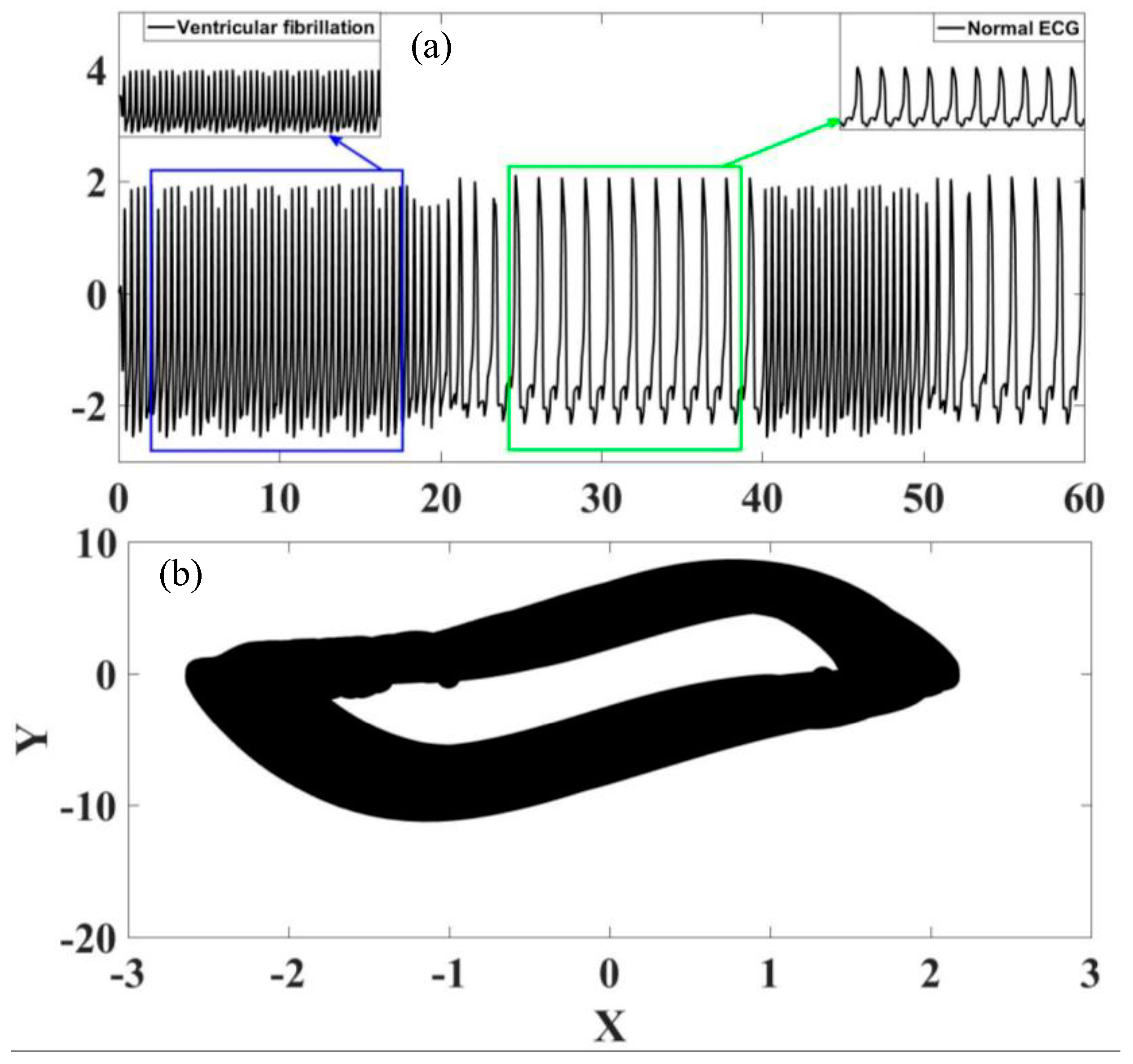
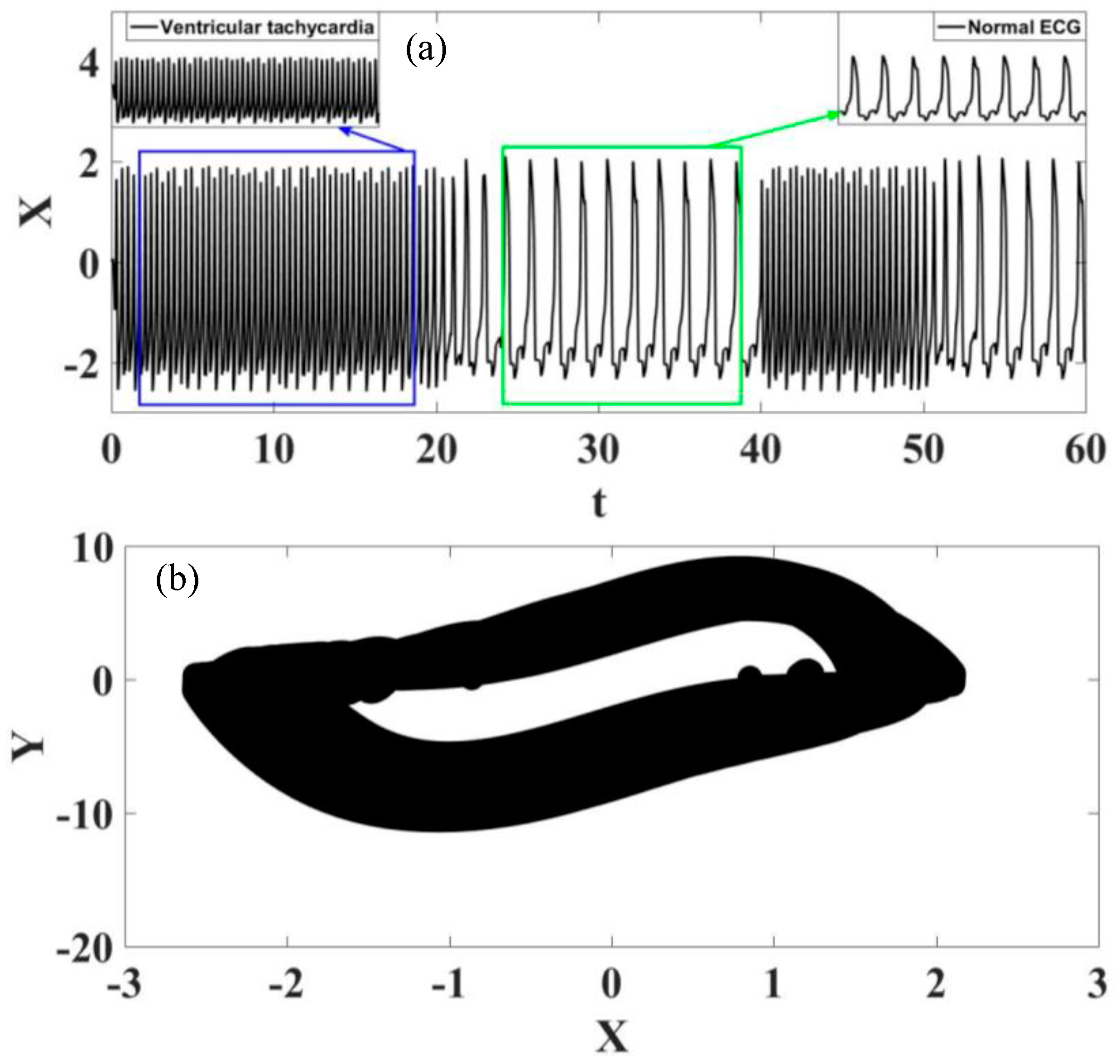
Figure 17 shows the analysis of the transition from ventricular fibrillation to normal rhythm. The observation of this case is different from those observed in the previous situations because the transition starts from a pathological rhythm, changing to a normal rhythm. On the other hand, Figure 18 presents a transition from ventricular tachycardia, characterized by rapid heartbeat, to normal rhythm. Based on these results, it is possible to conclude that transition regimes can be properly described by the sinoatrial node time dependent parameter.
6. Conclusions
This work deals with cardiac rhythms analyzed from a nonlinear dynamics perspective considering a three-oscillator model with Duffing-type delayed connections. In addition, transient behavior is represented by a sinoatrial node time-dependent parameter. The model is capable of representing a wide variety of responses, including normal and pathological rhythms characterized by ECG signals. Numerical simulations show the following rhythms: normal rhythm, ventricular flutter, torsade de pointe, atrial flutter, atrial fibrillation, ventricular fibrillation, polymorphic ventricular tachycardia, and supraventricular extrasystole. In addition, although it is not presented in this paper, all the pathologies discussed in Cheffer et al. [2] have been represented. The transient behavior of the sinoatrial node shows that transitions from normal to pathological rhythms are properly represented. In this regard, the following transient behaviors are identified: transition from normal rhythm to atrial flutter; transition from normal rhythm to ventricular flutter; transition from ventricular fibrillation to normal rhythm; transition from ventricular tachycardia to normal rhythm. On this basis, a Duffing-type connection seems to be an interesting approach to enhance the cardiac description and time-dependent parameters, allowing a proper description of transient behaviors among different heart rhythms. The broad variety of rhythms described by the reduced-order mathematical model encourages its use in different situations such as rhythm identification, artificial pacemakers, and controller design. Besides, the nonlinear dynamics perspective seems to be essential for the correct comprehension of the cardiac system behavior, being useful to classify and identify pathological behavior.
Author Contributions
Conceptualization, R.F.F. and M.A.S.; methodology, R.F.F. and M.A.S.; software, R.F.F.; validation, R.F.F. and M.A.S.; formal analysis, R.F.F. and M.A.S.; investigation, R.F.F. and M.A.S.; resources, R.F.F. and M.A.S.; writing—original draft preparation, R.F.F. and M.A.S.; writing—review and editing, R.F.F. and M.A.S.; visualization, R.F.F. and M.A.S.; supervision, M.A.S.; project administration, M.A.S.; funding acquisition, M.A.S. All authors have read and agreed to the published version of the manuscript.
Funding
The authors would like to acknowledge the support of the Brazilian Research Agencies CNPq (301.350/2018-3) CAPES (Proex 23038007615-2021-78), and FAPERJ (E-26/201.017/2022).
Data Availability Statement
The datasets are available from the corresponding author on reasonable request.
Conflicts of Interest
The authors declare no conflict of interest.
References
- Nazari, S.; Heydari, A.; Khaligh, J. Modified modeling of the heart by applying nonlinear oscillators and designing an appropriate control signal. Appl. Math. 2013, 4, 972–978. [Google Scholar] [CrossRef] [Green Version]
- Cheffer, A.; Savi, M.A.; Pereira, T.L.; de Paula, A.S. Heart rhythm analysis using a nonlinear dynamics perspective. Appl. Math. Model. 2021, 96, 152–176. [Google Scholar] [CrossRef]
- Fonkou, R.F.; Kengne, R.; Fotsing Kamgang, H.C.; Talla, P.K. Dynamical behavior analysis of the heart system by the bifurcation structures. Heliyon 2023, 9, e12887. [Google Scholar] [CrossRef] [PubMed]
- Cheffer, A.; Savi, M.A. Analysis of Cardiovascular Rhythms Using Mathematical Models. J. Cardiovasc. Med. 2021, 5, 022. [Google Scholar]
- La Sala, L.; Crestani, M.; Garavelli, S.; de Candia, P.; Pontiroli, A.E. Does microRNA disruption control the mechanisms linking obesity and diabetes? Implications for cardiovascular risk. Int. J. Mol. Sci. 2021, 22, 143. [Google Scholar] [CrossRef]
- Britin, S.N.; Britina, M.A.; Vlasenko, R.Y. Cardiac Conduction System: A Generalized Electrical Model. Biomed. 2021, 55, 41–45. [Google Scholar] [CrossRef]
- Savi, M.A. Chaos and order in biomedical rhythms. J. Braz. Soc. Mech. Sci. Eng. 2005, 27, 157–169. [Google Scholar] [CrossRef] [Green Version]
- Cheffer, A.; Savi, M.A. Biochaos in Cardiac Rhythms. Eur. Phys. J. Spec. Top. 2022, 231, 833–8455. [Google Scholar] [CrossRef]
- Ferreira, B.B.; Savi, M.A.; De Paula, A.S. Chaos control applied to cardiac rhythms represented by ECG signals. Phys. Scr. 2014, 89, 105203. [Google Scholar] [CrossRef]
- Baleanu, D.; Sajjadi, S.S.; Asad, J.H.; Jajarmi, A.; Estiri, E. Hyperchaotic behaviors, optimal control and synchronization of a non-autonomous cardiac conduction system. Adv. Differ. Equ. 2021, 2021, 157. [Google Scholar] [CrossRef]
- De Almeida, M.C.; Shumpei Mori, S.; Anderson, R.H. Three-dimensional visualization of the bovine cardiac conduction system and surrounding structures compared with arrangements in the human heart. J. Anat. 2021, 238, 1359–1370. [Google Scholar] [CrossRef]
- Adrian, E.D.; Bronk, D.W. Discharges in mammalian sympathetic nerves. J. Physiol. 1932, 2, 115–133. [Google Scholar] [CrossRef] [PubMed]
- Park, D.S.; Fishman, G.I. The cardiac conduction system. Circulation 2011, 8, 904–915. [Google Scholar] [CrossRef] [Green Version]
- Poon, C.-S.; Barahona, M. Titration of chaos with added noise. Proc. Natl. Acad. Sci. USA 2001, 98, 7107–7112. [Google Scholar] [CrossRef] [PubMed]
- Radhakrishna, R.K.A.; Dutt, D.N.; Yeragan, V.K. Nonlinear measures of heart rate time series: Influence of posture and controlled breathing. Auton. Neurosci. Basic Clin. 2000, 83, 148–158. [Google Scholar] [CrossRef] [PubMed]
- Van der Schouw, Y.T.; Van der Graaf, Y.; Steyerberg, E.W.; Eijkemans, M.J.C.; Banga, J.D. Age at menopause as a risk factor for cardiovascular mortality. Lancet 1996, 347, 714–718. [Google Scholar] [CrossRef] [Green Version]
- Venkat Narayan, K.M.; Thompson, T.J.; Boyle, J.P.; Beckles, G.L.A.; Engelgau, M.M.; Vinicor, F.; Williamson, D.F. The use of population attributable risk to estimate the impact of prevention and early detection of type 2 diabetes on population-wide mortality risk in US males. Health Care Manag. Sci. 1999, 2, 223–227. [Google Scholar] [CrossRef]
- Wåhlin, A.; Nyberg, L. At the Heart of Cognitive Functioning in Aging. Trends Cogn. Sci. 2019, 23, 717–720. [Google Scholar] [CrossRef]
- Santos, A.M.; Lopes, S.R.; Viana, R.L. Rhythm synchronization and chaotic modulation of coupled Van der Pol oscillators in a model for the heartbeat. Phys. A 2004, 338, 335–355. [Google Scholar] [CrossRef]
- Fonkou, R.F.; Louodop, P.; Talla, P.K. Dynamic behaviour of the cardiac conduction system under external disturbances: Simulation based on microcontroller technology. Phys. Scr. 2022, 97, 025001. [Google Scholar] [CrossRef]
- Richter, Y.; Edelman, E.R. Cardiology Is Flow. Circulation 2006, 113, 2679–2682. [Google Scholar] [CrossRef] [PubMed] [Green Version]
- Kik, M.J.L.; Path, D.V.; Mitchell, M.A. Reptile cardiology: A review of anatomy and physiology, diagnostic approaches, and clinical disease. Semin. Avian Exot. Pet Med. 2005, 14, 52–60. [Google Scholar] [CrossRef] [Green Version]
- Plonsey, R.; Barr, R.C. Mathematical modeling of electrical activity of the heart. J. Electrocardiol. 1987, 20, 219–226. [Google Scholar] [CrossRef]
- Banerjee, A.; Newman, D.R.; Van den Bruel, A.; Heneghan, C. Diagnostic accuracy of exercise stress testing for coronary artery disease: A systematic review and meta-analysis of prospective studies. Int. J. Clin. Pract. 2012, 66, 477–492. [Google Scholar] [CrossRef]
- Wiener, D.A.; Ryan, T.J.; McCabe, C.H.; Ward Kennedy, J.; Schloss, M.; Tristani, F.; Chaitman, B.R.; Fisher, L.D. Exercise Stress Testing—Correlations among History of Angina, ST-Segment Response and Prevalence of Coronary-Artery Disease in the Coronary Artery Surgery Study (CASS). N. Engl. J. Med. 1979, 301, 230–235. [Google Scholar] [CrossRef]
- Bonow, R.O.; Carabello, B.A.; Chatterjee, K.; de Leon, A.C., Jr.; Faxon, D.P.; Freed, M.D.; Gaasch, W.H.; Lytle, B.W.; Nishimura, R.A.; O’Gara, P.T.; et al. 2008 Focused Update Incorporated Into the ACC/AHA 2006 Guidelines for the Management of Patients With Valvular Heart Disease. Circulation 2008, 118, e523–e661. [Google Scholar] [CrossRef] [Green Version]
- Fonkou, R.F.; Louodop, P.; Talla, P.K. Nonlinear oscillators with variable state damping and elastic coefficients. Pramana J. Phys. 2021, 95, 210. [Google Scholar] [CrossRef]
- Bozkurt, S. Mathematical modeling of cardiac function to evaluate clinical cases in adults and children. PLoS ONE 2019, 14, e0224663. [Google Scholar] [CrossRef]
- Barrio, R.; Shilnikov, A. Parameter-sweeping techniques for temporal dynamics of neuronal systems: Case study of Hindmarsh-Rose model. J. Math. Neurosci. 2011, 1, 6. [Google Scholar] [CrossRef] [Green Version]
- Traver, J.E.; Nuevo-Gallardo, C.; Tejado, I.; Fernández-Portales, J.; Ortega-Morán, J.F.; Pagador, J.B.; Vinagre, B.M. Cardiovascular Circulatory System and Left Carotid Model: A Fractional Approach to Disease Modeling. Fractal Fract. 2022, 6, 64. [Google Scholar] [CrossRef]
- Suchorsky, M.; Rand, R. Three Oscillator of the heartbeat generator. Commun. Nonlinear Sci. Numer. Simul. 2009, 14, 2434–2449. [Google Scholar] [CrossRef]
- Hodgkin, A.L.; Huxley, A.F. A quantitative description of membrane current and its application to conduction and excitation in nerve. J. Physiol. 1952, 117, 500–544. [Google Scholar] [CrossRef] [PubMed]
- FitzHugh, R. Impulses and physiological states in theorical models of nerve membrane. Biophys. J. 1961, 1, 445–466. [Google Scholar] [CrossRef] [Green Version]
- Nagumo, J.; Arimoto, S.; Yoshizawa, S. An active pulse transmission line simulating nerve axon. Proc. IRE 1962, 50, 2061–2070. [Google Scholar] [CrossRef]
- Kuate, G.C.G.; Fotsin, H.B. On the nonlinear dynamics of a cardiac electrical conduction system model: Theoretical and experimental study. Phys. Scr. 2022, 97, 045205. [Google Scholar] [CrossRef]
- Moe, G.K.; Rheinboldt, W.C.; Abildskov, J.A. A computer model of atrial fibrillation. Am. Heart J. 1964, 67, 200–220. [Google Scholar] [CrossRef]
- Krinsky, V.I. Mathematical models of cardiac arrhythmias (spiral waves). Pharmacol. Ther. Part B 1978, 3, 539–555. [Google Scholar] [CrossRef]
- Fonkou, R.F.; Louodop, P.; Talla, P.K.; Woafo, P. Analysis of the dynamics of new models of nonlinear systems with state variable damping and elastic coefficients. Heliyon 2022, 8, e10112. [Google Scholar] [CrossRef]
- Fonkou, R.F.; Louodop, P.; Talla, P.K.; Woafo, P. Van der Pol equation with sinusoidal nonlinearity: Dynamic behaviour and real-time control of a target trajectory. Phys. Scr. 2021, 96, 125203. [Google Scholar] [CrossRef]
- Krstacic, G.; Krstacic, A.; Smalcelj, A.; Milicic, D.; Jembrek-Gostovic, M. The chaos theory and nonlinear dynamics in heart rate variability analysis: Does it work in short-time series in patients with coronary heart disease? Ann. Noninvasive Electrocardiol. 2007, 12, 130–136. [Google Scholar] [CrossRef]
- Ernst, J.; Bar-Joseph, Z. STEM: A tool for the analysis of short time series gene expression data. BMC Bioinform. 2006, 7, 1–11. [Google Scholar] [CrossRef] [PubMed] [Green Version]
- Tobón, D.P.; Jayaraman, S.; Falk, T.H. Spectro-temporal electrocardiogram analysis for noise-robust heart rate and heart rate variability measurement. IEEE J. Transl. Eng. Health Med. 2017, 5, 1–11. [Google Scholar] [CrossRef] [PubMed]
- Shiraishi, Y.; Katsumata, Y.; Sadahiro, T.; Azuma, K.; Akita, K.; Isobe, S.; Yashima, F.; Miyamoto, K.; Nishiyama, T.; Tamura, Y.; et al. Real-time analysis of the heart rate variability during incremental exercise for the detection of the ventilatory threshold. J. Am. Heart Assoc. 2018, 7, e006612. [Google Scholar] [CrossRef] [Green Version]
- Wang, Y.; Wei, S.; Zhang, S.; Zhang, Y.; Zhao, L.; Liu, C.; Murray, A. Comparison of time-domain, frequency-domain and non-linear analysis for distinguishing congestive heart failure patients from normal sinus rhythm subjects. Biomed. Signal Process. Control. 2018, 42, 30–36. [Google Scholar] [CrossRef] [Green Version]
- Hu, B.; Wei, S.; Wei, D.; Zhao, L.; Zhu, G.; Liu, C. Multiple time scales analysis for identifying congestive heart failure based on heart rate variability. IEEE Access 2019, 7, 17862–17871. [Google Scholar] [CrossRef]
- Ueno, H.; Totoki, Y.; Matsuo, T. ECG characterization of sinus bradycardia and ventricular flutter using malthusian parameter and recurrence plot. ICIC Express Lett. Part B Appl. Int. J. Res. Surv. 2018, 9, 23–30. [Google Scholar]
- Costa, M.D.; Goldberger, A.L. Heart rate fragmentation: Using cardiac pacemaker dynamics to probe the pace of biological aging. Am. J. Physiol. Heart Circ. Physiol. 2019, 316, H1341–H1344. [Google Scholar] [CrossRef]
- Van Der Pol, B. On relaxation-oscillations. Philos. Mag. J. Sci. Ser. 1926, 2, 978–992. [Google Scholar] [CrossRef]
- Van Der Pol, B.; Van Der Mark, J. The heartbeat considered as a relaxation oscillation, and an electrical model of the heart. Philos. Mag. J. Sci. Ser. 1928, 6, 763–775. [Google Scholar] [CrossRef]
- Grudzinski, K.; Zebrowski, J.J. Modeling cardiac pacemakers with relaxation oscillators. Phys. A 2004, 336, 153–162. [Google Scholar] [CrossRef]
- Gois, S.R.S.M.; Savi, M.A. An analysis of heart rhythm dynamics using a three-coupled oscillator model. Chaos Solitons Fractals 2009, 41, 2553–2565. [Google Scholar] [CrossRef]
- Cheffer, A.; Savi, M.A. Random effects inducing heart pathological dynamics: An approach based on mathematical models. Biosystems 2020, 196, 104–177. [Google Scholar] [CrossRef] [PubMed]
- Cheffer, A.; Ritto, T.G.; Savi, M.A. Uncertainty analysis of heart dynamics using Random Matrix Theory. Int. J. Non-Linear Mech. 2021, 129, 103653. [Google Scholar] [CrossRef]
- Waldmann, V.; Marijon, E. Troubles du rythme cardiaque: Diagnostic et prise en charge. Cardiac arrhythmias: Diagnosis and management. La Rev. De Médecine Interne 2016, 37, 608–615. [Google Scholar] [CrossRef] [PubMed]
- Kim, Y.G.; Choi, Y.Y.; Han, K.D.; Min, K.; Choi, H.Y.; Shim, J.; Choi, J.I.; Kim, Y.H. Atrial fibrillation is associated with increased risk of lethal ventricular arrhythmias. Sci. Rep. 2021, 11, 18111. [Google Scholar] [CrossRef]
- Carrarini, C.; Di Stefano, V.; Russo, M.; Dono, F.; Di Pietro, M.; Furia, N.; Onofrj, M.; Bonanni, L.; Faustino, M.; De Angelis, M.V. ECG monitoring of post-stroke occurring arrhythmias: An observational study using 7-day Holter ECG. Sci. Rep. 2022, 12, 228. [Google Scholar] [CrossRef]
- PhysioNet Databases. 2020. Available online: https://physionet.org/about/database/ (accessed on 10 December 2020).
- Niimi, N.; Yuki, K.; Zaleski, K. Long QT Syndrome and Perioperative Torsades de Pointes: What the Anesthesiologist Should Know. J. Cardiothorac. Vasc. Anesth. 2022, 36, 286–302. [Google Scholar] [CrossRef]
- Diamant, M.J.; Andrade, J.G.; Virani, S.A.; Jhund, P.S.; Petrie, M.C.; Hawkins, N.M. Heart failure and atrial flutter: A systematic review of current knowledge and practices. ESC Heart Fail. 2021, 8, 4484–4496. [Google Scholar] [CrossRef]
- Davies, M.J.; Pomerance, A. Pathology of Atrial fibrillation in man. Br. Heart J. 1972, 34, 520–525. [Google Scholar] [CrossRef] [Green Version]
- Wiggers, C.J. The mechanism and nature of ventricular fibrillation. Am. Heart J. 1940, 20, 399–412. [Google Scholar] [CrossRef]
- Viskin, S.; Chorin, E.; Viskin, D.; Hochstadt, A.; Schwartz, A.L.; Rosso, R. Polymorphic Ventricular Tachycardia: Terminology, Mechanism, Diagnosis, and Emergency Therapy. Circulation 2021, 144, 823–839. [Google Scholar] [CrossRef] [PubMed]
Figure 1.
Functional diagram of the electric system of conduction of the heart: (a) heart anatomy; (b) electrocardiogram (ECG) identifying the typical waves P-QRS-T and the RR-interval [2,8].

Figure 2.
Evolution of as a function of time for 3 different parameters. (a) ; (b) .

Figure 3.
Conceptual model of normal functioning of the heart.

Figure 4.
Normal ECG. (a) Experimental recorded ECG signal [54]; (b) Synthetic ECG time series; (c) Synthetic ECG state space.
Figure 4.
Normal ECG. (a) Experimental recorded ECG signal [54]; (b) Synthetic ECG time series; (c) Synthetic ECG state space.

Figure 5.
Normal synthetic ECG represented by each one of the oscillator responses in the form of time series and state space: (a) SA node; (b) AV node; (c) HP complex.
Figure 5.
Normal synthetic ECG represented by each one of the oscillator responses in the form of time series and state space: (a) SA node; (b) AV node; (c) HP complex.

Figure 6.
Ventricular flutter ECG signal. (a) Recorded experimental ECG signal [57]; (b) Synthetic ECG time series; (c) Synthetic ECG state space.
Figure 6.
Ventricular flutter ECG signal. (a) Recorded experimental ECG signal [57]; (b) Synthetic ECG time series; (c) Synthetic ECG state space.

Figure 7.
Torsade de Pointe ECG signal. (a) Recorded experimental ECG signal [57]. (b) Synthetic ECG time series. (c) Synthetic ECG state space.
Figure 7.
Torsade de Pointe ECG signal. (a) Recorded experimental ECG signal [57]. (b) Synthetic ECG time series. (c) Synthetic ECG state space.

Figure 8.
Atrial flutter ECG signal. (a) Recorded experimental ECG signal [57]. (b) Synthetic ECG time series. (c) Synthetic ECG state space.
Figure 8.
Atrial flutter ECG signal. (a) Recorded experimental ECG signal [57]. (b) Synthetic ECG time series. (c) Synthetic ECG state space.

Figure 9.
Atrial fibrillation ECG signal. (a) Recorded experimental ECG signal [57]. (b) Synthetic ECG time series. (c) Synthetic ECG state space.
Figure 9.
Atrial fibrillation ECG signal. (a) Recorded experimental ECG signal [57]. (b) Synthetic ECG time series. (c) Synthetic ECG state space.

Figure 10.
Conceptual model of heart functioning in its pathological state.

Figure 11.
Ventricular fibrillation ECG signal. (a) Recorded experimental ECG signal [57]; (b) Synthetic ECG time series; (c) Synthetic ECG state space.
Figure 11.
Ventricular fibrillation ECG signal. (a) Recorded experimental ECG signal [57]; (b) Synthetic ECG time series; (c) Synthetic ECG state space.

Figure 12.
Polymorphic ventricular tachycardia ECG signal. (a) Recorded experimental ECG signal [57]. (b) Synthetic ECG time series. (c) Synthetic ECG state space.
Figure 12.
Polymorphic ventricular tachycardia ECG signal. (a) Recorded experimental ECG signal [57]. (b) Synthetic ECG time series. (c) Synthetic ECG state space.

Figure 13.
Conceptual model of supraventricular extrasystole pathology.

Figure 14.
Supraventricular extrasystole ECG signal. (a) Recorded experimental ECG signal [57]. (b) Synthetic ECG time series. (c) Synthetic ECG state space.
Figure 14.
Supraventricular extrasystole ECG signal. (a) Recorded experimental ECG signal [57]. (b) Synthetic ECG time series. (c) Synthetic ECG state space.

Figure 15.
Transition between normal rhythm and atrial flutter. (a) ECG time series, highlighting the different rhythms. (b) ECG state space.
Figure 15.
Transition between normal rhythm and atrial flutter. (a) ECG time series, highlighting the different rhythms. (b) ECG state space.

Figure 16.
Transition between normal rhythm and ventricular flutter. (a) ECG time series, highlighting the different rhythms. (b) ECG state space.
Figure 16.
Transition between normal rhythm and ventricular flutter. (a) ECG time series, highlighting the different rhythms. (b) ECG state space.

Figure 17.
Transition between ventricular fibrillation and normal rhythm. (a) ECG time series, highlighting the different rhythms. (b) ECG state space.
Figure 17.
Transition between ventricular fibrillation and normal rhythm. (a) ECG time series, highlighting the different rhythms. (b) ECG state space.

Figure 18.
Transition between ventricular tachycardia and normal rhythm. (a) ECG time series, highlighting the different rhythms. (b) ECG state space.
Figure 18.
Transition between ventricular tachycardia and normal rhythm. (a) ECG time series, highlighting the different rhythms. (b) ECG state space.


Table 1.
Heart system parameters for ECG simulation.
| Coupling Parameters | SA Oscillator | AV Oscillator | HP Oscillator | |
|---|---|---|---|---|
Table 2.
Heart system parameters for simulation of cardiac pathologies.
| SA Oscillator | AV Oscillator | HP Oscillator | External Stimuli | Coupling Terms |
|---|---|---|---|---|
| Ventricular flutter | ||||
| Torsade de Pointe | ||||
| Atrial flutter | ||||
| Atrial fibrillation | ||||
| Ventricular fibrillation | ||||
| Polymorphic ventricular tachycardia | ||||
| Supraventricular extrasystole | ||||
Table 3.
Transient behaviors based on the signal parameters .
| Behavior of the Cardiac System | Transition from Normal Rhythm to Atrial Flutter | Transition from Normal Rhythm to Ventricular Flutter | Transition from Ventricular Fibrillation to Normal Rhythm | Transition from Ventricular Tachycardia to Normal Rhythm |
|---|---|---|---|---|
| ωb | 1.0 | 1.0 | 6.0 | 7.8 |
| ωa | 0.4 | 35.0 | 0.95 | 0.85 |
Disclaimer/Publisher’s Note: The statements, opinions and data contained in all publications are solely those of the individual author(s) and contributor(s) and not of MDPI and/or the editor(s). MDPI and/or the editor(s) disclaim responsibility for any injury to people or property resulting from any ideas, methods, instructions or products referred to in the content. |
© 2023 by the authors. Licensee MDPI, Basel, Switzerland. This article is an open access article distributed under the terms and conditions of the Creative Commons Attribution (CC BY) license (https://creativecommons.org/licenses/by/4.0/).
Share and Cite
MDPI and ACS Style
Fonkou, R.F.; Savi, M.A. Heart Rhythm Analysis Using Nonlinear Oscillators with Duffing-Type Connections. Fractal Fract. 2023, 7, 592. https://doi.org/10.3390/fractalfract7080592
AMA Style
Fonkou RF, Savi MA. Heart Rhythm Analysis Using Nonlinear Oscillators with Duffing-Type Connections. Fractal and Fractional. 2023; 7(8):592. https://doi.org/10.3390/fractalfract7080592
Chicago/Turabian StyleFonkou, Rodrigue F., and Marcelo A. Savi. 2023. "Heart Rhythm Analysis Using Nonlinear Oscillators with Duffing-Type Connections" Fractal and Fractional 7, no. 8: 592. https://doi.org/10.3390/fractalfract7080592