Using Non-Standard Finite Difference Scheme to Study Classical and Fractional Order SEIVR Model

Abstract

In this study, we considered a model for novel COVID-19 consisting on five classes, namely $\mathcal{S}$, susceptible; $\mathcal{E}$, exposed; $\mathcal{I}$, infected; $\mathcal{V}$, vaccinated; and $\mathcal{R}$, recovered. We derived the expression for the basic reproductive rate ${\mathcal{R}}_0$ and studied disease-free and endemic equilibrium as well as local and global stability. In addition, we extended the nonstandard finite difference scheme to simulate our model using some real data. Moreover, keeping in mind the importance of fractional order derivatives, we also attempted to extend our numerical results for the fractional order model. In this regard, we considered the proposed model under the concept of a fractional order derivative using the Caputo concept. We extended the nonstandard finite difference scheme for fractional order and simulated our results. Moreover, we also compared the numerical scheme with the traditional RK4 both in CPU time as well as graphically. Our results have close resemblance to those of the RK4 method. Also, in the case of the infected class, we compared our simulated results with the real data.

1. Introduction

The most effective technique for comprehending real-world dynamics is mathematical modeling. When dealing with pandemic like COVID-19, it aids our understanding of transmissible diseases. Scientists have developed control plans based on the dynamic analysis of mathematical models. Mathematical modeling is utilized to comprehend the fundamental structure and underlying pattern that lead to an outbreak [1,2]. A powerful way to verify many theories and investigate the control of infection for both long and short periods of time is to use the simplest model possible that includes the essential components and infection rate. A stability study will demonstrate how new infections lead to an outbreak by using a disease-free equilibrium (see [3]).

In the final month of 2019, China reported COVID-19 for the first time. COVID-19 initially propagated in intricate and quick patterns, causing severe difficulties. Lockdown was one of the first tools used to address such a significant problem [4]. Following that, face masks and social distancing were adopted worldwide with the aim of protecting global health (we refer to [5,6,7]). In [1], the authors expanded SEIR, the conventional model that stresses the importance of social distancing in lowering infection and reproduction rates. Although vaccinations provide immunity, social isolation is a public health practice that is advised. In the past two years, a variety of models have been utilized to learn more about COVID-19 (see some references such as [8,9,10,11]). To lessen or defeat this lethal infection, various models and techniques have been used [7,12]. Some models for immunizations have recently been created in [13,14,15]. With this knowledge in mind, we formulated a vaccination model after realizing that those who are infected, exposed, or even susceptible are already immunized. The aim of this research study is given bellow:

• To develop a mathematical model, SEVIR, to understand the infection rate of COVID-19 with asymptotic classes and vaccination person.
• To investigate the real case of Saudi Arabia with a study of the dynamics of diseases in the presence of vaccination.
• To analyze the stability analysis and existence of equilibrium, both disease-free and endemic.
• To discuss numerical analysis of the model (1).

2. Related Work

In the 18th century, Bernoulli began mathematical modeling for the first time. He labored to assess the mortality of smallpox. Following this research, Mekandrick and his co-author formulated a mathematical model for infectious diseases. Since then, numerous epidemically based models have been introduced; we refer to some well-known work such as [16,17,18]. In this section, we describe some current mathematical models that have been impacted by recent epidemics, including Zakia, Ebola and SARS (see [19,20]). The researchers believe that throughout time, population-wide immune system acquisition from infection reduced. Basic reproduction number (${\mathcal{R}}_0$) and immunity loss rates are used to examine stability. Epidemiological guidelines or implications are derived from the theoretical research and findings to limit the spread of infectious illnesses. Similar researchers have studied the SIRS models and used non-monotone generalized event rates (see [21]). The incident rate, which measures the pressure of psychiatric disorders, is the force of infection of sensitive populations. Lockdowns are generally used by the government as a preventative measure when infection rates are extremely high. Quarantine is another preventative method that is employed and is effective in lowering the rate of COVID-19.

For proper cure, recently various organizations of health departments are working on vaccine. In addition, social isolation, immunization and hospitalization have already achieved effective results all over the world, but this is not a permanent solution. For investigation of COVID-19, various mathematical models have been used by applying numerous theoretical and numerical methods; for instance, see [22]. Researchers have used available real data to determine the model variables. For some important results, we refer to [23,24,25]. To simulate the model results, various numerical schemes have been used in literature. By roughly approximating the derivatives with finite difference quotients, finite difference methods are important numerical approaches increasingly used for solving differential equations. Along with quantitative characteristics like continuity and stability, qualitative traits like positivity are also important. In biological systems, where it is important to preserve the positive sign of the number of individuals in each compartment, preservation and correct asymptotic long-term behavior are also vital. The nonstandard finite difference scheme is utilized to meet these requirements. A numerical scheme for a system of first-order differential equations is known as an nonstandard finite difference scheme if at least one of the requirements given in [26] is satisfied. We developed a useful nonstandard finite difference strategy to implement our model and examine its complex characteristics. Results from simulations in the time domain and phase plane reveal that the new system works very well. Here, we remark that COVID-19 epidemic models with an emphasis on prevention measures, management and targeted population immunization have been used to understand the transmission and management of the infection. Researchers have also computed the reproduction number, analysis and model description for future prediction.

In addition, recently, fractional calculus has gained much popularity among researchers because derivatives and integrals of fractional orders are considered as global operators. On the other hand, classical integer order operators are considered local. Also, the operators with fractional order have a greater degree of freedom and therefore are increasingly used to describe various real world problems. Some important work recently published using fractional order derivatives include [27,28,29,30].

Keeping in mind the importance of fractional calculus, researchers have also extended the concept of fractional calculus to epidemiology. Plenty of research work has been focused on studying various infectious disease by using fractional order mathematical models; for instance, see such references as [31,32,33,34]. Therefore, we also extend our proposed model under the concept of a fractional order derivative and applying the fractional order nonstandard finite difference scheme to simulate the results.

3. Model Formulation

Our aim was to develop a mathematical model to present the best dynamics of novel COVID-19. The whole populations were divided into five classes: $\mathcal{S}\left(t\right)$, susceptible compartment; $\mathcal{E}\left(t\right)$, exposed compartment; $\mathcal{I}\left(t\right)$, infected compartment; $\mathcal{V}\left(t\right)$, vaccinated compartment; and $\mathcal{R}\left(t\right)$, recovered compartment. We formulated our proposed system by updating the model studied in [35] as follows

$$\begin{array}{cc}\hfill \frac{d\mathcal{S}}{dt}& =\alpha -\eta \mathcal{S}\mathcal{I}-(c+d_0)\mathcal{S}-\gamma \mathcal{V}\mathcal{S}\hfill \\ \hfill \frac{d\mathcal{E}}{dt}& =c\mathcal{S}-d_0\mathcal{E}-a_1\eta \mathcal{I}\mathcal{E}-a_2\gamma \mathcal{V}\mathcal{E}\hfill \\ \hfill \frac{d\mathcal{I}}{dt}& =\eta \mathcal{S}\mathcal{I}+a_1\eta \mathcal{I}\mathcal{E}+\Psi \mathcal{V}-(b_1+d_0)\mathcal{I}\hfill \\ \hfill \frac{d\mathcal{V}}{dt}& =\gamma \mathcal{V}\mathcal{S}-(\Psi +d_0+b_2)\mathcal{V}+a_2\gamma \mathcal{V}\mathcal{E}\hfill \\ \hfill \frac{d\mathcal{R}}{dt}& =b_1\mathcal{I}+b_2\mathcal{V}-d_0\mathcal{R}.\hfill \end{array}$$

(1)

The symbols involved in the model (1) are described in

Table 1. The parameters and the manner in which they differ in the model (1).

Variable	Physical Representation
$\mathcal{S}$	Susceptible compartment
$\mathcal{E}$	Exposed compartment
$\mathcal{I}$	Infected compartment
$\mathcal{V}$	Vaccinated compartment
$\mathcal{R}$	Recovered compartment
$\alpha$	New emergent population
$d_0$	Natural death rate
c	Exposed rate
$a_1$	Infection constant
$a_2$	Vaccination constant
$b_1$	Recovery rate from infection
$b_2$	Recovery rate from vaccination
$\eta$	Infection rate
$\Psi$	Lose of immunity
$\gamma$	Vaccination rate

.

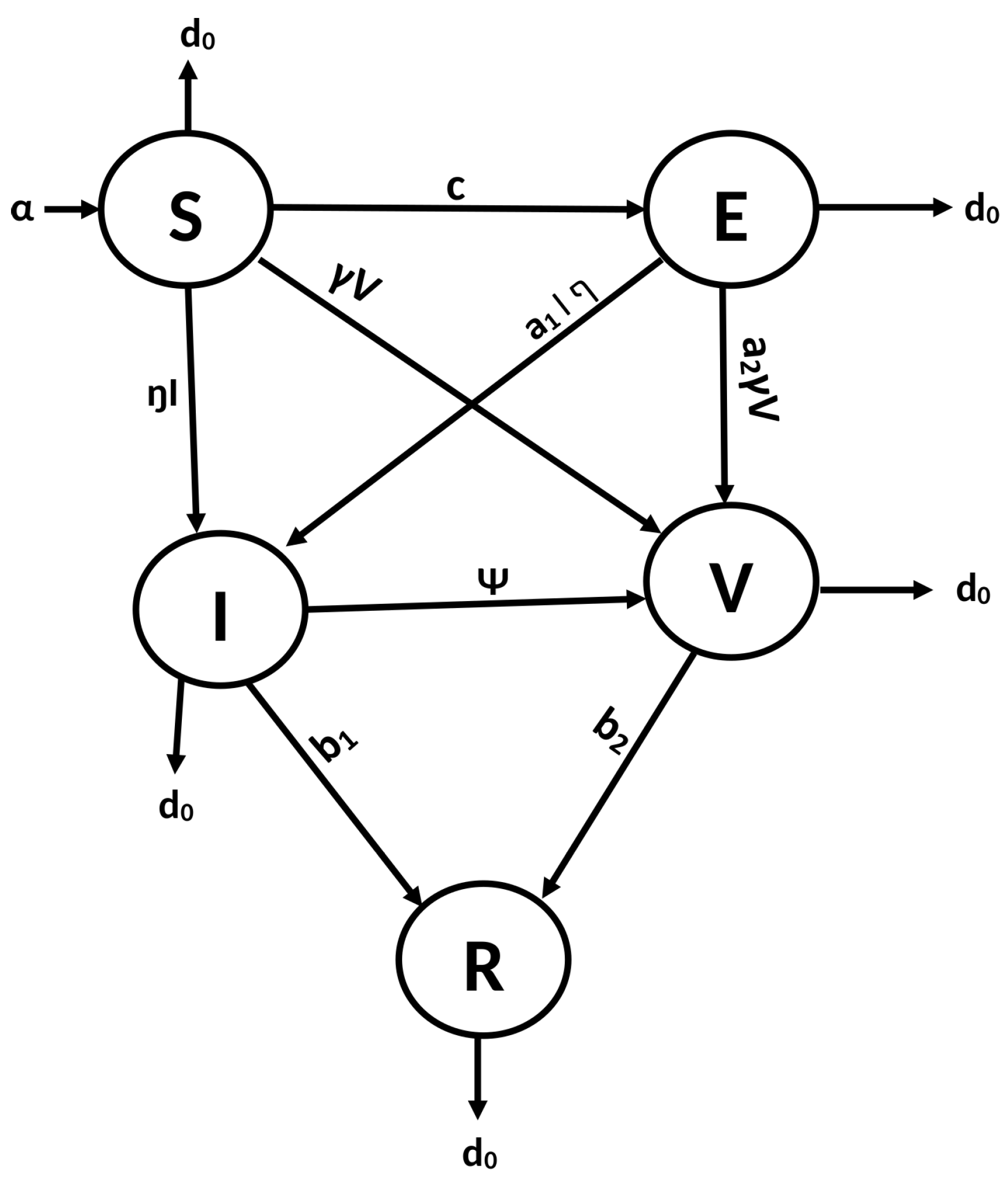
The model flowchart is shown in Figure 1.

By adding all equations of the model (1) such that the total population $\mathcal{N}=\mathcal{S}+\mathcal{E}+\mathcal{I}+\mathcal{V}+\mathcal{R}$, one has

$$\frac{d\mathcal{N}}{dt}=\alpha -d_0\mathcal{N}.$$

(2)

and hence

$$\mathcal{N}\to \frac{\alpha }{d_0}ast\to \infty .$$

Here the feasible region of the model is defined as

$$\chi =\{(\mathcal{S},\mathcal{E},\mathcal{I},\mathcal{V},\mathcal{R}):0\le \mathcal{S},\mathcal{E},\mathcal{I},\mathcal{V},\mathcal{V},\mathcal{R},\mathcal{S}+\mathcal{E}+\mathcal{I}+\mathcal{V}+\mathcal{V}+\mathcal{R}\le \frac{\alpha }{d_0}\}.$$

Therefore, we checked only the solution in feasible region $\chi$ under initial conditions, from which the uniqueness, usual existence and results can be obtained.

4. Mathematical Analysis

Here, we present some results regarding global and local stability equilibrium points computation and the calculation of ${\mathcal{R}}_0$.

4.1. Disease-Free Equilibrium Points

We analyzed whether the system is in an equilibrium (1). The model’s disease-free equilibrium (1) is represented by ${\mathcal{P}}^0=({\mathcal{S}}^0,0,0,{\mathcal{V}}^0,0)$

$$\begin{array}{cc}& {\mathcal{S}}^0=\frac{\alpha }{d_0+c}\hfill \\ & {\mathcal{V}}^0=\frac{c\alpha }{(d_0+c)d_0}\hfill \\ & {\mathcal{N}}^0=\frac{\alpha }{d_0}.\hfill \end{array}$$

4.2. Endemic Equilibrium

Also, the endemic equilibrium is computed as

$$\begin{array}{cc}& {\mathcal{S}}^{*}\left(t\right)=\frac{(d_0+\Psi +b_2)(d_0+a_1\eta \mathcal{I}+a_2\gamma \mathcal{V})}{\gamma (d_0+a_1\eta \mathcal{I}+a_2\gamma \mathcal{V}+c{a}_2)}\hfill \\ & {\mathcal{E}}^{*}\left(t\right)=\frac{c(d_0+\Psi +b_2)}{\gamma (d_0+a_1\eta \mathcal{I}+a_2\gamma \mathcal{V}+c{a}_2)}\hfill \\ & {\mathcal{V}}^{*}\left(t\right)=\left(\frac{d_0+b_1}{\Psi }-\frac{\eta (d_0+\Psi +b_2)}{\gamma \Psi }\right)\mathcal{I}\hfill \\ & {\mathcal{I}}^{*}\left(t\right)=\frac{(b_1+d_0)(d_0+a_1\eta \mathcal{I}+a_2\mathcal{V})(\eta \mathcal{I}+c+d_0+\gamma \mathcal{V})-\eta \alpha (d_0+a_1\eta \mathcal{I}+a_2\mathcal{V})-a_1\eta c\alpha }{(\eta \mathcal{I}+c+d_0+\gamma \mathcal{V})(d_0+a_1\eta \mathcal{I})+a_2\mathcal{V}}\hfill \\ & {\mathcal{R}}^{*}\left(t\right)=\frac{b_1{\mathcal{I}}^{*}+b_2{\mathcal{V}}^{*}}{d_0}.\hfill \end{array}$$

5. Expression for ${\mathcal{R}}_{\mathbf{0}}$

The basic reproduction number, or ${\mathcal{R}}_0$, is a concept used in epidemiology to describe how diseases spread and are managed. We may infer from ${\mathcal{R}}_0$ how the sickness is spreading across the population and the most effective measures to safeguard the local population against this dangerous virus. The next-generation approach is utilized to find ${\mathcal{R}}_0$ as shown below. let $\chi =(\mathcal{E},\mathcal{I})$; then, from system (1), we have

$$\frac{d\succ }{dt}=\mathcal{F}-\mathcal{V}$$

where

$$\begin{array}{c}\hfill \mathcal{F}=\left(\begin{array}{c}\eta \mathcal{S}\mathcal{I}+a_1\eta \mathcal{V}\mathcal{I}\\ \gamma \mathcal{V}\mathcal{S}+a_2\gamma \mathcal{E}\mathcal{V}\\ 0\\ 0\\ 0\end{array}\right)\end{array}$$

and

$$\mathcal{V}=\left(\begin{array}{c}(d_0+b_1)\mathcal{I}-\Psi \mathcal{V}\\ (d_0+\Psi +b_2)\mathcal{V}\\ d_0\mathcal{E}-c\mathcal{S}+a_1\eta \mathcal{I}\mathcal{E}+a_2\gamma \mathcal{E}\mathcal{V}\\ d_0\mathcal{R}-b_1\mathcal{I}-b_2\mathcal{V}\\ -\alpha +(d_0+c)\mathcal{S}+\eta \mathcal{S}\mathcal{I}+\gamma \mathcal{V}\mathcal{S}\end{array}\right)$$

The Jacobian of $\mathcal{F}$ for the disease-free equilibrium is

$$\mathcal{D}\mathcal{F}\left(Q^0\right)=\left(\begin{array}{cccc}\mathcal{F}& 0& 0& 0\\ 0& 0& 0& 0\\ 0& 0& 0& 0\\ 0& 0& 0& 0\end{array}\right),$$

and for the disease-free equilibrium, the Jacobian of $\mathcal{V}$ is given

$$\mathcal{D}\mathcal{N}\left(Q^0\right)=\left(\begin{array}{ccccc}\mathcal{N}& 0& 0& 0& 0\\ a_1\eta {\mathcal{V}}^0& a_2\gamma {\mathcal{V}}^0& d_0& 0& -c\\ -b_1& -b_2& -\beta & d_0& 0\\ \eta {\mathcal{S}}^0& \gamma {\mathcal{S}}^0& 0& 0& d_0+c\end{array}\right).$$

Hence

$$F=\left(\begin{array}{cc}\eta {\mathcal{S}}^0+a_1\eta {\mathcal{E}}^0& 0\\ 0& \gamma {\mathcal{S}}^0+a_2\gamma {\mathcal{E}}^0\end{array}\right).$$

We have

$$V=\left(\begin{array}{cc}{d}_0+b_1& -\Psi \\ 0& d_0+\Psi +b_2\end{array}\right).$$

Our constructed model behaves like [36] a double-strain model along with the infection and exposed compartments. From $F{N}^{-1}$, the above system has the following two values

$${\mathcal{R}}_1=\frac{\eta \alpha (d_0+a_{1}c)}{(d_0+b_1)(d_0+c)d_0},$$

and

$${\mathcal{R}}_2=\frac{\gamma \alpha (d_0+a_{2}c)}{(d_0+b_2+\Psi )(d_0+c)(d_0+\beta )}.$$

The productive reproduction number is the maximum value of ${\mathcal{R}}_1$ or ${\mathcal{R}}_2$ for the model (1). Given the basic reproduction number ${\mathcal{R}}_0$, we established the following result.

Theorem 1.

(i) There does not exist a positive equilibrium ${\mathcal{E}}^0$ for the model (1) if ${\mathcal{R}}_1<1$ and/or ${\mathcal{R}}_2<1$.

(ii) There exists a distinct positive (unique) equilibrium ${\mathcal{E}}^{*}=({\mathcal{S}}^{*},{\mathcal{E}}^{*},{\mathcal{I}}^{*},{\mathcal{V}}^{*},{\mathcal{R}}^{*})$, which is also called an endemic equilibrium, if ${\mathcal{R}}_1\le 1$ and/or ${\mathcal{R}}_2\le 1$.

Proof. 

(i) The Jacobian matrix at ${\mathbb{E}}^0$ is given below

${\mathcal{M}}^0=\left[\begin{array}{ccccc}-(d_0+b_1)+\eta \left({\mathcal{S}}^0\right)& \Psi & 0& 0& 0\\ 0& -(d_0+\Psi +b_2)+\gamma ({\mathcal{S}}^0+a_2\mathcal{E})& 0& 0& 0\\ -a_1\eta {\mathcal{E}}^0& -a_2\gamma {\mathcal{E}}^0& -d_0& 0& 0\\ b_1& b_2& 0& -d_0& 0\\ -\eta {\mathcal{S}}^0& -\gamma {\mathcal{S}}^0& 0& 0& -(d_0+c)\end{array}\right],$

and

$$|\lambda -{\mathcal{M}}^0\left(\mathcal{Q}\right)|=0.$$

Hence

$$\begin{array}{cc}& {\lambda }_1=-d_0\hfill \\ & {\lambda }_2=-d_0\hfill \\ & {\lambda }_3=-(d_0+c)\hfill \\ & {\lambda }_4=(d_0+b_1)({\mathcal{R}}_1-1)\hfill \\ & {\lambda }_5=-(d_0+\Psi +b_2)+\gamma ({\mathcal{S}}^0+a_2{\mathcal{E}}^0)=(d_0+\Psi +b_2)({\mathcal{R}}_2-1).\hfill \end{array}$$

${\lambda }_1$, ${\lambda }_2$ and ${\lambda }_3$ are strictly negative. The signs of ${\lambda }_4$ and ${\lambda }_5$ depend on $({\mathcal{R}}_1-1)$ and $({\mathcal{R}}_2-1)$, which follow the conclusion.

(ii) See Theorem 3. □

6. Mathematical Stability Analysis

This section examines the equilibrium point’s characteristics along with the system’s local and overall stability (1). Additionally, the system’s overall analysis and the equilibrium’s characteristics are outlined (1).

6.1. Local Stability

In this part of our work, we discuss the local stability of the system (1). By using the Jacobian matrix, the next theorem is presented to obtain the required results.

Theorem 2.

If ${\mathcal{R}}_1<1$ and/or ${\mathcal{R}}_2<1$, the disease-free equilibrium ${\mathcal{E}}^0$ is locally asymptotically stable, and vice versa.

Proof. 

The Jacobian matrix at ${\mathbb{E}}^0$ is given below

${\mathcal{M}}^0=\left[\begin{array}{ccccc}-(d_0+b_1)+\eta \left({\mathcal{S}}^0\right)& \Psi & 0& 0& 0\\ 0& -(d_0+\Psi +b_2)+\gamma ({\mathcal{S}}^0+a_2\mathcal{E})& 0& 0& 0\\ -a_1\eta {\mathcal{E}}^0& -a_2\gamma {\mathcal{E}}^0& -d_0& 0& 0\\ b_1& b_2& 0& -d_0& 0\\ -\eta {\mathcal{S}}^0& -\gamma {\mathcal{S}}^0& 0& 0& -(d_0+c)\end{array}\right],$

and

$$|\lambda -{\mathcal{M}}^0\left(\mathcal{Q}\right)|=0.$$

Hence

$$\begin{array}{cc}& {\lambda }_1=-d_0\hfill \\ & {\lambda }_2=-d_0\hfill \\ & {\lambda }_3=-(d_0+c)\hfill \\ & {\lambda }_4=-(d_0+b_1)({\mathcal{R}}_1-1)\hfill \\ & {\lambda }_5=-(d_0+\Psi +b_2)+\gamma ({\mathcal{S}}^0+a_2{\mathcal{E}}^0)=(d_0+\Psi +b_2)({\mathcal{R}}_2-1).\hfill \end{array}$$

${\lambda }_1$, ${\lambda }_2$ and ${\lambda }_3$ are strictly negative. The signs of ${\lambda }_4$ and ${\lambda }_5$ depend on $({\mathcal{R}}_1-1)$ and $({\mathcal{R}}_2-1)$. Disease-free stability shows the dynamical behavior of an individual population whenever a very small emergent proportion of the infected migrate. Note that if ${\mathcal{R}}_1<1$ and ${\mathcal{R}}_2<1$, then ${\lambda }_4$ and ${\lambda }_5$ are strictly negative. Hence, the system is asymptotically stable locally.

Given the existence of an endemic equilibrium, we take the positive solution of

$$P\left(I\right)=k_1{\mathcal{I}}^2+k_2\mathcal{I}+k_3=0,$$

where

$$\begin{array}{cc}& k_1=\left(a_1\eta +a_2\gamma \left(\frac{d_0+b_1}{\Psi }-\frac{(d_0+\Psi +b_2)}{\gamma \Psi }\right)\right)\left(\gamma \left(\frac{d_0+b_1}{\Psi }-\frac{(d_0+\Psi +b_2)}{\gamma \Psi }\right)\right)\hfill \\ & k_2=[(d_0+\eta )\left(\gamma \left(\frac{d_0+b_1}{\Psi }-\frac{(d_0+\Psi +b_2)}{\gamma \Psi }\right)\right)+(d_0+c)\left(a_1\eta +a_2\gamma \left(\frac{d_0+b_1}{\Psi }-\frac{\eta (d_0+\Psi +b_2)}{\gamma \Psi }\right)\right)\hfill \\ & -\alpha \gamma \frac{a_1\eta +a_2\gamma (\frac{d_0+b_1}{\Psi }-\frac{\eta (d_0+\Psi +b_2)}{\gamma \Psi })}{d_0+\Psi +b_2}]\hfill \\ & k_3=(d_0+\eta )(d_0+c)-\alpha \gamma \frac{d_0{a}_{2}c}{d_0+\Psi +b_2}\hfill \\ & or\hfill \\ & k_3=(d_0+\beta )(d_0+c)(1-{\mathcal{R}}_2).\hfill \end{array}$$

(3)

□

6.2. Global Stability

Global stability is investigated through a function called the Lyapnuov function. We constructed a Lyapnuov function to investigate the global stability of the model (1).

Theorem 3.

If ${\mathcal{R}}_1\le 1$ and/or ${\mathcal{R}}_2\le 1$, then the endemic equilibrium ${\mathcal{E}}^{*}$ of the model (1) is globally stable in χ.

Proof. 

To prove this theorem result, we constructed a function called a Lyapnuov function.

$$\mathcal{W}=C_1(\mathcal{S}-{\mathcal{S}}^0)+C_2(\mathcal{E}-{\mathcal{E}}^0)+C_3(\mathcal{V}-{\mathcal{V}}^0)+C_4\mathcal{I}.$$

(4)

Here, $C_1$, $C_2$, $C_3$ and $C_4$ are constants. Now, w.r.t t takes the derivative of the above equation.

$$\dot{\mathcal{W}}=C_1\dot{\mathcal{S}}+C_2\dot{\mathcal{E}}+C_3\dot{\mathcal{V}}+C_4\mathcal{I}.$$

After, some basic calculation

$$\begin{array}{cc}& \dot{W}=C_1\left[\alpha -\eta \mathcal{S}\mathcal{I}-(c+d_0)\mathcal{S}-\gamma \mathcal{V}\mathcal{S}\right]+C_2\left[c\mathcal{S}-(\beta +d_0)\mathcal{E}-a_1\eta \mathcal{I}\mathcal{E}-a_2\gamma \mathcal{V}\mathcal{E}\right]\hfill \\ & +C_3\left[\eta \mathcal{S}\mathcal{I}+a_1\eta \mathcal{I}\mathcal{E}+\Psi \mathcal{V}-(b_1+d_0)\mathcal{I}\right]\hfill \\ & +C_4\left[\gamma \mathcal{V}\mathcal{S}-(\Psi +d_0+b_2)\mathcal{V}+a_2\gamma \mathcal{V}\mathcal{E}\right].\hfill \end{array}$$

$$\begin{array}{ccc}\hfill \dot{W}& =& \eta \mathcal{S}\mathcal{I}(C_3-C_1)+c(C_2-C_1)+\gamma \mathcal{V}\mathcal{S}(C_3-C_1)+a_1\eta \mathcal{I}\mathcal{E}(C_3-C_1)\hfill \\ & +& a_2\gamma \mathcal{E}\mathcal{V}(C_4-C_2)+\Psi \mathcal{V}(C_3+C_1)-C_2\beta \mathcal{E}-C_2{d}_0\mathcal{E}\hfill \\ & -& C_3{b}_1\mathcal{I}-C_3{d}_0\mathcal{I}-C_4{d}_0\mathcal{V}-C_4{d}_0\mathcal{V}-C_4{b}_2\mathcal{V}.\hfill \end{array}$$

Let $C_1=C_2=C_3=1$; we obtain

$$\dot{W}=-(C_2\beta \mathcal{E}+C_2{d}_0\mathcal{E}+C_3{b}_1\mathcal{I}+C_3{d}_0\mathcal{I}+C_4{d}_0\mathcal{V}+C_4{d}_0\mathcal{V}+C_4{b}_2\mathcal{V})<0.$$

If ${\mathcal{R}}_1$ and/or ${\mathcal{R}}_2>1$, the system is globally asymptotically stable. □

7. Numerical Results and Discussion

In this section of our paper, we will discuss the results of a vaccine study conducted in Pakistan. The currently running simulation offers information and outcomes that are of a general nature and can be generalized to any kind of place. It is divided into the following five sections: susceptible, exposed, infected, vaccinated and recovered. Lockdown, quarantine and evacuation from affected areas are some of the major measures that can be taken to combat the disease. It is estimated that there are 3.9 deaths for every thousand people living in Saudi Arabia, while there are 14.56 births for every thousand people. The vaccination program began in the middle of Saudi Arabia in December 2020 with the aim of reaching 65 percent of the adult population by November 2021. The vaccination rate in 2021 was 0.00127. We sought to investigate whether this would be sufficient to completely eradicate the disease.

Here, the nonstandard finite difference scheme was used [12,26] to rewrite the system in differential equation form as for first equation of system (1) as

$$\frac{d\mathcal{S}\left(t\right)}{dt}=\alpha -\eta \mathcal{S}\mathcal{I}+(c+d_0)\mathcal{S}-\gamma \mathcal{S}\mathcal{V}.$$

(5)

Which is decomposed in the proposed scheme as

$$\begin{array}{c}\hfill \frac{{\mathcal{S}}_{j+1}-{\mathcal{S}}_j}{h}=\alpha -\eta {\mathcal{S}}_j{\mathcal{I}}_j+(c+d_0){\mathcal{S}}_j-\gamma {\mathcal{S}}_j{\mathcal{V}}_j.\end{array}$$

(6)

Like (6), using the nonstandard finite difference scheme, we decomposed the system (1) as follows

$$\begin{array}{ccc}\hfill {\mathcal{S}}_{j+1}& =& {\mathcal{S}}_{j+h}\left(\alpha -\eta {\mathcal{S}}_j{\mathcal{I}}_j+(c+d_0){\mathcal{S}}_j-\gamma {\mathcal{S}}_j{\mathcal{V}}_j\right)\hfill \\ \hfill {\mathcal{E}}_{j+1}& =& {\mathcal{E}}_{j+h}\left(c{\mathcal{S}}_j-d_0{\mathcal{E}}_j-a_1\eta {\mathcal{I}}_j{\mathcal{E}}_j-a_2\gamma {\mathcal{V}}_j{\mathcal{E}}_j\right)\hfill \\ \hfill {\mathcal{I}}_{j+1}& =& {\mathcal{I}}_{j+h}\left(\eta {\mathcal{S}}_j{\mathcal{I}}_j+a_1\eta {\mathcal{I}}_j{\mathcal{E}}_j+\Psi {\mathcal{V}}_j-(b_1+d_0){\mathcal{I}}_j\right)\hfill \\ \hfill {\mathcal{V}}_{j+1}& =& {\mathcal{V}}_{j+h}\left(\gamma {\mathcal{S}}_j{\mathcal{V}}_j-(\Psi +d_0+b_2){\mathcal{V}}_{\mathcal{j}}+a_2\gamma {\mathcal{V}}_j{\mathcal{E}}_j\right)\hfill \\ \hfill {\mathcal{R}}_{j+1}& =& {\mathcal{R}}_{j+h}\left(b_1{\mathcal{I}}_j+b_2{\mathcal{V}}_j-d_0{\mathcal{R}}_j\right).\hfill \end{array}$$

(7)

We use nonstandard finite difference scheme (7) for graphical presentation of our model (1) by using

Table 2. Description and specification of the system’s parameters approximate real values (1).

Parameter	Physical Description	Approximate Value
$\mathcal{S}$	Susceptible class	$217.342565$ in millions [37]
$\mathcal{E}$	Exposed class	100 in million (assumed)
$\mathcal{I}$	Infected class	$1.386348$ in million [37]
$\mathcal{V}$	Vaccination class	$0.271087$ in million [37]
$\mathcal{R}$	Recovered class	$1.271087$ in million [37]
$\alpha$	Immigrant to susceptible compartment	1.35 (assumed)
$d_0$	Natural death	0.000065 [37]
$\beta$	Recovery rate from exposed	1.43 (assumed)
c	Exposed rate	0.00019 (assumed)
$a_1$	Infection constant	0.0008601 (assumed)
$a_2$	Vaccination constant	0.0008601 (assumed)
$b_1$	Recovery from infection compartment	0.10 (assumed)
$b_2$	Recovery from vaccination	0.98 (assumed)
$\eta$	Infection rate	0.020 (assumed)
$\Psi$	Loss of immunity	0.020 (assumed)
$\gamma$	Vaccination rate	0.020 (assumed)

. To understand the dynamics of the system, we used real data of Saudi Arabia for the simulation.

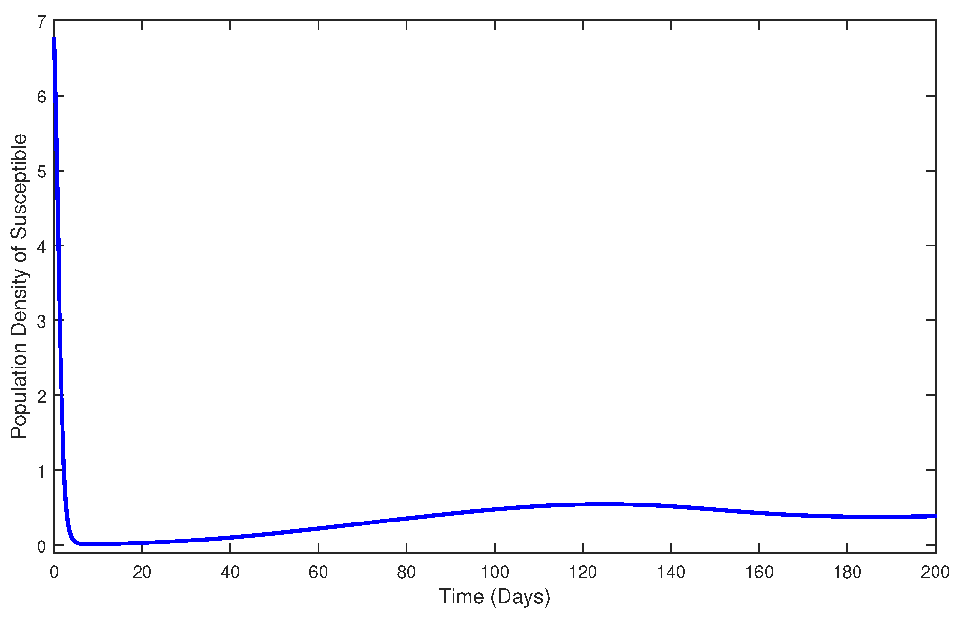
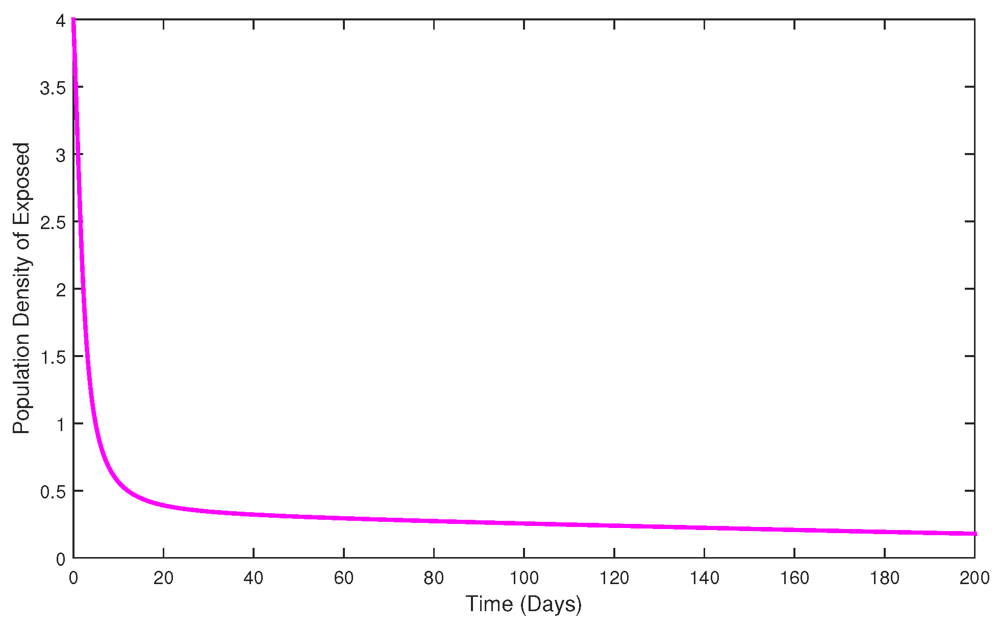
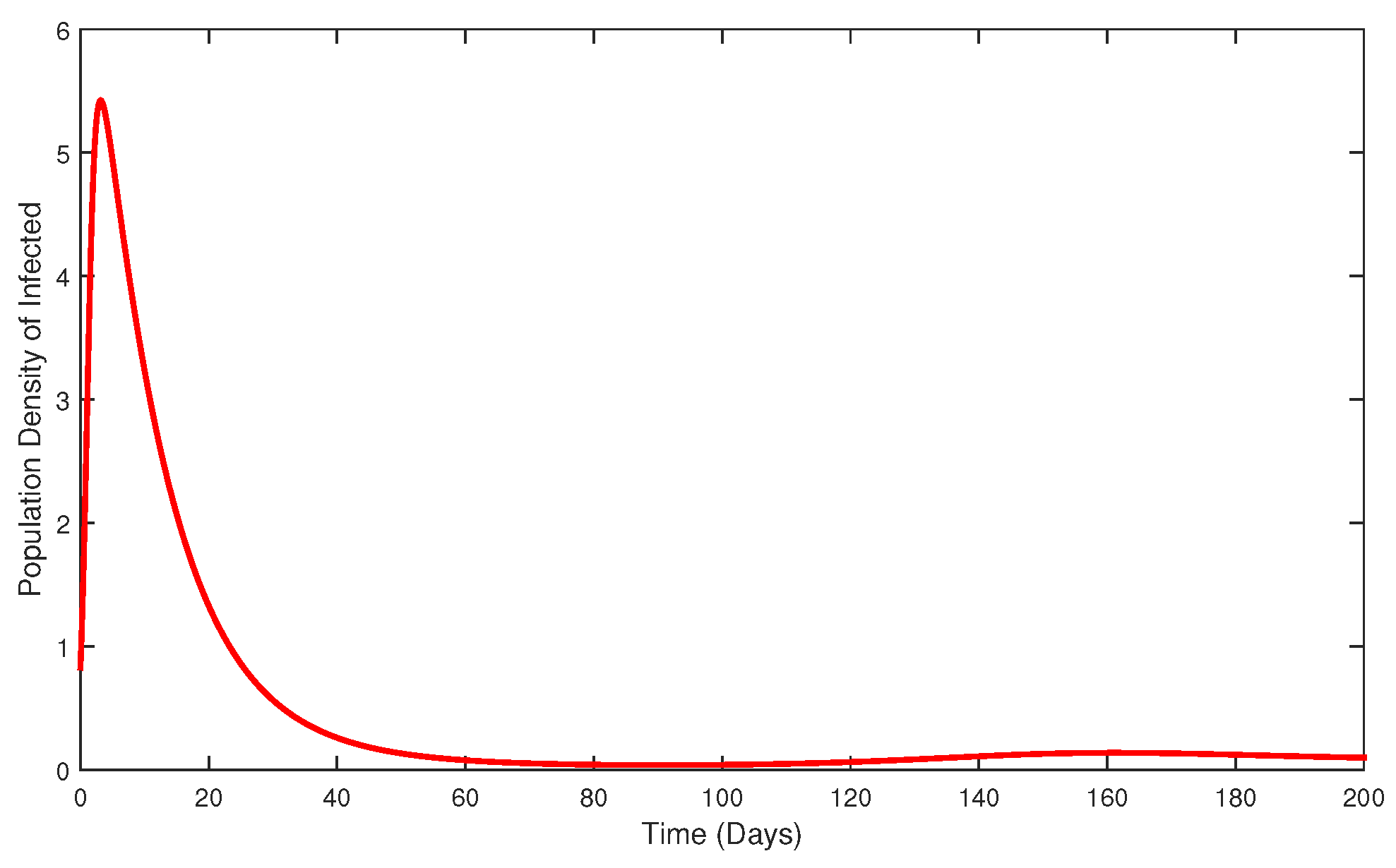
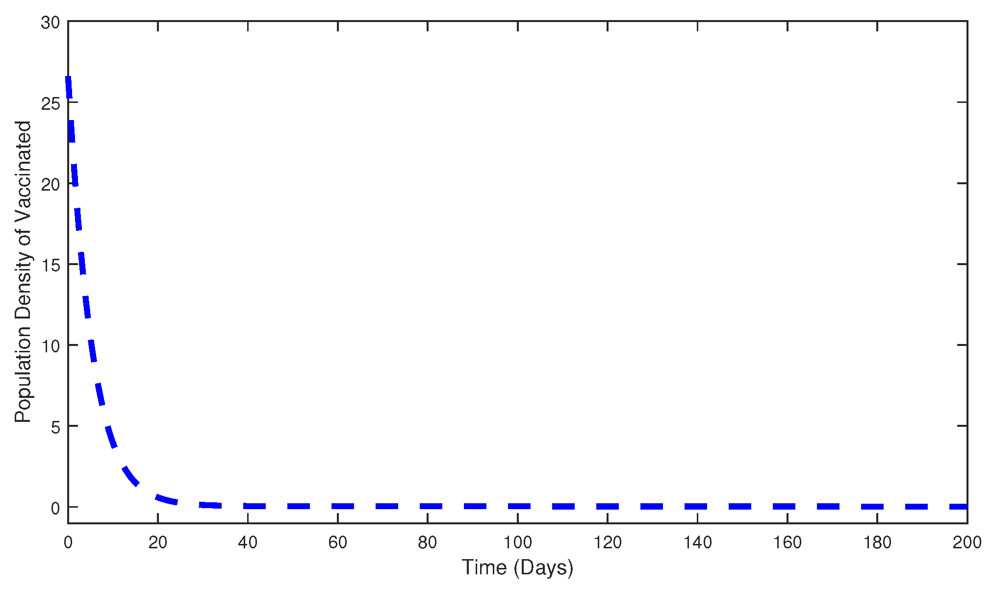
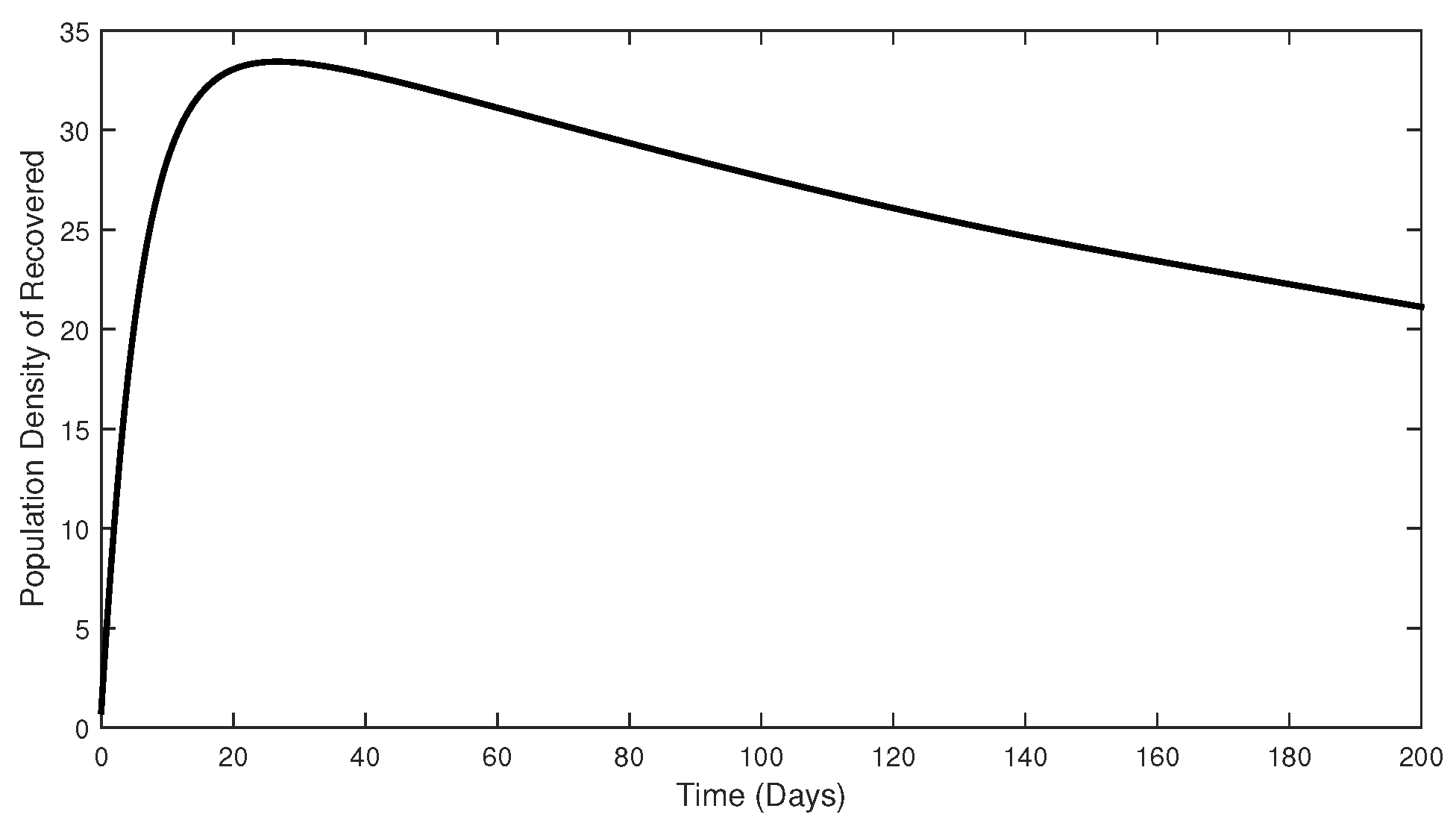
We provide the dynamical behaviors of different classes of the suggested model in Figure 2, Figure 3, Figure 4, Figure 5 and Figure 6 for a period of two hundred days by utilizing the reference Table 2. These behaviors reveal that there is a decrease in the sensitive and exposed compartments, while there is an increase in the infection class. However, vaccination causes the infection class to decline, which results in an increase in the recovered class. Therefore, vaccination brings a reduction in the prevalence of disease and helps maintain its status. This demonstrates that our current model is a valid one.

8. Numerical Treatment via Fractional Calculus

We investigated our model in the form of fractional calculus. For this purpose, we used the Caputo-type fractional derivative and Riemann–Liouville-type integral defined as below:

Definition 1

([27]). Integral of non-integer order $\beta >0$ of a function $\mathcal{S}:[0,\infty )\to \mathbb{R}$ is defined as

$$I_t^{\phi }\mathcal{S}\left(t\right)=\frac{1}{\chi \left(\alpha \right)}{\int }_0^t\frac{\mathcal{S}\left(\eta \right)}{{(t-\eta )}^{1-\alpha }}d\eta ,$$

provided the integral exists at the right sides.

Moreover, by definition of Caputo, we have

$$D_{0+}^{\alpha }\mathcal{S}\left(t\right)=\left\{\begin{array}{cc}\hfill & \frac{1}{\chi (1-\alpha )}{\int }_0^t{(t-\eta )}^{-\alpha }{\mathcal{S}}^{{}^{\prime }}\left(\eta \right)d\eta ,0<\alpha \le 1,\hfill \\ & \frac{d\mathcal{S}}{dt},\alpha =1.\hfill \end{array}\right.$$

For fractional order

$$\begin{array}{ccc}\hfill {\mathcal{D}}_t^{\alpha }& =& F(t,X),\hfill \\ \hfill X\left(0\right)& =& X_0\hfill \end{array}$$

(8)

where

$$X=(\mathcal{S},\mathcal{E},\mathcal{I},\mathcal{V},\mathcal{R}),X_0=({\mathcal{S}}_0,{\mathcal{E}}_0,\mathcal{I},{\mathcal{V}}_0,{\mathcal{R}}_0).$$

Then, the generalized form of the Taylor series is used, as follows

$$\begin{array}{c}\hfill X(t+h)=X\left(t\right)+\frac{h^{\alpha }}{\chi (\alpha +1)}{\mathcal{D}}_t^{\alpha }X\left(t\right)+\frac{h^{2\alpha }}{\chi (2\alpha +1)}{\mathcal{D}}_t^{2\alpha }X\left(t\right)+\dots \end{array}$$

(9)

By using fractional calculus results, we have ${\mathcal{D}}_t^{2\alpha }X={\mathcal{D}}_t^{\alpha }E(t,Y)+E(t,Y){\mathcal{D}}_Y^{\alpha }E(t,Y).$ Using (9), we obtained the general form after some rearranging of terms as follows,

$$Y(t+h)=Y\left(t\right)+\frac{h^{\alpha }}{\chi (\alpha +1)}E(t,Y\left(t\right))+\frac{h^{\alpha }}{2\chi (\alpha +1)}\left[{\mathbf{K}}_1+{\mathbf{K}}_2\right],$$

(10)

where

$${\mathbf{K}}_1=E(t_j,Y_j\left(t_j\right)),{\mathbf{K}}_2=E\left(t_j+\frac{2h^{\alpha }\chi (\alpha +1)}{\chi (2\alpha +1)},Y\left(t_j\right)+\frac{2h^{\alpha }\chi (\alpha +1)}{\chi (2\alpha +1)}E(t_j,Y_j\left(t_j\right))\right).$$

Let assume $\alpha =1$; then, we obtain the classical required scheme (6) by using the Caputo fractional derivative order for different fractional order Figure 3.

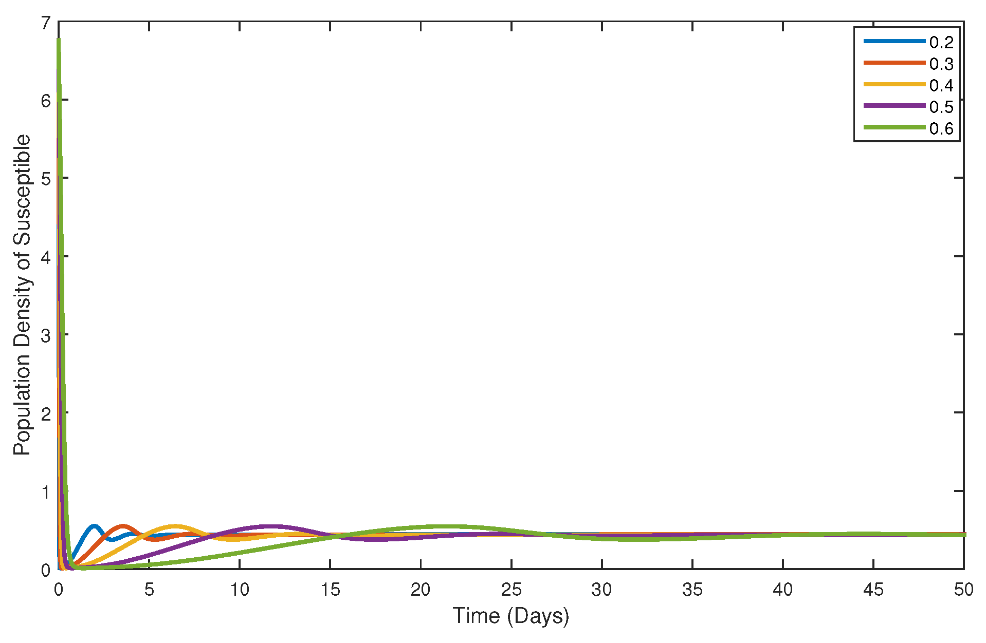
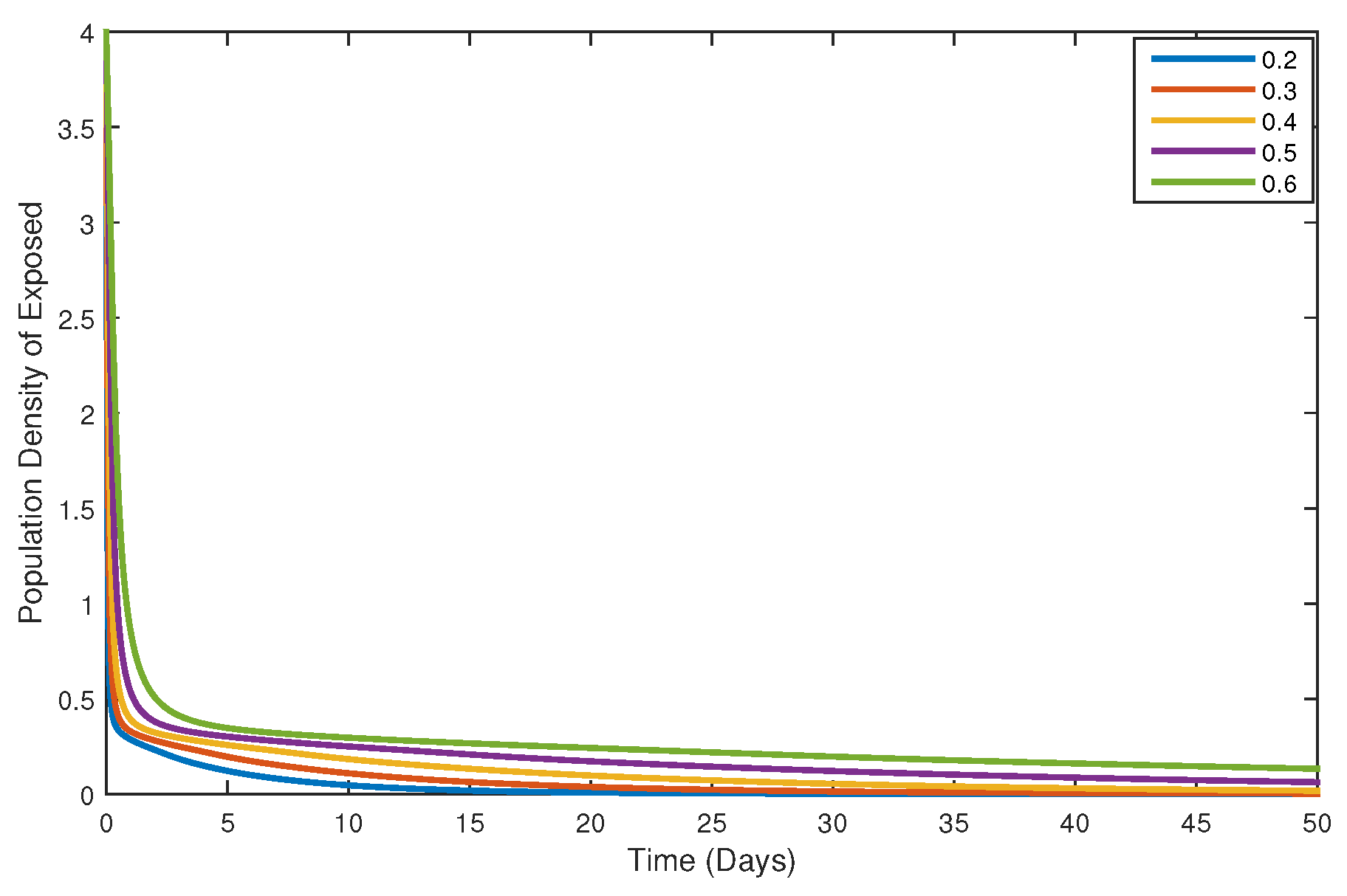
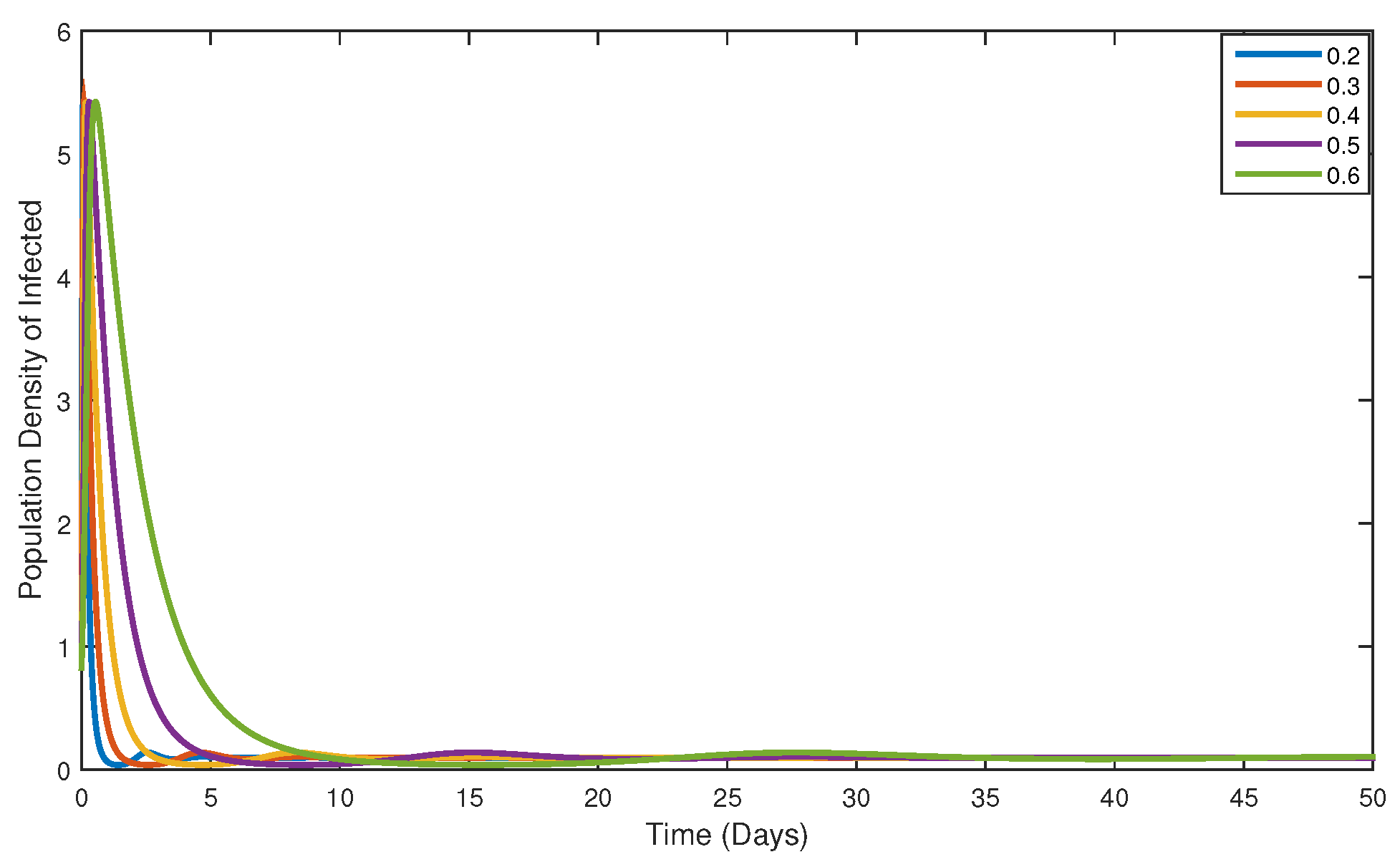
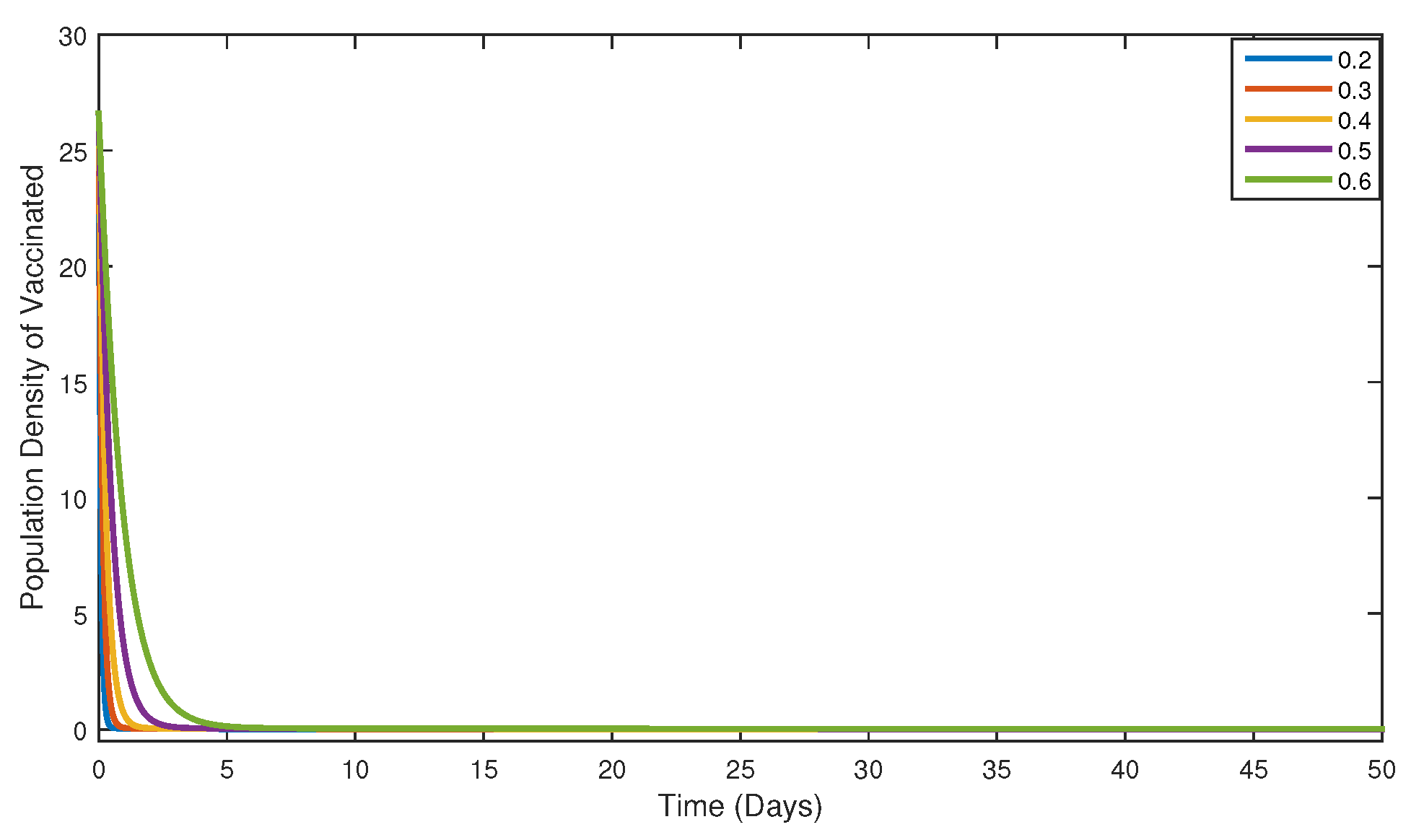
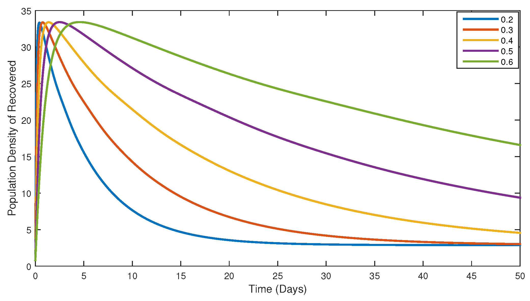
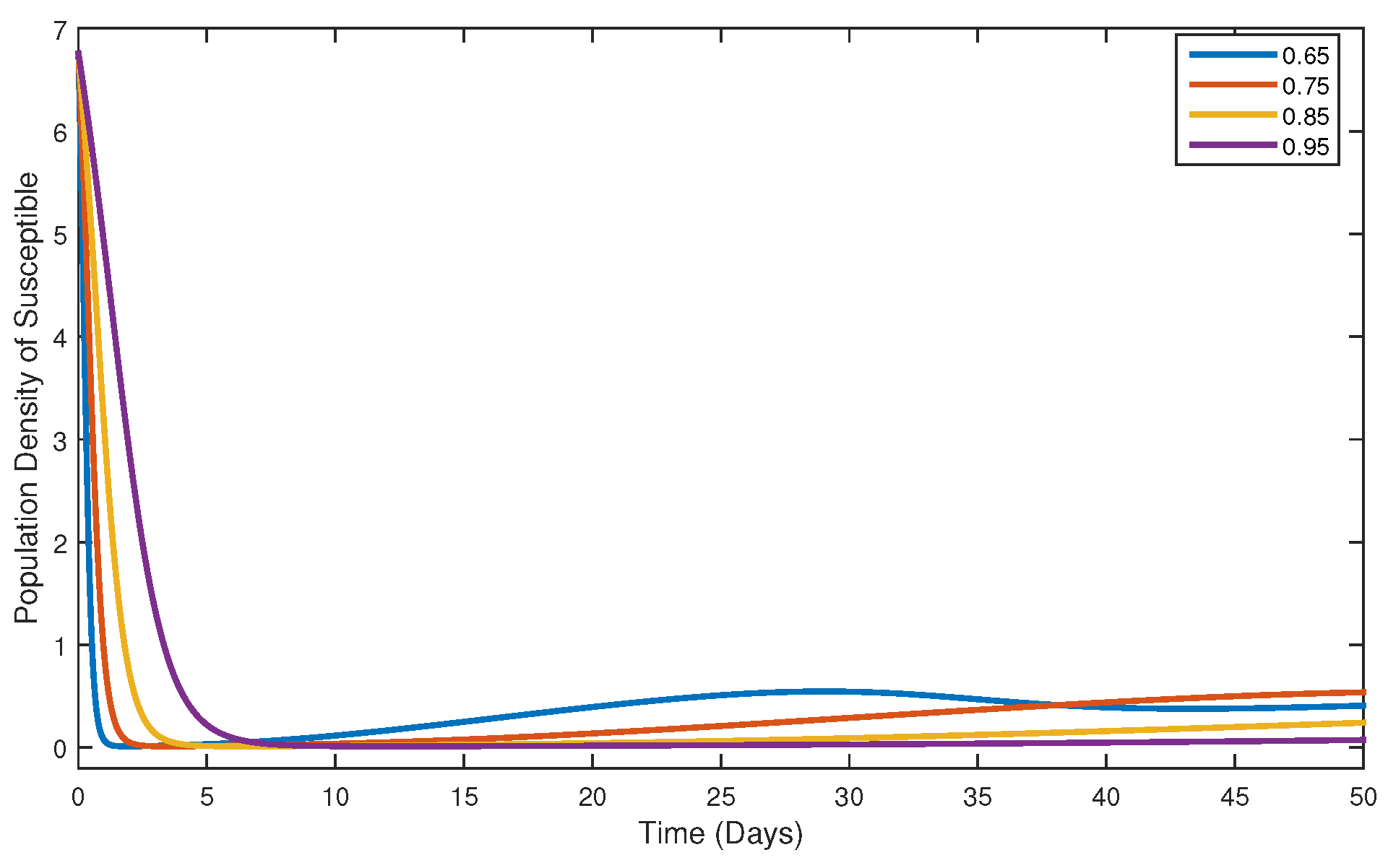
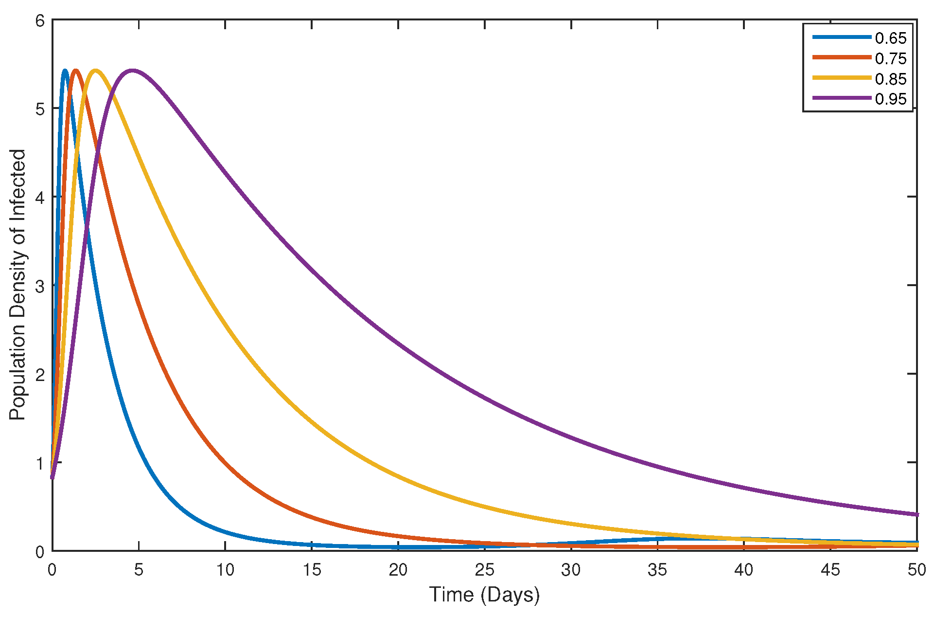
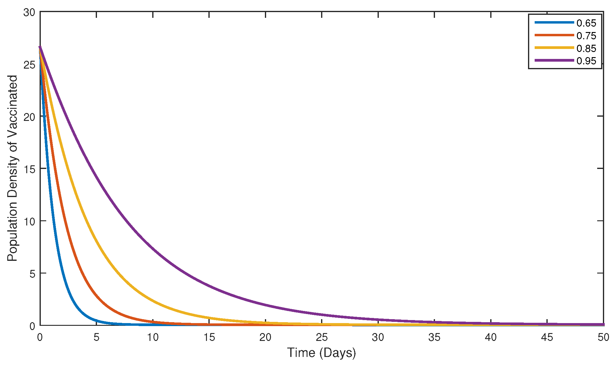
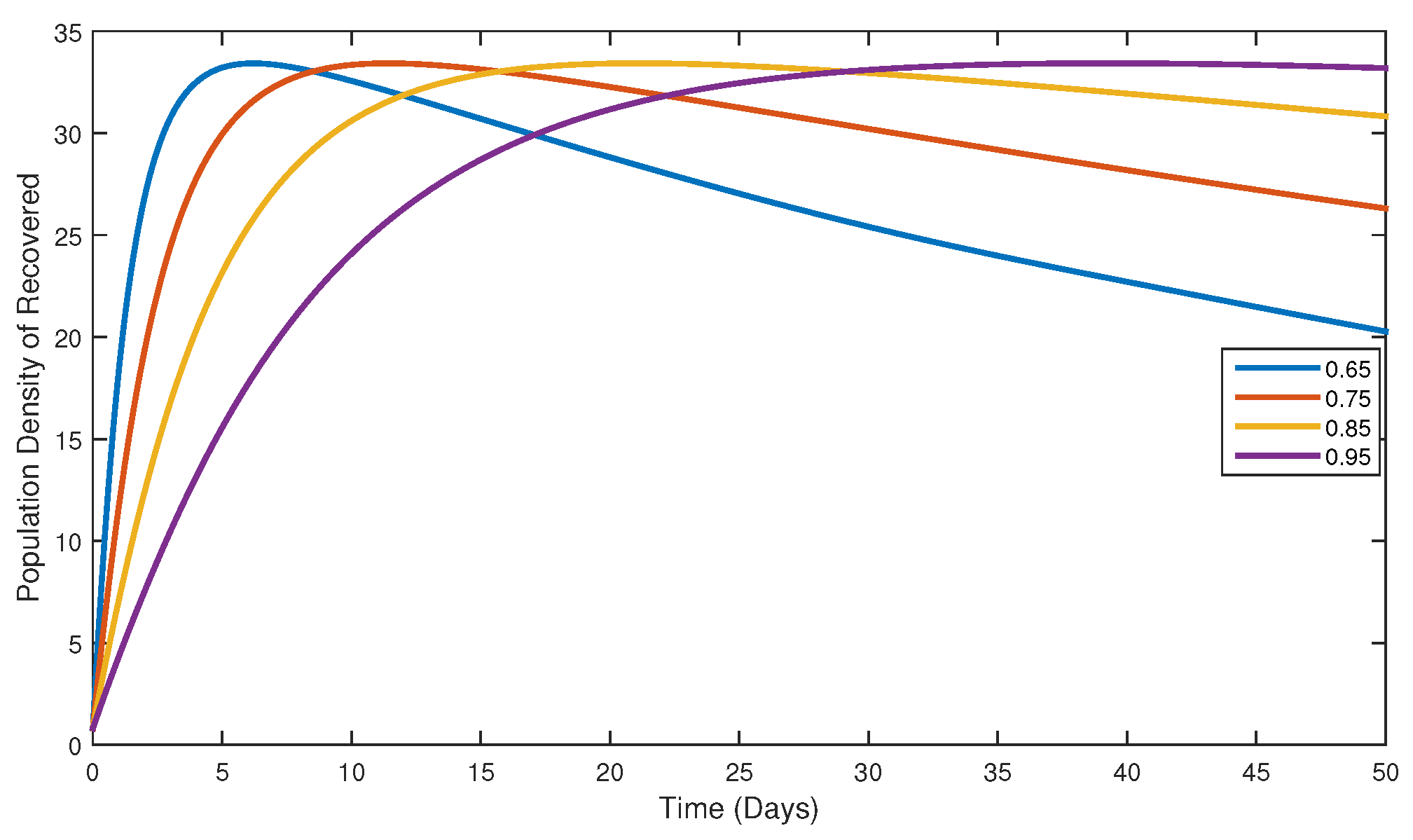
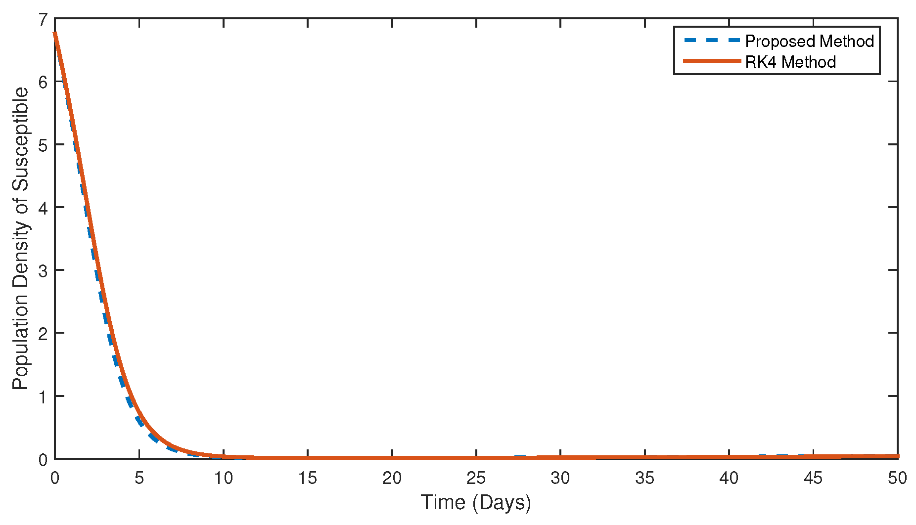
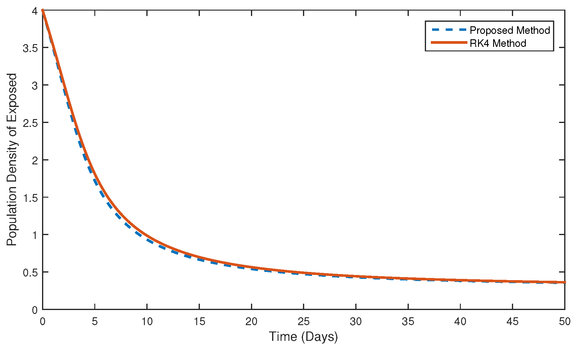
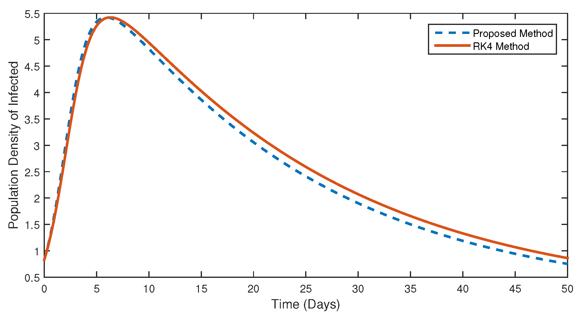
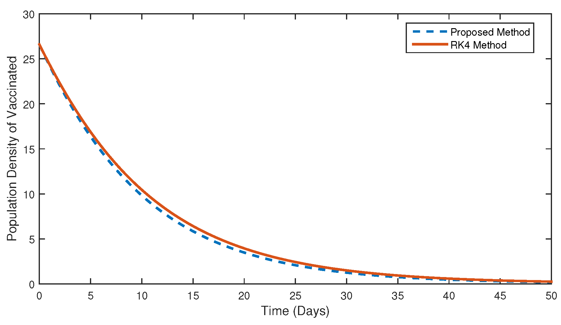
The numerical findings of the various compartments are shown for a variety of fractional orders in the figures referenced from Figure 7, Figure 8, Figure 9, Figure 10, Figure 11, Figure 12, Figure 13, Figure 14, Figure 15 and Figure 16. When compared to the dynamical behaviors of distinct classes at greater fractional order values, we observe that these behaviors change when the fractional order is reduced to a smaller number. In the same manner, in order to validate the validity of the numerical scheme for the fractional order, we compared the numerical outcomes of the given fractional order with the well-established RK4 approach in Figure 17, Figure 18, Figure 19, Figure 20 and Figure 21 for the various compartments. This was performed in order to check the authenticity of the numerical scheme. We can see that the answer suggested by the proposed method and the one produced by RK4 have a lot in common with one another. In addition, the amount of time spent by the CPU for each approach was measured and compared using an HP Cori-5 computer of the seventh generation. From the

Table 3. Comparison between CPU time for proposed method with the RK4 method at fractional order $\alpha =0.99$.

Range of t	CPU Time of RK4 Method in Seconds	CPU Time of Nonstandard Finite Difference Scheme in Seconds
50	5.00	4.50
100	6.8	5.55
150	8.70	6.82
200	12.67	10.67
250	20.99	18.69
300	26.77	20.60

, we can observe that the proposed solution has a lower compilation time.

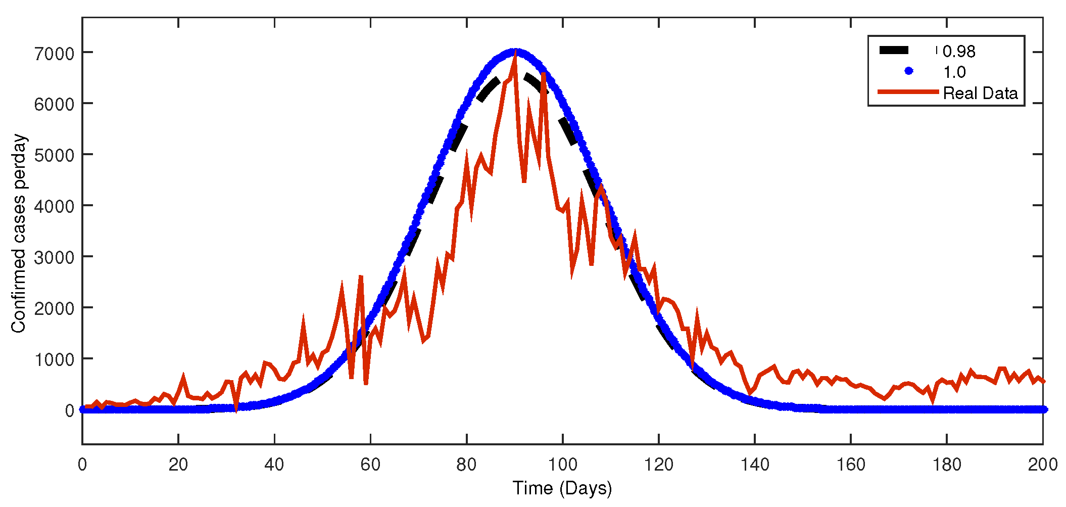
In addition, we compared the reported confirmed infected cases for 200 days in Pakistan [38] with the simulated result for the infected cases using the classical as well as fractional orders in Figure 22. This was performed in order to determine whether or not there was a correlation between the two sets of data. We can observe that the results of the fractional order are much closer to the results of the real data than the results of the integer order.

9. Conclusions

The behavior of the virus serves as the foundation for the mathematical SEIVR model for novel COVID-19 that we developed in this paper. Our primary focus is on developing a method to estimate the reaction of the population after vaccination. In the absence of a visible illness or symptoms, the major factor that differentiates this virus from other infectious diseases that may present themselves similarly is a loss of immunity to the disease. In order to provide support for this claim, an analytical equation for ${\mathcal{R}}_{\infty }$ and/or ${\mathcal{R}}_{\in }$ is utilized. This expression is a crucial component in the process of identifying the necessary and sufficient conditions for disease-free and endemic equilibrium. As proof for the conclusions we have drawn based on theory, we present actual statistics for Saudi Arabia.

The key findings and results are as follows:

We give a mathematical demonstration that shows how vaccination helps minimize the rate of disease transmission, which is an important factor in the overall fight against the illness. We use mathematics to illustrate that the vaccination effort in Saudi Arabia was a response to the increased number of diseases that were occurring in that country. On the basis of the data obtained from the model’s parameter values, we provide evidence to show that the rate of vaccination for COVID-19 influences the spread of the disease. According to specialists working in relevant fields, this virus has recently exhibited a variety of behavioral shifts in relatively recent times. We outline how the virus can occasionally acts differently, as expected. We are working on developing a new model in an effort to provide an explanation for the patterns that have only lately been discovered, such as Beta and Omicron. In addition to this, we contrasted our findings with those obtained by the RK4 approach. We made the observation that the numerical strategy that was proposed uses less CPU time than the RK4 technique that was mentioned. The numerical findings that were provided by our studied numerical scheme have a close relationship with those of the RK4 approach.

References

- Gumel, A.B.; Ruan, S.; Day, T.; Watmough, J.; Brauer, F.; Van den Driessche, P.; Gabrielson, D.; Bowman, C.; Alexander, M.E.; Ardal, S.; et al. Modelling strategies for controlling SARS out breaks. Proc. R. Soc. Lond. B 2004, 271, 2223–2232. [Google Scholar] [CrossRef] [PubMed]
- Sasmita, N.R.; Ikhwan, M.; Suyanto, S.; Chongsuvivatwong, V. Optimal control on a mathematical model to pattern the progression of coronavirus disease 2019 (COVID-19) in Indonesia. Glob. Health Res. Policy 2020, 5, 38. [Google Scholar] [CrossRef] [PubMed]
- Lewandowski, R.; Pawlak, Z. Dynamic analysis of frames with viscoelastic dampers modelled by rheological models with fractional derivatives. J. Sound Vib. 2011, 330, 923–936. [Google Scholar] [CrossRef]
- Atangana, E.; Atangana, A. Facemasks simple but powerful weapons to protect against COVID-19 spread: Can they have sides effects? Results Phys. 2020, 19, 103425. [Google Scholar] [CrossRef]
- Goel, N.S.; Maitra, S.C.; Montroll, E.W. On the Volterra and other nonlinear models of interacting populations. Rev. Mod. Phys. 1971, 43, 231. [Google Scholar] [CrossRef]
- Li, Q.; Guan, X.; Wu, P.; Wang, X.; Zhou, L.; Tong, Y.; Ren, R.; Leung, K.S.M.; Lau, E.H.Y.; Wong, J.Y.; et al. Early transmission dynamics in Wuhan, China, of novel coronavirus infected pneumonia. N. Engl. J. Med. 2020, 382, 1199–1207. [Google Scholar] [CrossRef]
- Bogoch, I.I.; Watts, A.; Thomas-Bachli, A.; Huber, C.; Kraemer, M.U.; Khan, K. Pneumonia of unknown aetiology in Wuhan, China: Potential for international spread via commercial air travel. J. Travel Med. 2020, 27, taaa008. [Google Scholar] [CrossRef]
- World Health Organization (WHO). Naming the coronavirus disease (COVID-19) and the virus that causes it. Braz. J. Implantol. Health Sci. 2020, 2, 4. [Google Scholar]
- Nesteruk, I. Statistics based predictions of coronavirus 2019-nCoV spreading in mainland China. medRxiv 2020. [Google Scholar] [CrossRef]
- Shah, K.; Din, R.U.; Deebani, W.; Kumam, P.; Shah, Z. On nonlinear classical and fractional order dynamical system addressing COVID-19. Results Phys. 2021, 24, 104069. [Google Scholar] [CrossRef]
- Lotka, A.J. Contribution to the theory of periodic reactions. J. Phys. Chem. 2002, 14, 271–274. [Google Scholar] [CrossRef] [Green Version]
- Khalsaraei, M.M. An improvement on the positivity results for 2-stage explicit Runge-Kutta methods. J. Comput. Appl. Math. 2010, 235, 137–143. [Google Scholar] [CrossRef] [Green Version]
- Watson, O.J.; Barnsley, G.; Toor, J.; Hogan, A.B.; Winskill, P.; Ghani, A.C. Global impact of the first year of COVID-19 vaccination: A mathematical modelling study. Lancet Infect. Dis. 2022, 22, 1293–1302. [Google Scholar] [CrossRef] [PubMed]
- Moore, S.; Hill, E.M.; Tildesley, M.J.; Dyson, L.; Keeling, M.J. Vaccination and non-pharmaceutical interventions for COVID-19: A mathematical modelling study. Lancet Infect. Dis. 2021, 21, 793–802. [Google Scholar] [CrossRef] [PubMed]
- Yavuz, M.; Coşar, F.O.; Gunay, F.; Ozdemir, F.N. A new mathematical modeling of the COVID-19 pandemic including the vaccination campaign. Open J. Model. Simul. 2021, 9, 299–321. [Google Scholar] [CrossRef]
- Gumel, A.B.; Iboi, E.A.; Ngonghala, C.N.; Elbasha, E.H. A primer on using mathematics to understand COVID-19 dynamics: Modeling, analysis and simulations. Infect. Dis. Model. 2021, 6, 148–168. [Google Scholar] [CrossRef]
- Batistela, C.M.; Correa, D.P.; Bueno, A.M.; Piqueira, J.R.C. SIRSI compartmental model for COVID-19 pandemic with immunity loss. Chaos Solitons Fractals 2021, 142, 110388. [Google Scholar] [CrossRef]
- Samui, P.; Mondal, J.; Khajanchi, S. A mathematical model for COVID-19 transmission dynamics with a case study of India. Chaos Solitons Fractals 2020, 140, 110173. [Google Scholar] [CrossRef]
- Bekiros, S.; Kouloumpou, D. SBDiEM: A new mathematical model of infectious disease dynamics. Chaos Solitons Fractals 2020, 136, 109828. [Google Scholar] [CrossRef]
- Alexander, M.E.; Moghadas, S.M. Bifurcation analysis of an SIRS epidemic model with generalized incidence. SIAM J. Appl. Math. 2005, 65, 1794–1816. [Google Scholar] [CrossRef]
- Lu, M.; Huang, J.; Ruan, S.; Yu, P. Bifurcation analysis of an SIRS epidemic model with a generalized nonmonotone and saturated incidence rate. J. Differ. Equ. 2019, 267, 1859–1898. [Google Scholar] [CrossRef]
- Rajaei, A.; Raeiszadeh, M.; Azimi, V.; Sharifi, M. State estimation-based control of COVID-19 epidemic before and after vaccine development. J. Process Control 2021, 102, 1–14. [Google Scholar] [CrossRef]
- Asamoah, J.K.K.; Jin, Z.; Sun, G.-Q.; Seidu, B.; Yankson, E.; Abidemi, A.; Oduro, F.; Moore, S.E.; Okyere, E. Sensitivity assessment and optimal economic evaluation of a new COVID-19 compartmental epidemic model with control interventions. Chaos Solitons Fractals 2021, 146, 110885. [Google Scholar] [CrossRef] [PubMed]
- Gevertz, J.L.; Greene, J.M.; Sanchez-Tapia, C.H.; Sontag, E.D. A novel COVID-19 epidemiological model with explicit susceptible and asymptomatic isolation compartments reveals unexpected consequences of timing social distancing. J. Theor. Biol. 2021, 510, 110539. [Google Scholar] [CrossRef]
- Giordano, G.; Blanchini, F.; Bruno, R.; Colaneri, P.; Di Filippo, A.; Di Matteo, A.; Colaneri, M. Modelling the COVID-19 epidemic and implementation of population-wide interventions in Italy. Nat. Med. 2020, 26, 855–860. [Google Scholar] [CrossRef]
- Fu, Z.J.; Tang, Z.C.; Zhao, H.T.; Li, P.W.; Rabczuk, T. Numerical solutions of the coupled unsteady nonlinear convection-diffusion equations based on generalized finite difference method. Eur. Phys. J. Plus 2019, 134, 272. [Google Scholar] [CrossRef]
- Shah, K.; Abdeljawad, T.; Ali, A. Mathematical analysis of the Cauchy type dynamical system under piecewise equations with Caputo fractional derivative. Chaos Solitons Fractals 2022, 161, 112356. [Google Scholar] [CrossRef]
- Samraiz, M.; Umer, M.; Abdeljawad, T.; Naheed, S.; Rahman, G.; Shah, K. On Riemann-type weighted fractional operators and solutions to Cauchy problems. CMES Comp. Model. Eng. 2023, 136, 901–919. [Google Scholar] [CrossRef]
- Ali, S.; Bushnaq, S.; Shah, K.; Arif, M. Numerical treatment of fractional order Cauchy reaction diffusion equations. Chaos Solitons Fractals 2017, 103, 578–587. [Google Scholar] [CrossRef]
- Sinan, M.; Ansari, K.J.; Kanwal, A.; Shah, K.; Abdeljawad, T.; Abdalla, B. Analysis of the mathematical model of cutaneous leishmaniasis disease. Alex. Eng. J. 2023, 72, 117–134. [Google Scholar] [CrossRef]
- Sadek, L.; Sadek, O.; Alaoui, H.T.; Abdo, M.S.; Shah, K.; Abdeljawad, T. Fractional order modeling of predicting covid-19 with isolation and vaccination strategies in morocco. CMES—Comput. Model. Eng. Sci. 2023, 136, 1931–1950. [Google Scholar] [CrossRef]
- Sweilam, N.H.; Al-Mekhlafi, S.M. On the optimal control for fractional multi-strain TB model. Optim. Control Appl. Methods 2016, 37, 1355–1374. [Google Scholar] [CrossRef]
- Ahmed, E.; Hashish, A.; Rihan, F.A. On fractional order cancer model. J. Fract. Calc. Appl. Anal. 2012, 3, 1–6. [Google Scholar]
- Sinan, M.; Shah, K.; Kumam, P.; Mahariq, I.; Ansari, K.J.; Ahmad, Z.; Shah, Z. Fractional order mathematical modeling of typhoid fever disease. Results Phys. 2022, 32, 105044. [Google Scholar] [CrossRef]
- ud Din, R.; Seadawy, A.R.; Shah, K.; Ullah, A.; Baleanu, D. Study of global dynamics of COVID-19 via a new mathematical model. Results Phys. 2020, 19, 103468. [Google Scholar] [CrossRef]
- Van den Driessche, P.; Watmough, J. Reproduction number and sub threshold equilibria for compartmental models of disease transmission. Math. Biosci. 2002, 180, 8–29. [Google Scholar] [CrossRef]
- Saudi Arabia COVID—Coronavirus Statistics. Available online: https://covid19.who.int/region/emro/country/sa (accessed on 24 April 2023).
- Shah, K.; Abdeljawad, T.; Ud Din, R. To study the transmission dynamic of SARS-CoV-2 using nonlinear saturated incidence rate. Phys. A Stat. Mech. Its Appl. 2022, 604, 127915. [Google Scholar] [CrossRef]
Figure 1.
Diagrammatical presentation of the model (1).
Figure 2.
Dynamical behavior of susceptible class for the classical order model.
Figure 3.
Dynamical behavior of exposed class for the classical order model.
Figure 4.
Dynamical behavior of infected class for the classical order model.
Figure 5.
Dynamical behavior of vaccinated class for the classical order model.
Figure 6.
Dynamical behavior of recovered class for the classical order model.
Figure 7.
Dynamical behavior of susceptible class for the fractional order model, when .
Figure 8.
Dynamical behavior of exposed class for the fractional order model, when .
Figure 9.
Dynamical behavior of infected class for the fractional order model, when .
Figure 10.
Dynamical behavior of vaccinated class for the fractional order model, when .
Figure 11.
Dynamical behavior of recovered class for the fractional order model, when .
Figure 12.
Figure 13.
Figure 14.
Figure 15.
Figure 16.
Figure 17.
Comparison between the solution of susceptible class of proposed method and that of the RK4 method for .
Figure 18.
Comparison between the solution of exposed class of proposed method and that of the RK4 method for .
Figure 19.
Comparison between the solution of infected class of proposed method and that of the RK4 method for .
Figure 20.
Comparison between the solution of vaccinated class of proposed method and that of the RK4 method for .
Figure 21.
Comparison between the solution of recovered class of proposed method and that of the RK4 method for .
Figure 22.
Comparison between the simulated and real data results at the given classical and fractional orders.