
Fractal Features of Fracture Networks and Key Attributes of Their Models


1
Grupo Mecánica Fractal, SEPI-ESIME Zacatenco, Instituto Politécnico Nacional, México City 07738, Mexico
2
Instituto de Ingeniería, Universidad Nacional Autónoma de México, México City 04510, Mexico
*
Author to whom correspondence should be addressed.
Fractal Fract. 2023, 7(7), 509; https://doi.org/10.3390/fractalfract7070509
Submission received: 29 April 2023
/
Revised: 14 June 2023
/
Accepted: 25 June 2023
/
Published: 28 June 2023
(This article belongs to the Section Mathematical Physics)
Abstract
:This work is devoted to the modeling of fracture networks. The main attention is focused on the fractal features of the fracture systems in geological formations and reservoirs. Two new kinds of fracture network models are introduced. The first is based on the Bernoulli percolation of straight slots in regular lattices. The second explores the site percolation in scale-free networks embedded in the two- and three-dimensional lattices. The key attributes of the model fracture networks are sketched. Surprisingly, we found that the number of effective spatial degrees of freedom of the scale-free fracture network models is determined by the network embedding dimension and does not depend on the degree distribution. The effects of degree distribution on the other fractal features of the model fracture networks are scrutinized.
1. Introduction
Fracture systems are of paramount importance in hydrocarbon geology [1], hydrogeology [2], and geophysics [3]. The quantitative analysis of fractures and their patterns is essential for the evaluation of potential oil/gas production in reservoirs [4,5,6]. Fractures are habitually defined by their position, orientation, length, width, aperture, and roughness [7,8,9]. Additionally, the fracture system is often characterized by topological, morphological, kinematic, and hydraulic attributes [10,11,12]. Usually, these attributes are expected to be independent parameters, while the fractures form complex network systems [12,13,14,15,16,17]. In this regard, it was recognized that fracture networks often possess scale invariance [18,19,20,21] that allows for the upscaling of storage and transport properties of the studied fractured medium [22,23,24,25]. Accordingly, different models of fracture networks were developed using a fractal framework (see, for review, Refs. [26,27,28,29,30,31,32,33,34,35] and the references therein). In particular, the fractal geometry is well suited for describing multi-scale fracture networks under sparse data [35,36,37]. Indeed, the fractal approach allows the storage of the data relating to different scales of observation employing a relatively small amount of dimension numbers [38,39,40,41].
Although there is no canonical definition of fractals, the notion of a fractal network is commonly used in reference to a scale-invariant network whose fractal (e.g., self-similarity or box-counting) dimension D strictly exceeds its topological dimension d [41]. However, two dimension numbers (d and D) are often insufficient to properly characterize the striking properties of the fractal network. In fact, networks with the same similarity dimension can have very different topological, morphological, and metrological properties [41,42,43,44]. Hence, in order to unambiguously quantify the fractal features, one needs to employ more dimension numbers. In this context, we note that different fractal attributes have different effects on the network transport properties [45,46,47,48]. Therefore, a challenging problem is to define a suitable set of fractal attributes to account for the essential features of different fracture systems.
This work is devoted to the fractal geometry framework for the development of model fracture networks. The core aim is to establish a set of key attributes accounting for the essential fractal features of modeled fracture systems. The rest of the paper is organized as follows. In Section 2, the fractal features of fracture systems are discussed. The properties commonly measured in studies of fracture systems are briefly reviewed. The scaling features of fracture systems are highlighted. The fractal characteristics of fracture systems are outlined. The mapping from a three-dimensional fracture system into two- and three-dimensional fracture network is sketched in Section 3. A survey of the crucial features of fracture networks and corresponding fractal attributes is presented. A set of key fractal characteristics is suggested. In Section 4, we put forward two new kinds of fracture network models. The fractal features of these networks are scrutinized. The main findings are outlined in Section 5.
2. Fractal Features of Fracture Systems
The characterization of a fracture system in a permeable medium requires the analysis of the individual fractures (deformation bands, faults, cracks, stylolites, etc.) and their intersections. Indeed, individual cracks may or may not intersect. The intersecting fractures form fracture networks into three dimensions. Primary measures commonly used to characterize the fracture systems in soils and rocks are summarized in Table 1 (for more details, see Refs. [49,50,51,52,53,54,55] and the references therein).
A large number of experimental and theoretical studies suggest that there are similarity rules in the development of fracture systems [18,19,20,21,22,23,24,25]. This allows for the use of fractal geometry tools for the characterization and modeling of fracture systems. In particular, the scale-invariant fracture–pore space is commonly characterized by the fractal (box-counting) dimension D [38]. The fractal dimension also governs the sample size dependence of medium porosity, such that the overall porosity of the fractured porous medium scales as
where , while and are the characteristic sizes of the smallest and largest fractures (pores) in the system of size [26].
Additionally, it was found that the fracture aperture can be linked to the fracture width by the empirical relation , where c is a fitting constant [19,50]. The deviations of scaling exponent from can be attributed to the self-affine roughness of fracture surfaces. The RMS roughness is defined as the standard deviation from the mean surface level (). The self-affine roughness is usually characterized by the roughness (Hurst) exponent defined via the scaling relation , where is the window size on the mean plane and [53]. The Hurst exponent is related to the box-counting dimension of the fracture surface as [11]. Furthermore, numerous experimental observations suggest that the length of fractures in the outcrops of fracture zones often obey a power-law distribution
where is the length distribution exponent [56]. Empirically, it was found that the values of the length distribution exponent are typically in the range of [56,57,58,59].
The morphological features of fracture systems are frequently characterized by the lacunarity and the succolarity indexes [60,61,62]. Different fracture systems may have the same fractal dimension, but they can then be distinguished by lacunarity or succolarity.

Table 1.
The common characteristics of fractures in soils, rocks, and geological formations.
| Characteristic | Definition | |
|---|---|---|
| Field observables | Fracture orientation | Spatial orientations in a sampling volume and on a sampling plane [49]. |
| Length (m) | Mean length of fracture traces on a sampling plane [12]. | |
| Area (m) | The area of the fracture plane [12]. | |
| Volume (m) | The volume of the fracture void [12]. | |
| Aperture (m) | Distance between the two walls of a fracture [50]. | |
| Spacing (m) | Spacing is defined as the averaged distance between the neighboring fractures in the fracture system [51]. | |
| Intersections | Fractures’ intersections with a scanline and with a sampling area [52]. | |
| Fracture surface roughness | Deviations of the fracture surface from the mean plane [53]. | |
| Intensive properties | Linear intensity (m) | Number of fractures per unit length [12]. |
| Areal intensity (m × m) | Fracture length per unit area [12]. | |
| Volumetric intensity (m × m) | Fracture area per unit volume [12]. | |
| Areal density (m) | Number of fractures per unit area [12]. | |
| Volumetric density (m) | Number of fractures per unit volume [12]. | |
| Porosity | Porosity is the ratio between the volumes of pore-fracture space to the volume of the sample [3]. | |
| Kinematic parameters | Displacement | The displacement of fracture walls against each other [12]. |
| Constrictivity factor | The constrictivity factor is the arithmetic average of ratios between the areas of consecutive different cross-sections of the flow [48]. | |
| Effective hydraulic aperture | Effective hydraulic fracture aperture is defined according to the cubic law [12]. | |
| Filling | The fracture filling tell us whether a fracture acts as a conduit or prevents fluid flow [12]. | |
| Formation factor | The formation factor can be determined as the ratio between the electrical resistivities of a fully saturated porous medium and the saturating electrolyte [54]. | |
| Topological features | Average degree of fracture system | Average degree of network is equal to the ratio between numbers of fractures and intersections multiplied by 2 [55]. |
| Connectivity | Fracture system connectivity is commonly defined for a particular direction in terms of the relative fracture length projected into that direction [63]. If two fractures are directly connected to each other or there is a pathway from one to the other via other connected fractures, they have a connectivity indicator of one. | |
Accordingly, the lacunarity index is frequently estimated using the gliding box algorithm for the calculation of the probability density functions of two- or three-dimensional images of the fracture system [64]. For a scale-invariant image, the probability density function is a function of the box size r. The lacunarity index is commonly defined as
where are the moments of a density distribution function. For a two- or three-dimensional image of size L, the lacunarity index varies in the range between and , where is the overall porosity. Accordingly, the normalized lacunarity index can be defined as
such that [61,65]. Alternative methods for characterizing the lacunarity of geophysical patterns were discussed in Ref. [66].
The succolarity characterizes a percolation capacity of the fracture system. Per definition, the succolarity determines the flow rate through the fracture network [61]. Accordingly, the succolarity for a given direction () can be calculated as the normalized product between the fluid pressure and the area of the flooded space [64,65,67]. Explicit formulas for the estimation of succolarity from two- and three-dimensional images can be found in Refs. [61,64]. For anisotropic networks, the succolarities in different directions can be quite different. Accordingly, the two-dimensional anisotropy index is defined as the ratio of the succolarities in the horizontal and vertical directions
where , and denote the bottom to top, top to bottom, left to right, and right to left directions, respectively, [61]. In a succolarity calculation method, the virtual pressure fields are added to the image in six directions [64].
A central issue for the transport properties of fractured porous media concerns the notion of the formation factor [68] introduced by Sundberg [69] and coined by Archie [70]. Conceptually, the formation factor accounts for the medium porosity (), the transport streamline constriction, and the tortuosity of transmission paths as follows , where the relative tortuosity of transmission paths accounts for the transmission paths lengthening, the network constrictivity factor accounts the variations in the streamline cross-section over the flow domain, while restricts the area available for the mass transfer [71]. The path tortuosity is defined as the ratio between the actual path length to the shortest distance between the beginning and the end. The fractal geometry of the fracture system is reflected in the power-law dependence of the formation factor F on the fracture network porosity, widely known as Archie law [68]. Namely,
where c is the fitting constant and m is the Archie exponent which varies in the range of [72,73,74,75]. It has been argued that, for a scale-invariant fracture system, the Archie exponent can be expressed in terms of dimension numbers characterizing the fractal fracture network (as can be seen, for review, in Ref. [48] and references therein).
The topological features of a fracture system are associated with the system ramification, connectivity, and loopiness [41]. The ramification of fracture system can be quantified by the ramification exponent Q linked to the topological fractal dimension [45]. The scaling behavior of the fracture system connectivity is characterized by the connectivity dimension [76]. Furthermore, the connectivity dimension along with the fractal loopiness index determines the numbers of the effective spatial () and dynamical () degrees of freedom of random walker in the fracture system [77,78,79]. For readers’ convenience, the definitions of basic dimension numbers are summarized in the Table 2.
3. Survey of Fracture Network Modeling within Fractal Geometry Framework
Although, fracture systems are generally developed within a three-dimensional volume [80,81,82], the positions, orientations and relationships between individual fractures can either be mapped in three or in two dimensions for the convenience of the modeling procedure [83,84,85,86,87]. Accordingly, the fracture network can be treated as a system of branches and nodes embedded in the three- or the two-dimensional space. The nodes embody the tips intersections of fractures represented by branches. This allows the use of the graph theory for modeling fracture networks [15,87,88]. The percolation theory was also widely employed to model the fracture networks [89,90,91,92]. Another class of fractal networks used to model the fracture systems is constituted of the scale-free networks with a power-law degree distribution [93,94].
The topological features of the fracture network are the basis for understanding the correlations between the structure and transport properties of the fracture system. The key topological features are allied with the network ramification, loopiness, and connectivity [41]. The order of ramification of the network node j is equal to the minimum number of branches that are necessary to cut in order to separate an arbitrarily big set of nodes connected to the node j. The order of network ramification is defined as . Finitely ramified networks have a finite order R, whereas, in the case of infinitely ramified network, , where L is the size of the set , such that as . Accordingly, the order of ramification can be characterized by the ramification exponent
such that, for the finitely ramified networks , whereas the infinitely ramified networks are characterized by [45]. Furthermore, it was recognized that
where is the topological fractal dimension [41]. For example, the Sierpinski gaskets are finitely ramified (), whereas the standard Sierpinski carpets (frequently used to model fracture networks) are infinitely ramified and have [45]. For the percolation clusters, the ramification exponent is equal to the fractal dimension of the red bonds [95], such that the topological fractal dimension of the critical percolation cluster (CPC) is equal to
whereas the topological fractal dimension of the backbone of the CPC is , because the percolation backbone is finitely ramified per definition.
The fracture network connectivity is also characterized by the connectivity index , the transitivity , the betweenness centrality , and the clustering coefficient (as can be seen in Table 3) together with the connectivity (chemical) dimension (see Table 2) and the network degree distribution [96,97,98]. The degree of a node is the number of other nodes (k) that it is linked to. Experimental observations reveal that the fracture networks frequently (but not always) obey a power-law cumulative distribution of the network degree
where is the degree distribution exponent [93,94].
In this regard, we recall that the scale-free networks with can be embedded into a regular lattice via the minimization of the total length of the links in the system [98,99]. The formed clusters of successive chemical shells are found to be compact, while the dimension of the shortest path between any two sites is smaller than one. Specifically, it was established that a chemical distance in the scale-free network ℓ scales with the Euclidean distance in the embedding lattice l as , where
is the fractal dimension of the minimum path in the scale-free network, while the network fractal dimension is equal to d [98]. Consequently, the connectivity dimension of the scale-free network embedded in a regular lattice exceeds the lattice dimension d.
Table 3.
Attributes characterizing the fracture network connectivity.
| Attribute | Definition |
|---|---|
| Connectivity index | Connectivity index is the probability that two arbitrary points within the domain are connected [96]. |
| Transitivity | The transitivity is the multiplied per 3 ratio between the numbers of triangles and connected triples in the network [97]. |
| Betweenness centrality | The betweenness centrality is defined as the ratio of the number of shortest paths passing through an edge to the total number of shortest paths between all possible pairs of vertices [8]. |
| Clustering coefficient | The clustering tells us how well a network is connected on a local neighbor-to-neighbor scale. The local clustering coefficient is the ratio of the number of triangles involving vertex i to the number of connected triples having i as the central vertex. The global clustering coefficient is the average over all the local clustering coefficients for each node [54]. |
| Cyclic coefficient | The cyclic coefficient of a vertex is the average of the inverse of the sizes of the smallest cycles formed by vertex and its neighbors. The cyclic coefficient of a network is the average of the cyclic coefficient of all its vertices [42]. |
| Fractal loopiness index | The fractal loopiness index is defined by Equation (12). |
The network connectivity and loopiness determine the numbers of effective spatial () and dynamical () degrees of freedom on the fractal network [77]. The fractal loopiness of the fracture network can be characterized by the cyclic coefficient (see Table 3) or by fractal loopiness index defined as
such that the loopless networks have , whereas networks with loops at all scales are characterized by [41].
The percolation theory was used to study mass transport phenomena since its foundation. The main feature of the percolation processes is the existence of the minimum concentration of percolating elements for which a percolation cluster between the opposite sides of system. Accordingly, the percolation cluster can be used as a model of fracture network. The first attempts to model the fracture networks within the percolation theory framework were based on lattice percolation [100]. A simplest percolation process on regular lattices is a Bernoulli site percolation: each lattice site can either be open with probability p, or closed with the probability of . The open sites represent pores. When the concentration of open sites exceeds the percolation threshold, there is a spanning cluster of pores (pore network) in which each pore is connected to at least one neighbor pore. The fractal properties of the critical percolation cluster (CPC) are known to be universal and determined by the lattice dimension [101,102,103]. Nonetheless, most of the percolation models of fracture networks are based on the continuum percolation with regard to the fracture distributions within the rocks (as can be seen in Refs. [104,105,106] and references therein). In these models, the medium permeability was calculated by triangulating each fracture and solving flow equations. In particular, the percolation theory framework was used to model 2D fracture planes with a power-law size distribution uniformly located in a 3D space [105].
The percolation processes on the scale-free networks were studied in Refs. [107,108,109]. It was found that the percolation transition exists if the degree distribution exponent is . However, the scale-free networks with have a vanishing threshold. Conversely, the scale-free networks with undergo percolation transition at a finite threshold of dilution. Furthermore, for networks with a degree distribution exponent varying in the range of , the critical exponents are found to be dependent on [107]. Specifically, it was found that the critical exponent characterizing the scaling behavior of probability that an open site belongs to the spanning cluster is equal to
independently of the embedding dimension d [102]. The correlation length critical exponent depends on the degree distribution exponent as
while the correlation length with respect to the intrinsic (chemical) metric scales as [102]. Other critical exponents and the fractal dimension of the critical percolation cluster can be established using the following scaling relations them
where the critical exponents , and control the scaling behaviors of the total number of finite clusters, the size of the largest cluster, and the finite cluster-size distribution, respectively, [101,102,103]. However, the fractal properties of percolation clusters in the scale-free networks were studied only above the critical embedding dimension [108], whereas the fracture networks are embedded into three or two dimensions, and so the scale-free networks embedded in represent a special interest.
4. Modeling of Fracture Networks
As was pointed out in the previous section, the percolation theory framework has already been used to model the transport properties of the fracture systems. However, most of the fractal features of the fracture networks cannot be reproduced by the models based on the classical percolation on periodic lattices. In this work, we introduce two new kinds of models which allow accounting for some fractal features of real fracture systems. The first kind of model is based on the percolation of line slots which can have either a fixed size, or obey a power-law size distribution. The second kind of models explores the site percolation in scale-free networks embedded in the two- and three-dimensional lattices. The fractal features of introduced models are scrutinized.
4.1. Fracture Network Models Formed by Slot Percolation on Regular Lattices
In order to account for a finite length of individual cracks forming the fracture network, let us first consider the percolation of randomly distributed line slots in the regular lattice. A line slot is formed by n open adjacent sites aligned along one of the lattice axes. Thus, the line slot can be viewed as a straight crack of length and width . Notice that, in contrast to the percolation of line segments studied in Ref. [110], the slots can intercross and overlap (see Figure 1), such that an open site can belong to two or more slots (cracks). The overlapping of slots aligned along the same axis form the crack of length . Neighbor slots contacting along their direction form the crack of width . The contacts and crosses of slots aligned along different axes can be viewed as the vertices of the fracture network.
Numerical simulations in this work were performed on the square lattices of size with free boundary conditions. At each step of the simulation, the slot position and orientation were randomly chosen from uniform distributions, while the slot length is . The line slot can cross the network boundary. In such a case, the effective slot length is reduced. When the concentration of open sites (voids) exceeds a critical value (), the percolation cluster (fracture network) spans the lattice in one or more directions (see Figure 2a,b). In this regard, it should be noted that, due to the slot overlapping, intercrossing, and the boundary effect, the void concentration is always less than the ratio , where N is the number of imposed slots.
The data of our numerical simulations reveal that, with the increase in slot length, the critical concentration of open sites decreases as . Consequently, the overall porosity of system with the fracture network (see, for example, Figure 2b) is considerably less than the overall porosity of system with the pore network modeled by the site percolation cluster (as shown in Figure 2a). We also noted that the results of numerical simulations are consistent with the assumption that the percolation of slots of fixed length belongs to the same class of universality as the ordinary lattice percolation. Therefore, the fracture network generated by the Bernoulli percolation of cracks (see Figure 2b) is characterized by the same dimension numbers as the site percolation cluster. Specifically, the fractal dimension obtained by the box-counting method is close to the expected value . However, the normalized lacunarity index defined by Equation (4) and loopiness defined by Equation (12) of the fracture network differ from those for the pore network. Furthermore, we noted that the fracture network anisotropy defined by Equation (5) can be modified by the changing of the ratio between the numbers of slots aligned in different directions. The quantitative results for the crack percolation model will be reported after completing the comprehensive studies based on Monte Carlo simulations.
In order to account for the power-law distribution of the crack lengths in the fracture system, the length of randomly distributed line slots should be sampled from the power-law distribution
with a suitable slot length distribution exponent , while and are the minimum and maximum lengths of straight slots, respectively. The preliminary results of numerical simulations performed with this model reveal that the crack length distribution in the spanning cluster (see Figure 2c) also obeys the power-law distribution (2); however, the crack length distribution exponent characterizing the fracture network is , while the maximum crack length as the system size . Furthermore, the preliminary results suggest that the fractal dimension of the minimum path in the fracture network obeying the power-law distribution depends on the slot length distribution exponent. Consequently, D, , and are dependent on . The normalized lacunarity index and anisotropy index of the fracture network are functions of ratio and . The detailed results of completed numerical studies will be published elsewhere.
4.2. Fracture Network Models Based on Percolation in Scale-Free Lattices
A fracture network with a power-law degree distribution can be modeled via site percolation in a scale-free network embedded in d-dimensional lattice. Accordingly, in this work, we explore the scale-free networks embedded in two and three-dimensional lattices, while the degree distribution exponent is varied in the range of . The percolation transition in the scale-free network embedded in the d-dimensional lattice is characterized by critical exponents and which are independent of d (Equations (11) and (14)). Conversely, from Equations (11), (14) and (15) it follows that the critical exponent characterizing the correlation length with respect to the Euclidean metric in the embedding Euclidean space depends on the lattice and depends on the lattice dimension d as
where . The critical percolation cluster formed on the scale-free network embedded in the d-dimensional lattice represents a model scale-free fracture network. It is characterized by the same degree distribution exponent as the whole network. Furthermore, we noted that the fractal dimension of the red bonds in the critical percolation cluster is equal to . Accordingly, from Equation (9), it follows that the topological fractal dimension of the scale-free fracture network is equal to
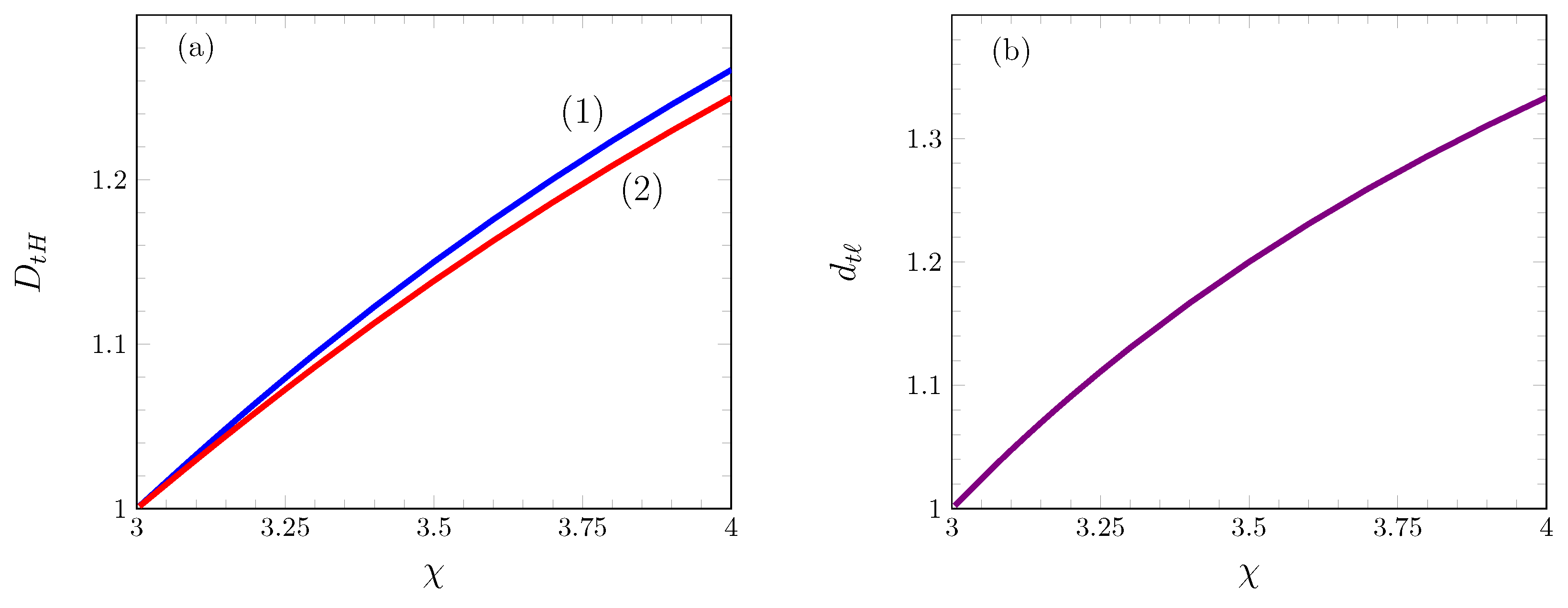
where is given by Equation (17). The graphs of versus for and are shown in Figure 3a. It contrast to the topological fractal dimension, the topological connectivity dimension is independent of the lattice dimension d and is equal to
The graph of versus is shown in Figure 3b. The general property that the topological connectivity dimension can be either equal to or less than the topological dimension of the fractal network implies that the scale-free fracture network models have the topological dimension in two as well as in three dimensions.
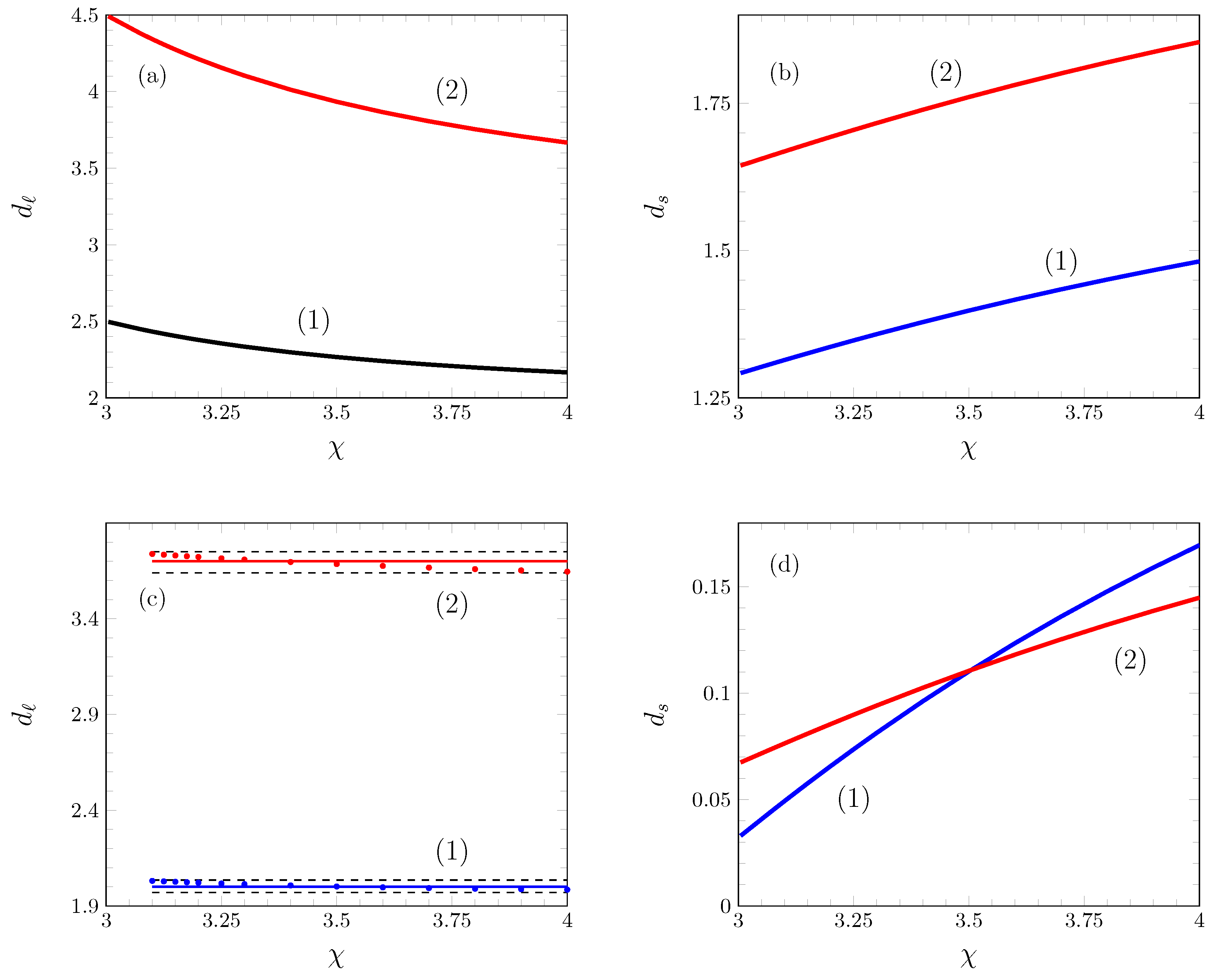
The fractal dimension of the critical percolation cluster (representing the fracture network model) is determined by the first scaling relation in Equation (15). Accordingly, from Equations (13) and (17), the fractal dimension of the scale-free fracture network model is equal to
Figure 4a shows the graphs of connectivity dimension for the scale-free fracture network model as the functions of for and .
The transport properties of the fractal fracture network are strongly dependent on the numbers of effective spatial and dynamical degrees of freedom of walkers in the network [45,46,47,48]. The number of effective dynamical degrees of freedom is equal to the network spectral dimension. The admissible values of the spectral dimension are bound in the range of [41]. However, explicit expressions for the network spectral dimension are known only for a few kinds of fractal networks. However, it was argued [48] that the spectral dimension of the fractal network can be approximately estimated using the following empirical relation
The graphs of versus calculated with the help of Equation (21) together with Equations (17), (18), and (20) are shown in Figure 4b. Notice that the spectral dimensions of the scale-free fracture networks are always less than 2, and so the fractal dimension of the random walk is . This means that the random walks in fracture networks are recurrent. By following the arguments from Ref. [77], we find that the number of effective spatial degrees of freedom in the critical percolation cluster formed in the scale-free network embedded in d-dimensional lattice is equal to
which differs from the relation derived in [77] in view of the unusual condition . Surprisingly, we establish that the scale-free fracture network models are characterized by the universal numbers of effective spatial degrees of freedom determined by the network-embedding dimension. Specifically, we found that in and in , independently of the degree distribution exponent varying in the range of (see Figure 4c). Conversely, the index of network loopiness defined by Equation (12) increases with the increase in degree distribution exponent , as shown in Figure 4d.
5. Conclusions
In this work, we put forward two kinds of models for fractal fracture networks in two and three dimensions. The first kind of models is based on the Bernoulli percolation of line slots in regular lattices. The second one explores the site percolation in scale-free networks embedded in the two- and three-dimensional lattices. The inherent fractal features and key attributes of model fracture networks are outlined.
The numerical simulations of the slot percolation model reveal that the fracture network porosity decreases with increase in the slot length. Nonetheless, we found that the critical exponents and the fractal attributes of the critical percolation cluster are independent of the slot length. In order to model the power-law distribution of crack lengths in the fracture network, we perform the numerical simulations of the slot percolation model with the power-law distribution of the slot lengths. We found that the crack length distribution exponent characterizing the fracture network model is larger than the slot length distribution exponent. We also noted that the fractal dimension of the minimum path and other fractal attributes of the fracture network model are dependent on the slot length distribution exponent. A more detailed analysis of these observations will be reported elsewhere after completing a comprehensive set of Monte Carlo simulations.
On the other hand, we suggest that the scale-free fracture networks is modeled within a framework of site percolation on the scale-free networks embedded in two- and three-dimensional lattices. With this model, the effects of degree distribution on other fractal features of the model fracture networks are analytically revealed. In particular, we established the expressions for the fractal, the connectivity, the topological fractal, and the spectral dimensions in the terms of the degree distribution exponent and the embedding dimension. Thus, by varying the degree distribution exponent, one can model the scale-free fracture networks with a predesigned set of dimension numbers. Surprisingly, we found that the scale-free fracture network models are characterized by the universal numbers of effective spatial degrees of freedom which are determined by the dimension of the embedding lattice.
In summary, this work focused on the topological features of the fractal models of fracture networks. Our findings provide a novel insight into the modeling of fractal fracture networks. The ultimate aim of the fracture network modeling is to predict or reproduce the transport and storage properties of different fracture systems. Accordingly, the effects of the fractal features of the model networks on the transport phenomena and storage capacity will be the subject of forthcoming studies.
Author Contributions
Writing—original draft preparation, H.M.-N.; Writing—review and editing, D.S. and B.M.; Conceptualization, A.S.B.; Methodology, D.S. and B.M.; Software, D.S.; Formal analysis, H.M.-N. and A.S.B.; Visualization, H.M.-N. and D.S.; Supervision, A.S.B. All authors have read and agreed to the published version of the manuscript.
Funding
This research was sponsored by the Instituto Politécnico Nacional Project under grants SIP 20231303 and 20230048.
Data Availability Statement
All data are contained within the paper, and a report of any other data is not included.
Conflicts of Interest
The authors declare no conflict of interest.
References
- Caddick, J.; Piperi, T.; Tomé, C.M.; Ruchonnet, C.; Hashim, N.; Turner, M.; Plampton, W.; Dimabuyu, A.J.; Betty, W.X.J.; Reilly, T.; et al. Global Overview of Fractured Basement Plays. Pet. Coal 2020, 62, 1180–1208. [Google Scholar]
- Troeger, U.; Chambel, A. Topical Collection: Progress in fractured-rock hydrogeology. Hydrogeol. J. 2021, 29, 2557–2560. [Google Scholar] [CrossRef]
- Hunt, A.G.; Sahimi, M. Flow, Transport, and Reaction in Porous Media: Percolation Scaling, Critical-Path Analysis, and Effective Medium Approximation. Rev. Geophys. 2017, 55, 993–1078. [Google Scholar] [CrossRef]
- Zhang, T.; Sun, S.; Song, H. Flow Mechanism and Simulation Approaches for Shale Gas Reservoirs: A Review. Transp. Porous Media 2019, 126, 655–681. [Google Scholar] [CrossRef] [Green Version]
- Gao, Y.; Rahman, M.M.; Lu, J. Novel Mathematical Model for Transient Pressure Analysis of Multifractured Horizontal Wells in Naturally Fractured Oil Reservoir. ACS Omega 2021, 6, 15205–15221. [Google Scholar] [CrossRef] [PubMed]
- Wei, Y.; Wang, J.; Yu, W.; Qi, Y.; Miao, J.; Yuan, H.; Liu, C. A smart productivity evaluation method for shale gas wells based on 3D fractal fracture network model. Pet. Explor. Dev. 2021, 48, 911–922. [Google Scholar] [CrossRef]
- Anders, M.H.; Laubach, S.E.; Scholz, C.H. Microfractures: A review. J. Struct. Geol. 2014, 69, 377–394. [Google Scholar] [CrossRef] [Green Version]
- Santiago, E.; Velasco-Hernández, J.X.; Romero-Salcedo, M. A descriptive study of fracture networks in rocks using complex network metrics. Comput. Geosci. 2016, 88, 97–114. [Google Scholar] [CrossRef]
- Peacock, D.C.P.; Nixon, C.W.; Rotevatn, A.; Sanderson, D.J.; Zuluaga, L.F. Glossary of fault and other fracture networks. J. Struct. Geol. 2016, 92, 12–29. [Google Scholar] [CrossRef]
- Long, J.C.S.; Remer, J.S.; Wilson, C.R.; Witherspoon, P.A. Porous media equivalents for networks of discontinuous fractures. Water Resour. Res. 1982, 18, 645–658. [Google Scholar] [CrossRef] [Green Version]
- Wei, W.; Xia, Y. Geometrical, fractal and hydraulic properties of fractured reservoirs: A mini-review. Adv. Geo-Energy Res. 2017, 1, 31–38. [Google Scholar] [CrossRef] [Green Version]
- Huseby, O.; Thovert, J.F.; Adler, P.M. Geometry and topology of fracture systems. J. Phys. A Math. Gen. 1997, 30, 1415–1444. [Google Scholar] [CrossRef]
- Adler, P.M.; Thovert, J.F. Fractures and Fracture Networks, Theory and Applications of Transport in Porous Media; Springer: Dordrecht, The Netherlands, 1999. [Google Scholar]
- Zeeb, C.; Gomez-Rivas, E.; Bons, P.D.; Blum, P. Evaluation of sampling methods for fracture network characterization using outcrops. AAPG Bull. 2013, 97, 1545–1566. [Google Scholar] [CrossRef]
- Estrada, E.; Sheerin, M. Random neighborhood graphs as models of fracture networks on rocks: Structural and dynamical analysis. Appl. Math. Comput. 2017, 314, 360–379. [Google Scholar] [CrossRef] [Green Version]
- Esser, S.; Lower, E.; Peuker, U.A. Network model of porous media – Review of old ideas with new methods. Sep. Purif. Technol. 2021, 257, 117854. [Google Scholar] [CrossRef]
- Healy, D.; Rizzo, R.E.; Cornwell, D.G.; Farrel, N.J.C.; Watkins, H.; Timms, N.E.; Gomez-Rivas, E.; Smith, M. FracPaQ: A MATLABTM toolbox for the quantification of fracture patterns. J. Struct. Geol. 2017, 95, 1–16. [Google Scholar] [CrossRef] [Green Version]
- Yang, B.; Liy, Y. Application of Fractals to Evaluate Fractures of Rock Due to Mining. Fractal Fract 2022, 6, 96. [Google Scholar] [CrossRef]
- Bonnet, E.; Bour, O.; Odling, N.E.; Davy, P.; Main, I.; Cowie, P.; Berkowitz, B. Scaling of fracture systems in geological media. Rev. Geophys. 2001, 39, 347–383. [Google Scholar] [CrossRef] [Green Version]
- Wu, Y.; Tahmasebi, P.; Lin, C.; Zahid, M.A.; Dong, C.; Golab, A.N.; Ren, L. A comprehensive study on geometric, topological and fractal characterizations of pore systems in low-permeability reservoirs based on SEM, MICP, NMR, and X-ray CT experiments. Mar. Pet. Geol. 2019, 103, 12–28. [Google Scholar] [CrossRef]
- Babadagli, T. Unravelling transport in complex natural fractures with fractal geometry: A comprehensive review and new insights. J. Hydrol. 2020, 587, 124937. [Google Scholar] [CrossRef]
- Jafari, A.; Babadagli, T. Estimation of equivalent fracture network permeability using fractal and statistical network properties. J. Pet. Sci. Eng. 2012, 92–93, 110–123. [Google Scholar] [CrossRef]
- Ghanbarian, B.; Hunt, A.G.; Skaggs, T.H.; Jarvis, N. Upscaling soil saturated hydraulic conductivity from pore throat characteristics. Adv. Water Resour. 2017, 104, 105–113. [Google Scholar] [CrossRef] [Green Version]
- Thanh, L.D.; Jougnot, D.; Van Do, P.; Mendieta, A.; Ca, N.X.; Hoa, V.X.; Tan, P.M.; Hien, N.T. Electroosmotic Coupling in Porous Media, a New Model Based on a Fractal Upscaling Procedure. Transp. Porous Media 2020, 134, 249–274. [Google Scholar] [CrossRef]
- Zhang, X.; Ma, F.; Yin, S.; Wallace, C.D.; Soltanian, M.R.; Dai, Z.; Ritzi, R.W.; Ma, Z.; Zhan, C.; Lü, X. Application of upscaling methods for fluid flow and mass transport in multi-scale heterogeneous media: A critical review. Appl. Energy 2021, 303, 117603. [Google Scholar] [CrossRef]
- Xu, P. A discussion on fractal models for transport physics of porous media. Fractals 2015, 25, 1530001. [Google Scholar] [CrossRef]
- Xu, P.; Li, C.; Qiu, S.; Sasmito, A.P. A fractal network model for fractured porous media. Fractals 2016, 24, 1650018. [Google Scholar] [CrossRef]
- Maillot, J.; Davy, P.; Le Goc, R.; Darcel, C.; de Dreuzy, J.R. Connectivity, permeability, and channeling in randomly distributed and kinematically defined discrete fracture network models. Water Resour. Res. 2016, 52, 8526–8545. [Google Scholar] [CrossRef] [Green Version]
- Cai, J.; Wei, W.; Hu, X.; Liu, R.; Wang, J. Fractal characterization of dynamic fracture network extension in porous media. Fractals 2017, 25, 1750023. [Google Scholar] [CrossRef]
- Wang, W.D.; Su, Y.L.; Zhang, Q.; Xiang, G.; Cui, S.M. Performance-based fractal fracture model for complex fracture network simulation. Pet. Sci. 2018, 15, 126–134. [Google Scholar] [CrossRef] [Green Version]
- Zhu, J. Effective aperture and orientation of fractal fracture network. Phys. A 2018, 512, 27–37. [Google Scholar] [CrossRef]
- Zhang, L.; Cui, C.; Ma, X.; Sun, Z.; Liu, F.; Zhang, K. A fractal discrete fracture network model for history matching of naturally fractured reservoirs. Fractals 2019, 27, 1940008. [Google Scholar] [CrossRef]
- Zhu, X.; Liu, G.; Gao, F.; Ye, D.; Luo, J. A Complex Network Model for Analysis of Fractured Rock Permeability. Adv. Civ. Eng. 2020, 2020, 8824082. [Google Scholar] [CrossRef]
- Li, Y.L.; Feng, M. Analysis of flow resistance in fractal porous media based on a three-dimensional pore-throat model. Therm. Sci. Eng. Prog. 2021, 22, 100833. [Google Scholar] [CrossRef]
- Li, W.; Zhao, H.; Wu, H.; Wang, L.; Sun, W.; Ling, X. A novel approach of two-dimensional representation of rock fracture network characterization and connectivity analysis. J. Pet. Sci. Eng. 2020, 184, 106507. [Google Scholar] [CrossRef]
- Stoll, M.; Huber, F.M.; Trumm, M.; Enzmann, F.; Meinel, D.; Wenka, A.; Schill, E.; Schäfer, T. Experimental and numerical investigations on the effect of fracture geometry and fracture aperture distribution on flow and solute transport in natural fractures. J. Contam. Hydrol. 2019, 221, 82–97. [Google Scholar] [CrossRef]
- Fu, J.; Thomas, H.R.; Li, C. Tortuosity of porous media: Image analysis and physical simulation. Earth-Sci. Rev. 2021, 212, 103439. [Google Scholar] [CrossRef]
- Roy, A.; Perfect, E.; Dunne, W.M.; McKay, L.D. Fractal characterization of fracture networks: An improved box-counting technique. J. Geophys. Res. 2007, 112, B12201. [Google Scholar] [CrossRef]
- Wei, D.J.; Liu, Q.; Zhang, H.X.; Hu, Y.; Deng, Y.; Mahadevan, S. Box-covering algorithm for fractal dimension of weighted networks. Sci. Rep. 2013, 3, 3049. [Google Scholar] [CrossRef] [Green Version]
- de Sá, L.A.P.; Zielinski, K.M.C.; Rodrigues, É.O.; Backes, A.R.; Florindo, J.B.; Casanova, D. A novel approach to estimated Boulingand-Minkowski fractal dimension from complex networks. Chaos Solitons Fractals 2022, 157, 111894. [Google Scholar] [CrossRef]
- Balankin, A.S.; Patino-Ortiz, J.; Patino-Ortiz, M. Inherent features of fractal sets and key attributes of fractal models. Fractals 2022, 30, 2250082. [Google Scholar] [CrossRef]
- Collon, P.; Bernasconi, D.; Vuilleumier, C.; Renard, P. Statistical metrics for the characterization of karst network geometry and topology. Geomorphology 2017, 283, 122–142. [Google Scholar] [CrossRef] [Green Version]
- Jin, Y.; Wang, C.; Liu, S.; Quan, W.; Liu, X. Systematic definition of complexity assembly in fractal porous media. Fractals 2020, 28, 2050079. [Google Scholar] [CrossRef]
- Ammari, A.; Abbes, C.; Abida, H. Geometric properties and scaling laws of the fracture network of the Ypresian carbonate reservoir in central Tunisia: Examples of Jebels Ousselat and Jebil. J. Afr. Earth Sci. 2022, 196, 104718. [Google Scholar] [CrossRef]
- Balankin, A.S. The topological Hausdorff dimension and transport properties of Sierpinski carpets. Phys. Lett. A 2017, 381, 2801–2808. [Google Scholar] [CrossRef]
- Balankin, A.S.; Valivia, J.C.; Marquez, J.; Susarrey, O.; Solorio-Avila, M.A. Anomalous diffusion of fluid momentum and Darcy-like law for laminar flow in media with fractal porosity. Phys. Lett. A 2018, 2380, 2767–2773. [Google Scholar] [CrossRef]
- Chen, K.; Liang, F.; Wang, C. A fractal hydraulic model for water retention and hydraulic conductivity considering adsorption and capillarity. J. Hydrol. 2021, 602, 126763. [Google Scholar] [CrossRef]
- Balankin, A.S.; Ramírez-Joachin, J.; Gonzalez-Lopez, G.; Gutíerrez-Hernandez, S. Formation factors for a class of deterministic models of pre-fractal pore-fracture networks. Chaos Solitons Fractals 2022, 162, 112452. [Google Scholar] [CrossRef]
- Feng, S.; Wang, H.; Cui, Y.; Ye, Y.; Liu, Y.; Li, X.; Wang, H.; Yang, R. Fractal discrete fracture network model for the analysis of radon migration in fractured media. Comput. Geotech. 2020, 128, 103810. [Google Scholar] [CrossRef]
- Ghanbarian, B.; Perfect, E.; Liu, H.H. A geometrical aperture–width relationship for rock fractures. Fractals 2019, 27, 1940002. [Google Scholar] [CrossRef] [Green Version]
- Hooker, J.N.; Laubach, S.E.; Marrett, R. Microfracture spacing distributions and the evolution of fracture patterns in sandstones. J. Struct. Geol. 2018, 108, 66–79. [Google Scholar] [CrossRef]
- Ni, C.; Liu, C.; Zhang, S.; Fu, C. 3D Simulation of Rock Fractures Distribution in Gaosong Field, Gejiu Ore District. In Proceedings of the 2nd International Conference on Green Communications and Networks 2012 (GCN 2012): Volume 1; Yang, Y., Ma, M., Eds.; Lecture Notes in Electrical Engineering; Springer: Berlin/Heidelberg, Germany, 2023; Volume 223. [Google Scholar] [CrossRef]
- Develi, K.; Babadagly, T.; Comlekci, C. A new computer-controlled surface-scanning device for measurement of fracture surface roughness. Comput. Geosci. 2001, 27, 265–277. [Google Scholar] [CrossRef]
- Revil, A.; Binley, A.; Mejus, L.; Kessouri, P. Predicting permeability from the characteristic relaxation time and intrinsic formation factor of complex conductivity spectra. Water Resour. Res 2015, 51, 6672–6700. [Google Scholar] [CrossRef] [Green Version]
- Andresen, C.A.; Hansen, A.; Le Goc, R.; Davy, P.; Hope, S.M. Topology of fracture networks. Front. Phys 2013, 1, 7. [Google Scholar] [CrossRef] [Green Version]
- Davy, P.; Le Goc, R.; Darcel, C.; Bour, O.; de Dreuzy, J.R.; Munier, R. A likely universal model of fracture scaling and its consequence for crustal hydromechanics. J. Geophys. Res. Solid Earth 2010, 115, B10411. [Google Scholar] [CrossRef]
- Odling, N.E. Scaling and connectivity of joint systems in sandstones from western Norway. J. Struct. Geol. 1997, 19, 1257–1271. [Google Scholar] [CrossRef]
- Lavoine, E.; Davy, P.; Darcel, C.; Le Goc, R. On the Density Variability of Poissonian Discrete Fracture Networks, with application to power-law fracture size distributions. Adv. Geosci. 2019, 49, 77–83. [Google Scholar] [CrossRef] [Green Version]
- Davy, P.; Goc, R.L.; Darcel, C. A model of fracture nucleation, growth and arrest, and consequences for fracture density and scaling. J. Geophys. Res. Solid Earth 2013, 118, 1393–1407. [Google Scholar] [CrossRef] [Green Version]
- Sebők, D.; Vásárhelyi, L.; Szenti, I.; Vajtai, R.; Kónya, Z.; Kukovecz, Á. Fast and accurate lacunarity calculation for large 3D micro-CT datasets. Acta Mater. 2021, 214, 116970. [Google Scholar] [CrossRef]
- Scott, R.; Kadum, H.; Salmaso, G.; Calaf, M.; Cal, R.B. A Lacunarity-Based Index for Spatial Heterogeneity. Earth Space Sci. 2022, 9, e2021EA002180. [Google Scholar] [CrossRef]
- Cojocaru, J.I.R.; Popescu, D.; Nicolae, I.E. Texture classification based on succolarity. In Proceedings of the 21st Telecommunications Forum Telfor, Belgrade, Serbia, 26–28 November 2013; pp. 1–5. [Google Scholar] [CrossRef]
- Sahu, A.K.; Roy, A. Clustering, Connectivity and Flow Responses of Deterministic Fractal-Fracture Networks. Adv. Geosci. 2020, 54, 149–156. [Google Scholar] [CrossRef]
- de Melo, R.H.C.; Conci, A. How Succolarity could be used as another fractal measure in image analysis. Telecommun. Syst. 2013, 52, 1643–1655. [Google Scholar] [CrossRef]
- Bour, O.; Davy, P. On the connectivity of three-dimensional fault networks. Water Resour. Res. 1998, 34, 2611–2622. [Google Scholar] [CrossRef]
- Roy, A.; Perfect, E.; Dunne, W.M.; Odling, N.; Kim, J.W. Lacunarity analysis of fracture networks: Evidence for scale-dependent clustering. J. Struct. Geol. 2010, 32, 1444–1449. [Google Scholar] [CrossRef]
- Wu, H.; Pollard, D.D. Imaging 3-D fracture networks around boreholes. AAPG Bull. 2002, 86, 593–604. [Google Scholar] [CrossRef]
- Cai, J.; Zhang, Z.; Wei, W.; Guo, D.; Li, S.; Zhao, P. The critical factors for permeability-formation factor relation in reservoir rocks: Pore-throat ratio, tortuosity and connectivity. Energy 2019, 188, 116051. [Google Scholar] [CrossRef]
- Sundberg, K. Effect of impregnating waters on electrical conductivity of soils and rocks. Trans. Am. Inst. Min. Metall. Petrol. Eng. 1932, 97, 367–391. [Google Scholar]
- Archie, G.E. The electrical resistivity log as an aid in determining some reservoir characteristics. Petrol. Trans. AIME 1942, 146, 54–62. [Google Scholar] [CrossRef]
- Bourbatache, M.K.; Bennai, F.; Zhao, C.F.; Millet, O.; Aït-Mokhtar, A. Determination of geometrical parameters of the microstructure of a porous medium: Application to cementitious materials. Int. Comm. Heat Mass Transf. 2020, 117, 104786. [Google Scholar] [CrossRef]
- Cai, J.; Wei, W.; Hu, X.; Wood, D.A. Electrical conductivity models in saturated porous media: A review. Earth Sci. Rev. 2017, 171, 419–433. [Google Scholar] [CrossRef]
- Zhong, Z.; Rezaee, R.; Esteban, L.; Josh, M.; Feng, R. Determination of Archie’s cementation exponent for shale reservoirs; an experimental approach. J. Petrol. Sci. Eng. 2021, 201, 108527. [Google Scholar] [CrossRef]
- Siddiqui, S.; Soldati, M.; Castaldini, D. Appraisal of active deformation from drainage network and faults: Inferences from non-linear analysis. Earth Sci. Inform. 2015, 8, 233–246. [Google Scholar] [CrossRef] [Green Version]
- Xia, Y.; Cai, J.; Perfect, E.; Wei, W.; Zhang, Q.; Meng, Q. Fractal dimension, lacunarity and succolarity analyses on CT images of reservoir rocks for permeability prediction. J. Hydrol. 2019, 579, 124198. [Google Scholar] [CrossRef]
- Balankin, A.S. A continuum framework for mechanics of fractal materials I: From fractional space to continuum with fractal metric. Eur. Phys. J. B 2015, 88, 90. [Google Scholar] [CrossRef]
- Balankin, A.S. Effective degrees of freedom of a random walk on a fractal. Phys. Rev. E 2015, 92, 062146. [Google Scholar] [CrossRef]
- Balankin, A.S.; Martínez-Cruz, M.A.; Álvarez-Jasso, M.D.; Patiño-Ortiz, M.; Patiño-Ortiz, J. Effects of ramification and connectivity degree on site percolation threshold on regular lattices and fractal networks. Phys. Lett. A 2019, 383, 957–966. [Google Scholar] [CrossRef]
- Balankin, A.S. Fractional space approach to studies of physical phenomena on fractals and in confined low-dimensional systems. Chaos Solitons Fractals 2020, 132, 10957. [Google Scholar] [CrossRef]
- McCaffrey, K.J.W.; Holdsworth, R.E.; Pless, J.; Franklin, B.S.G.; Hardman, K. Basement reservoir plumbing: Fracture aperture, length and topology analysis of the Lewisian Complex, NW Scotland. J. Geol. Soc. 2020, 177, 1281–1293. [Google Scholar] [CrossRef]
- Cao, M.; Hirose, S.; Sharma, M.M. Factors controlling the formation of complex fracture networks in naturally fractured geothermal reservoirs. J. Pet. Sci. Eng. 2022, 208, 109642. [Google Scholar] [CrossRef]
- Liu, X.; Jin, Y.; Lin, B.; Zhang, Q.; Wei, S. An integrated 3D fracture network reconstruction method based on microseismic events. J. Nat. Gas Sci. Eng. 2021, 95, 104182. [Google Scholar] [CrossRef]
- Babadagli, T. Fractal analysis of 2D fracture networks of geothermal reservoirs in south-western Turkey. J. Volcanol. Geotherm. Res. 2001, 112, 83–103. [Google Scholar] [CrossRef]
- Liu, R.; Zhu, T.; Jiang, Y.; Li, B.; Yu, L.; Du, Y.; Wang, Y. A predictive model correlating permeability to two-dimensional fracture network parameters. Bull. Eng. Geol. Environ. 2019, 78, 1589–1605. [Google Scholar] [CrossRef]
- Vega, B.; Kovscek, A.R. Fractal Characterization of Multimodal, Multiscale Images of Shale Rock Fracture Networks. Energies 2022, 15, 1012. [Google Scholar] [CrossRef]
- Ozkaya, S.I.; Al-Fahmi, M.M. Estimating size of finite fracture networks in layered reservoirs. Appl. Comput. Geosci. 2022, 15, 100089. [Google Scholar] [CrossRef]
- Sanderson, D.J.; Peacock, D.C.P.; Nixon, C.W.; Rotevatn, A. Graph theory and the analysis of fracture networks. J. Struct. Geol. 2019, 125, 155–165. [Google Scholar] [CrossRef] [Green Version]
- Phillips, J.D.; Schwanghart, W.; Heckmann, T. Graph theory in the geosciences. Earth-Sci. Rev. 2015, 143, 147–160. [Google Scholar] [CrossRef]
- Perrier, E.M.A.; Bird, N.R.A.; Rieutord, T.B. Percolation properties of 3-D multiscale pore networks: How connectivity controls soil filtration processes. Biogeosciences 2010, 7, 3177–3186. [Google Scholar] [CrossRef] [Green Version]
- Hunt, A.; Ewing, R.; Ghanbarian, B. Percolation Theory for Flow in Porous Media; Springer: Berlin/Heidelberg, Germany, 2014. [Google Scholar]
- Liua, J.; Regenauer-Lieb, K. Application of percolation theory to microtomography of rocks. Earth-Sci. Rev. 2021, 214, 103519. [Google Scholar] [CrossRef]
- Yin, T.; Man, T.; Galindo-Torres, S.A. Universal scaling solution for the connectivity of discrete fracture networks. Phys. A 2022, 599, 127495. [Google Scholar] [CrossRef]
- Vevatne, J.N.; Rimstad, E.; Hope, S.M.; Korsnes, R.; Hansen, A. Fracture networks in sea ice. Front. Phys. 2014, 2, 21. [Google Scholar] [CrossRef] [Green Version]
- Liu, Z. Study on the degree distribution properties of soil crack. IOP Conf. Ser. Earth Environ. Sci. 2019, 289, 012007. [Google Scholar] [CrossRef]
- Balankin, A.S.; Mena, B.; Martínez-Cruz, M.A. Topological Hausdorff dimension and geodesic metric of critical percolation cluster in two dimensions. Phys. Lett. A 2017, 381, 2665–2672. [Google Scholar] [CrossRef]
- Xu, C.; Dowd, P.A.; Mardia, K.V.; Fowell, R.J. A Connectivity Index for Discrete Fracture Networks. Math. Geol. 2006, 38, 611–634. [Google Scholar] [CrossRef]
- Costa, L.F.; Rodrigues, F.A.; Travieso, G.; Boas, P.R.V. Characterization of complex networks: A survey of measurements. Adv. Phys. 2007, 56, 167–242. [Google Scholar] [CrossRef] [Green Version]
- Rozenfeld, A.F.; Cohen, R.; ben-Avraham, D.; Havlin, S. Scale-Free Networks on Lattices. Phys. Rev. Lett. 2002, 89, 218701. [Google Scholar] [CrossRef] [PubMed] [Green Version]
- Warren, C.P.; Sander, L.M.; Sokolov, I.M. Geography in a scale-free network model. Phys. Rev. E 2002, 66, 056105. [Google Scholar] [CrossRef] [Green Version]
- Hestir, K.; Long, J.C.S. Analytical expressions for the permeability of random two- dimensional Poisson fracture networks based on regular lattice percolation and equivalent media theories. J. Geophys. Res. 1990, 95, 21565. [Google Scholar] [CrossRef] [Green Version]
- Stauffer, D.; Aharony, A. Introduction to Percolation Theory, 2nd ed.; Taylor and Francis: London, UK, 1994. [Google Scholar] [CrossRef]
- Li, M.; Liu, R.R.; Lü, L.; Hua, M.B.; Xu, S.; Zhang, Y.C. Percolation on complex networks: Theory and application. Phys. Rep. 2021, 907, 1–68. [Google Scholar] [CrossRef]
- Cruz, M.-Á.M.; Ortiz, J.P.; Ortiz, M.P.; Balankin, A. Percolation on Fractal Networks: A Survey. Fractal Fract. 2023, 7, 231. [Google Scholar] [CrossRef]
- Rodriguez, A.A.; Medina, E. Analytical results for random line networks applications to fracture networks and disordered fiber composites. Phys. A 2000, 282, 35–49. [Google Scholar] [CrossRef]
- Mourzenko, V.V.; Thovert, J.-F.; Adler, P.M. Macroscopic permeability of three-dimensional fracture networks with power-laws size distribution. Phys. Rev. E 2004, 69, 066307. [Google Scholar] [CrossRef]
- Khamforoush, K.; Shams, K.; Thovert, J.-F.; Adler, P.M. Permeability and percolation of anisotropic three-dimensional fracture networks. Phys. Rev. E 2008, 77, 056307. [Google Scholar] [CrossRef] [PubMed]
- Cohen, R.; ben-Avraham, D.; Havlin, S. Percolation critical exponents in scale-free networks. Phys. Rev. E 2002, 66, 036113. [Google Scholar] [CrossRef] [PubMed] [Green Version]
- Cohen, R.; Havlin, S. Fractal dimensions of percolating networks. Phys. A 2004, 336, 6–13. [Google Scholar] [CrossRef]
- Hooyberghs, H.; Van Schaeybroeck, B.; Moreira, A.A.; Andrade, J.S.; Herrmann, H.J.; Indekeu, J.O. Biased percolation on scale-free networks. Phys. Rev. E 2010, 81, 011102. [Google Scholar] [CrossRef] [Green Version]
- Leroyer, Y.; Pommiers, E. Monte Carlo analysis of percolation of line segments on a square lattice. Phys. Rev. B 1994, 50, 2795–2799. [Google Scholar] [CrossRef] [Green Version]
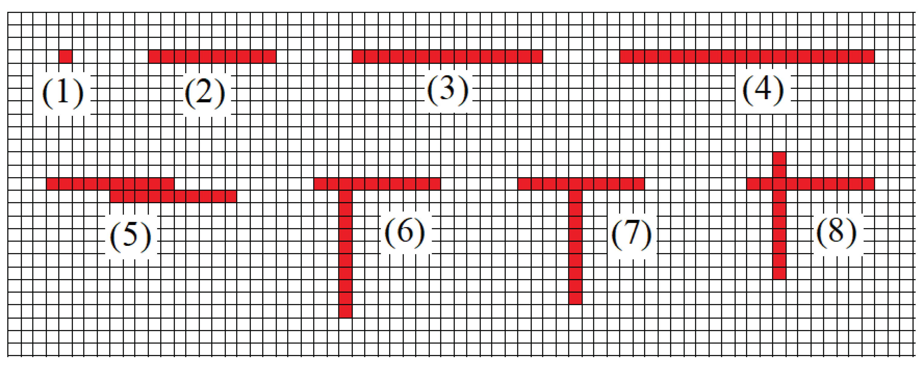
Figure 1.
Illustration of rules for the slot percolation model on square lattice: open site (1); straight slot of length (2); crack of length formed by two overlapping slots (3); crack of length formed by contact between two slots (4); crack with a variable width formed by contact between two slots (5); vertices formed by: contact between two slots (6) and two overlapping slots (7); and the crossing of two slots (8).

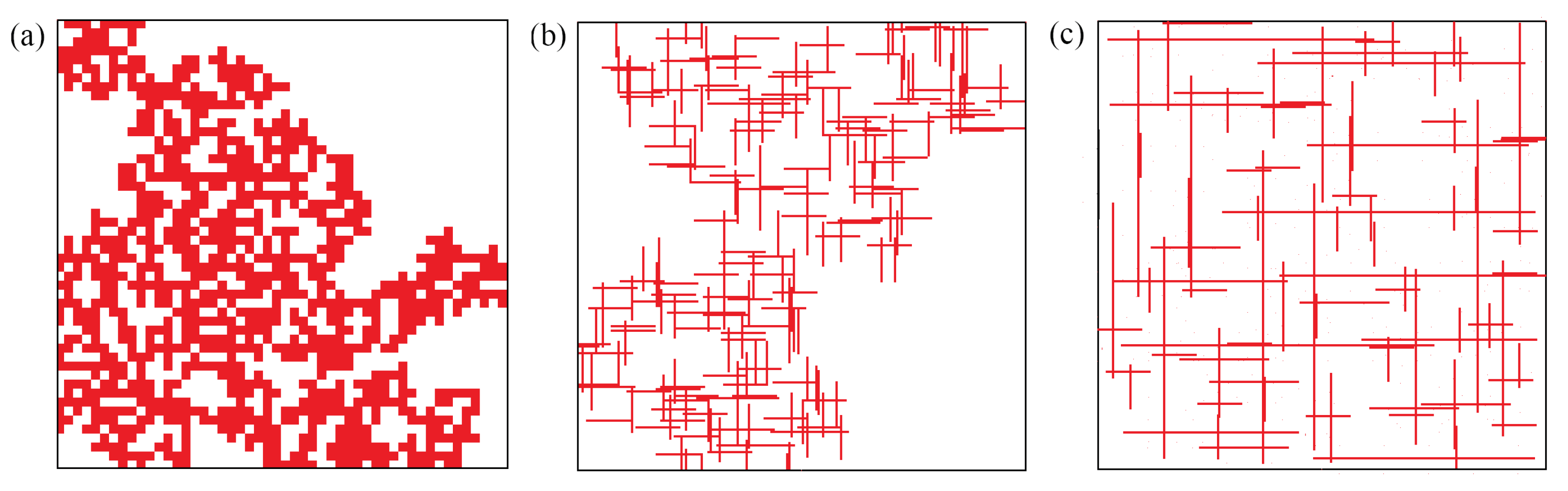
Figure 2.
Percolation clusters on a square lattice obtained in numerical simulations on the square lattice with the edge size for: (a) site percolation; (b) percolation of straight slots of fixed length ; (c) percolation of straight slots with the power-law length distribution defined by Equation (16) with , and .

Figure 3.
Graphs of: (a) topological fractal dimension versus degree distribution exponent for (1) and (2) calculated by Equation (18) together with Equation (17); (b) topological connectivity dimension versus degree distribution exponent calculated by Equation (19).

Figure 4.
Graphs of: (a) connectivity dimension versus degree distribution exponent for (1) and (2) calculated by Equation (19); (b) spectral dimension versus degree distribution exponent for (1) and (2) calculated with the help of Equation (21) together with Equations (17) and (18); (c) number of effective spatial degrees of freedom versus the degree of the distribution exponent for (1) and (2) points are calculated using Equation (22), with given by Equation (19) and given by Equation (21), solid lines—the universal values in and in dashed lines denote the standard deviations of the estimated values of from the universal values; (d) fractal loopiness index versus degree distribution exponent for (1) and (2) calculated by Equation (12) together with Equations (20)–(22).

Table 2.
Dimension numbers and scaling exponents characterizing the fractal fracture networks.
| Parameter (Symbol) | Definition | ||
|---|---|---|---|
| Dimension numbers | Box-counting dimension | Box-counting dimension is defined via the scaling relation , where is the number of n-dimensional boxes of size r needed to cover the fracture network, while [76]. | |
| Topological fractal dimension | [41]. | ||
| Connectivity dimension | , where is the number of points connected with an arbitrary point inside of the -dimensional ball of radius ℓ around this point [76]. | ||
| Fractal dimension of the minimum path | The fractal dimension of the minimum path is defined via the scaling relation , where is the shortest distance between two randomly chosen points on the network, while r is the Euclidean distance between these points and denotes the ensemble average [76]. | ||
| Fractal dimension of geodesic lines | The fractal dimension of geodesic lines is equal to [79]. | ||
| Number of effective spatial degrees of freedom | The number of effective spatial degrees of freedom is the number of independent directions in which a random walker can move without violating any constraint imposed on it by the network topology [77]. | ||
| Number of effective dynamical degrees of freedom | The number of effective dynamical degrees of freedom is equal to the spectral dimension, which is commonly defined as , where is the probability that a random walker on the network returns to its origin after steps, while denotes the spatial average [79]. | ||
| Scaling exponents | Crack length distribution exponent | The crack length distribution exponent is defined via Equation (2). Commonly, it varies in the range of [56]. | |
| Crack roughness (Hurst) exponent | Roughness (Hurst) exponent is defined via the scaling behavior of the RMS roughness [53]. | ||
| Fracture aperture exponent | Fracture aperture exponent is defined by the scaling relation and varies in the range of [19,50]. | ||
| Network ramification exponent | The network ramification exponent is defined by Equation (7). | ||
| Degree distribution exponent | The degree distribution exponent is defined via Equation (10). | ||
| Fractal dimension of the random walk | The fractal dimension of the random walk is defined via the scaling behavior of the mean squared displacement of a random walker [77]. | ||
| Fractal dimension of the path tortuosity | The fractal dimension of the path tortuosity is defined via the scaling relation , where [48]. | ||
| Archie exponent | m | The Archie exponent is defined via Equation (6). | |
Disclaimer/Publisher’s Note: The statements, opinions and data contained in all publications are solely those of the individual author(s) and contributor(s) and not of MDPI and/or the editor(s). MDPI and/or the editor(s) disclaim responsibility for any injury to people or property resulting from any ideas, methods, instructions or products referred to in the content. |
© 2023 by the authors. Licensee MDPI, Basel, Switzerland. This article is an open access article distributed under the terms and conditions of the Creative Commons Attribution (CC BY) license (https://creativecommons.org/licenses/by/4.0/).
Share and Cite
MDPI and ACS Style
Mondragón-Nava, H.; Samayoa, D.; Mena, B.; Balankin, A.S. Fractal Features of Fracture Networks and Key Attributes of Their Models. Fractal Fract. 2023, 7, 509. https://doi.org/10.3390/fractalfract7070509
AMA Style
Mondragón-Nava H, Samayoa D, Mena B, Balankin AS. Fractal Features of Fracture Networks and Key Attributes of Their Models. Fractal and Fractional. 2023; 7(7):509. https://doi.org/10.3390/fractalfract7070509
Chicago/Turabian StyleMondragón-Nava, Hugo, Didier Samayoa, Baltasar Mena, and Alexander S. Balankin. 2023. "Fractal Features of Fracture Networks and Key Attributes of Their Models" Fractal and Fractional 7, no. 7: 509. https://doi.org/10.3390/fractalfract7070509