

Qualitative and Quantitative Analysis of Fractional Dynamics of Infectious Diseases with Control Measures

1
Department of Mathematics, College of Science & Arts, King Abdulaziz University, Rabigh, Saudi Arabia
2
Department of Mathematics, University of Swabi, Swabi 23561, Pakistan
*
Author to whom correspondence should be addressed.
Fractal Fract. 2023, 7(5), 400; https://doi.org/10.3390/fractalfract7050400
Submission received: 25 March 2023
/
Revised: 7 May 2023
/
Accepted: 12 May 2023
/
Published: 15 May 2023
(This article belongs to the Special Issue Fractional Calculus and Nonlinear Analysis: Theory and Applications)
Abstract
:Infectious diseases can have a significant economic impact, both in terms of healthcare costs and lost productivity. This can be particularly significant in developing countries, where infectious diseases are more prevalent, and healthcare systems may be less equipped to handle them. It is recognized that the hepatitis B virus (HBV) infection remains a critical global public health issue. In this study, we develop a comprehensive model for HBV infection that includes vaccination and hospitalization through a fractional framework. It has been shown that the solutions of the recommended system of HBV infection are positive and bounded. We examine the steady states of the model and determine the basic reproduction number; denoted by . The qualitative and quantitative behavior of the model is demonstrated using mathematical skills and numerical techniques. It has been proved that the infection-free steady state of the system is locally asymptotically stable if and unstable otherwise. Furthermore, the Ulam–Hyers stability (UHS) of the recommended fractional models is investigated and the significant conditions are provided. We present an iterative technique to visualize the dynamical behavior of the system. We perform different simulations to illustrate the effect of different input factors on the solution pathways of the system of HBV infection to conceptualize the role of parameters in the control and prevention of the infection.
1. Introduction
Infectious diseases are infections brought on by organisms, often microscopic in size, such as bacteria, viruses, fungi, or parasites that are transferred from host to host either indirectly or directly. Hepatitis B is a dangerous liver disease among infectious diseases which results in cancer, scarring of the organ, and liver failure. This disease affects the entire world and is one of the dominant causes of mortality. A vaccination for this illness has been available since 1982 and is 95% effective [1]. About 80% of primary liver cancer cases are caused by this illness. About a quarter of all paediatric illnesses progress to chronic infections. In China, approximately 93 million individuals are affected by the infection of HBV [2]. This infection transmits from one person to another when they use infectious blood, infectious body fluids of infected individuals, and through contaminated tools including syringes and in operations, etc. [1,3]. A vertical sort of transmission occurs when a newborn infant becomes infected from their infected mother. Sometimes a person infected by the HBV has no symptoms, which leads them to a severe unstable status or even death. However, after two to five months, the HBV infection reveals its symptoms, moreover, liver cancer and cirrhosis are the main causes of HBV infection.
Mathematical models are very important tools for effective investigation of the transmission and management of any infectious disease. Many mathematicians and biologists have created different epidemic models to represent the transmission dynamics of HBV. Medley et al. [4] explored catastrophic behavior in the dynamics of HBV for the first time. The authors [5] proposed an important technique for controlling the infection. Pang et al. investigated a model with immunized class and some other controls to eradicate the HBV disease [3]. The occurrence of the HBV infection was modelled and investigated by researchers in China [6]. In [7], the authors studied and explored the CTL immunological responses using a mathematical model. In [8,9], the researchers constructed and investigated diffusion models for HBV infection with a time delay. Zhao et al. established a model for calculating the vaccination’s long-term effectiveness [10], while Khan et al. considered the consequences of migrants on the dynamics of the infection [11]. In [12], the authors formulated a model to investigate the dynamics of the infection in Xinjiang. In addition to this, several studies have been presented in the literature to provide effective control interventions for this infectious disease [13,14]. The authors in [15] introduced a model of HBV with the effect of heroin and provided some control measures through control theory. This viral infection is the leading cause of liver cancer and is responsible for over 780,000 deaths each year. In addition to this, HBV infection also imposes a significant economic burden, with the costs associated with treating HBV-related liver diseases and lost productivity estimated to be in the billions of dollars each year. Therefore, we aim to develop an epidemic model for the intricate transmission phenomena of the HBV infection that includes vaccination and medication administered during hospitalization, to explore how these strategies affect the transmission and prevalence of HBV, and how they can be optimized to achieve the greatest reduction in the disease burden.
Fractional calculus involves the use of non-integer derivatives and integrals. The application of fractional derivatives is becoming increasingly important in many fields, including physics, engineering, finance, and biology [16,17]. In physics and engineering, fractional derivatives are used to model and analyze complex systems that exhibit non-linear behavior, such as viscoelastic materials, signal processing, and control systems [18]. Fractional calculus provides a more accurate description of these systems compared to traditional integer-order calculus. It has been presented in the literature [19,20] that non-integer derivatives can accurately depict biological processes because of their inherent characteristics and non-local behavior. In this study, our objective is to construct an epidemic model that accurately represents the intricate transmission dynamics of HBV infection with the effect of vaccination and medication administered during hospitalization through a fractional framework. Furthermore, we aim to demonstrate how the dynamical behavior of the system is affected by various input factors and memory index. The purpose of this work is to highlight the most effective scenario for the prevention of HBV infection and to illustrate whether the fractional parameter may be utilized as a control parameter or not.
The remaining part of this paper is structured as follows: In Section 2, we provide the rudimentary theory and concepts of the Caputo fractional derivative. We construct an epidemic model of HBV infection with vaccination and medication through hospitalization in Section 3. The suggested dynamics of HBV infection is represented in a fractional framework for accurate outcomes. We investigate the epidemic model for its basic properties and determine the reproduction parameter . The local and global stability results are established in Section 4 of this work. We investigate the solution of the system and demonstrated the Ulam–Hyers stability in Section 5. The tracking path behavior of the model is illustrated in Section 6 through an iterative method. We also conceptualize the impact of different input factors on the dynamics of HBV infection. Finally, the ending remarks of the overall work are given in Section 7.
2. Theory of Fractional Calculus
Here, we will introduce the rudimentary ideas and terminology of fractional theory, which will be utilized for the analysis of the system. Additionally, it has several beneficial uses across a variety of scientific areas. The essential concepts of the fractional derivative (FD) of Liouville and Caputo, introduced in [21,22,23], are as follows:
Definition 1.
Let us take a function such that , then, the fractional integral of Liouville–Caputo (LC) is denoted by I and is given by
where is the order of the fractional derivative and r is assumed for time.
Definition 2.
Consider in a manner that ; then, the fractional derivative of in the LC form is denoted by and is
subject to the constraint that .
Lemma 1.
Let us take the setup described below
the above system has a solution given by
Theorem 1
([23]). Select X to be a Banach space and to be compact and continuous. Then, T has a fixed point if
is bounded.
3. Evaluation of the Model
To construct the dynamics of HBV, we indicate the total human population by , which is further distributed in seven different classes: susceptible, vaccinated, exposed, acutely infected, chronic HBV case, hospitalized, and recovered individuals, expressed by , , , , , , and , respectively.
The birth rate of newborn babies () generates the susceptible population of humans, and successfully immunized newborns (, where transfer to while the un-immunized newborn babies are expressed, with a factor q, as carriers of the HBV infection. In addition to this, the fraction of newborns joins the chronic class, members of which are not fully immunized. This population is decreased due to the effective contact of the susceptible individuals with the population that are infected with HBV at a rate , where , and are the different rates of transmission due to , , and ; moreover, the said portion moves to to generate the exposed class. The vaccinated people leave this class and join the vaccinated class at the rate . In addition, those vaccinated individuals who lost their immunity join the class at the rate . The rate of death which occurs naturally, is considered to be d in all epidemiological classes. The number of individuals in decreases by the transfer of exposed people to the acutely infected class at the rate and also the rate d. Similarly, the acutely infected population is decreased at the rate d and treatment rate . Furthermore, this class is also decreased by to and a portion , where , to the recovered class. The class is also joined by the hospitalized at a rate , which expresses medication failure in the hospitalized class. It is also reduced by the rate d and the rate of recovery , as well as by medication at . The hospitalized class is reduced by the rate d and recovery of individuals at the rate , as well as the incomplete rate of medication . Finally, the remaining two classes, of vaccination and recovered , are decreased by the death rate d. By utilizing all of this above-mentioned information about the dynamics of a life threatening infection, we have the following system of differential equations for the vaccinated and hospitalized classes. Consequently, all of the equations may be expressed as the nonlinear ODE system:
with
and
A fractional derivative is a generalization of an ordinary derivative that can capture the memory effects and long-range correlations present in complex biological phenomena and epidemics. One of the most important aspects of epidemic modeling is to accurately capture the dynamics of the spread of the disease over time. Fractional derivatives allow us to incorporate memory and non-local effects that are not accounted for in classical models. For example, the fractional derivative can model the non-exponential decay of infectiousness of a disease over time, which is a common characteristic of many epidemics.
Moreover, fractional derivatives have the capability to account for heterogeneity within populations, encompassing variations in susceptibility and contact rates among individuals. This becomes especially crucial when modeling the spread of diseases in populations characterized by diverse demographics. When it comes to data fitting and analysis, the fractional framework offers an additional parameter that enhances the flexibility of the epidemic system. For our study on HBV infection dynamics, we have opted to employ fractional derivatives to depict the intricacies of the system. Our objective is to investigate the impact of different input factors of HBV on the system and to examine whether the fractional derivative order can be utilized as a viable control parameter or not. Therefore, we represent our model through Caputo FD as
where is the order of the LC derivative and , moreover, system (6) becomes system (5) for . The theory of fractional calculus offers a wide range of practical applications and provides a more precise representation of the dynamics of biological phenomena compared to integer-order derivatives. In the recent literature, several new fractional operators have been introduced. Our future work aims to explore the dynamics of HBV infection with the help of these novel operators, and we will further investigate and compare the outcomes produced by these fractional operators. The results presented below are on the non-negativity of the solution of the above-mentioned HBV infection model (5).
Theorem 2.
The solutions of the recommended system (6) of HBV infection are non-negative and bounded for positive initial values of state variables.
Proof of Theorem 2.
To prove the non-negativity and boundedness of the solutions of the recommended fractional system (6) of HBV infection, we proceed as follows:
thus, the solutions of our fractional model of HBV infection are non-negative. To determine the boundedness of the solutions, we add all the equations of the system and obtain the following
From the above, we have
Further, we obtain the following through the properties of the Mittag–Leffler function [21]:
this implies that Thus, the solutions of the recommended fractional model (6) of HBV infection are non-negative and bounded.
□
Model Analysis
The steady states, reproduction number, and stability of the steady states of our model will be investigated in this subsection of the paper. Epidemic models have two meaningful steady states, namely, disease-free equilibrium (DFE) and endemic equilibrium (EE). The DFE is denoted by and is given by
Here, we determine the expressions for the basic reproduction number, symbolized by , with the help of the next generation method [24]. In our system of HBV infection, we have four infected compartments , and , thus , then we have
The spectral radius of is the reproduction number, given by
in which , and We represent
and
The EE of (5) is indicated by
where , and represent the endemic states of the state variables and are calculated as
In the next step, we determine the local stability of the DFE of our system of HBV infection.
Theorem 3.
If , then of the recommended HBV model presented in (5) is locally asymptotically stable .
Proof of Theorem 3.
The Jacobian matrix associated with the model, denoted by , evaluated around the FDE of system (6) is as follows:
where and the associated characteristic equation of is constructed as
Obviously, one of the eigenvalues is , which is a negative real number and obviously has a negative real part. The coefficients involved in the above Equation (8) are calculated as follows:
Clearly, if , then . Furthermore, the other will have a negative real part if Equation (8) follows the associated Routh–Hurtwiz criterion [25]. Hence, it can be concluded from the above calculations that the DFE is for if the associated Routh–Hurtwiz criterion holds.
□
4. Existence Theory
Here, the qualitative analysis of the recommended system (6) of HBV infection will be presented. We assumed the following:
then, system (6) of HBV infection, in view of the above, can be expressed as:
in which is the bounded time interval and
the aforementioned (10) comparable integral converts into:
The key steps for analyzing our suggested system are the following hypotheses:
- (A1) Constants , and are considered such that(A2) Constants , and , are assumed in a way thatIn this case, we define a map T on X as follows:
If the above A1 and A2 hold true, then there is at least one solution of (10). In the next step, we will examine the solution of our recommended system.
Theorem 4.
If A1 and A2 are satisfied, then the recommended system (6) of HBV infection has at least one solution.
Proof of Theorem 4.
We will apply Schaefer’s fixed-point theorem to demonstrate the result. The following steps are taken to prove the theorem.
- S1: We shall demonstrate the continuity of T in the first step. For this, we assume that is continuous for , which also means that is continuous. Here, take , in a way that . Further, take the following:
- This implies that the operator T is continuous, because is true as long as is continuous.
- S2: The boundedness of the operator T will be investigated in the second step. If we select any , then, we have
Here, we will prove the boundedness of , where S is a bounded subset of X. Then, for any , we have such that
Consequently, if we use the aforementioned condition to any , we obtain the following:
This implies that is bounded.
- S3: In the third stage, we select that to demonstrate the equi-continuity, and that , otherwise, the following:
Therefore, the relative compactness of is proved by the Arzela–Ascoli theorem.
- S4: In the final step of the theorem, we take the following:
Here, we take to demonstrate the boundedness of . Then, for each r in the range of , the following holds true:
This suggests that the set is bounded. Schaefer’s theorem shows that the operator T has a fixed point as a result, and consequently, our recommended model (6) of HBV infection has at least one solution.
□
Remark 1.
In case () holds for , the result of Theorem (4) is fulfilled for .
Theorem 5.
The recommended fractional system (10) of HBV infection has a unique solution if is satisfied.
Proof of Theorem 5.
Applying Banach’s contraction theorem, and assuming to obtain the desired result, we have
also
this implies that
Thus, T has a fixed point. This implies that our system (10) of HBV has a unique solution.
□
5. Ulam–Hyers Stability
Here, the Ulam–Hyers stability for the recommended fractional system of HBV infection will be examined. The idea of this stability was initially presented by Ulam in 1940; Hyers developed it [26,27]. Many researchers have embraced the Ulam–Hyers stability hypothesis in a variety of disciplines of study [28,29]. Its basic ideas and definitions include the following.
Assume that the operator behaves in a way that
Definition 3.
The above (23) is Ulam–Hyers stable (UHS) if for , and takes any solution of
Then, there exists a unique solution of (23), with fulfilling the following
Definition 4.
Remark 2.
The solution fulfills (24) if
- (1) and ,
- (2)
After a minor perturbation, system (10) can be expressed as follows:
Lemma 2.
The above system (27) satisfies the condition
Proof.
From the second part of Remark 2 for , we have
applying fractional theory [21], we have
simplifying, we have
Using the definition of and the first part of the above Remark 2, we have
Thus, the required result is proved. □
Theorem 6.
The solution of system (10) of HBV infection is UHS and GUHS on Lemma 2 if holds true.
Proof of Theorem 6.
To prove that the solution of system (10) of HBV infection is UHS and GUHS, we assume that is any solution and is a unique solution of system (10), then
Applying Lemma 2, we have
This implies that the solution of system (10) of HBV infection is both UHS and GUHS.
□
Definition 5.
Assume that , then (23) is Ulam–Hyers–Rassias stable (UHRS) if and only if any solution satisfies the below
Then, system (23) has a unique solution with and fulfilling
Definition 6.
Let be any solution and be a unique solution of (23), moreover, if there exists for with in a manner that
Then, the above (23) is generalized Ulam–Hyers–Rassias stable (GUHRS).
Remark 3.
The solution satisfies (24) and the below
- (a) , in which ,
- (b)
Lemma 3.
The perturbed system (10) satisfies the inequality below
The use of Lemma (1) and Remark (3) makes it simple to demonstrate the above result.
Theorem 7.
The system solution (10) is UHR stable and GUHR stable on Lemma (3) if .
6. Numerical Results and Discussions
In this section of the paper, we will find numerical results to illustrate the dynamical behavior of the recommended fractional model (6) of HBV infection. In the literature, several numerical methods have been introduced for the analysis of an LC fractional derivative. We will use the recently developed numerical scheme presented below
The above implies that
for with , we have
and
Here, we apply the well-known Lagrange approximation for as follows:
The following is obtained with the help of above
further, we have
Following the same steps, we obtain
The following is obtained through simplification
By substituting Equations (45) and (46) into (39), we have obtained the ultimate approximate solution for the fractional system
This method has been recently introduced in the literature [30] and has been effectively utilized in different research work. In this work, our main concern is to represent the dynamical behavior of the recommended system of HBV infection with this numerical scheme. However, other aspects of the method will be discussed in future work. Understanding the dynamical behavior of an epidemic model is crucial for predicting the course of an outbreak, evaluating the effectiveness of interventions, and informing public health policies. By analyzing the model, conducting simulations, and fitting the model to real-world data, researchers can gain insights into the key factors driving the epidemic’s dynamics and make informed decisions to mitigate its impact. For simulation purposes, the state variables are assumed to be , and .
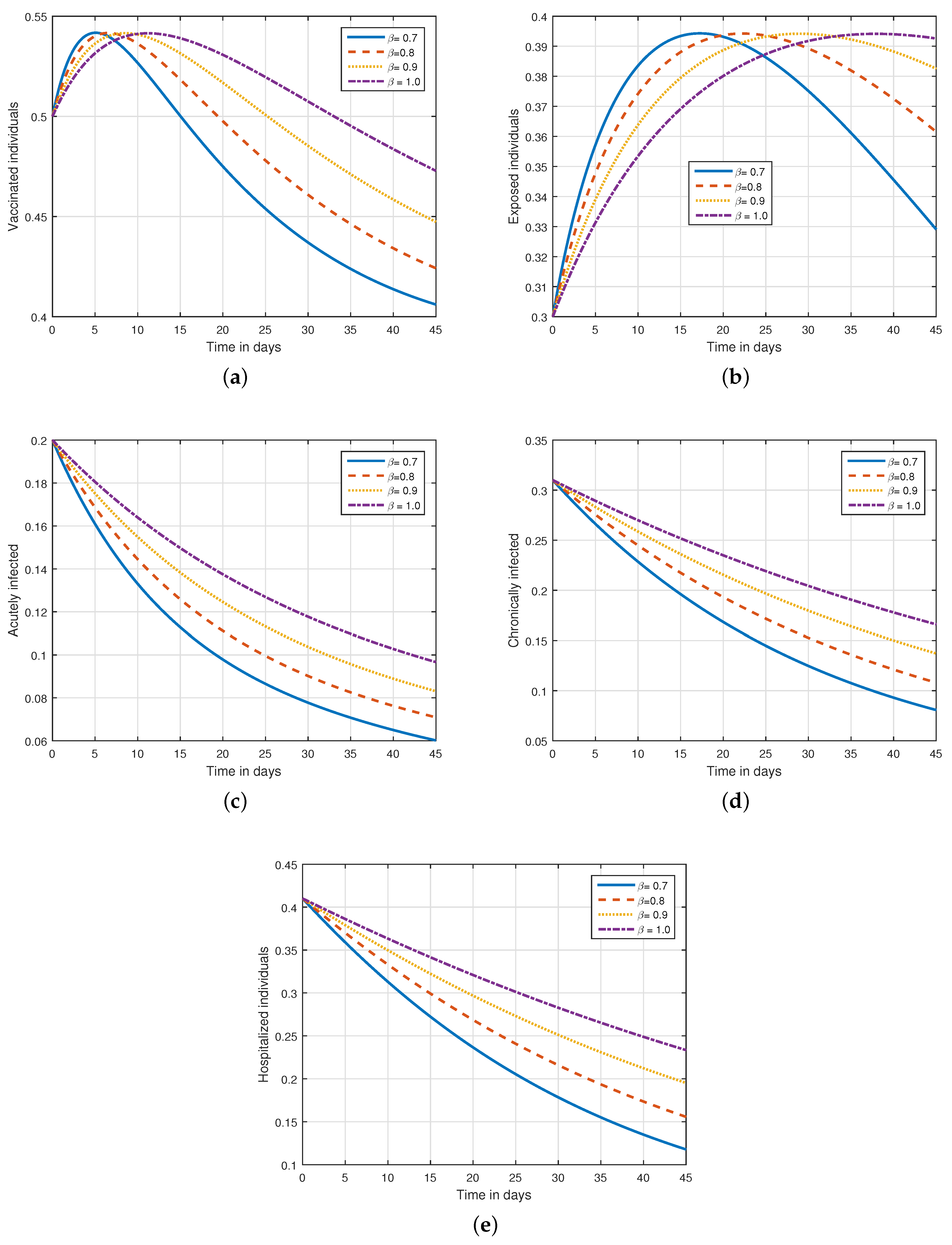
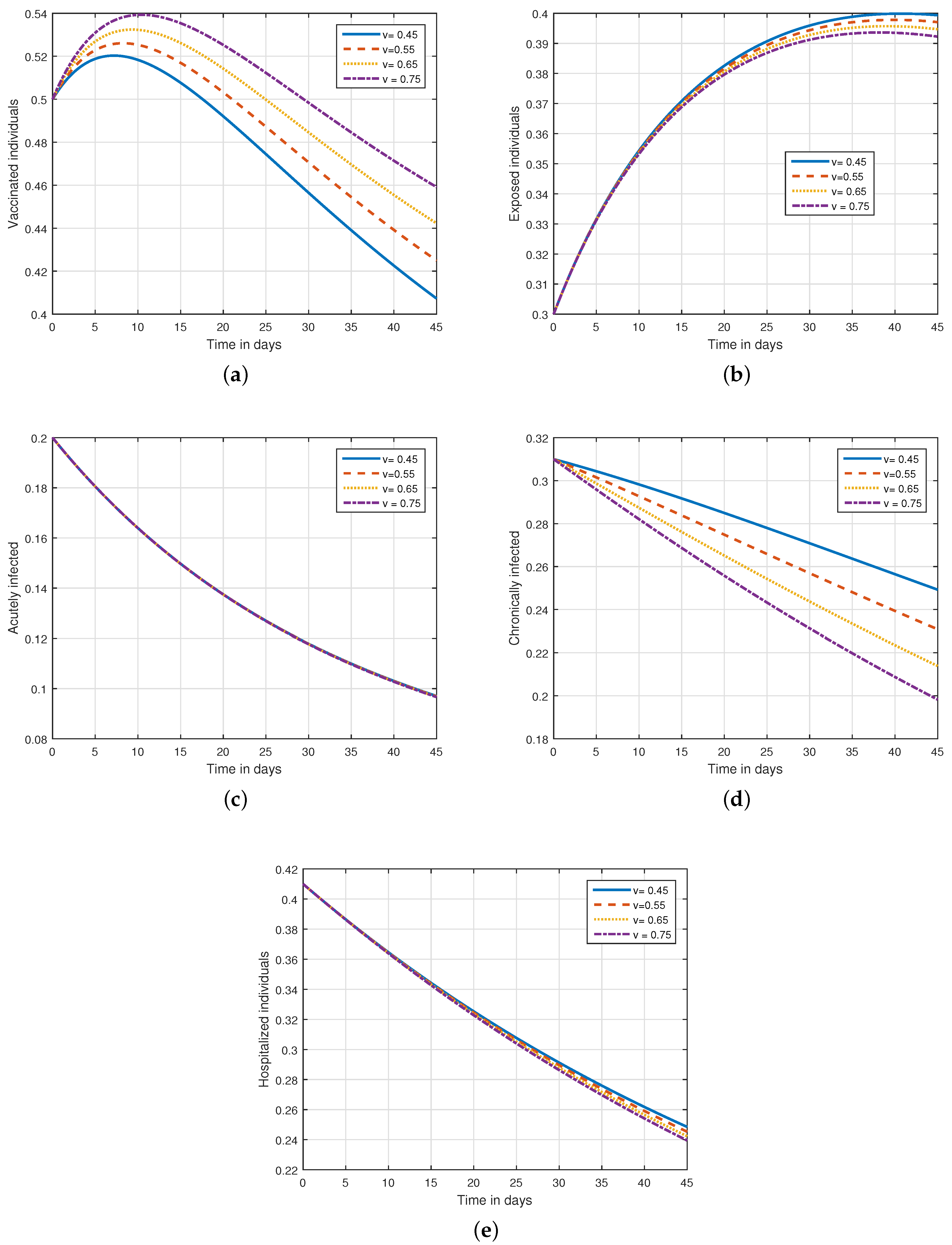
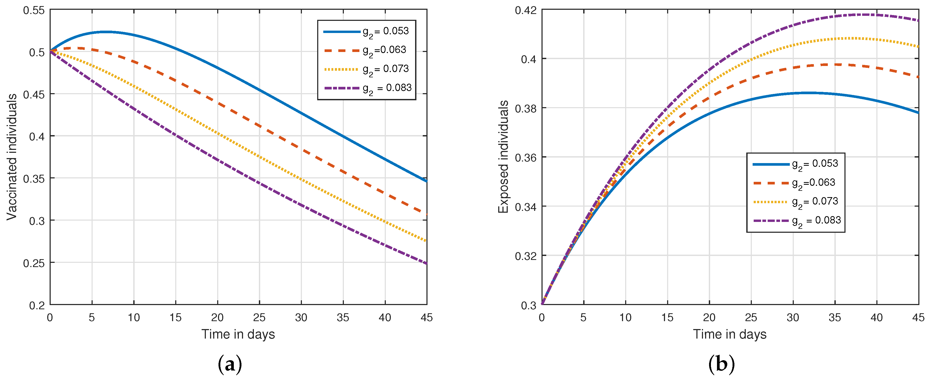
In Figure 1, we illustrate the impact of the fractional parameter on the solution pathways of the system of HBV infection to check whether this parameter of the system can be used as a preventive measure or not. The values of are chosen to be , and in the first simulation. It can be seen that the infection level can be decreased by decreasing the value of the input parameter . We noticed that this input factor contributes significantly and can be used as a control parameter, therefore, suggested this to the policymakers. In Figure 1, a comparative analysis of integer and non-integer derivatives are also illustrated. The curve for represents the integer case, while curves with other values of demonstrate non-integer cases. The effect of vaccination on the dynamics of HBV infection is shown in Figure 2. In this simulation, we assumed different values of the vaccination factor v, i.e., , and . We observed that an increase in v decreases the exposed and chronically infected individuals of the system. We recommended increasing the efficiency of vaccination for better control of the disease. In Figure 3, the effect of the loss rate of immunity due to vaccination is illustrated on the vaccinated and exposed individuals of the system. It can be seen that this factor is dangerous and can increase the risk of infection in society.
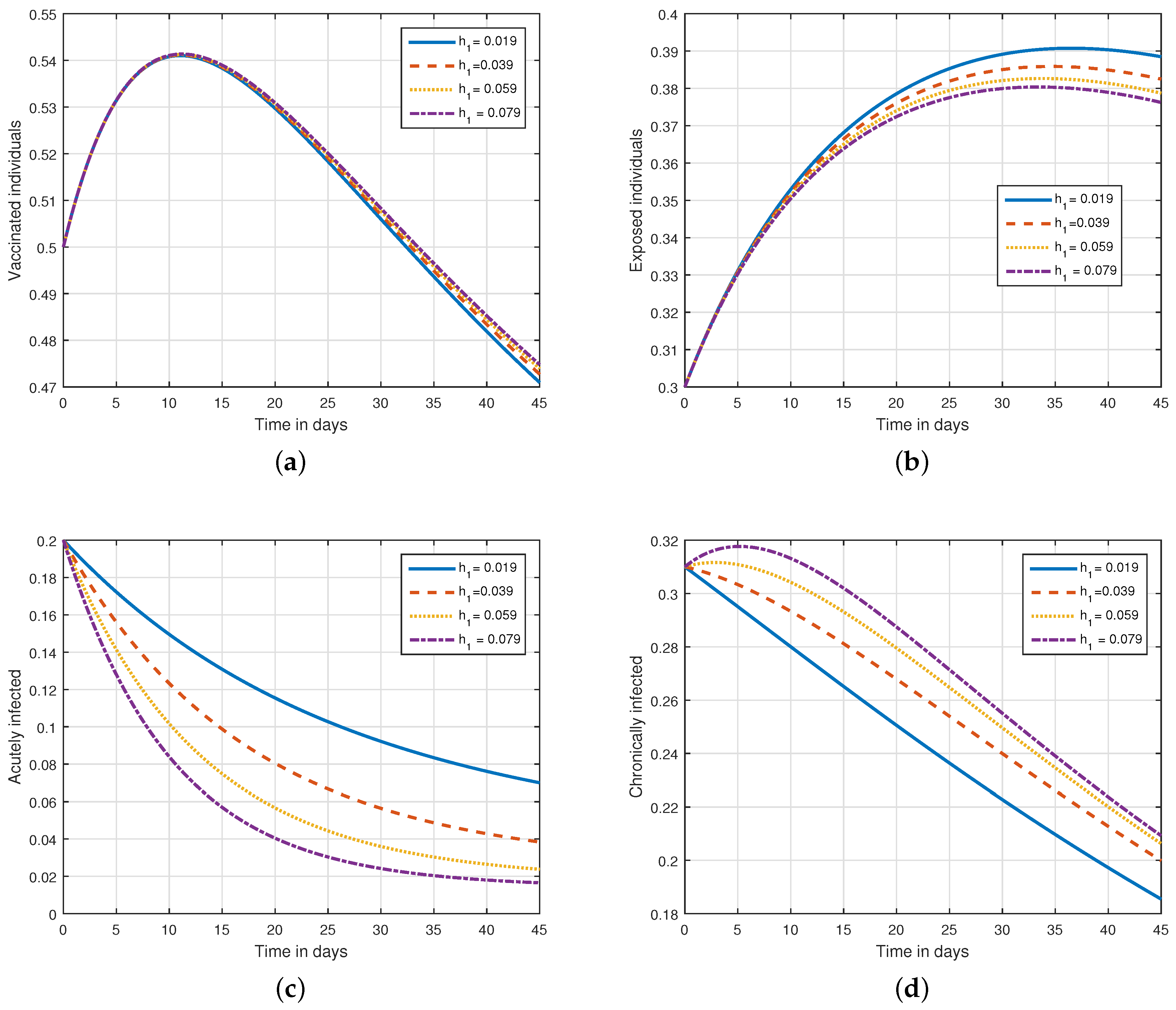
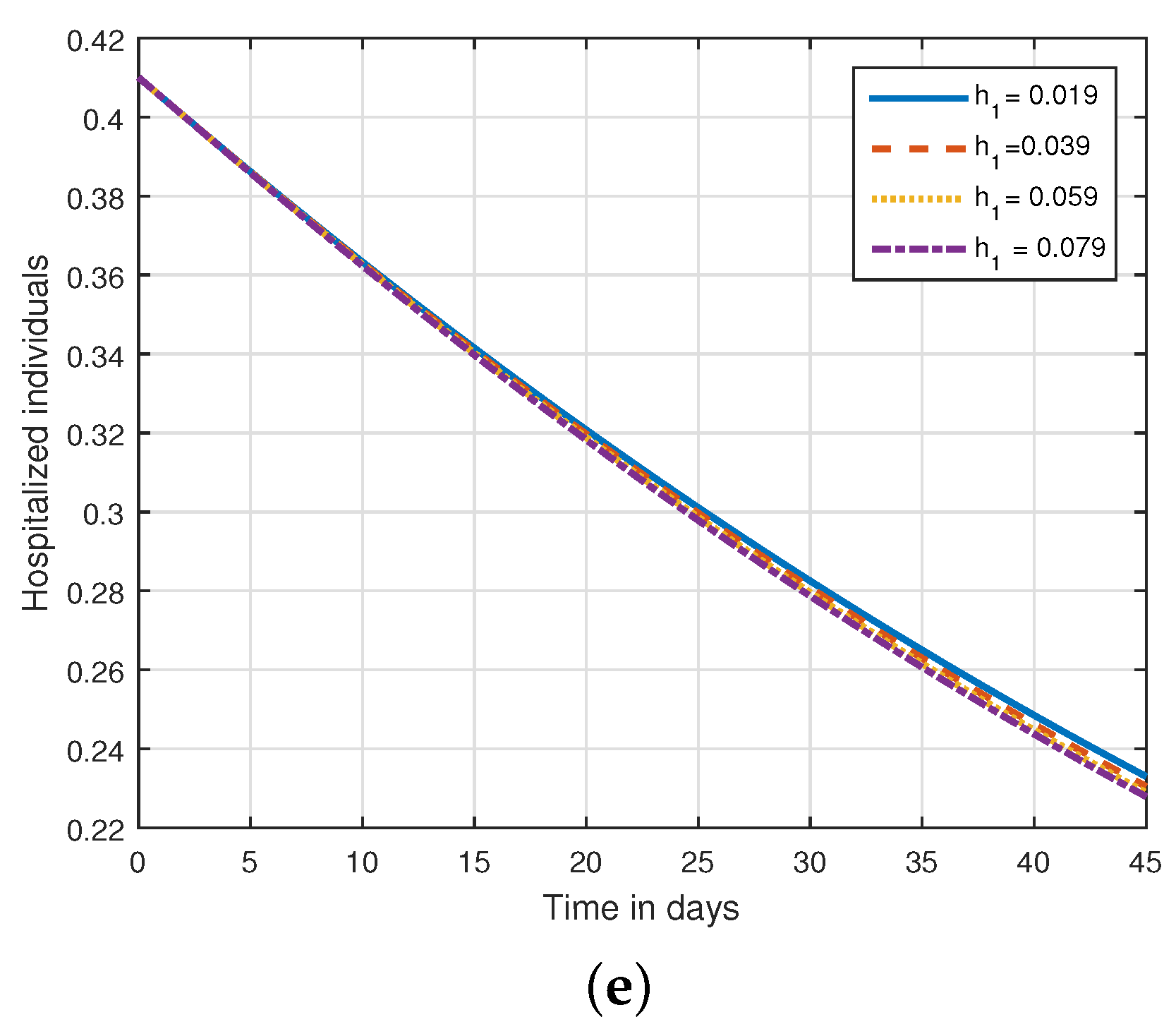
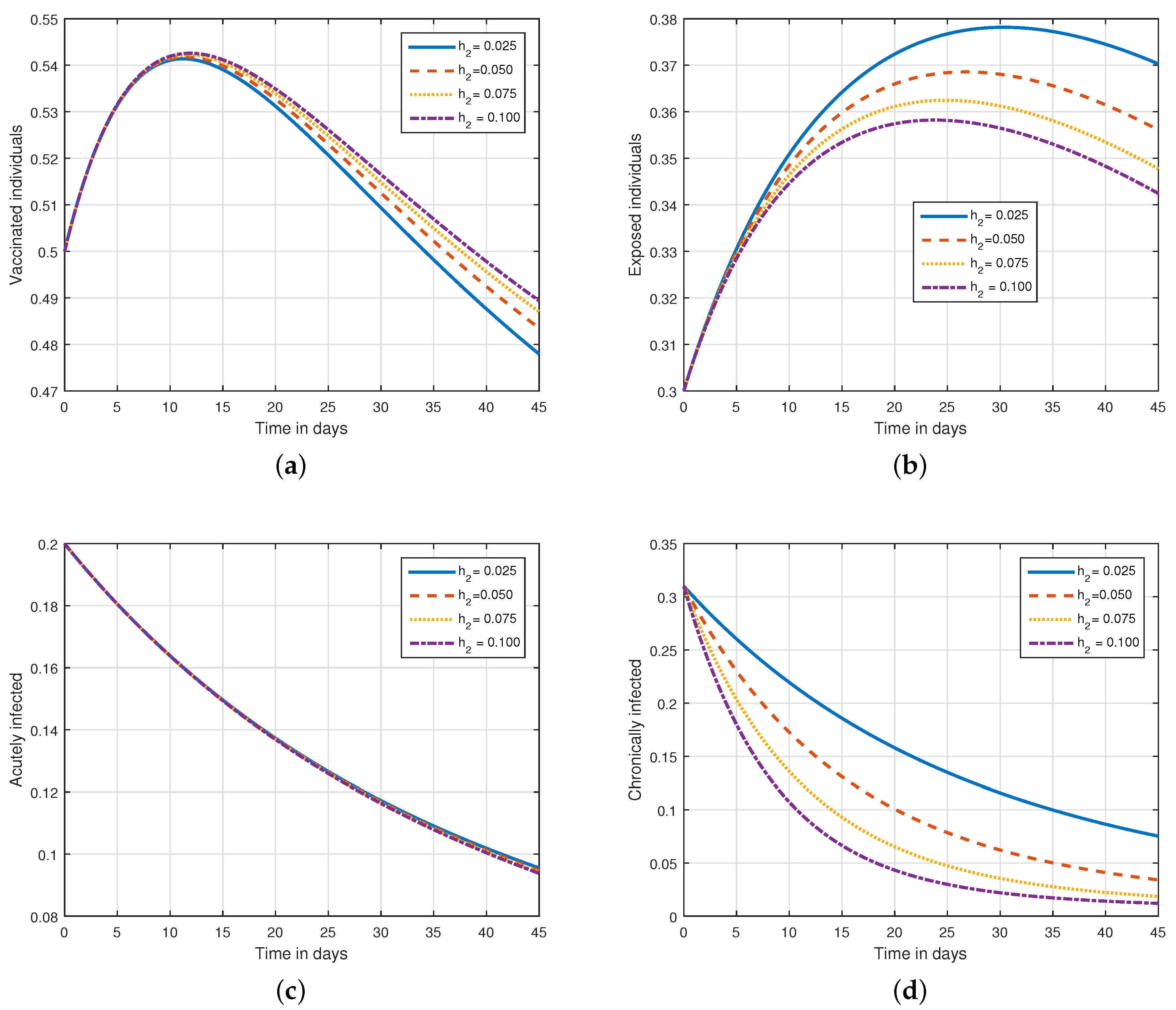
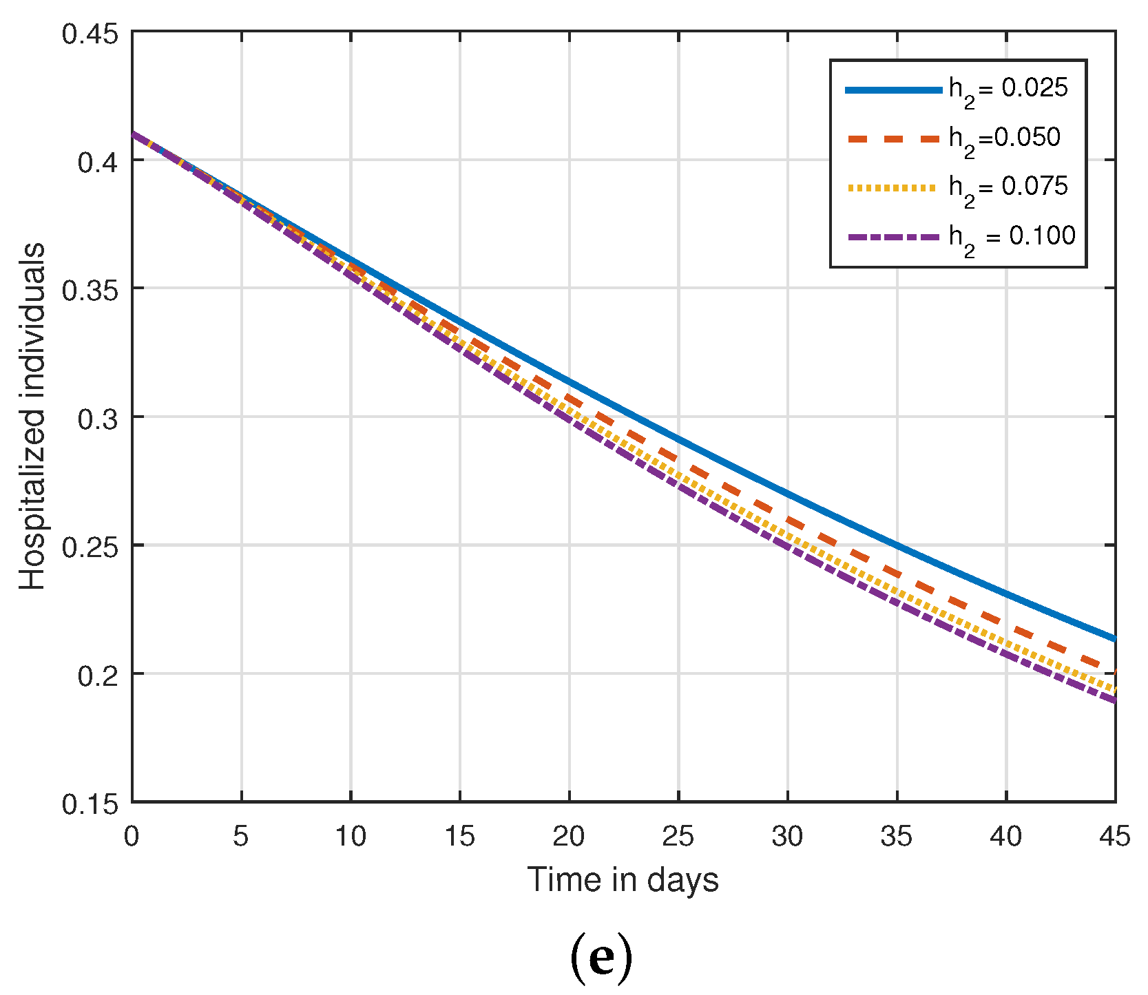
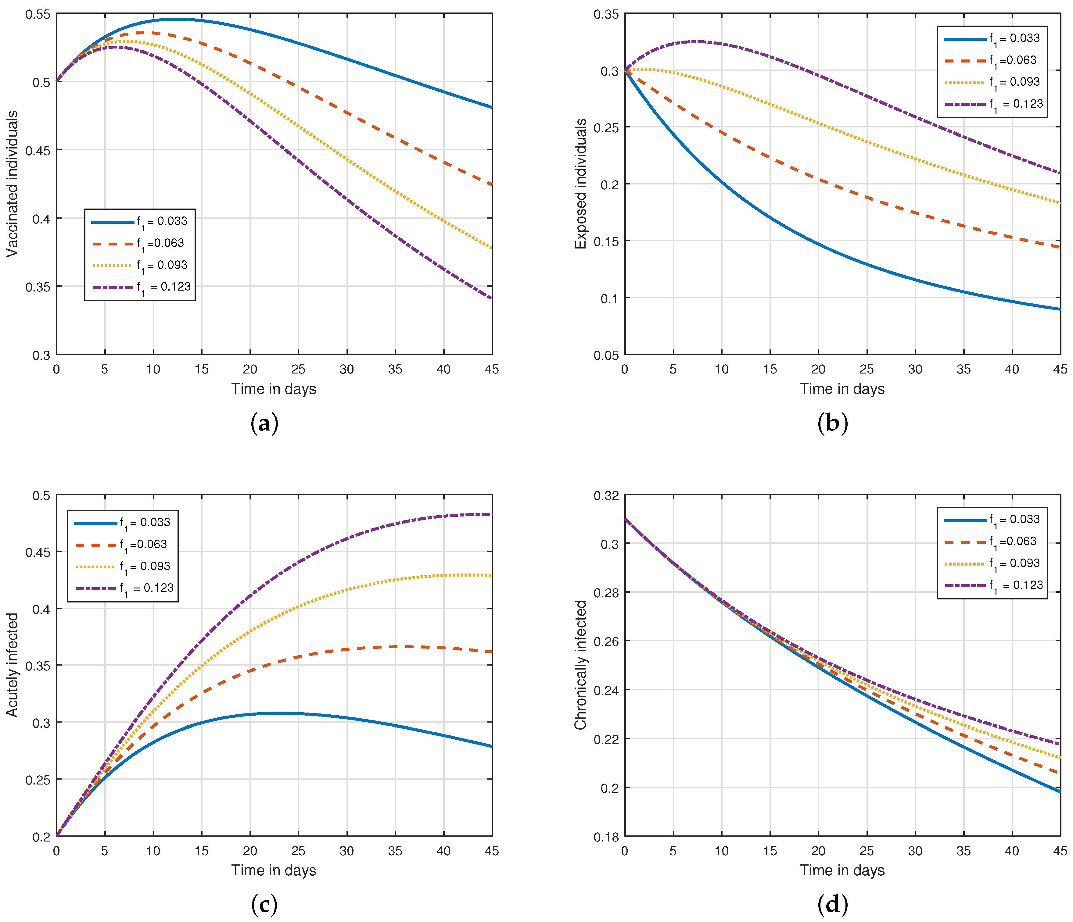
To visualize the impact of and on the system, we performed two different simulations, shown in Figure 4 and Figure 5. In Figure 4, we take , and while the values of are assumed to be , and in FigureFigure 5. It is clear from the figures how the infected individuals behave with the variation of these parameters. In the final simulation, presented in Figure 6, the solution pathways of the system are highlighted with the variation in transmission rate . In Figure 6, we assumed the values of to be , , , and to identify the role of on the dynamics of HBV infection. We noticed that this parameter is critical and highly increases the endemic level of the infection in society. This implies that the transmission rate is sensitive and needs to be controlled.
It is evident that HBV is a dangerous infectious disease, therefore, effective interventions are needed to eradicate and eliminate this viral infection from society. The control of the transmission rate and fractional parameter will reduce the intensity of the infection. Therefore, the control of these factors is recommended to officials. We also suggest increasing the efficiency of vaccination and medication through hospitalization for better prevention of the infection.
7. Conclusions
In this work, we constructed an epidemic model for HBV infection with vaccination and medication through hospitalization. The model is structured in a fractional framework for more accurate outcomes. We examined the steady states and determined the threshold parameter, indicated by . The stability result of the infection-free steady state was established. The existence and uniqueness of the hypothesized system’s solution are investigated using the fixed-point theorem in the context of Banach’s and Schaefer’s theorems. In our HBV system, we established the essential conditions for Ulam–Hyers stability. A time-series analysis of the system is presented through a numerical method. We have shown the impact of different parameters on the solution pathways of the system and recommended the most critical scenario of the system for the prevention and control of the infection. This model can assist in saving lives and prevent the spread of the infection by offering valuable information on the transmission dynamics of HBV and the efficacy of diverse intervention strategies. HBV infection is often associated with other comorbidities, such as HIV, hepatitis C, and liver cancer. These comorbidities can affect the course of HBV infection and complicate the design of effective control strategies. In future work, we will explore how comorbidities interact with HBV infection and how they can be incorporated into the model to better understand the overall disease burden and design more effective interventions.
Author Contributions
Conceptualization, S.A. and R.J.; Methodology, S.A.; Software, R.J.; Validation, R.J.; Investigation, S.A.; Resources, S.A.; Writing—original draft, S.A. and R.J.; Visualization, R.J. All authors have read and agreed to the published version of the manuscript.
Funding
This research received no external funding.
Institutional Review Board Statement
Not applicable.
Informed Consent Statement
Not applicable.
Data Availability Statement
Not applicable.
Acknowledgments
This research work was funded by Institutional Fund Projects under grant no. IFPIP: 1275-662-1443. The authors gratefully acknowledge technical and financial support provided by the Ministry of Education and King Abdulaziz University, DSR, Jeddah, Saudi Arabia.
Conflicts of Interest
The authors declare no conflict of interest.
References
- Pierce-Williams, R.A.; Sheffield, J.S. Hepatitis B in the Perinatal Period. In Neonatal Infections: Pathophysiology, Diagnosis, and Management; Springer: Cham, Switzerland, 2018; pp. 103–109. [Google Scholar]
- Zheng, Y.; Wu, J.; Ding, C.; Xu, K.; Yang, S.; Li, L. Disease burden of chronic hepatitis B and complications in China from 2006 to 2050: An individual-based modeling study. Virol. J. 2020, 17, 1–10. [Google Scholar] [CrossRef] [PubMed]
- Pang, J.; Cui, J.A.; Zhou, X. Dynamical behavior of a hepatitis B virus transmission model with vaccination. J. Theor. Biol. 2010, 265, 572–578. [Google Scholar] [CrossRef]
- Medley, G.F.; Lindop, N.A.; Edmunds, W.J.; Nokes, D.J. Hepatitis-B virus endemicity: Heterogeneity, catastrophic dynamics and control. Nat. Med. 2001, 7, 619–624. [Google Scholar] [CrossRef] [PubMed]
- Thornley, S.; Bullen, C.; Roberts, M. Hepatitis B in a high prevalence New Zealand population: A mathematical model applied to infection control policy. J. Theor. Biol. 2008, 254, 599–603. [Google Scholar] [CrossRef] [PubMed]
- Zou, L.; Zhang, W.; Ruan, S. Modeling the transmission dynamics and control of hepatitis B virus in China. J. Theor. Biol. 2010, 262, 330–338. [Google Scholar] [CrossRef]
- Pang, J.; Cui, J.A.; Hui, J. The importance of immune responses in a model of hepatitis B virus. Nonlinear Dyn. 2012, 67, 723–734. [Google Scholar] [CrossRef]
- Wang, K.; Wang, W.; Song, S. Dynamics of an HBV model with diffusion and delay. J. Theor. Biol. 2008, 253, 36–44. [Google Scholar] [CrossRef]
- Xu, R.; Ma, Z. An HBV model with diffusion and time delay. J. Theor. Biol. 2009, 257, 499–509. [Google Scholar] [CrossRef]
- Zhao, S.; Xu, Z.; Lu, Y. A mathematical model of hepatitis B virus transmission and its application for vaccination strategy in China. Int. J. Epidemiol. 2000, 29, 744–752. [Google Scholar] [CrossRef]
- Khan, M.A.; Islam, S.; Arif, M. Transmission model of hepatitis B virus with the migration effect. Biomed Res. Int. 2013, 2013. [Google Scholar] [CrossRef]
- Zhang, T.; Wang, K.; Zhang, X. Modeling and analyzing the transmission dynamics of HBV epidemic in Xinjiang, China. PLoS ONE 2015, 10, e0138765. [Google Scholar] [CrossRef] [PubMed]
- Khan, M.A.; Islam, S.; Zaman, G. Media coverage campaign in Hepatitis B transmission model. Appl. Math. Comput. 2018, 331, 378–393. [Google Scholar] [CrossRef]
- Alrabaiah, H.; Safi, M.A.; DarAssi, M.H.; Al-Hdaibat, B.; Ullah, S.; Khan, M.A.; Shah, S.A.A. Optimal control analysis of hepatitis B virus with treatment and vaccination. Results Phys. 2020, 19, 103599. [Google Scholar] [CrossRef]
- Sowndarrajan, P.T.; Shangerganesh, L.; Debbouche, A.; Torres, D.F. Optimal control of a heroin epidemic mathematical model. Optimization 2022, 71, 3107–3131. [Google Scholar] [CrossRef]
- Sun, H.; Zhang, Y.; Baleanu, D.; Chen, W.; Chen, Y. A new collection of real world applications of fractional calculus in science and engineering. Commun. Nonlinear Sci. Numer. Simul. 2018, 64, 213–231. [Google Scholar] [CrossRef]
- Opoku, M.O.; Wiah, E.N.; Okyere, E.; Sackitey, A.L.; Essel, E.K.; Moore, S.E. Stability Analysis of Caputo Fractional Order Viral Dynamics of Hepatitis B Cellular Infection. Math. Comput. Appl. 2023, 28, 24. [Google Scholar] [CrossRef]
- Samraiz, M.; Perveen, Z.; Abdeljawad, T.; Iqbal, S.; Naheed, S. On certain fractional calculus operators and applications in mathematical physics. Phys. Scr. 2020, 95, 115210. [Google Scholar] [CrossRef]
- Jan, R.; Boulaaras, S. Analysis of fractional-order dynamics of dengue infection with non-linear incidence functions. Trans. Inst. Meas. Control 2022, 44, 2630–2641. [Google Scholar] [CrossRef]
- Tang, T.Q.; Shah, Z.; Jan, R.; Deebani, W.; Shutaywi, M. A robust study to conceptualize the interactions of CD4+ T-cells and human immunodeficiency virus via fractional-calculus. Phys. Scr. 2021, 96, 125231. [Google Scholar] [CrossRef]
- Kilbas, A.A.; Srivastava, H.M.; Trujillo, J.J. Theory and Applications of Fractional Differential Equations; Elsevier: Amsterdam, The Netherlands, 2006; Volume 204. [Google Scholar]
- Podlubny, I. Fractional Differential Equations: An Introduction to Fractional Derivatives, Fractional Differential Equations, to Methods of Their Solution and Some of Their Applications; Elsevier: Amsterdam, The Netherlands, 1998. [Google Scholar]
- Granas, A.; Dugundji, J. Elementary fixed point theorems. In Fixed Point Theory; Springer: New York, NY, USA, 2003; pp. 9–84. [Google Scholar]
- Van den Driessche, P.; Watmough, J. Reproduction numbers and sub-threshold endemic equilibria for compartmental models of disease transmission. Math. Biosci. 2002, 180, 29–48. [Google Scholar] [CrossRef]
- Martcheva, M. An Introduction to Mathematical Epidemiology; Springer: New York, NY, USA, 2015; Volume 61, pp. 9–31. [Google Scholar]
- Ullam, S.M. Problems in Modern Mathematics (Chapter VI); Wiley: New York, NY, USA, 1940. [Google Scholar]
- Hyers, D.H. On the stability of the linear functional equation. Proc. Natl. Acad. Sci. USA 1941, 27, 222. [Google Scholar] [CrossRef]
- Rassias, T.M. On the stability of the linear mapping in Banach spaces. Proc. Am. Math. Soc. 1978, 72, 297–300. [Google Scholar] [CrossRef]
- Benkerrouche, A.; Souid, M.S.; Etemad, S.; Hakem, A.; Agarwal, P.; Rezapour, S.; Ntouyas, S.K.; Tariboon, J. Qualitative Study on Solutions of a Hadamard Variable Order Boundary Problem via the Ulam-Hyers-Rassias Stability. Fractal Fract. 2021, 5, 108. [Google Scholar] [CrossRef]
- Atangana, A.; Owolabi, K.M. New numerical approach for fractional differential equations. Math. Model. Nat. Phenom. 2018, 13, 3. [Google Scholar] [CrossRef]
Figure 1.
Illustration of the solution pathways of (a) vaccinated individuals, (b) exposed individuals, (c) acutely infected, (d) chronically infected and (e) hospitalized individuals of the recommended system (6) of HBV infection with different values of , i.e., .
Figure 1.
Illustration of the solution pathways of (a) vaccinated individuals, (b) exposed individuals, (c) acutely infected, (d) chronically infected and (e) hospitalized individuals of the recommended system (6) of HBV infection with different values of , i.e., .

Figure 2.
Illustration of the solution pathways of (a) vaccinated individuals, (b) exposed individuals, (c) acutely infected, (d) chronically infected and (e) hospitalized individuals of the recommended system (6) of HBV infection with different values of v, i.e., .
Figure 2.
Illustration of the solution pathways of (a) vaccinated individuals, (b) exposed individuals, (c) acutely infected, (d) chronically infected and (e) hospitalized individuals of the recommended system (6) of HBV infection with different values of v, i.e., .

Figure 3.
Time series analysis of (a) vaccinated individuals and (b) exposed individuals of the recommended system (6) of HBV infection with different values of the input parameter , i.e., .
Figure 3.
Time series analysis of (a) vaccinated individuals and (b) exposed individuals of the recommended system (6) of HBV infection with different values of the input parameter , i.e., .

Figure 4.
Time-series analysis of (a) vaccinated individuals, (b) exposed individuals, (c) acutely infected, (d) chronically infected and (e) hospitalized individuals of the recommended system (6) of HBV infection with different values of the input parameter , i.e., .
Figure 4.
Time-series analysis of (a) vaccinated individuals, (b) exposed individuals, (c) acutely infected, (d) chronically infected and (e) hospitalized individuals of the recommended system (6) of HBV infection with different values of the input parameter , i.e., .


Figure 5.
Graphical view analysis of (a) vaccinated individuals, (b) exposed individuals, (c) acutely infected, (d) chronically infected and (e) hospitalized individuals of the recommended system (6) of HBV infection with different values of the input parameter , i.e., .
Figure 5.
Graphical view analysis of (a) vaccinated individuals, (b) exposed individuals, (c) acutely infected, (d) chronically infected and (e) hospitalized individuals of the recommended system (6) of HBV infection with different values of the input parameter , i.e., .


Figure 6.
Representation of the solution pathways of (a) vaccinated individuals, (b) exposed individuals, (c) acutely infected, (d) chronically infected and (e) hospitalized individuals of the recommended system (6) of HBV infection with different values of the input parameter , i.e., .
Figure 6.
Representation of the solution pathways of (a) vaccinated individuals, (b) exposed individuals, (c) acutely infected, (d) chronically infected and (e) hospitalized individuals of the recommended system (6) of HBV infection with different values of the input parameter , i.e., .


Disclaimer/Publisher’s Note: The statements, opinions and data contained in all publications are solely those of the individual author(s) and contributor(s) and not of MDPI and/or the editor(s). MDPI and/or the editor(s) disclaim responsibility for any injury to people or property resulting from any ideas, methods, instructions or products referred to in the content. |
© 2023 by the authors. Licensee MDPI, Basel, Switzerland. This article is an open access article distributed under the terms and conditions of the Creative Commons Attribution (CC BY) license (https://creativecommons.org/licenses/by/4.0/).
Share and Cite
MDPI and ACS Style
Alyobi, S.; Jan, R. Qualitative and Quantitative Analysis of Fractional Dynamics of Infectious Diseases with Control Measures. Fractal Fract. 2023, 7, 400. https://doi.org/10.3390/fractalfract7050400
AMA Style
Alyobi S, Jan R. Qualitative and Quantitative Analysis of Fractional Dynamics of Infectious Diseases with Control Measures. Fractal and Fractional. 2023; 7(5):400. https://doi.org/10.3390/fractalfract7050400
Chicago/Turabian StyleAlyobi, Sultan, and Rashid Jan. 2023. "Qualitative and Quantitative Analysis of Fractional Dynamics of Infectious Diseases with Control Measures" Fractal and Fractional 7, no. 5: 400. https://doi.org/10.3390/fractalfract7050400