
Depth Image Enhancement Algorithm Based on Fractional Differentiation


1
School of Electronic and Information Engineering, Changchun University of Science and Technology, Changchun 130022, China
2
Xi’an Key Laboratory of Active Photoelectric Imaging Detection Technology, Xi’an Technological University, Xi’an 710021, China
*
Authors to whom correspondence should be addressed.
Fractal Fract. 2023, 7(5), 394; https://doi.org/10.3390/fractalfract7050394
Submission received: 31 March 2023
/
Revised: 29 April 2023
/
Accepted: 10 May 2023
/
Published: 11 May 2023
(This article belongs to the Special Issue Fractional Order Complex Systems: Advanced Control, Intelligent Estimation and Reinforcement Learning Image Processing Algorithms)
Abstract
:Depth image enhancement techniques can help to improve image quality and facilitate computer vision tasks. Traditional image-enhancement methods, which are typically based on integer-order calculus, cannot exploit the textural information of an image, and their enhancement effect is limited. To solve this problem, fractional differentiation has been introduced as an innovative image-processing tool. It enables the flexible use of local and non-local information by taking into account the continuous changes between orders, thereby improving the enhancement effect. In this study, a fractional differential is applied in depth image enhancement and used to establish a novel algorithm, named the fractional differential-inverse-distance-weighted depth image enhancement method. Experiments are performed to verify the effectiveness and universality of the algorithm, revealing that it can effectively solve edge and hole interference and significantly enhance textural details. The effects of the order of fractional differentiation and number of iterations on the enhancement performance are examined, and the optimal parameters are obtained. The process data of depth image enhancement associated with the optimal number of iterations and fractional order are expected to facilitate depth image enhancement in actual scenarios.
1. Introduction
In recent years, with the growing popularity of artificial intelligence and autonomous driving technologies, depth image processing algorithms have attracted increasing attention. A depth image is an image that contains depth information in each pixel, which can be used in three-dimensional (3D) reconstruction, object detection, face recognition, and in other fields. Depth image processing involves several problems, such as low contrast, high noise, and blurring problems. To address the problem of insufficient textural information in a depth image, mainstream processing methods focus on enhancing the edge of a depth image. However, only a few methods can effectively enhance the textural information of depth images without introducing fuzzy information. Consequently, depth image enhancement is a research hotspot at present, especially as enhancing the texture of a depth image can enable the obtainment of additional textural information from an image.
Various depth image processing algorithms have been developed. Masahiro devised a method to reduce the noise and number of voids in a depth image pixel by pixel and thereby improve the resolution [1]. Specifically, by reducing the depth image random noise, the coordinates of the correct object surface are obtained; missing values are thus identified and then inserted between the existing pixels. Subsequently, new pixels are inserted between them to enhance the depth image. Zhang et al. developed an image enhancement algorithm based on an adaptive median filter and fractional-order differential [2]. Wang et al. devised an image-denoising method based on fractional quaternion wavelet analysis [3]. Zhou et al. used the fractal dimension method to enhance a depth image [4]. Moreover, Zhou et al. established an edge-guided method for the super-resolution of depth images to obtain high-quality edge information. The edge-guided method can maintain edge sharpness, thereby avoiding blurry and jagged edges during depth image processing [5]. Researchers have also used a variety of image processing techniques, such as histogram matching, edge-preserving filtering, and local contrast enhancement, to improve the quality and clarity of depth images [6,7,8].
The above-described studies have provided strong support and useful references for depth image processing. However, the existing algorithms have several limitations, such as high complexity, low processing efficiency, and an inability to adapt to different scenarios. Thus, there is a need for efficient, stable, and reliable algorithms capable of depth image enhancement. Fractional differentiation is an emerging differential method that has wider applicability and stronger expressive power than existing methods. Moreover, fractional differentiation has been widely applied in the field of image processing with promising results. Fractional calculus is a mathematical tool that extends traditional integer-order calculus to non-integer orders and can be used to analyse complex systems with long memory and non-local dependencies. By incorporating fractional calculus into image processing techniques, researchers have improved these techniques’ image enhancement, restoration, and segmentation performances.
For example, Gupta et al. devised an adaptive image-denoising algorithm based on generalised fractional integration and fractional differentiation [9]. They combined this algorithm with an innovative noise-detection method to detect salt-and-pepper noise in images. Moreover, they used an adaptive mask based on generalised fractional integration to update noise-free pixels to enhance the details of images. This framework served as a flexible tool for image enhancement and image denoising. Zhang et al. designed an image fusion method based on fractional difference, which enables better visual perception and more objective evaluation and retains more image details than traditional methods [10]. Harjule et al. compared the traditional method with a fractional-order-based method for texture enhancement in medical images. To minimise the mean square error, the fractional-order operator for all images was optimised using the grey wolf optimiser. The results indicated that score-based operators with a differential order outperformed traditional integer order operators in the textural enhancement of medical images [11]. Zhang constructed a new image-enhancement algorithm based on a rough set and a fractional-order differentiator. An image enhanced by this algorithm has a clear edge and rich textural details, and it can retain information from the smooth areas in an image [12,13].
Despite these promising results, several limitations remain to be addressed. First, most existing methods consider only the local features of images and ignore the non-local dependencies between different regions. Second, these methods may not be effective for images containing complex textures or structures. Finally, only a few researchers have focused on depth image enhancement processing and the application of fractional differentials in depth image processing. Therefore, the introduction of fractional calculus in depth image applications must be further explored.
This study aims to apply a fractional differential for depth image enhancement. This application involves several challenges, such as avoiding the introduction of fuzzy information and inconsistency with an actual scene. To address these problems, an improved algorithm, named the fractional differential-inverse-distance-weighted depth image enhancement method, is developed. The results of experiments show that the algorithm can effectively integrate local and non-local information into the enhancement process and effectively enhance depth images with complex textures and structures.
The remainder of this paper is organised as follows. Section 2 describes the application of a fractional differential in image enhancement and the result, and discusses the problems in a depth image subjected to fractional differential enhancement. Section 3 describes the inverse distance weighting technique and the development of the fractional differential-inverse-distance-weighting depth image enhancement method. The method is used to enhance depth images of different orders, and the fractional differential order is optimised. The results indicate that the algorithm is effective. Section 4 presents the experimental results. The algorithm is applied to the depth image of a dataset, and the effect of the fractional differential small order and number of iterations on the algorithm’s performance is verified. The results show that the algorithm is universal, can effectively solve the interference of edges and voids in depth images, and can enhance textural details. Section 5 presents the concluding remarks and recommendations for future research.
2. Fractional-Differential-Based Depth Image Enhancement
As an important branch of digital image processing, image enhancement has broad application aspects. The visual effect of image shooting may not be satisfactory owing to environmental conditions, and thus, image enhancement methods must be used (i.e., certain features of the target object in an image must be improved). Acquiring the typical characteristic parameters of a target in an image enables the effective recognition and detection of the target in the image [14,15]. The objective of image enhancement processing is to strengthen the valuable areas in an image and weaken or remove the non-essential information in the image. By enhancing the useful information, the image obtained in an actual scene can be transformed into an image that can be analysed and processed by humans or other systems. The features of an image (that is, the main information contained in the image) are typically present in the edge and textural details. Enhancing textural feature information can provide a valuable basis for further processing, such as image segmentation, recognition, or super-resolution. Fractional differentiation can help to improve the high-frequency and instantaneous-frequency (IF) parts of a signal, thereby nonlinearly strengthening the IF component while preserving the low-frequency and direct current parts. That is, fractional differentiation can enhance the edge and contour information and weak textural areas of an image. Thus, fractional differentiation is a valuable tool in image processing [16,17,18,19,20].
According to fractional calculus theory, a fractional differential operator has a weak reciprocal, which can enhance the high-frequency components of a signal while retaining the low-frequency components [21]. Therefore, by applying fractional calculus theory to image processing, the prominence of the edges of an image can be increased while retaining the textural information of the smooth areas of the image. It is generally believed that the value of fractional calculus theory and algorithms in image processing lies in their ability to add an additional degree of freedom. By selecting the appropriate fractional order and constructing a convolutional mask operator to select the fractional order satisfactory results for image signal enhancement and image signal denoising can be achieved. Guo et al. derived the formula of a fractional differential operator, realised the enhancement of a two-dimensional (2D) image based on the Grumwald–Letnikov (G–L) definition and a fractional calculus model, and discussed its application in image processing [21,22,23].
2.1. Construction Based on a Fractional Differential Operator
Based on the G–L definition, a v-order differential can be expressed as follows (Equation (1)):
where is the fractional differential order; is the calculus step size; a and t are the lower and upper bounds for fractional calculus, respectively; is the gamma function; is the binomial coefficient.
The continuous interval of the one-dimensional signal is defined as and divided equally into units specified by . Then, the equivalent expression of the v (v ≥ 0)-order fractional differential of the unary signal is
The 2D signal is defined by assuming that the fractional differential of for the two directions (x- and y-axes) are separable in certain conditions. Given the separability of the Fourier transform, it can be used to extend the fractional calculus from one-dimensional space to two-dimensional space. The 2D image signal is equally divided by (unit time) to realise the fractional differentiation of the x- and y-axes.
From the equivalent expression of Equation (3), the approximate solution of the fractional calculus of the x- and y-axes can be obtained as follows:
Using the limit form, the numerical expressions of the fractional differential in the x- and y-axis directions are as follows:
Equations (6) and (7) can be used to obtain the order fractional differential operator coefficient :
Assuming that the mask size is 3 × 3, i.e., if N = 3, the approximate solutions for the two axis directions can be obtained using Equations (7) and (8):
2.2. Fractional Differential Enhancement Operator and Convolution Template
By extending the formula of fractional differentiation to the other six directions, the approximate solutions of fractional differentiation in these six directions can be obtained. The eight directions are rotationally invariant; thus, the approximate solutions of fractional differentiation in these eight directions are used to construct the fractional differential operator.
Thus, the eight-directional mask template is established as shown in Figure 1. The coefficients for the positive and negative directions
of the x-axis are defined as and , respectively, with , , , and in the counterclockwise direction. The coefficients for the positive and negative directions of the y-axis are and , respectively.
The coefficients are defined as follows:
In an image, adjacent pixels have a certain similarity, and the closer the pixels are to the central target, the greater their similarity. Thus, the presence of too many adjacent pixels introduces unnecessary spatial and time complexities. Therefore, image processing should be aimed at exploiting the local neighbourhood pixel information of the target pixel. The 3 × 3 mask in eight directions is used to perform convolution calculations on the image point , which is 5 × 5 in size, as follows:
The convolution of each direction is calculated and weighted linearly to obtain the mask calculation results, as shown in Equation (15):
where
The image data are computed through the fractional differential mask convolution, and the convolution result is continuously enlarged or reduced. The results of convolution calculation can be normalised by defining the normalisation factor q as
Then, q is substituted into Equation (18), and a 5 × 5 mask template is used to obtain filtered data :
2.3. Effect of the Fractional Differential Enhancement Algorithm on the Depth Image
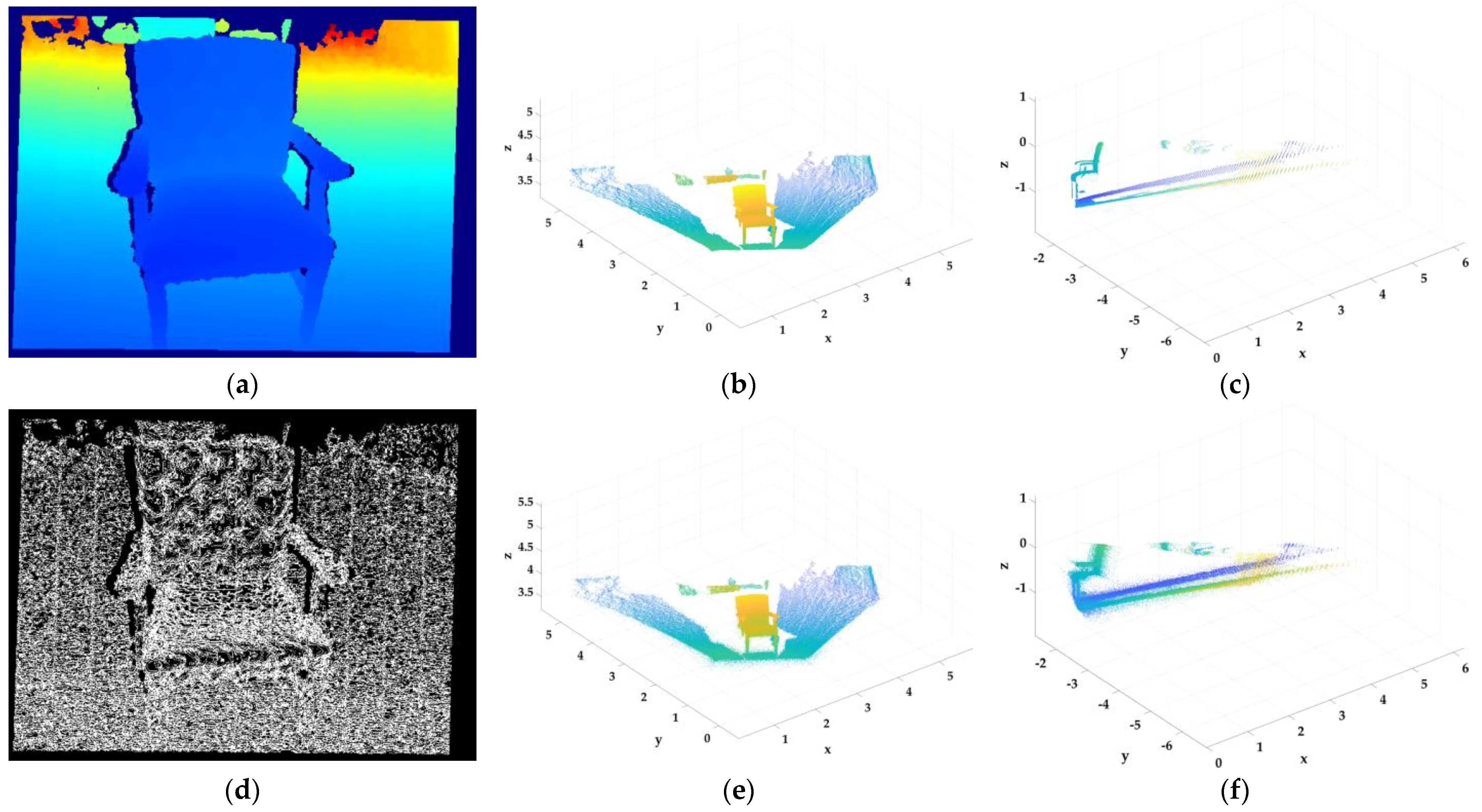
In a 2D image, noise and edges are discontinuities of the local features. The pixel values of noise and edges are considerably different from those of neighbouring areas. Thus, noise and edges correspond to high-frequency signals, which are enhanced by fractional differential pairs. Therefore, fractional differential filtering is performed on a depth image, and the filtered depth image and corresponding point cloud image are obtained.
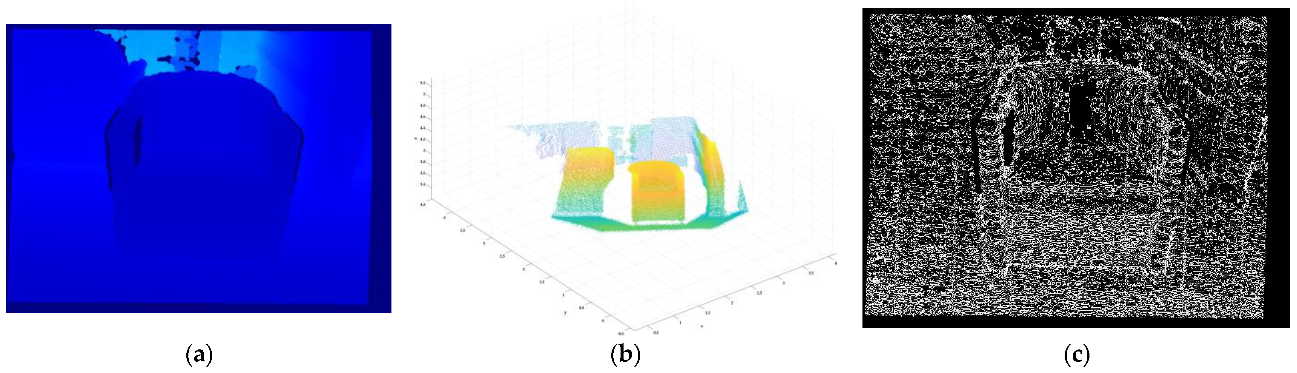
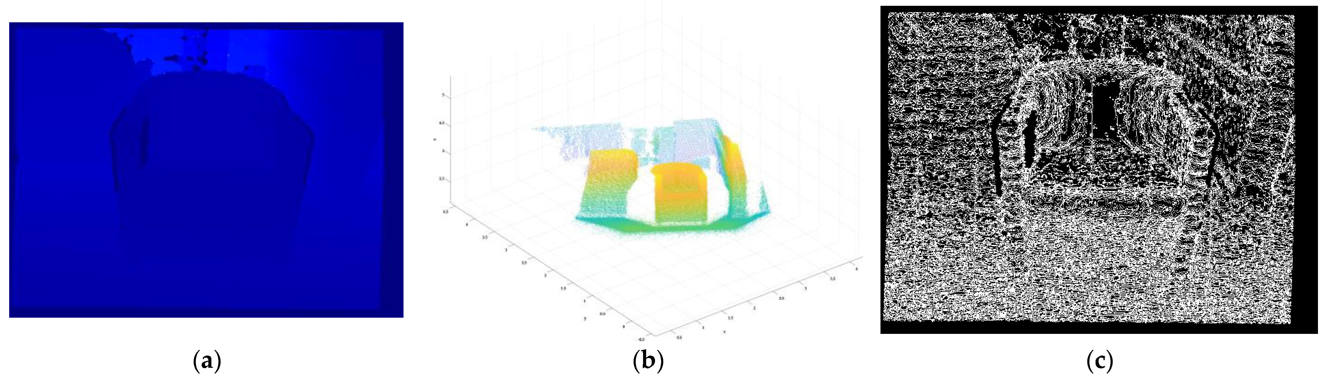
Figure 2 shows a depth image after fractional difference enhancement. The edge and noise points are enhanced to varying degrees. The point cloud image clearly shows the edges and several high-frequency noise spots. The objective of depth image enhancement is to enhance the textural information. However, as shown in Figure 2, edge noise is introduced into the depth image after fractional differential enhancement. Because the presence of such noise can limit the application of depth images in practical applications, such as 3D reconstruction, the enhancement method must be modified to effectively enhance the textural information.
As shown in Figure 2, the differential mask enhances high-frequency points or edge noise in the case of drastic changes in the edge information. However, the enhanced depth image cannot be used for 3D reconstruction. Moreover, according to experiments, gradient judgement-based methods cannot effectively distinguish weak noise from textural information.
3. Fractional differential-Inverse-Distance-Weighted Enhancement Algorithm
A depth image, also known as a range image, takes the distance (depth) from an image collector to each point in a scene as the pixel value, which directly reflects the geometric shape of the visible surface of the scene. Such images are also termed spatial distance images. Based on the principle of similarity, the depth value is used as a weight, and this is used to estimate a reasonable value for a point to be interpolated. Assuming that each adjacent point has a local influence, an inverse-distance-weighted model is constructed. The distance between the point to be interpolated and a sample point is used as the weighting factor for weighted summation. A sample point at a smaller distance corresponds to a higher weight, so the weight decreases as a function of the distance.
3.1. Design of the Fractional differential-Inverse-Distance-Weighting Algorithm
The point to be inserted into a space is defined as , and known scattered points exist in the neighbourhood of point . The attribute value of point is interpolated using the distance-weighted inverse ratio method. The inverse distance interpolation principle states that in calculating the attribute value of the point to be inserted, the attribute value of the known point in the neighbourhood of this point must be considered. The attribute value of the point to be inserted is obtained from the inverse distance weighted average. The weight is related to the distance between the point to be inserted and point in the neighbourhood, where is the power factor ( is generally set to 2).
where is defined as the unit of distance from the point to be inserted to the i-th point in its neighbourhood.
is defined as the distance from the point to be interpolated to the adjacent point , as follows:
The interpolation function represents the weighted average of the function value at each point, and is the function of the reciprocal of the interpolation, as follows:
The interpolation function is introduced into the data weighting process after fractional filtering, and the equalisation parameter φ is introduced considering that the function value may be zero.
Overall, is the depth value of the image point to be filtered, is one of the convolution sums of eight fractional operators, and is the new depth value after filtering.
The weighting calculation formula is modified, and the linear weighting formula presented in Equation (19) is used—based on the inverse distance weighting method—to derive a new inverse distance weighting formula, as follows:
Q, obtained using Equation (17), is added into Equation (27), and the new is obtained after applying the ν-order fractional differential filter with a 3 × 3 mask, as follows:
3.2. Depth Image Enhancement Effect of the Improved Algorithm
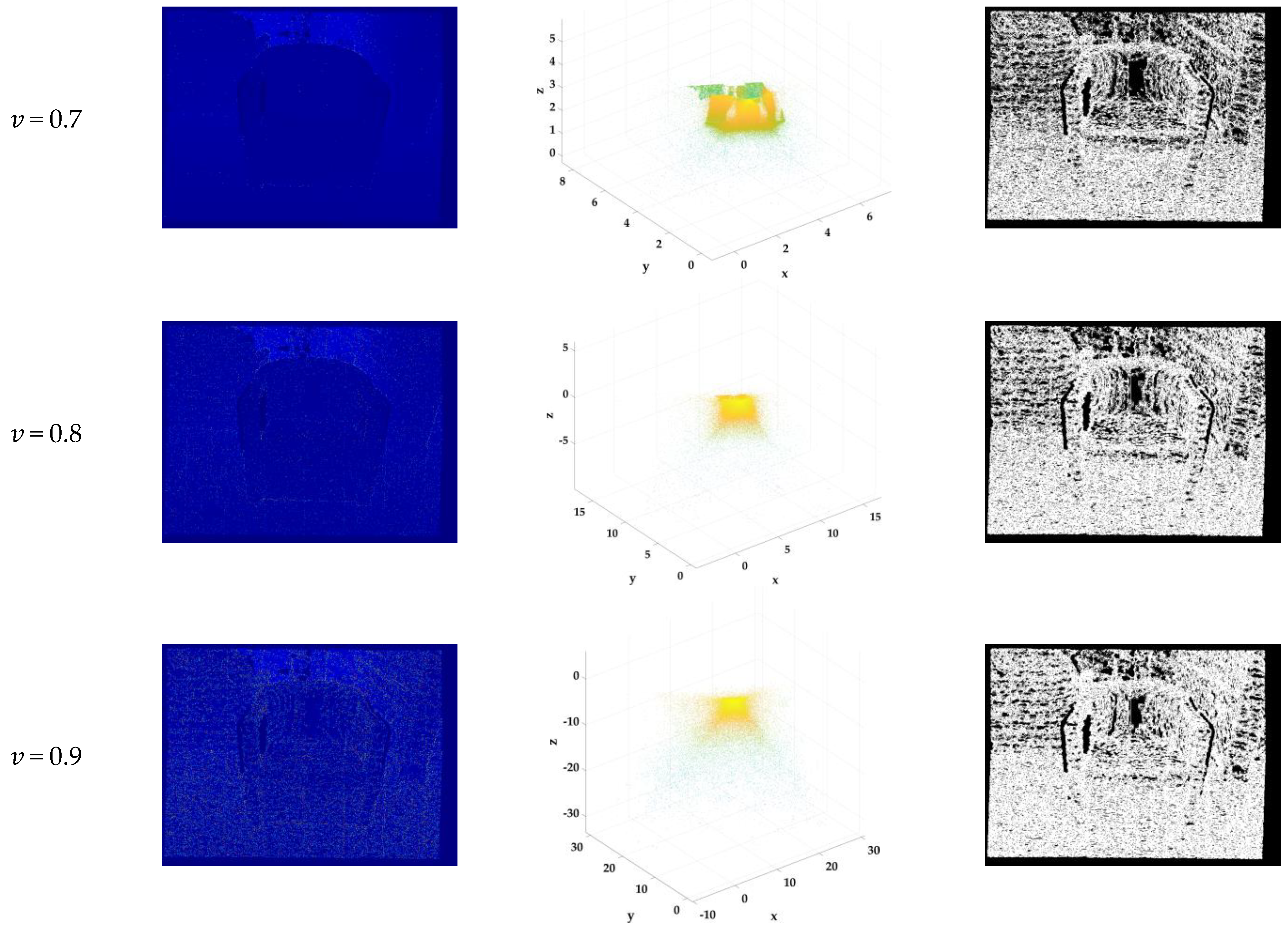
Equation (27) is applied to perform fractional differential enhancement of the depth image. The fractional order ranges from 0.1 to 0.9, and five iterations are performed. Figure 3 and Table 1 present the fractional differential enhancement effect associated with different orders.
Figure 3 shows that when the fractional differential order is greater than 0.5, excessive enhancement occurs. In contrast, when the fractional differential order is less than 0.5, the enhanced texture details are insufficiently rich. Therefore, is set to 0.5 as the optimal enhancement order, based on subjective evaluation.
4. Experimental Results and Analysis
4.1. Influence of the Number of Fractional Differential Iterations
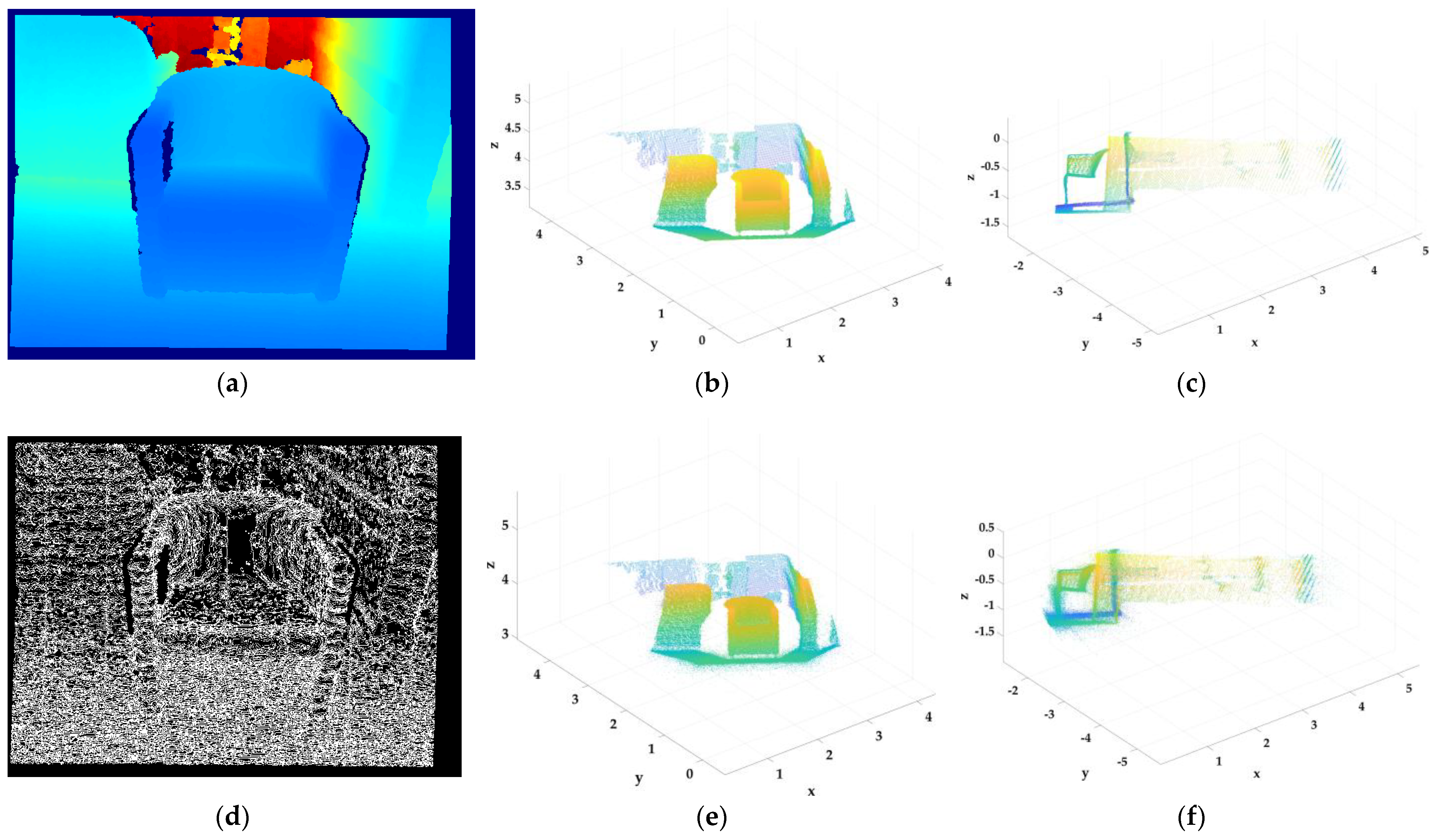
The characteristic of the fractional order is that multiple iterations of a small order can be performed to realise refined processing. Therefore, the fractional-order differential-inverse-distance-weighted enhancement model is used to enhance the depth image for 1 to 5 iterations. Dataset [24] number 00333 is used. The continuous iteration results presented in Figure 4, Figure 5, Figure 6, Figure 7 and Figure 8 indicate that the enhancement model using inverse distance weighting has the most realistic enhancement effect. Similarly, a comparison of Table 1 and Table 2 shows that the effect of one iteration of order is similar to that of five iterations of order , indicating that the performance obtained from multiple iterations of a small order is similar to that obtained from fewer iterations of a large order. Moreover, multiple iterations of the fractional differential-inverse-distance-weighting model have a uniform enhancement effect, which shows that this model can effectively enhance the texture and solve the enhancement problem of drastic changes in an edge. Thus, this enhancement model is practical for use in scenarios involving similar textural information.
4.2. Experimental Analysis and Verification of Depth Image Enhancement
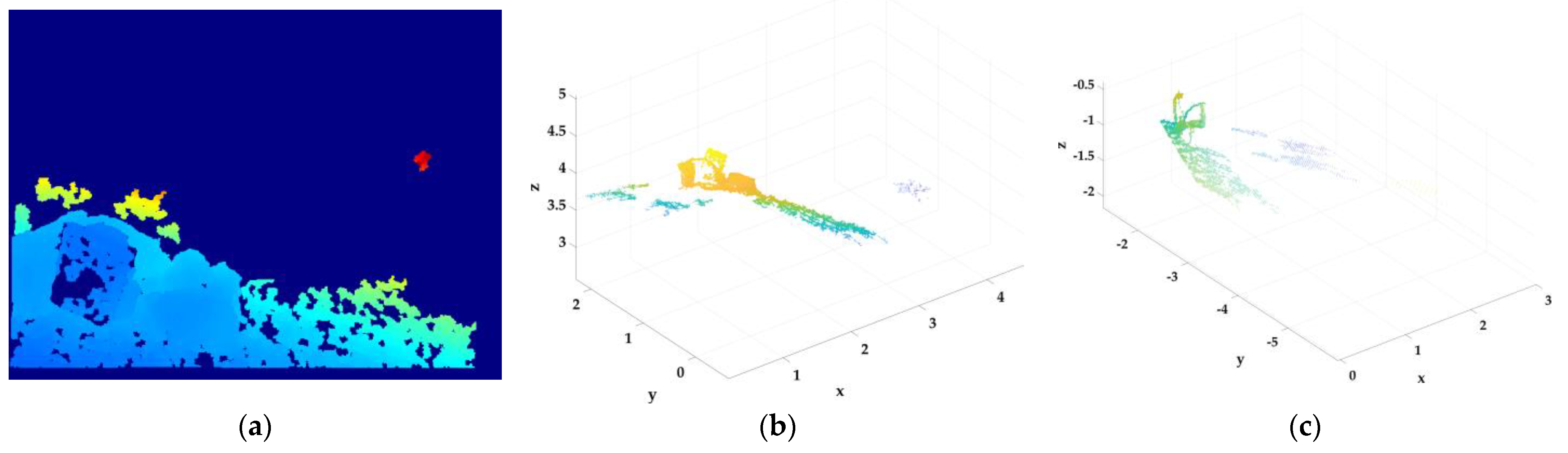
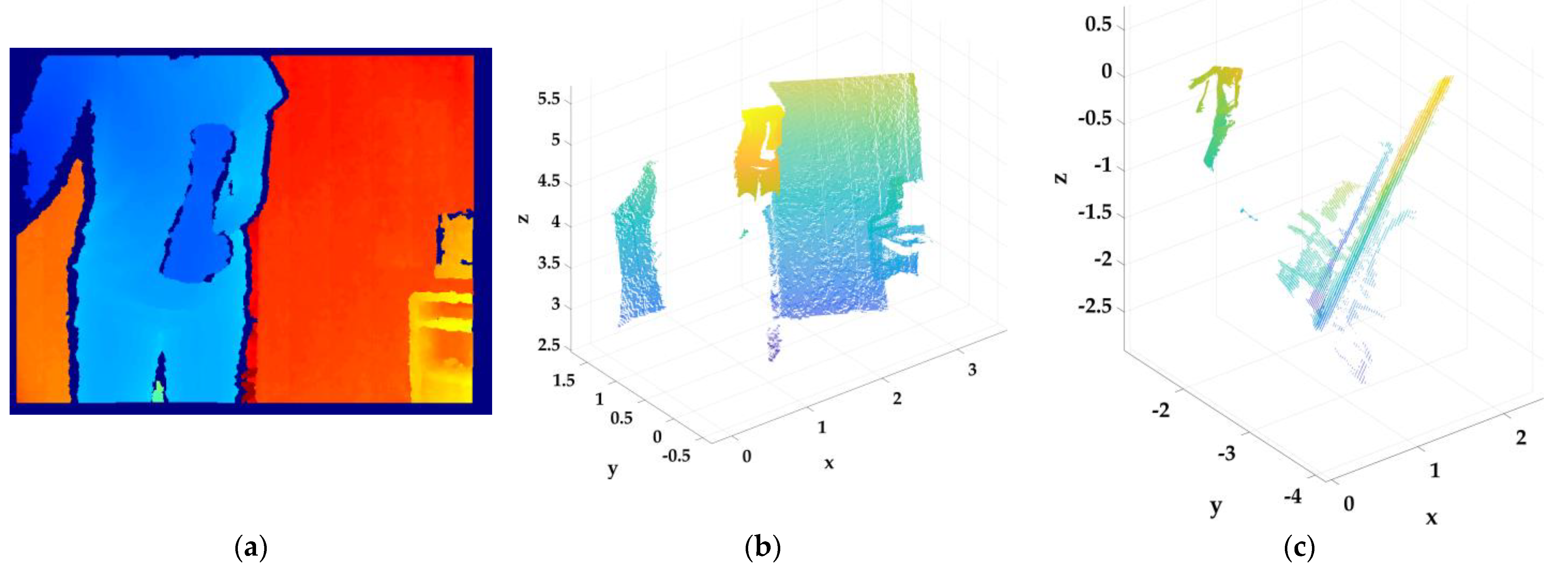
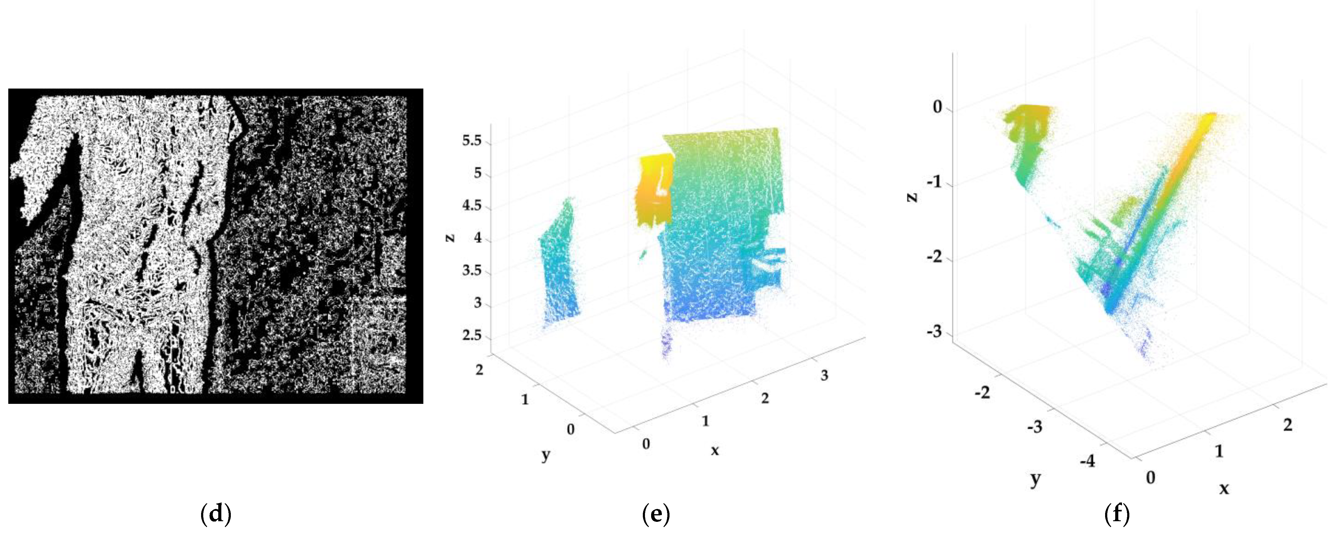
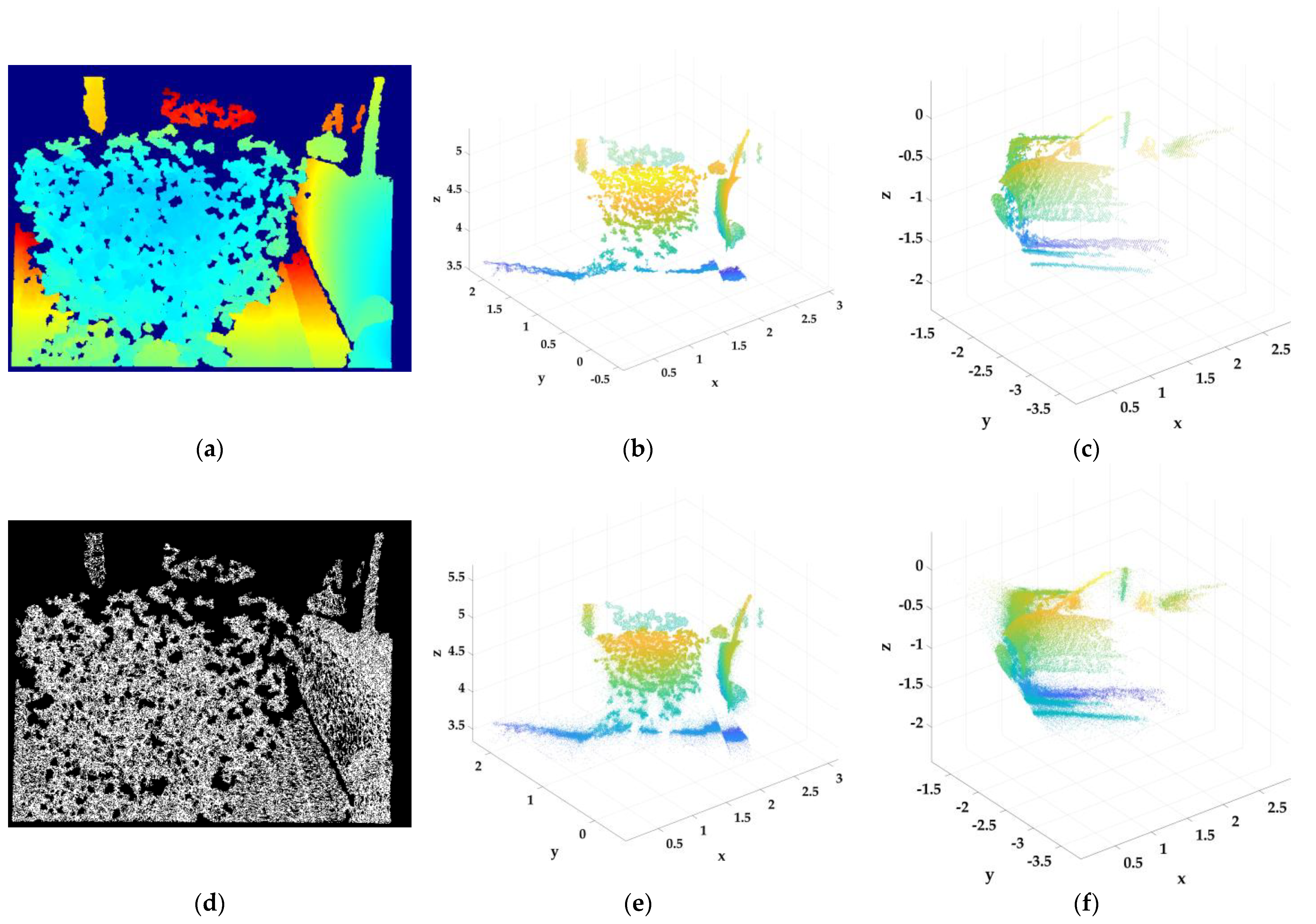
To verify the universality of the fractional differential-inverse-distance-weighted enhancement model, it is used to enhance depth images with different levels of textural information. Figure 9, Figure 10, Figure 11, Figure 12, Figure 13, Figure 14, Figure 15 and Figure 16 show the enhancement results for the depth images. These confirm that the model is universal, can achieve excellent textural enhancement effects even after many iterations, and exhibits high robustness.
In different environments, the textural information can be effectively enhanced through multiple iterations, and the enhancement amplitude of the textural information can be adjusted by modifying the number of iterations. The experimental results verify that the model selectively enhances textural information by optimising the order and the number of iterations. Moreover, the edge information of a depth image is retained after the enhancement process, which indicates that the model can effectively distinguish edge information from textural information and thereby achieve selective enhancement.
5. Discussion
Based on an examination of the existing depth image enhancement methods, a novel depth image enhancement algorithm based on a fractional differential is devised. The fractional differential-inverse-distance-weighted enhancement method is developed to solve the problem associated with high-frequency noise in fractional differential enhancement. First, image enhancement is performed based on fractional differentiation to effectively enhance the quality of a depth image. The contouring and high-frequency details of a depth image are enhanced by constructing a fractional differential mask for convolution. However, point cloud observation shows that this method introduces certain high-frequency noise at an edge. Thus, the image directly enhanced by fractional differentiation cannot be used for 3D reconstruction. Second, inverse distance weighting is applied to improve the weighted calculation of the convolution result of fractional differentiation. The improved fractional-order differential-inverse-distance-weighting algorithm can alleviate the high-frequency noise problem while maintaining the edge features of an enhanced depth image. The distance between the interpolation point and sample point is used as the weight factor to calculate the convolution result. The distance of the sample points is inversely proportional to the weight assigned in the inverse distance weighting process. The accuracy and smoothness of the resulting data are increased by the introduction of fractional filtering through the interpolation function. The experimental results show that the enhancement effect of the fractional differential-inverse-distance-weighting model is realistic and that uniform enhancement can be achieved, even after multiple iterations.
In summary, the effectiveness and superiority of depth image enhancement based on a fractional differential are demonstrated through theoretical and experimental studies, and a fractional differential-inverse-distance-weighted enhancement method is developed to solve the problems associated with fractional differential enhancement. This novel approach represents the first attempt at integrating a fractional differential into depth image enhancement and is an effective solution for depth image enhancement. For example, in the fields of medical image processing, machine vision, and autonomous driving, and compared with current methods, this algorithm could provide clearer depth images for more accurate recognition of objects and scenes.
Depth images have a wide range of practical applications, such as in 3D modelling, robot navigation, and virtual reality. Therefore, future research directions could include and verify the utility of the fractional differential enhancement algorithm in practical application scenarios and explore more efficient algorithms. First, depth image enhancement should be further combined with the depth image data required for an actual scene, and the algorithm should be applied to a scene requiring additional textural information for its depth image. Second, as the algorithm is not efficient enough to achieve real-time depth image enhancement, further research on the computational speed of the algorithm is an important future research direction. The algorithm can be implemented using a graphics processor or neural network processing unit to enable real-time depth image enhancement. Finally, the effect of the algorithm on 3D reconstruction after depth image enhancement and the 3D reconstruction of depth images with more abundant textural information than those in this study must be explored in future studies.
Author Contributions
Conceptualization, T.H., X.L. and C.W.; methodology, T.H. and X.W.; software, T.H. and D.X.; formal analysis, T.H. and X.W.; data curation, X.W. and D.X.; writing—original draft preparation, T.H. and X.W.; writing—review and editing, T.H., X.L. and C.W.; funding acquisition, X.L. and C.W. All authors have read and agreed to the published version of the manuscript.
Funding
This research was funded by National Key R&D Program of China, grant number 2022YFC3803702.
Data Availability Statement
Not applicable.
Conflicts of Interest
The authors declare no conflict of interest.
References
- Murayama, M.; Higashiyama, T.; Harazono, Y.; Ishii, H.; Shimoda, H.; Okido, S.; Taruta, Y. Depth Image Noise Reduction and Super-Resolution by Pixel-Wise Multi-Frame Fusion. IEICE Trans. Inf. Syst. 2022, E105-D, 1211–1224. [Google Scholar] [CrossRef]
- Zhang, X.-F.; Yan, H. Image Denoising and Enhancement Algorithm Based on Median Filtering and Fractional-order Filtering. J. Northeast. Univ. Nat. Sci. 2020, 41, 482–487. [Google Scholar]
- Nandal, S.; Kumar, S. Image Denoising Using Fractional Quaternion Wavelet Transform. In Proceedings of the 2nd International Conference on Computer Vision & Image Processing: CVIP 2017; Springer: Singapore, 2018; Volume 2. [Google Scholar] [CrossRef]
- Shanmugavadivu, P.; Sivakumar, V. Fractal Dimension Based Texture Analysis of Digital Images. Procedia Eng. 2012, 38, 2981–2986. [Google Scholar] [CrossRef] [Green Version]
- Zhou, D.; Wang, R.; Lu, J.; Zhang, Q. Depth Image Super Resolution Based on Edge-Guided Method. Appl. Sci. 2018, 8, 298. [Google Scholar] [CrossRef] [Green Version]
- Hui, T.-W.; Ngan, K.N. Depth enhancement using RGB-D guided filtering. In Proceedings of the 2014 IEEE International Conference on Image Processing (ICIP), Paris, France, 27–30 October 2014; pp. 3832–3836. [Google Scholar]
- Senthilkumaran, N.; Thimmiaraja, J. Histogram Equalization for Image Enhancement Using MRI Brain Images. In Proceedings of the 2014 World Congress on Computing and Communication Technologies, Trichirappalli, India, 27 February–1 March 2014; pp. 80–83. [Google Scholar]
- Wang, Z.; Lv, G.Q.; Feng, Q.B.; Wang, A.T.; Ming, H. Resolution priority holographic stereogram based on integral imaging with enhanced depth range. Opt. Express 2019, 27, 2689–2702. [Google Scholar] [CrossRef] [PubMed]
- Gupta, A.; Kumar, S. Generalized framework for the design of adaptive fractional-order masks for image denoising. Digit. Signal Process. 2022, 121, 103305. [Google Scholar] [CrossRef]
- Zhang, X.; He, H.; Zhang, J.-X. Multi-focus image fusion based on fractional-order differentiation and closed image matting. ISA Trans. 2022, 129, 703–714. [Google Scholar] [CrossRef] [PubMed]
- Harjule, P.; Tokir, M.M.; Mehta, T.; Gurjar, S.; Kumar, A.; Agarwal, B. Texture Enhancement of Medical Images for Efficient Disease Diagnosis with Optimized Fractional Derivative Masks. J. Comput. Biol. 2022, 29, 545–564. [Google Scholar] [CrossRef] [PubMed]
- Zhang, X.; Liu, R.; Ren, J.; Gui, Q. Adaptive fractional image enhancement algorithm based on rough set and particle swarm optimization. Fractal Fract. 2022, 6, 100. [Google Scholar] [CrossRef]
- Zhang, X.; Dai, L. Image enhancement based on rough set and fractional-order differentiator. Fractal Fract. 2022, 6, 214. [Google Scholar] [CrossRef]
- Zhang, L.; Jia, Z.; Koefoed, L.; Yang, J.; Kasabov, N. Remote sensing image enhancement based on the combination of adaptive nonlinear gain and the PLIP model in the NSST domain. Multimed. Tools Appl. 2020, 79, 13647–13665. [Google Scholar] [CrossRef]
- Liu, X.; Pedersen, M.; Wang, R. Survey of natural image enhancement techniques: Classification, evaluation, challenges, and perspectives. Digit. Signal Process. 2022, 127, 103547. [Google Scholar] [CrossRef]
- Hacini, M.; Hachouf, F.; Charef, A. A bi-directional fractional-order derivative mask for image processing applications. IET Image Process. 2020, 14, 2512–2524. [Google Scholar] [CrossRef]
- Li, M.M.; Li, B.Z. A Novel Active Contour Model for Noisy Image Segmentation Based on Adaptive Fractional-order Differentiation. IEEE Trans. Image Process. 2020, 29, 9520–9531. [Google Scholar] [CrossRef]
- Balochian, S.; Baloochian, H. Edge detection on noisy images using Prewitt operator and fractional-order differentiation. Multimed. Tools Appl. 2020, 81, 9759–9770. [Google Scholar] [CrossRef]
- Yu, L.; Zeng, Z.; Wang, H.; Pedrycz, W. Fractional-order differentiation based sparse representation for multi-focus image fusion. Multimed. Tools Appl. 2022, 81, 4387–4411. [Google Scholar] [CrossRef]
- Pan, X.; Zhu, J.; Yu, H.; Chen, L.; Liu, Y.; Li, L. Robust corner detection with fractional calculus for magnetic resonance imaging. Biomed. Signal Process. Control. 2021, 63, 102112. [Google Scholar] [CrossRef]
- Xu, L.; Huang, G.; Chen, Q. -L.; Qin, H.-Y.; Men, T.; Pu, Y.-F. An improved method for image denoising based on fractional-order integration. Front. Inf. Technol. Electron. Eng. 2020, 21, 1485–1493. [Google Scholar] [CrossRef]
- Huang, G.; Xu, L.; Chen, Q. -L.; Pu, Y.-F. Research on image denoising based on time-space fractional partial differential equations. Xi Tong Gong Cheng Yu Dian Zi Ji Shu/Syst. Eng. Electron. 2012, 34, 1741–1752. [Google Scholar]
- Pu, Y. -F.; Wang, W.X. Fractional differential masks of digital image and their numerical implementation algorithms. Acta Autom. Sin. 2007, 33, 1128–1135. [Google Scholar]
- Choi, S.; Zhou, Q.Y.; Miller, S.; Koltun, V. A Large Dataset of Object Scans. arXiv 2016, arXiv:1602.02481. [Google Scholar]
Figure 1.
Fractional differential mask.

Figure 2.
Fractional differential image enhancement. (a) Pseudo-colour image of the depth image. (b) Front view and (c) side view of the point clouds.
Figure 2.
Fractional differential image enhancement. (a) Pseudo-colour image of the depth image. (b) Front view and (c) side view of the point clouds.


Figure 3.
Fractional differential enhancement effect.


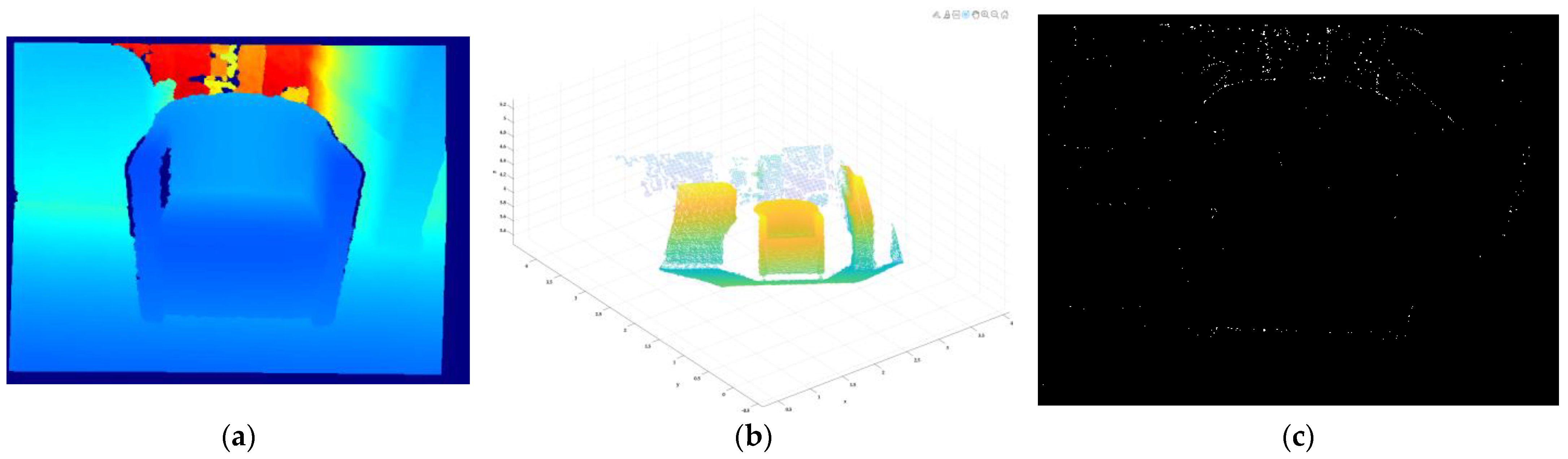
Figure 4.
Results of one iteration of fractional differential enhancement (, PSNR = 64.680 dB). (a) Pseudo-colour image; (b) front view of the point cloud (after one-iteration enhancement); (c) residual image of the enhanced result.
Figure 4.
Results of one iteration of fractional differential enhancement (, PSNR = 64.680 dB). (a) Pseudo-colour image; (b) front view of the point cloud (after one-iteration enhancement); (c) residual image of the enhanced result.

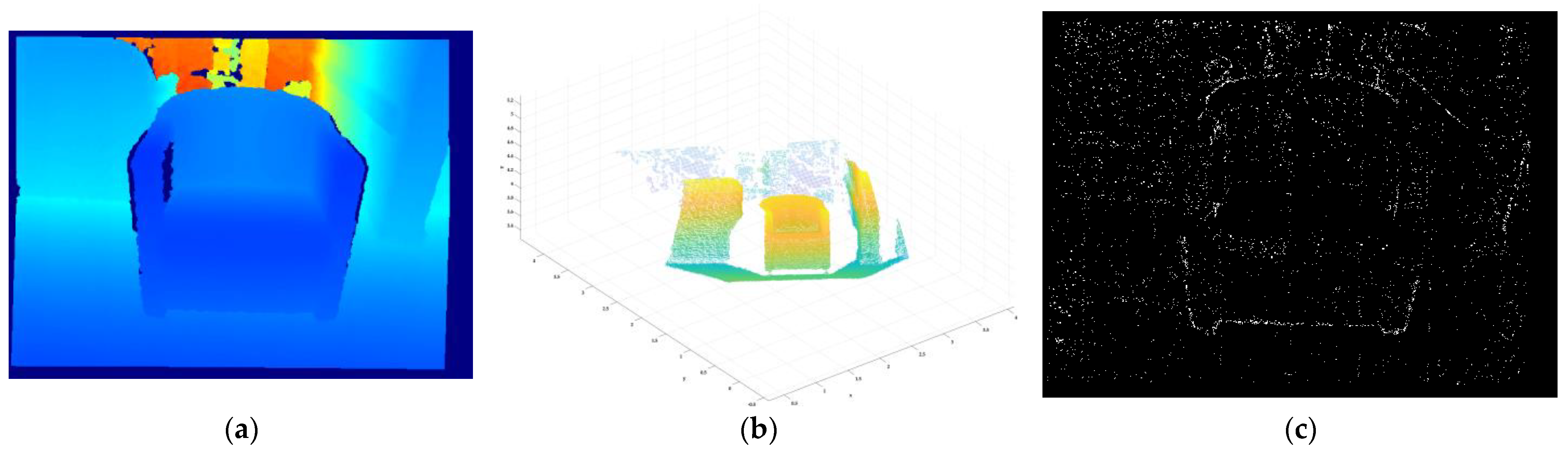
Figure 5.
Results of two iterations of fractional differential enhancement (, PSNR = 53.476 dB). (a) Pseudo-colour image; (b) front view of the point cloud (after one-iteration enhancement); (c) residual image of the enhanced result.
Figure 5.
Results of two iterations of fractional differential enhancement (, PSNR = 53.476 dB). (a) Pseudo-colour image; (b) front view of the point cloud (after one-iteration enhancement); (c) residual image of the enhanced result.

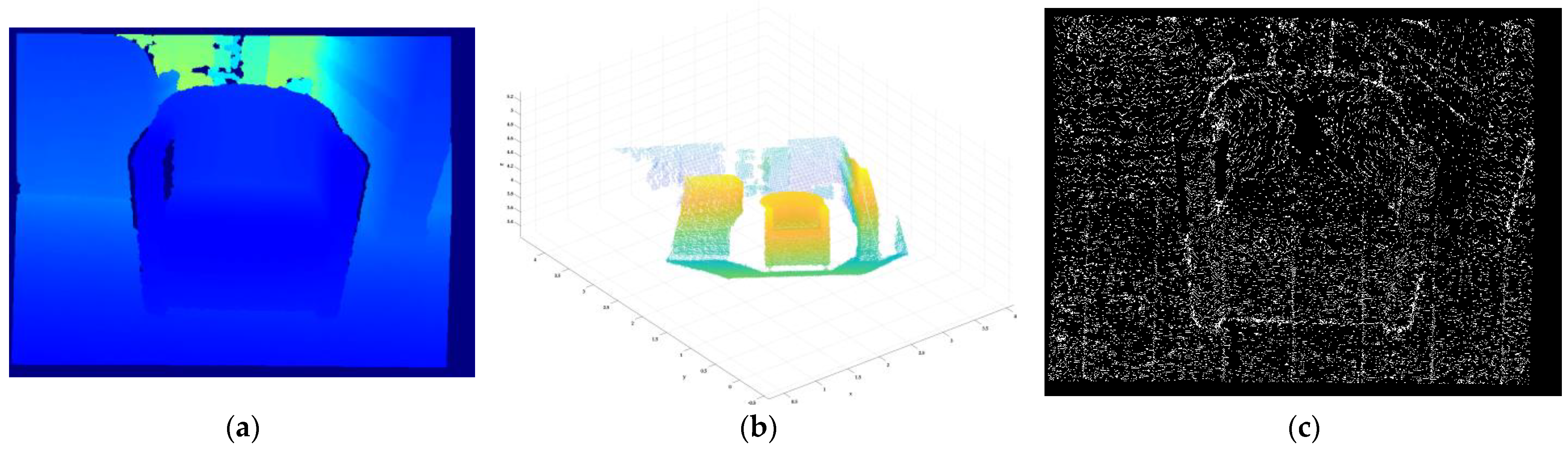
Figure 6.
Results of three iterations of fractional differential enhancement (, PSNR = 43.639 dB). (a) Pseudo-colour image; (b) front view of the point cloud (after one-iteration enhancement); (c) residual image of the enhanced result.
Figure 6.
Results of three iterations of fractional differential enhancement (, PSNR = 43.639 dB). (a) Pseudo-colour image; (b) front view of the point cloud (after one-iteration enhancement); (c) residual image of the enhanced result.

Figure 7.
Results of four iterations of fractional differential enhancement (, PSNR = 34.621 dB). (a) Pseudo-colour image; (b) front view of the point cloud (after one-iteration enhancement); (c) residual image of the enhanced result.
Figure 7.
Results of four iterations of fractional differential enhancement (, PSNR = 34.621 dB). (a) Pseudo-colour image; (b) front view of the point cloud (after one-iteration enhancement); (c) residual image of the enhanced result.

Figure 8.
Results of five iterations of fractional differential enhancement (, PSNR = 26.832 dB). (a) Pseudo-colour image; (b) front view of the point cloud (after one-iteration enhancement); (c) residual image of the enhanced result.
Figure 8.
Results of five iterations of fractional differential enhancement (, PSNR = 26.832 dB). (a) Pseudo-colour image; (b) front view of the point cloud (after one-iteration enhancement); (c) residual image of the enhanced result.

Figure 9.
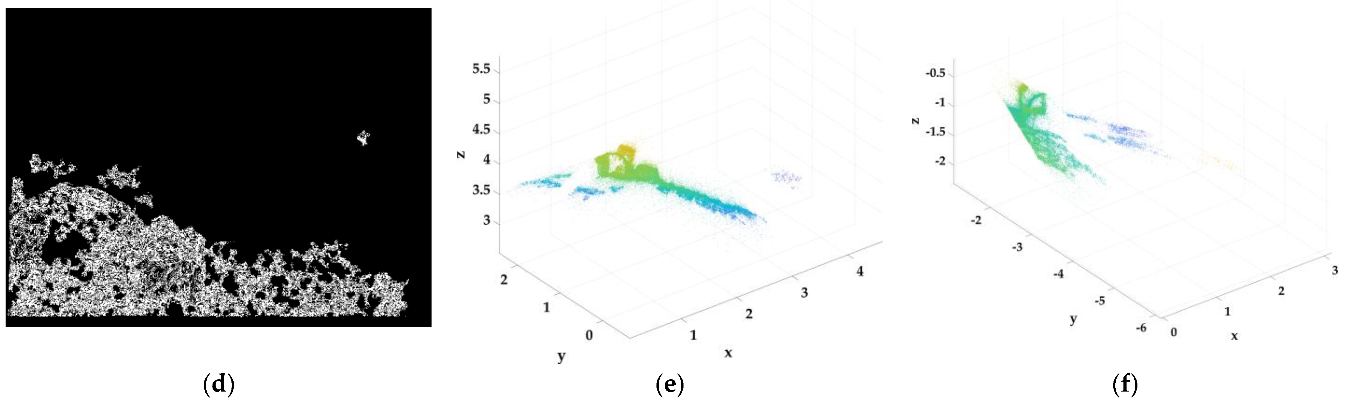
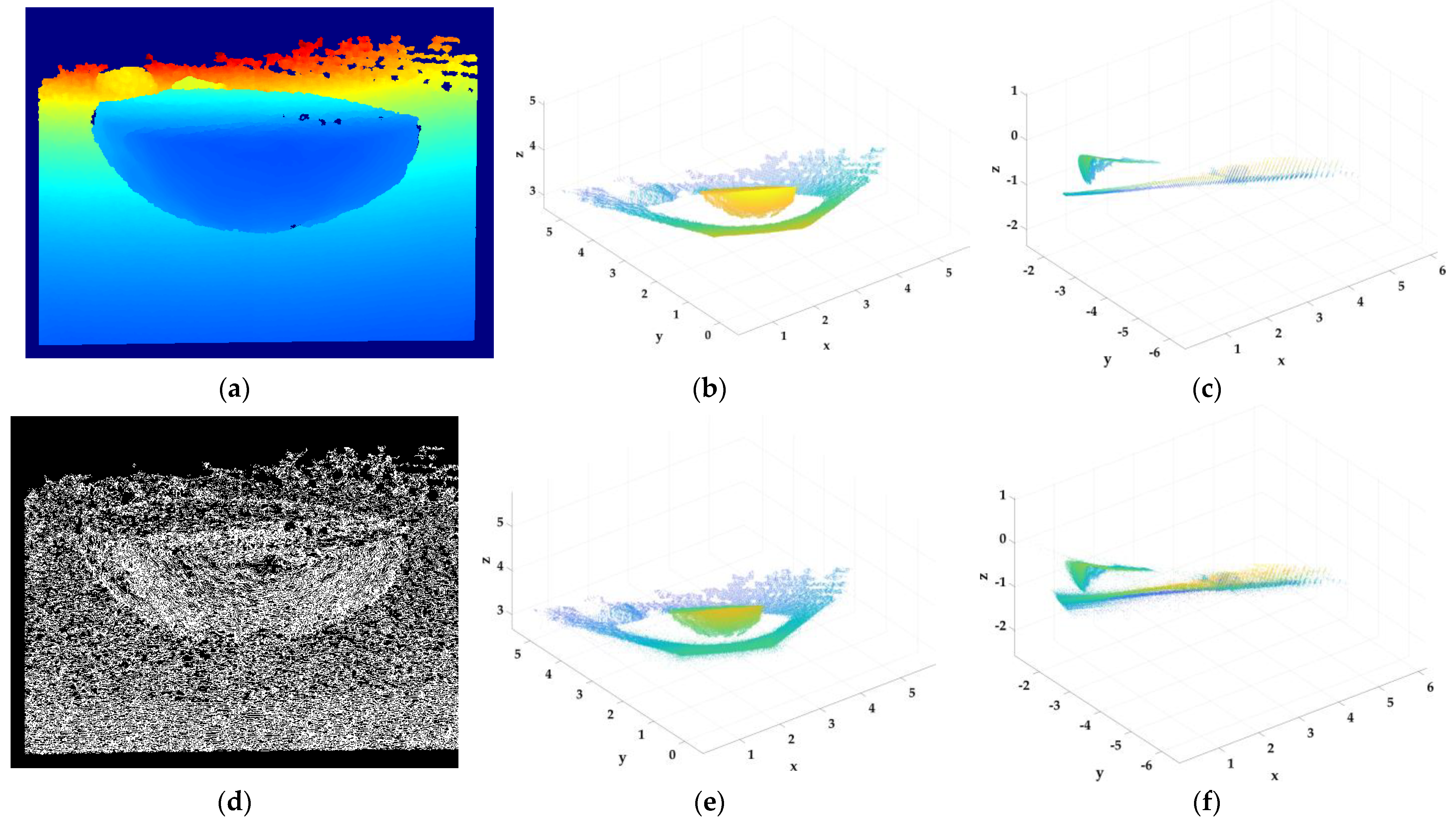
Results of five iterations of the fractional differential enhancement model (with dataset number 00333) (ν = 0.5, PSNR = 26.832 dB). (a) Pseudo-colour image; (b) front view and (c) side view of point clouds (unenhanced image); (d) residual image of the enhancement result; (e) front view and (f) side view after five-iteration enhancement.
Figure 9.
Results of five iterations of the fractional differential enhancement model (with dataset number 00333) (ν = 0.5, PSNR = 26.832 dB). (a) Pseudo-colour image; (b) front view and (c) side view of point clouds (unenhanced image); (d) residual image of the enhancement result; (e) front view and (f) side view after five-iteration enhancement.

Figure 10.
Results of five iterations of the fractional differential enhancement model (with dataset number 02350) (ν = 0.5, PSNR = 35.606 dB). (a) Pseudo-colour image; (b) front view and (c) side view of point clouds (unenhanced image); (d) residual image of the enhancement result; (e) front view and (f) side view after five-iteration enhancement.


Figure 11.
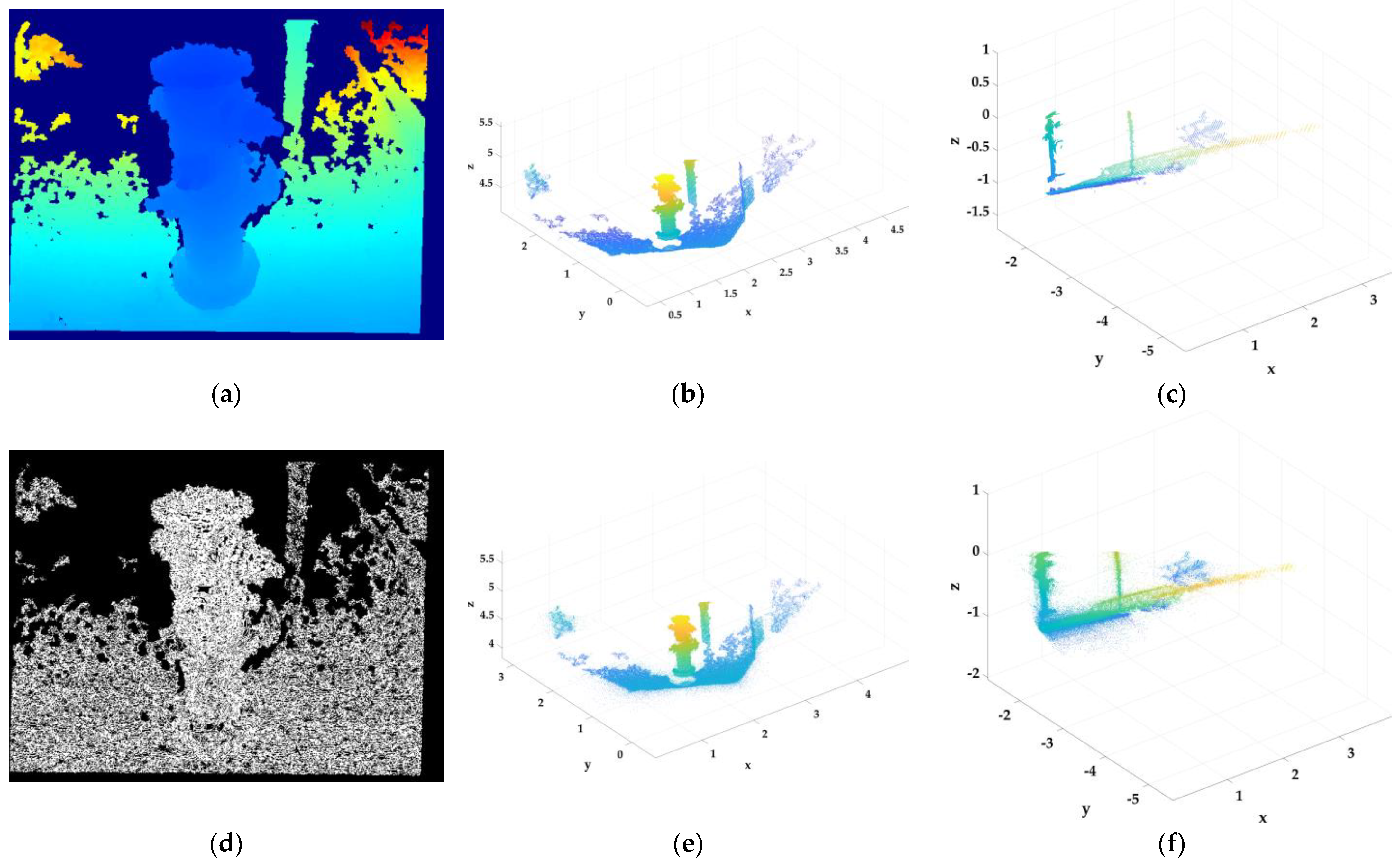
Results of five iterations of the fractional differential enhancement model (with dataset number 03236) (ν = 0.5, PSNR = 29.931 dB). (a) Pseudo-colour image; (b) front view and (c) side view of point clouds (unenhanced image); (d) residual image of the enhancement result; (e) front view and (f) side view after five-iteration enhancement.
Figure 11.
Results of five iterations of the fractional differential enhancement model (with dataset number 03236) (ν = 0.5, PSNR = 29.931 dB). (a) Pseudo-colour image; (b) front view and (c) side view of point clouds (unenhanced image); (d) residual image of the enhancement result; (e) front view and (f) side view after five-iteration enhancement.

Figure 12.
Results of five iterations of the fractional differential enhancement model (with dataset number 03528) (ν = 0.5, PSNR = 31.189 dB). (a) Pseudo-colour image; (b) front view and (c) side view of point clouds (unenhanced image); (d) residual image of the enhancement result; (e) front view and (f) side view after five-iteration enhancement.

Figure 13.
Results of five iterations of the fractional differential enhancement model (with dataset number 04797) (ν = 0.5, PSNR = 32.671 dB). (a) Pseudo-colour image; (b) front view and (c) side view of point clouds (unenhanced image); (d) residual image of the enhancement result; (e) front view and (f) side view after five-iteration enhancement.

Figure 14.
Results of five iterations of the fractional differential enhancement model (with dataset number 05989) (ν = 0.5, PSNR = 34.016 dB). (a) Pseudo-colour image; (b) front view and (c) side view of point clouds (unenhanced image); (d) residual image of the enhancement result; (e) front view and (f) side view after five-iteration enhancement.

Figure 15.
Results of five iterations of the fractional differential enhancement model (with dataset number 09860) (ν = 0.5, PSNR = 28.462 B). (a) Pseudo-colour image; (b) front view and (c) side view of point clouds (unenhanced image); (d) residual image of the enhancement result; (e) front view and (f) side view after five-iteration enhancement.


Figure 16.
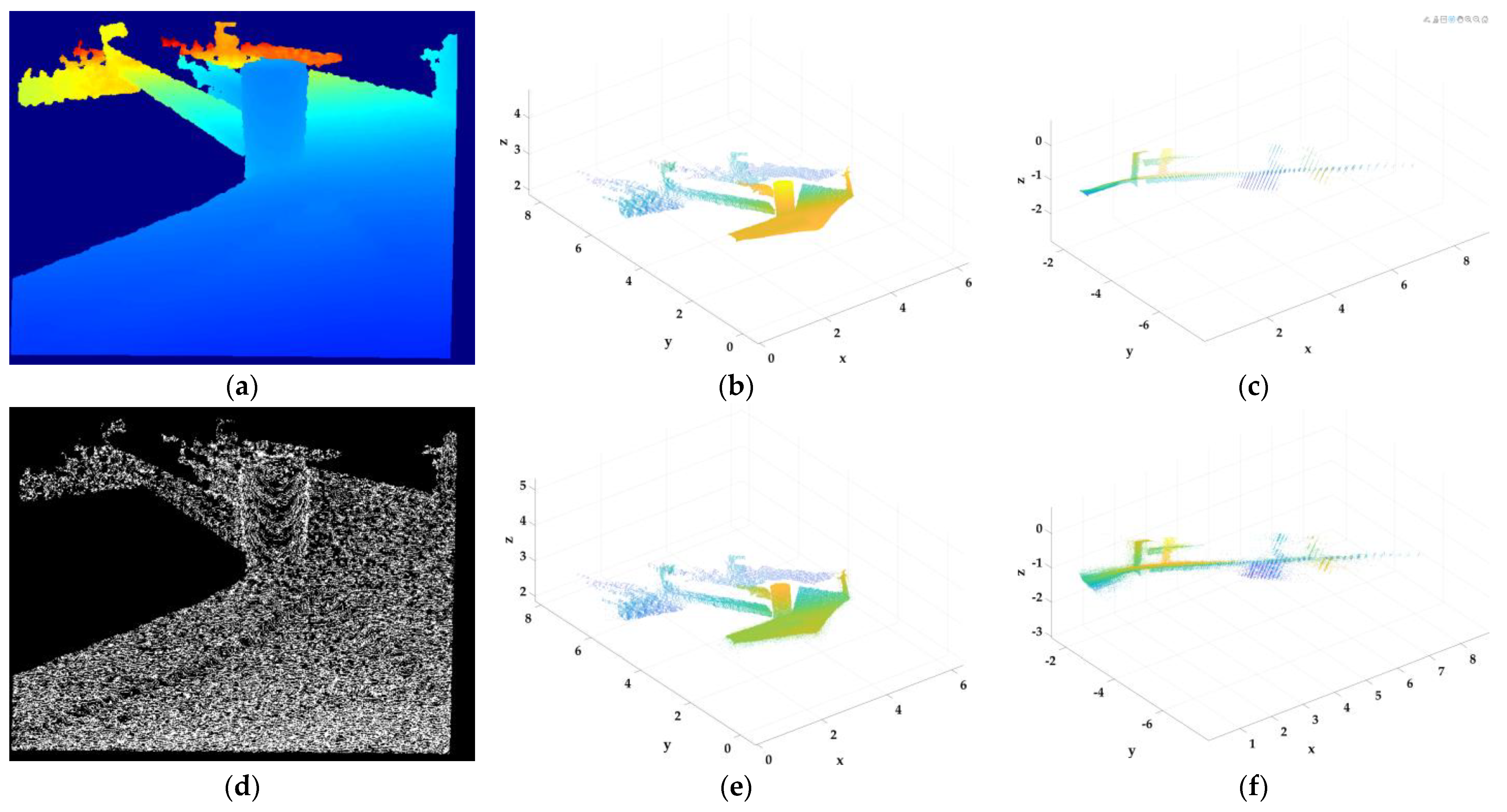
Results of five iterations of the fractional differential enhancement model (with dataset number 08343) (ν = 0.5, PSNR = 29.913 dB). (a) Pseudo-colour image; (b) front view and (c) side view of point clouds (unenhanced image); (d) residual image of the enhancement result; (e) front view and (f) side view after five-iteration enhancement.
Figure 16.
Results of five iterations of the fractional differential enhancement model (with dataset number 08343) (ν = 0.5, PSNR = 29.913 dB). (a) Pseudo-colour image; (b) front view and (c) side view of point clouds (unenhanced image); (d) residual image of the enhancement result; (e) front view and (f) side view after five-iteration enhancement.


Table 1.
Enhancement effect of fractional differential of different orders.
| Fractional Order | Enhancement Effect (PSNR) |
|---|---|
| 61.872 dB | |
| 54.026 dB | |
| 44.996 dB | |
| 35.875 dB | |
| 26.832 dB | |
| 19.698 dB | |
| 13.143 dB | |
| 3.532 dB | |
| 0.135 dB |
Table 2.
Enhancement effect of fractional differential with various numbers of iterations.
| Iterations | Enhancement Effect (PNSR) |
|---|---|
| 1 | 64.680 dB |
| 2 | 53.476 dB |
| 3 | 43.649 dB |
| 4 | 34.621 dB |
| 5 | 26.832 dB |
Disclaimer/Publisher’s Note: The statements, opinions and data contained in all publications are solely those of the individual author(s) and contributor(s) and not of MDPI and/or the editor(s). MDPI and/or the editor(s) disclaim responsibility for any injury to people or property resulting from any ideas, methods, instructions or products referred to in the content. |
© 2023 by the authors. Licensee MDPI, Basel, Switzerland. This article is an open access article distributed under the terms and conditions of the Creative Commons Attribution (CC BY) license (https://creativecommons.org/licenses/by/4.0/).
Share and Cite
MDPI and ACS Style
Huang, T.; Wang, X.; Xie, D.; Wang, C.; Liu, X. Depth Image Enhancement Algorithm Based on Fractional Differentiation. Fractal Fract. 2023, 7, 394. https://doi.org/10.3390/fractalfract7050394
AMA Style
Huang T, Wang X, Xie D, Wang C, Liu X. Depth Image Enhancement Algorithm Based on Fractional Differentiation. Fractal and Fractional. 2023; 7(5):394. https://doi.org/10.3390/fractalfract7050394
Chicago/Turabian StyleHuang, Tingsheng, Xinjian Wang, Da Xie, Chunyang Wang, and Xuelian Liu. 2023. "Depth Image Enhancement Algorithm Based on Fractional Differentiation" Fractal and Fractional 7, no. 5: 394. https://doi.org/10.3390/fractalfract7050394