Bernoulli-Type Spectral Numerical Scheme for Initial and Boundary Value Problems with Variable Order

Abstract

This manuscript is devoted to using Bernoulli polynomials to establish a new spectral method for computing the approximate solutions of initial and boundary value problems of variable-order fractional differential equations. With the help of the aforementioned method, some operational matrices of variable-order integration and differentiation are developed. With the aid of these operational matrices, the considered problems are converted to algebraic-type equations, which can be easily solved using computational software. Various examples are solved by applying the method described above, and their graphical presentation and accuracy performance are provided.

1. Introduction

Fractional calculus provides generalization to classical calculus. The history of fractional calculus is given in detail in [1]. Fractional calculus is the basic tool for modeling many real-world problems. Fractional-order integral and differential equations (FOIDEs) have many applications in almost every field of science and engineering: for example, the aforementioned area is increasingly being used in many branches of physics, such as solid physics [2], statistical physics [3], fluid mechanics [4], and viscoelasticity [5]. In the same way, in other branches of science—including biology, chemistry, and economics—fractional calculus concepts have been used. Here, we cite some famous works, where the concepts of the fractional calculus were used to investigate real world problems, as in [6,7,8,9]. Most FOIDEs cannot be solved analytically; therefore, numerical schemes and procedures have been developed by researchers for the solutions to FOIDEs. These schemes and procedures include the transformation scheme [10], the iteration procedure [11], the perturbation scheme [12], the Tau procedure [13,14], and the collocation scheme [15].

We note that the use of numerical methods based on the operational matrices of orthogonal polynomials, in order to solve various problems related to differential and integral equations of arbitrary order on finite and infinite intervals, produced highly accurate solutions for the aforementioned equations. Due to these important applications, orthogonal functions and polynomial series have received considerable attention, in dealing with various problems related to differential equations of arbitrary orders. Researchers have utilized various orthogonal polynomials introduced by Legendre, Chebyshev, Jacobi, and Bernstein to create matrices corresponding to fractional order integration and differentiation, called operational matrices (see [16,17,18]). The main characteristic of the aforementioned matrices is to reduce the problems under consideration, of fractional integration or differentiation, to a system of algebraic equations: hence, the said procedure greatly simplifies the problem for its numerical solution. In the same way, the operational matrices of fractional derivatives and integrals have also been presented for orthogonal Laguerre and modified generalized Laguerre polynomials, and their use with numerical techniques for solving various problems of fractional calculus on a semi-infinite interval; for further details, refer to [19].

Recently, researchers have observed that there exist different dynamical problems with FOIDEs that are time- and space-dependent. These problems have attracted the attention of researchers to variable-order calculus. Samko and his co-authors introduced variable-order calculus for the first time in 1993 [20]. Variable-order calculus is the generalization of fractional calculus, and it is used for the solutions of some complicated dynamical problems. The definitions of arbitrary order integration and differentiation, introduced by Riemann–Liouville and Caputo, have been extended to variable order.

It is very difficult to obtain analytical solutions to various variable-order integral and differential equations (VOIDEs), due to the complex nature of the variable order. On the other hand, numerical solutions are also very difficult to obtain, because of the kernel of the operators of variable-order integration and differentiation having variable power: due to this fact, very few methods have been developed for numerical solutions to VOIDEs. Those methods which have been developed include the second-order Runge–Kutta method, introduced by Soon [21] and his co-authors to study the variable viscoelasticity oscillator problem. The finite difference approximation method was used by Lin et al. [22] to investigate variable-order diffusion problems. Zhuang et al. [23] used the Euler approximation method to compute approximate solutions to advanced diffusion problems. Chen et al. [24] developed a numerical scheme with high spatial accuracy for a variable-order anomalous sub-diffusion equation. Recently, Amin et al. [25] extended the wavelet method for a class of variable order linear integro-differential equations. In the same vein, some authors [26] have recently studied various classes of variable-order problems by using a non-orthogonal basis.

Bernoulli polynomials have been used to obtain numerical solutions to various problems with fractional orders. For instance, Keshavarz et al. [27] used the operational matrices method to obtain the numerical solution for fractional optimal control problems via Bernoulli polynomials. Recently, Bernoulli polynomials have been used to study various problems of fractional calculus for numerical solutions (see [28,29,30]). For further properties and applications of Bernoulli polynomials, readers should refer to [31,32,33]. The same operational matrices of Bernoulli polynomials have been extended to variable-order optimal control problems by Nemati et al. [34].

Dealing with boundary value problems for numerical results is currently an attractive area of research. In addition, the investigation of boundary value problems under variable order has hitherto very rarely been considered. On the other hand, left and right fractional differential operators are also attracting much attention, as they appear as the Euler–Lagrange equations in the study of variational principles (see [35]). We know that fractional differential equations are widely used for modeling anomalous diffusion in porous media, in which particles have been observed to spread at a rate that was incompatible with classical Brownian motion. For such purposes, the Riesz fractional derivative has been shown to be more attractive than the left-sided derivative, as it is able to take into account contributions from both sides of the domain (see [36,37]). The aforementioned differential operator is a linear combination of the left- and right-sided derivatives, hence resulting in a fractional differential operator centrally symmetric on finite domains. While the aforementioned derivative is commonly used as a left and right Riemann–Liouville derivative of fractional order, to model fractional diffusion, the Riesz–Caputo derivative seems more suitable for avoiding nonphysical issues (see [38]). Very recently, Blaszczyk et al. [39] investigated some applications of the Riesz–Caputo fractional derivative of variable order with fixed memory. In the same way, Pitolli et al. [40] investigated approximation of the Riesz–Caputo derivative by cubic splines. The aforementioned differential operator of variable order, depending on a time variable with fixed memory a, is defined as

$$\begin{array}{c}\hfill {}_{t-a}^{RC}{\mathbf{D}}_{t+a}^{v\left(t\right)}z\left(t\right)=\frac{1}{2}\left[{}_{t-a}^C{\mathbf{D}}_t^{v\left(t\right)}z\left(t\right)+{(-1)}^n{}_t^C{\mathbf{D}}_{t+a}^{v\left(t\right)}z\left(t\right)\right],\end{array}$$

where

$$\begin{array}{ccc}\hfill {}_{t-a}^C{\mathbf{D}}_t^{v\left(t\right)}z\left(t\right)& =& \frac{1}{\Gamma (n-v(t\left)\right)}{\int }_{t-a}^t{(t-\tau )}^{n-v\left(t\right)-1}{z}^{\left(n\right)}\left(\tau \right)d\tau ,n-1<v\left(t\right)<n,\hfill \\ \hfill {}_t^C{\mathbf{D}}_{t+a}^{v\left(t\right)}z\left(t\right)& =& \frac{1}{\Gamma (n-v(t\left)\right)}{\int }_t^{t+a}{(\tau -t)}^{n-v\left(t\right)-1}{z}^{\left(n\right)}\left(\tau \right)d\tau ,n-1<v\left(t\right)<n.\hfill \end{array}$$

Inspired by the above discussion, this paper is devoted to presenting an algorithm using the aforementioned concept of fractional-order Bernoulli polynomials, and using this approximation to solve initial and boundary value problems with variable-order derivatives depending on time. Keeping in mind the importance of the left operator of variable order, we will use it in our results. Our first considered problem with the initial condition is described as

$$\left\{\begin{array}{cc}\hfill & {\mathbf{D}}^{v_1\left(t\right)}y\left(t\right)+cy\left(t\right)=h\left(t\right),c\in \mathbf{R},t\in [0,1],\hfill \\ & y\left(0\right)=y_0,y_0\in \mathbf{R},\hfill \end{array}\right.$$

(1)

where $h:[0,1]\to \mathbf{R}$ is a linear continuous function, and $v_1:[0,1]\to (0,1]$ is a continuous function. In addition, we consider our second problem, under some boundary conditions, as

$$\left\{\begin{array}{cc}& {\mathbf{D}}^{v\left(t\right)}y\left(t\right)+c_1{\mathbf{D}}^{v_1\left(t\right)}y\left(t\right)+c_{2}y\left(t\right)=g\left(t\right),c_1,c_2\in \mathbf{R},t\in [0,1]\hfill \\ & y\left(0\right)=y_0,y\left(1\right)=y_1,y_0,y_1\in \mathbf{R},\hfill \end{array}\right.$$

(2)

where $g:[0,1]\to \mathbf{R}$ is a linear continuous function defined, and $v:[0,1]\to (1,2],v_1:[0,1]\to (0,1]$ are continuous functions.

We present numerical algorithms based on operational matrices for the above problems. For this purpose, we first reconstruct operational matrices for fractional-order integration and differentiation, as already derived in [34] for variable order. In addition, we also create new matrices corresponding to boundary conditions. Based on the aforementioned operational matrices, the considered problems are converted to algebraic type equations, which we solve by using Matlab, for finding the unknown vector. In this way, we obtain the required numerical solution to the problem under our consideration. Usually, the operational matrices are used in a variety of ways. Majority research work established these matrices by using collocation and discretization tools, which require extra memory consumption and more time for employment. To overcome these issues, we establish these matrices directly, an approach which had been very rarely considered. Furthermore, the operational matrix corresponding to the boundary conditions in Theorem 3 has also been newly obtained according to our information. Generally, researchers perform numerical solutions for variable order lies in $(0,1]$, and very rarely for order in $(1,2]$. In addition, using the variable-order Riemann–Liouville integral operator and the Caputo differential operator, we specify that these are the left operators. In the adopted fractional differential operators, the Caputo derivative is the most-used operator. Furthermore, the Caputo derivative is related to the Reimann–Liouville derivative by a proper relationship. Usually, Caputo has no integral operator, as the Caputo derivative is deduced from Reimann–Liouville as a special consequence. Furthermore, its geometrical interpretation can be performed like ordinary derivatives. Most of the applied problem requires fractional derivatives with proper utilization of initial conditions with known physical interpretation, especially in the theory of viscoelasticity and solid mechanics. In such cases, the Caputo approach is more applicable, because in Caputo fractional derivatives, the initial conditions are the same as those of integer-ordered differential equations, and these initial conditions have a known physical interpretation of the problem.

2. Basic Results

This section is devoted to some fundamental results of variable-order derivatives and integration. In addition, some properties of Bernoulli polynomials are presented.

Definition 1

([34,41]). The left Riemann–Liouville fractional integral of order $v\left(t\right)$ is defined as

$${}_0{\mathbf{I}}_t^{v\left(t\right)}x\left(t\right)=\frac{1}{\Gamma \lceil v\left(t\right)\rceil }{\int }_0^t{(t-k)}^{v\left(t\right)-1}x\left(k\right)dk,t>0,$$

(3)

where Γ is the Euler gamma function described as $\Gamma \left(t\right)={\int }_0^{\infty }{k}^{t-1}exp(-k)dk,t>0,$ and $\lceil ·\rceil$ is the ceiling function.

This operator obeys the following properties, as discussed in [41]:

i.

${}_0{\mathbf{I}}_t^{v\left(t\right)}(l_1{x}_1\left(t\right)+l_2{x}_2\left(t\right))=l_1{}_0{\mathbf{I}}_t^{v\left(t\right)}{x}_1\left(t\right)+l_2{}_0{\mathbf{I}}_t^{v\left(t\right)}{x}_2\left(t\right)$,

ii.

${}_0{\mathbf{I}}_t^{v_1\left(t\right)}{}_0{\mathbf{I}}_t^{v_2\left(t\right)}{=}_0{\mathbf{I}}_t^{v_1\left(t\right)+v_2\left(t\right)}x\left(t\right)$,

iii.

${}_0{\mathbf{I}}_t^{v_1\left(t\right)}{}_0{\mathbf{I}}_t^{v_2\left(t\right)}x\left(t\right){=}_0{\mathbf{I}}_t^{v_2\left(t\right)}{}_0{\mathbf{I}}_t^{v_1\left(t\right)}x\left(t\right)$,

iv.

${}_0{\mathbf{I}}_t^{v_1\left(t\right)}{t}^{\alpha }=\frac{\Gamma (\alpha +1)}{\Gamma (\alpha +1+v_1\left(t\right))}{t}^{\alpha +v_1\left(t\right)}$, $\alpha >-1$,

where $l_1$ and $l_2$ are real numbers.

Definition 2.

The left variable-order Caputo differential operator is defined as [31,34]

$$\begin{array}{cc}& {\mathbf{D}}_t^{v\left(t\right)}x\left(t\right)=\frac{1}{\Gamma \lceil n-v\left(t\right)\rceil }{\int }_0^t{(t-k)}^{n-v\left(t\right)-1}{x}^{\left(n\right)}\left(k\right)dk,n-1<v\left(t\right)\le n,t>0.\hfill \end{array}$$

(4)

For $0\le v\left(t\right)<w\left(t\right)\le n,n\in \mathbb{N}$ and $\alpha >0,$ this operator obeys the following properties, as discussed in [34,41]:

i.

${\mathbf{D}}_t^{v\left(t\right)}{}_0{\mathbf{I}}_t^{v\left(t\right)}x\left(t\right)=x\left(t\right)$,

ii.

${}_0{\mathbf{I}}_t^{v\left(t\right)}{}_0^C{\mathbf{D}}_t^{v\left(t\right)}x\left(t\right)=x\left(t\right)-{\sum }_{i=0}^{\lceil v\left(t\right)\rceil -1}{x}^{\left(i\right)}\left(0\right)\frac{t^i}{i!},t>0$

iii.

${\mathbf{D}}_t^{v\left(t\right)}{t}^{\alpha }=\left\{\begin{array}{cc}0,\hfill & \alpha <v\left(t\right),\hfill \\ \frac{\Gamma (\alpha +1)}{\Gamma (\alpha +1-v(t\left)\right)}{t}^{\alpha -v\left(t\right)},\hfill & \mathrm{otherwise},\hfill \end{array}\right.$

iv.

${}_0{\mathbf{I}}_t^{v\left(t\right)}\left(x^n\left(t\right)\right)={}_0^C{\mathbf{D}}_t^{v\left(t\right)}x\left(t\right)-{\sum }_{i=\lceil v\left(t\right)\rceil }^{n-1}{x}^i\left(0\right)\frac{t^{i-v\left(t\right)}}{\Gamma (i-v(t)+1)},t>0,$

v.

${}_0{\mathbf{I}}_t^{v\left(t\right)-w\left(t\right)}\left({}_0^C{\mathbf{D}}_t^{v\left(t\right)}\right)={}_0^C{\mathbf{D}}_t^{w\left(t\right)}x\left(t\right)-{\sum }_{i=\lceil w\left(t\right)\rceil }^{\lceil v\left(t\right)\rceil -1}{x}^i\left(0\right)\frac{t^{i-w\left(t\right)}}{\Gamma (i-w(t)+1)},t>0,$

vi.

${}_0^C{\mathbf{D}}_t^{v\left(t\right)}\mathrm{c}=0$,

vii.

${}_0^C{\mathbf{D}}_t^{v\left(t\right)}\left(l_1{x}_1\left(t\right)+l_2{x}_2\left(t\right)\right)=l_1{}_0^C{\mathbf{D}}_t^{v\left(t\right)}{x}_1\left(t\right)+l_2{}_0^C{\mathbf{D}}_t^{v\left(t\right)}{x}_2\left(t\right)$,

where $c,l_1,l_2$ are any real constants.

The Fractional-Order Bernoulli Polynomials

In this subsection, we define the fractional-order Bernoulli functions (FOBFs), and show some of their properties.

Definition 3.

The fractional-order Bernoulli polynomials ${\mathbf{B}}_i^{\gamma }\left(t\right)$ of order $i\gamma$ are defined over $[0,1]$ as [32]

$$B_i^{\gamma }\left(t\right)=\sum _{r=0}^i\left(\genfrac{}{}{0pt}{}{i}{r}\right)B_{i-r}^{\gamma }{t}^{r\gamma },t\in [0,1],$$

(5)

where $B_r^{\gamma }=B_r^{\gamma }\left(0\right)=B_r$, $\mathrm{r}=0,1,2,\cdots ,\mathrm{i}$ are Bernoulli numbers. Thus, we have

$$B_0^{\gamma }\left(t\right)=1,B_1^{\gamma }\left(t\right)=t^{\gamma }-\frac{1}{2},B_2^{\gamma }\left(t\right)=t^{2\gamma }-t^{\gamma }+\frac{1}{6},B_3^{\gamma }\left(t\right)=t^{3\gamma }-\frac{3}{2}{t}^{2\gamma }+\frac{1}{2}{t}^{\gamma }.$$

According to [33], FOBFs form a complete basis on $[0,1]$, and satisfy the following property [32]:

$${\int }_0^1{B}_i^{\gamma }\left(t\right)B_j^{\gamma }\left(t\right)t^{\gamma -1}dt=\frac{1}{\gamma }{(-1)}^{i-1}\frac{j!i!}{(j+i)!}{B}_{j+i},j,i\ge 1.$$

(6)

3. Procedure for Approximation of Functions

In this section, we present a procedure for approximating a function [32]. In this regard, consider that

$$S=\{B_0^{\gamma }\left(t\right),B_1^{\gamma }\left(t\right),B_2^{\gamma }\left(t\right),\cdots ,B_n^{\gamma }\left(t\right)\}\subset L^2[0,1],n\in N\cup \left\{0\right\}$$

is the set of FOBFs, and that

$$X_n=\mathrm{Span}\{B_0^{\gamma }\left(t\right),B_1^{\gamma }\left(t\right),B_2^{\gamma }\left(t\right),\cdots ,B_n^{\gamma }\left(t\right)\}.$$

Then, $X_n$ is a finite dimensional closed vector space, and for each $h\in L^2[0,1]$ there exists $h_n\in X_n$, for which

$$\parallel h-h_n\parallel \le \parallel h-z\parallel ,\mathrm{for}\mathrm{all}z\in X_n.$$

As $h_n$ belong to a finite dimensional closed vector space $X_n$, we obtain

$$h\left(t\right)\simeq h_n\left(t\right)=\sum _{i=0}^n{k}_i{B}_i^{\gamma }\left(t\right)={\mathbf{K}}_N^T{\mathbf{B}}_N^{\gamma }\left(t\right),$$

(7)

where $N=n+1$ and

$${\mathbf{K}}_N=\left[\begin{array}{c}{k}_0\\ k_1\\ ⋮\\ k_n\end{array}\right],{\mathbf{B}}_N^{\gamma }\left(t\right)=\left[\begin{array}{c}{B}_0^{\gamma }\left(t\right)\\ B_1^{\gamma }\left(t\right)\\ ⋮\\ B_n^{\gamma }\left(t\right)\end{array}\right]$$

(8)

are the coefficients and FOBFs vector, respectively.

For evaluating ${\mathbf{K}}_N$, we consider

$$h_j=<h,B_j^{\gamma }>={\int }_0^{1}h\left(t\right)B_j^{\gamma }\left(t\right)t^{\gamma -1}dt.$$

By using (7), we obtain

$$h_j=\sum _{i=0}^n{k}_i{\int }_0^1{B}_i^{\gamma }\left(t\right)B_j^{\gamma }\left(t\right)t^{\gamma -1}dt=\sum _{i=0}^n{k}_i{e}_{ij}^{\gamma },j=0,1,2,\dots ,n,$$

where

$$e_{ij}^{\gamma }={\int }_0^1{B}_i^{\gamma }\left(t\right)B_j^{\gamma }\left(t\right)t^{\gamma -1}dt,i=j=0,1,2,\dots ,n,$$

which implies that

$$h_j={\mathbf{K}}_N^T{[e_{0j}^{\gamma },e_{1j}^{\gamma },e_{2j}^{\gamma },\dots ,e_{nj}^{\gamma }]}^T,j=0,1,2,\dots ,n,$$

which can be written as

$${\mathbf{F}}_N^T={\mathbf{K}}_N^T{\mathbf{E}}_N^{\gamma },$$

(9)

where

$${\mathbf{H}}_N^T=\left[\begin{array}{c}{h}_0\\ h_1\\ ⋮\\ h_n\end{array}\right],$$

and

$${\mathbf{E}}_N^{\gamma }=\left[e_{ij}^{\gamma }\right]=\left[\begin{array}{cccc}{e}_{00}^{\gamma }& e_{01}^{\gamma }& \cdots & e_{0n}^{\gamma }\\ e_{10}^{\gamma }& e_{11}^{\gamma }& \cdots & e_{1n}^{\gamma }\\ ⋮& ⋮& \cdots & ⋮\\ e_{n0}^{\gamma }& e_{n1}^{\gamma }& \cdots & e_{nn}^{\gamma }\end{array}\right],$$

where

$$e_{ij}^{\gamma }={\int }_0^1{B}_i^{\gamma }\left(t\right)B_j^{\gamma }\left(t\right)t^{\gamma -1}dt=\frac{1}{\gamma }{(-1)}^{i-1}\frac{j!i!}{(j+i)!}{B}_{j+i},i,j\ge 1.$$

(10)

Extended Bernoulli Operational Matrices

We recollect the Bernoulli operational matrices of fractional-order integration and differentiation from [32]. A new operational matrix based on boundary conditions is developed in the same subsection.

Theorem 1.

Let ${\mathbf{B}}_N^{\gamma }\left(t\right)$ be the FOBFs vector, then

$${\mathbf{I}}^{v\left(t\right)}{\mathbf{B}}_N^{\gamma }\left(t\right)={\mathbf{P}}_{N\times N}^{\left(v\right(t),\gamma )}{\mathbf{B}}_M^{\gamma }\left(t\right),$$

(11)

where ${\mathbf{P}}_{N\times N}^{\left(v\right(t),\gamma )}$ in (11) is a variable-order Riemann–Liouville integral operator, given by

$${\mathbf{P}}_{N\times N}^{\left(v\right(t),\gamma )}=\left[\begin{array}{cccc}{w}_{0,0,0}^{\left(v\right(t),\gamma )}& w_{0,1,0}^{\left(v\right(t),\gamma )}& \cdots & w_{0,n,0}^{\left(v\right(t),\gamma )}\\ \sum _{s=0}^1{w}_{1,0,s}^{\left(v\right(t),\gamma )}& \sum _{s=0}^1{w}_{1,1,s}^{\left(v\right(t),\gamma )}& \cdots & \sum _{s=0}^1{w}_{1,n,s}^{\left(v\right(t),\gamma )}\\ ⋮& ⋮& \cdots & ⋮\\ \sum _{s=0}^n{w}_{n,0,s}^{\left(v\right(t),\gamma )}& \sum _{s=0}^n{w}_{n,1,s}^{\left(v\right(t),\gamma )}& \cdots & \sum _{s=0}^n{w}_{n,n,s}^{\left(v\right(t),\gamma )}\end{array}\right].$$

Proof. 

Following the method discussed in [41], we reconstruct here the operational matrix of variable-order integration. Applying ${\mathbf{I}}^{v\left(t\right)}$ to FOBFs, we obtain

$$\begin{array}{cc}\hfill {\mathbf{I}}^{v\left(t\right)}{B}_i^{\gamma }\left(t\right)& =\sum _{s=0}^i\left(\genfrac{}{}{0pt}{}{i}{s}\right)B_{i-s}^{\gamma }{I}^{v\left(t\right)}{t}^{\gamma s}\hfill \\ \hfill & =\sum _{s=0}^i\left(\genfrac{}{}{0pt}{}{i}{s}\right)B_{i-s}^{\gamma }\frac{\Gamma (\gamma s+1)}{\Gamma (\gamma s+1+v(t\left)\right)}{t}^{\gamma s+v\left(t\right)}\hfill \\ \hfill & =\sum _{s=0}^i{\eta }_{i,s}^{\left(v\right(t),\gamma )}{t}^{\gamma s+v\left(t\right)},i=0,1,2,\dots ,n,\hfill \end{array}$$

(12)

where

$${\eta }_{i,s}^{\left(v\right(t),\gamma )}=\left(\genfrac{}{}{0pt}{}{i}{s}\right)B_{i-s}^{\gamma }\frac{\Gamma (\gamma s+1)}{\Gamma (\gamma s+1+v(t\left)\right)}.$$

(13)

Approximating $t^{\gamma s+v\left(t\right)}$ in terms of FOBFs, we obtain

$$t^{\gamma s+v\left(t\right)}\simeq \sum _{j=0}^n{\varphi }_{s,j}^{\left(v\right(t),\gamma )}{B}_j^{\gamma }\left(t\right).$$

(14)

Applying (11) in (9), we can obtain

$${\mathbf{I}}^{v\left(t\right)}{B}_i^{\gamma }\left(t\right)\simeq \sum _{s=0}^i{\eta }_{i,s}^{\left(v\right(t),\gamma )}\sum _{j=0}^n{\varphi }_{s,j}^{\left(v\right(t),\gamma )}{B}_j^{\gamma }\left(t\right)=\sum _{j=0}^n\left(\sum _{s=0}^i{w}_{i,j,s}^{\left(v\right(t),\gamma )}\right)B_j^{\gamma }\left(t\right),$$

(15)

where

$$w_{i,j,s}^{\left(v\right(t),\gamma )}={\eta }_{i,s}^{\left(v\right(t),\gamma )}{\varphi }_{s,j}^{\left(v\right(t),\gamma )}.$$

(16)

We can write (1) as

$${\mathbf{I}}^{v\left(t\right)}{B}_i^{\gamma }\left(t\right)\simeq \left[\sum _{s=0}^i{w}_{i,0,s}^{\left(v\right(t),\gamma )},\sum _{s=0}^i{w}_{i,1,s}^{\left(v\right(t),\gamma )},\dots ,\sum _{s=0}^i{w}_{i,n,s}^{\left(v\right(t),\gamma )}\right]{\mathbf{B}}_N^{\gamma }\left(t\right),i=0,1,2,\dots ,n.$$

This implies that

$${\mathbf{P}}_{N\times N}^{\left(v\right(t),\gamma )}=\left[\begin{array}{cccc}{w}_{0,0,0}^{\left(v\right(t),\gamma )}& w_{0,1,0}^{\left(v\right(t),\gamma )}& \cdots & w_{0,n,0}^{\left(v\right(t),\gamma )}\\ \sum _{s=0}^1{w}_{1,0,s}^{\left(v\right(t),\gamma )}& \sum _{s=0}^1{w}_{1,1,s}^{\left(v\right(t),\gamma )}& \cdots & \sum _{s=0}^1{w}_{1,n,s}^{\left(v\right(t),\gamma )}\\ ⋮& ⋮& \cdots & ⋮\\ \sum _{s=0}^n{w}_{n,0,s}^{\left(v\right(t),\gamma )}& \sum _{s=0}^n{w}_{n,1,s}^{\left(v\right(t),\gamma )}& \cdots & \sum _{s=0}^n{w}_{n,n,s}^{\left(v\right(t),\gamma )}\end{array}\right].$$

□

Lemma 1.

Let ${\mathbf{B}}_i^{\gamma }\left(t\right)$ be a FOBF, then ${\mathbf{D}}^{v\left(t\right)}{\mathbf{B}}_i^{\gamma }\left(t\right)=0,i=0,1,\dots ,\lceil \frac{v\left(t\right)}{\gamma }\rceil -1,v\left(t\right)>0$.

Proof. 

By applying the properties of a variable-order Caputo differential operator, one can obtain the required result, which has already been done in [32]. □

Theorem 2.

Let ${\mathbf{B}}_N^{\gamma }\left(t\right)$ be the FOBFs vector, then

$${\mathbf{D}}^{v\left(t\right)}{\mathbf{B}}_N^{\gamma }\left(t\right)={\mathbf{D}}_{N\times N}^{\left(v\right(t),\gamma )}{\mathbf{B}}_M^{\gamma }\left(t\right),$$

(17)

where ${\mathbf{D}}_{N\times N}^{\left(v\right(t),\gamma )}$ is a variable-order Caputo differential operator, given by

$${\mathbf{D}}_{N\times N}^{\left(v\right(t),\gamma )}=\left[\begin{array}{cccc}0& 0& \cdots & 0\\ ⋮& ⋮& \cdots & ⋮\\ 0& 0& \cdots & 0\\ \sum _{s=\lceil \frac{v\left(t\right)}{\gamma }\rceil }^{\lceil \frac{v\left(t\right)}{\gamma }\rceil }{\Phi }_{\lceil \frac{v\left(t\right)}{\gamma }\rceil ,0,s}^{\left(v\right(t),\gamma )}& \sum _{s=\lceil \frac{v\left(t\right)}{\gamma }\rceil }^{\lceil \frac{v\left(t\right)}{\gamma }\rceil }{\Phi }_{\lceil \frac{v\left(t\right)}{\gamma }\rceil ,1,s}^{\left(v\right(t),\gamma )}& \cdots & \sum _{s=\lceil \frac{v\left(t\right)}{\gamma }\rceil }^{\lceil \frac{v\left(t\right)}{\gamma }\rceil }{\Phi }_{\lceil \frac{v\left(t\right)}{\gamma }\rceil ,n,s}^{\left(v\right(t),\gamma )}\\ ⋮& ⋮& \cdots & ⋮\\ \sum _{s=\lceil \frac{v\left(t\right)}{\gamma }\rceil }^i{\Phi }_{i,0,s}^{\left(v\right(t),\gamma )}& \sum _{s=\lceil \frac{v\left(t\right)}{\gamma }\rceil }^i{\Phi }_{i,1,s}^{\left(v\right(t),\gamma )}& \cdots & \sum _{s=\lceil \frac{v\left(t\right)}{\gamma }\rceil }^i{\Phi }_{i,n,s}^{\left(v\right(t),\gamma )}\\ ⋮& ⋮& \cdots & ⋮\\ \sum _{s=\lceil \frac{v\left(t\right)}{\gamma }\rceil }^n{\Phi }_{n,0,s}^{\left(v\right(t),\gamma )}& \sum _{s=\lceil \frac{v\left(t\right)}{\gamma }\rceil }^n{\Phi }_{n,1,s}^{\left(v\right(t),\gamma )}& \cdots & \sum _{s=\lceil \frac{v\left(t\right)}{\gamma }\rceil }^n{\Phi }_{n,n,s}^{\left(v\right(t),\gamma )}\end{array}\right].$$

Proof. 

Applying ${\mathbf{I}}^{v\left(t\right)}$ to FOBFs, as in [32], we obtain

$$\begin{array}{cc}\hfill {\mathbf{D}}^{v\left(t\right)}{B}_i^{\gamma }\left(t\right)& =\sum _{s=0}^i\left(\genfrac{}{}{0pt}{}{i}{s}\right)B_{i-s}^{\gamma }{D}^{v\left(t\right)}{t}^{\gamma s}\hfill \\ \hfill & =\sum _{s=\lceil \frac{v\left(t\right)}{\gamma }\rceil }^i\left(\genfrac{}{}{0pt}{}{i}{s}\right)B_{i-s}^{\gamma }\frac{\Gamma (\gamma s+1)}{\Gamma (\gamma s+1-v(t\left)\right)}{t}^{\gamma s-v\left(t\right)}\hfill \\ \hfill & =\sum _{s=0}^i{\kappa }_{i,s}^{\left(v\right(t),\gamma )}{y}^{\gamma s-v\left(t\right)},i=\lceil \frac{v\left(t\right)}{\gamma }\rceil ,\dots ,n,\hfill \end{array}$$

(18)

where

$${\kappa }_{i,s}^{\left(v\right(t),\gamma )}=\left(\genfrac{}{}{0pt}{}{i}{s}\right)B_{i-s}^{\gamma }\frac{\Gamma (\gamma s+1)}{\Gamma (\gamma s+1-v(t\left)\right)}.$$

(19)

Approximating $t^{\gamma s-v\left(t\right)}$ in terms of FOBFs, we obtain

$$t^{\gamma s-v\left(t\right)}\simeq \sum _{j=0}^n{\zeta }_{s,j}^{\left(v\right(t),\gamma )}{B}_j^{\gamma }\left(t\right).$$

(20)

Applying (17) in (15), we can obtain

$${\mathbf{D}}^{v\left(t\right)}{B}_i^{\gamma }\left(t\right)\simeq \sum _{s=\lceil \frac{v\left(t\right)}{\gamma }\rceil }^i{\kappa }_{i,s}^{\left(v\right(t),\gamma )}\sum _{j=0}^n{\zeta }_{s,j}^{\left(v\right(t),\gamma )}{B}_j^{\gamma }\left(t\right)=\sum _{j=0}^n\left(\sum _{s=\lceil \frac{v\left(t\right)}{\gamma }\rceil }^i{\Phi }_{i,j,s}^{\left(v\right(t),\gamma )}\right)B_j^{\gamma }\left(t\right),$$

(21)

where

$${\Phi }_{i,j,s}^{\left(v\right(t),\gamma )}={\kappa }_{i,s}^{\left(v\right(t),\gamma )}{\zeta }_{s,j}^{\left(v\right(t),\gamma )}.$$

(22)

We can write (2) as

$${\mathbf{D}}^{v\left(t\right)}{B}_i^{\gamma }\left(t\right)\simeq \left[\sum _{s=0}^i{\Phi }_{i,0,s}^{\left(v\right(t),\gamma )},\sum _{s=0}^i{\Phi }_{i,1,s}^{\left(v\right(t),\gamma )},\dots ,\sum _{s=0}^i{\Phi }_{i,n,s}^{\left(v\right(t),\gamma )}\right]{\mathbf{B}}_N^{\gamma }\left(t\right),i=\lceil \frac{v\left(t\right)}{\gamma }\rceil ,\dots ,n.$$

(23)

Furthermore, we can write

$${\mathbf{D}}^{v\left(t\right)}{B}_i^{\gamma }\left(t\right)=[0,0,0,\dots ,0]{\mathbf{B}}_N^{\gamma }\left(t\right),i=0,1,\dots ,\lceil \frac{v\left(t\right)}{\gamma }\rceil -1.$$

(24)

From (20) and (21), we obtain

$${\mathbf{D}}_{N\times N}^{\left(v\right(t),\gamma )}=\left[\begin{array}{cccc}0& 0& \cdots & 0\\ ⋮& ⋮& \cdots & ⋮\\ 0& 0& \cdots & 0\\ \sum _{s=\lceil \frac{v\left(t\right)}{\gamma }\rceil }^{\lceil \frac{v\left(t\right)}{\gamma }\rceil }{\Phi }_{\lceil \frac{v\left(t\right)}{\gamma }\rceil ,0,s}^{\left(v\right(t),\gamma )}& \sum _{s=\lceil \frac{v\left(t\right)}{\gamma }\rceil }^{\lceil \frac{v\left(t\right)}{\gamma }\rceil }{\Phi }_{\lceil \frac{v\left(t\right)}{\gamma }\rceil ,1,s}^{\left(v\right(t),\gamma )}& \cdots & \sum _{s=\lceil \frac{v\left(t\right)}{\gamma }\rceil }^{\lceil \frac{v\left(t\right)}{\gamma }\rceil }{\Phi }_{\lceil \frac{v\left(t\right)}{\gamma }\rceil ,n,s}^{\left(v\right(t),\gamma )}\\ ⋮& ⋮& \cdots & ⋮\\ \sum _{s=\lceil \frac{v\left(t\right)}{\gamma }\rceil }^i{\Phi }_{i,0,s}^{\left(v\right(t),\gamma )}& \sum _{s=\lceil \frac{v\left(t\right)}{\gamma }\rceil }^i{\Phi }_{i,1,s}^{\left(v\right(t),\gamma )}& \cdots & \sum _{s=\lceil \frac{v\left(t\right)}{\gamma }\rceil }^i{\Phi }_{i,n,s}^{\left(v\right(t),\gamma )}\\ ⋮& ⋮& \cdots & ⋮\\ \sum _{s=\lceil \frac{v\left(t\right)}{\gamma }\rceil }^n{\Phi }_{n,0,s}^{\left(v\right(t),\gamma )}& \sum _{s=\lceil \frac{v\left(t\right)}{\gamma }\rceil }^n{\Phi }_{n,1,s}^{\left(v\right(t),\gamma )}& \cdots & \sum _{s=\lceil \frac{v\left(t\right)}{\gamma }\rceil }^n{\Phi }_{n,n,s}^{\left(v\right(t),\gamma )}\end{array}\right].$$

□

Here, the following matrix corresponding to boundary conditions is newly developed.

Theorem 3.

Let ${\mathbf{B}}_N^{\gamma }\left(t\right)$ be the FOBFs vector, and $\psi \left(t\right)$ be any function given by $\psi \left(t\right)=m{t}^n$, where m = 0, 1, 2, … m is any real number and $Z\left(t\right)={\mathbf{K}}_N^T{\mathbf{B}}_N^{\gamma }\left(t\right)$. Then,

$$\psi \left(t\right){}_0{\mathbf{I}}_1^{v\left(t\right)}Z\left(t\right)={\mathbf{K}}_N^T{\mathbf{Q}}_{N\times N}^{\left(v\right(t),\psi )}{\mathbf{B}}_N^{\gamma }\left(t\right),$$

(25)

where ${\mathbf{Q}}_{N\times N}^{\left(v\right(t),\psi )}$ is given as

$${\mathbf{Q}}_{N\times N}^{\left(v\right(t),\psi )}=\left[\begin{array}{cccccc}{\Psi }_{0,0}& {\Psi }_{0,1}& \cdots & {\Psi }_{0,j}& \cdots & {\Psi }_{0,n}\\ {\Psi }_{1,0}& {\Psi }_{1,1}& \cdots & {\Psi }_{1,j}& \cdots & {\Psi }_{1,n}\\ ⋮& ⋮& ⋮& ⋮& ⋮& ⋮\\ {\Psi }_{i,0}& {\Psi }_{i,1}& \cdots & {\Psi }_{i,j}& \cdots & {\Psi }_{i,n}\\ ⋮& ⋮& ⋮& ⋮& ⋮& ⋮\\ {\Psi }_{n,0}& {\Psi }_{n,1}& \cdots & {\Psi }_{n,j}& \cdots & {\Psi }_{n,n}\end{array}\right],$$

(26)

where ${\Psi }_{i,j}$ can be obtained from (8).

Proof. 

Applying the operator ${}_0{\mathbf{I}}_1^{v\left(t\right)}$ to a general term of ${\mathbf{B}}_N^{\gamma }\left(t\right)$, we obtain

$$\begin{array}{ccc}\hfill {}_0{\mathbf{I}}_1^{v\left(t\right)}{B}_i^{\gamma }\left(t\right)& =& \frac{1}{\Gamma \left(v\left(t\right)\right)}{\int }_0^1{(1-y)}^{v\left(t\right)-1}{B}_i^{\gamma }\left(y\right)dy\hfill \\ & =& \frac{1}{\Gamma \left(v\left(t\right)\right)}{\int }_0^1{(1-y)}^{v\left(t\right)-1}\sum _{i=0}^n\left(\genfrac{}{}{0pt}{}{n}{i}\right)B_{n-i}^{\gamma }{y}^{i\gamma }dy\hfill \\ & =& \frac{1}{\Gamma \left(v\left(t\right)\right)}\sum _{i=0}^n\left(\genfrac{}{}{0pt}{}{n}{i}\right)B_{n-i}^{\gamma }{\int }_0^1{(1-y)}^{v\left(t\right)-1}{y}^{i\gamma }dy.\hfill \end{array}$$

(27)

Applying the following property of Beta function in (27), we obtain

$$\beta (s,r)={\int }_0^1{x}^{s-1}{(1-x)}^{r-1}dx=\frac{\Gamma \left(s\right)\Gamma \left(r\right)}{\Gamma (s+r)}$$

$${}_0{\mathbf{I}}_1^{v\left(t\right)}{B}_i^{\gamma }\left(t\right)=\sum _{i=0}^n\left(\genfrac{}{}{0pt}{}{n}{i}\right)B_{n-i}^{\gamma }\frac{\Gamma \left(\gamma i+1\right)}{\Gamma \left(\gamma i+v\left(t\right)+1\right)}={\Omega }_i;$$

thus, we obtain

$$\psi \left(t\right){}_0{\mathbf{I}}_1^{v\left(t\right)}{B}_i^{\gamma }\left(t\right)={\Omega }_i\psi \left(t\right),$$

which can be approximated as

$${\Omega }_i\psi \left(t\right)=\sum _{j=0}^n{\Psi }_{i,j}{B}_i^{\gamma }\left(t\right),$$

where ${\Psi }_{i,j}$ can be obtained from (8). Hence, the desired result is obtained. □

4. Establishment of Numerical Algorithms

In this section, we present numerical algorithms based on the extended Bernoulli operational matrices constructed in the previous subsection for initial and boundary value problems.

4.1. Variable-Order Initial Value Problems

Consider the following generalized variable-order initial value single problem:

$$\left\{\begin{array}{c}{\mathbf{D}}^{v\left(t\right)}y\left(t\right)+cy\left(t\right)=h\left(t\right),c\in \mathbf{R},t\in [0,1],\hfill \\ y\left(0\right)=y_0,y_0\in \mathbf{R}.\hfill \end{array}\right.$$

(28)

Let us assume that

$${\mathbf{D}}^{v\left(t\right)}y\left(t\right)={\mathbf{K}}_N^T{\mathbf{B}}_N^{\gamma }\left(t\right).$$

(29)

By taking integration of order $v\left(t\right)$ of (29), we obtain

$$y\left(t\right)={\mathbf{K}}_N^T{\mathbf{P}}_{N\times N}^{\left(v\right(t),\gamma )}{\mathbf{B}}_N^{\gamma }\left(t\right)+c_0.$$

(30)

Applying the initial condition to (30), we obtain

$$y\left(t\right)={\mathbf{K}}_N^T{\mathbf{P}}_{N\times N}^{\left(v\right(t),\gamma )}{\mathbf{B}}_N^{\gamma }\left(t\right)+y_0.$$

(31)

Therefore, (31) can be written as

$$y\left(t\right)={\mathbf{K}}_N^T{\mathbf{P}}_{N\times N}^{\left(v\right(t),\gamma )}{\mathbf{B}}_N^{\gamma }\left(t\right)+{\mathbf{F}}_N^T{\mathbf{B}}_N^{\gamma }\left(t\right),$$

(32)

where $y_0={\mathbf{F}}_N^T{\mathbf{B}}_N^{\gamma }\left(t\right),$ and ${\mathbf{F}}_N^T$ is the coefficient matrix to approximate the initial data. Inserting (29) and (32) into (28), we obtain

$$\begin{array}{cc}& {\mathbf{K}}_N^T{\mathbf{B}}_N^{\gamma }\left(t\right)+c{\mathbf{K}}_N^T{\mathbf{P}}_{N\times N}^{\left(v\right(t),\gamma )}{\mathbf{B}}_N^{\gamma }\left(t\right)+c{\mathbf{F}}_N^T{\mathbf{B}}_N^{\gamma }\left(t\right)-{\mathbf{G}}_N^T{\mathbf{B}}_N^{\gamma }\left(t\right)=0,\hfill \end{array}$$

where $h\left(t\right)={\mathbf{G}}_N^T{\mathbf{B}}_N^{\gamma }\left(t\right),$ and ${\mathbf{G}}_N^T$ denotes the coefficient matrix. This can be further simplified as

$$\left({\mathbf{K}}_N^T+c{\mathbf{K}}_N^T{\mathbf{P}}_{N\times N}^{\left(v\right(t),\gamma )}+c{\mathbf{F}}_N^T-{\mathbf{G}}_N^T\right){\mathbf{B}}_N^{\gamma }\left(t\right)=0.$$

(33)

The implication of (33) is that

$${\mathbf{K}}_N^T+c\left({\mathbf{K}}_N^T{\mathbf{P}}_{N\times N}^{\left(v\right(t),\gamma )}+{\mathbf{F}}_N^T\right)-{\mathbf{G}}_N^T=0.$$

This equation can be solved by Matlab for the unknown matrix ${\mathbf{K}}_N^T$, to obtain the solution.

4.2. Variable-Order Boundary Value Problems

Consider the following generalized variable-order boundary value problem:

$$\left\{\begin{array}{c}{\mathbf{D}}^{v\left(t\right)}y\left(t\right)+c_1{\mathbf{D}}^{v_1\left(t\right)}y\left(t\right)+c_{2}y\left(t\right)=g\left(t\right),c_1,c_2\in \mathbf{R},t\in [0,1],\hfill \\ y\left(0\right)=y_0,y\left(1\right)=y_1,y_0,y_1\in \mathbf{R},\hfill \end{array}\right.$$

(34)

where $g\left(t\right)$ is a linear continuous real valued function defined on $[0,1]$. Let us assume that

$${\mathbf{D}}^{v\left(t\right)}y\left(t\right)={\mathbf{K}}_N^T{\mathbf{B}}_N^{\gamma }\left(t\right).$$

(35)

By taking integration of order $v\left(t\right)$ of (35), we obtain

$$y\left(t\right)={\mathbf{K}}_N^T{\mathbf{P}}_{N\times N}^{\left(v\right(t),\gamma )}{\mathbf{B}}_N^{\gamma }\left(t\right)+l_0+l_{1}t.$$

(36)

Applying the initial condition in (36), we obtain $l_0=y_0,$ and using the boundary condition, we obtain

$$l_1=y_1-y_0-{\mathbf{K}}_N^T{\mathbf{P}}_{N\times N}^{\left(v\right(1),\gamma )}{\mathbf{B}}_N^{\gamma }\left(1\right).$$

(37)

Inserting the values of $l_0$ and $l_1$ in (37), we obtain

$$y\left(t\right)={\mathbf{K}}_N^T{\mathbf{P}}_{N\times N}^{\left(v\right(t),\gamma )}{\mathbf{B}}_N^{\gamma }\left(t\right)+y_0+t(y_1-y_0)-t{\mathbf{K}}_N^T{\mathbf{P}}_{N\times N}^{\left(v\right(1),\gamma )}{\mathbf{B}}_N^{\gamma }\left(1\right).$$

(38)

After simplification, we can write (38) as

$$y\left(t\right)={\mathbf{K}}_N^T\left({\mathbf{P}}_{N\times N}^{\left(v\right(t),\gamma )}-{\mathbf{Q}}_{N\times N}^{\left(v\right(t),\psi )}\right){\mathbf{B}}_N^{\gamma }\left(t\right)+{\mathbf{H}}_N^T{\mathbf{B}}_N^{\gamma }\left(t\right),$$

(39)

where $y_0+t(y_1-y_0)={\mathbf{H}}_N^T{\mathbf{B}}_N^{\gamma }\left(t\right)$, and $\psi \left(t\right)=t$. By applying the variable-order derivative of order $v_1\left(t\right)$ to (38), we obtain

$${\mathbf{D}}^{v_1\left(t\right)}y\left(t\right)={\mathbf{K}}_N^T\left({\mathbf{P}}_{N\times N}^{\left(v\right(t),\gamma )}-{\mathbf{Q}}_{N\times N}^{\left(v\right(t),\psi )}\right){\mathbf{D}}_{N\times N}^{(v_1\left(t\right),\gamma )}{\mathbf{B}}_N^{\gamma }\left(t\right)+{\mathbf{H}}_N^T{\mathbf{D}}_{N\times N}^{(v_1\left(t\right),\gamma )}{\mathbf{B}}_N^{\gamma }\left(t\right).$$

(40)

Inserting (35), (40), and (35) in (34), we obtain

$$\begin{array}{cc}& {\mathbf{K}}_N^T{\mathbf{B}}_N^{\gamma }\left(t\right)+c_1{\mathbf{K}}_N^T\left({\mathbf{P}}_{N\times N}^{\left(v\right(t),\gamma )}-{\mathbf{Q}}_{N\times N}^{\left(v\right(t),\psi )}\right){\mathbf{D}}_{N\times N}^{(v_1\left(t\right),\gamma )}{\mathbf{B}}_N^{\gamma }\left(t\right)+c_1{\mathbf{H}}_N^T{\mathbf{D}}_{N\times N}^{(v_1\left(t\right),\gamma )}{\mathbf{B}}_N^{\gamma }\left(t\right)\hfill \\ & +c_2{\mathbf{K}}_N^T\left({\mathbf{P}}_{N\times N}^{\left(v\right(t),\gamma )}-{\mathbf{Q}}_{N\times N}^{\left(v\right(t),\psi )}\right){\mathbf{B}}_N^{\gamma }\left(t\right)+c_2{\mathbf{H}}_N^T{\mathbf{B}}_N^{\gamma }\left(t\right)-{\mathbf{J}}_N^T{\mathbf{B}}_N^{\gamma }\left(t\right)=0.\hfill \end{array}$$

(41)

The implication of (41) is that

$$\begin{array}{cc}& {\mathbf{K}}_N^T+{\mathbf{K}}_N^T\left({\mathbf{P}}_{N\times N}^{\left(v\right(t),\gamma )}-{\mathbf{Q}}_{N\times N}^{\left(v\right(t),\psi )}\right)\left(c_1{\mathbf{D}}_{N\times N}^{(v_1\left(t\right),\gamma )}+c_2{\mathbf{I}}_{N\times N}\right)+{\mathbf{R}}_{N\times N}=0,\hfill \end{array}$$

where

$${\mathbf{R}}_{N\times N}=c_1{\mathbf{H}}_N^T{\mathbf{D}}_{N\times N}^{(v_1\left(t\right),\gamma )}{c}_2{\mathbf{H}}_N^T{\mathbf{J}}_N^T.$$

This is a simple algebraic equation, and can be solved by Matlab for the unknown matrix ${\mathbf{K}}_N^T$, to obtain the solution.

4.3. Convergence Analysis

We present analysis of the convergence of the proposed method.

Theorem 4.

If $h\in L^2[0,1]$ is enough smooth function, and can be approximated by means of Bernoulli polynomials as ${\sum }_{n=0}^N{h}_n{B}_n\left(t\right)$, then the coefficient $h_n$ for $n=0,1,2,...,N$ connected with these approximations can be written in the form

$$h_n=\frac{1}{\Gamma (n+1)}{\int }_0^1{h}^{\left(n\right)}\left(t\right)dt.$$

Proof. 

The proof has been given in [42]. □

Theorem 5.

If one approximates the function $h\left(t\right)$, which is smooth enough on $t\in [0,1]$, via using Bernoulli polynomials as presented in Theorem 4, then the coefficient $h_n$ decays, as described by

$$h_n\le \frac{H_n}{\Gamma (n+1)},$$

where $H_n={sup}_{t\in [0,1]}\left|h^{\left(n\right)}\left(t\right)\right|.$

Proof. 

For proof, we refer to [43]. □

Theorem 6.

Let $h\left(t\right)\in C^{\infty }[0,1]$ (with uniformly bounded derivatives) and $P_N\left[h\right]\left(t\right)$ be its truncated series using Bernoulli polynomials; then, the error bound can be derived by using

$$\parallel E_n{\left[h\right]\left(t\right)\parallel }_{\infty }\le \frac{C\widehat{H}}{{\left(2\pi \right)}^N},t\in [0,1],$$

where $\widehat{H}$ denotes a bound for all the derivatives of the function $h\left(t\right)$ that is $\parallel h^{\left(n\right)}{\left(t\right)\parallel }_{\infty }\le \widehat{H},$ for all $n=0,1,2,...,N,$ and $C>0$ is any constant.

Proof. 

See proof in [32]. □

Theorem 7.

Let $y\left(t\right)$ be an enough smooth function, and $y_N\left(t\right)$ be the best approximate solution; then,

$$\parallel y\left(t\right)-y_N{\left(t\right)\parallel }_{\infty }\le \frac{\widehat{C}\widehat{G}}{{\left(2\pi \right)}^N},$$

where $\widehat{C}>0$ is any constant.

Proof. 

We write our considered problem (34) in variable operator form as

$$\begin{array}{c}\hfill \mathbf{L}y\left(t\right)=g\left(t\right)+f(t,y(t\left)\right),\end{array}$$

(42)

where $\mathbf{L}={\mathbf{D}}^{v\left(t\right)}.$ Applying ${\mathbf{L}}^{-1}$ on both sides of (42), we obtain

$$\begin{array}{c}\hfill y\left(t\right)={\mathbf{L}}^{-1}\left[g\left(t\right)\right]+{\mathbf{L}}^{-1}\left[f(t,y\left(t\right))\right]=G\left(t\right)+F(t,y\left(t\right)).\end{array}$$

(43)

Approximating the functions $y\left(t\right)$ and $G\left(t\right)$, using Bernoulli polynomials, we obtain

$$\begin{array}{c}\hfill y_n\left(t\right)=G_N\left(t\right)+F(t,y_N\left(t\right)).\end{array}$$

(44)

Then, from (43) and (44), we obtain

$$\begin{array}{ccc}\hfill \parallel y\left(t\right)-y_N{\left(t\right)\parallel }_{\infty }& =& \parallel G\left(t\right)-G_n\left(t\right)+F(t,y\left(t\right))-F(t,y_N\left(t\right)){\parallel }_{\infty }\hfill \\ & \le & \parallel G\left(t\right)-G_n{\left(t\right)\parallel }_{\infty }+{\parallel F(t,y\left(t\right))-F(t,y_N\left(t\right))\parallel }_{\infty }.\hfill \end{array}$$

(45)

Using the Lipschitz condition with constant $L_F$, we obtain, from (45),

$$\begin{array}{c}\hfill \parallel y\left(t\right)-y_N{\left(t\right)\parallel }_{\infty }\le \parallel G\left(t\right)-G_n{\left(t\right)\parallel }_{\infty }+L_F{\parallel y\left(t\right)-y_N\left(t\right)\parallel }_{\infty },\end{array}$$

which yields

$$\begin{array}{ccc}\hfill \parallel y\left(t\right)-y_N{\left(t\right)\parallel }_{\infty }& \le & \frac{1}{1-L_F}{\parallel G\left(t\right)-G_N\left(t\right)\parallel }_{\infty }\hfill \\ & \le & \frac{1}{1-L_F}{\parallel G\left(t\right)-G_N\left(g\right)\left(t\right)\parallel }_{\infty }.\hfill \end{array}$$

(46)

Using Theorem 6, from (46), we obtain

$$\begin{array}{c}\hfill \parallel y\left(t\right)-y_N{\left(t\right)\parallel }_{\infty }\le \frac{C}{1-L_F}\frac{\widehat{G}}{{\left(2\pi \right)}^N}=\frac{\widehat{C}\widehat{G}}{{\left(2\pi \right)}^N},\end{array}$$

where $\frac{C}{1-L_F}=\widehat{C}$, and $\widehat{G}$ denotes a bound for all the derivatives of the function $g\left(t\right)$, such that $\parallel g^{\left(n\right)}{\left(t\right)\parallel }_{\infty }\le \widehat{G},n=0,1,2,...,N.$ From these results, we deduce that the error of $y\left(t\right)$, which will give the required solution on using enough values of N, will depend directly on the approximation of the function $g\left(t\right)$. Hence, we conclude that only a small dimension of a Bernoulli operational matrix is needed, to obtain a satisfactory result. □

5. Numerical Examples

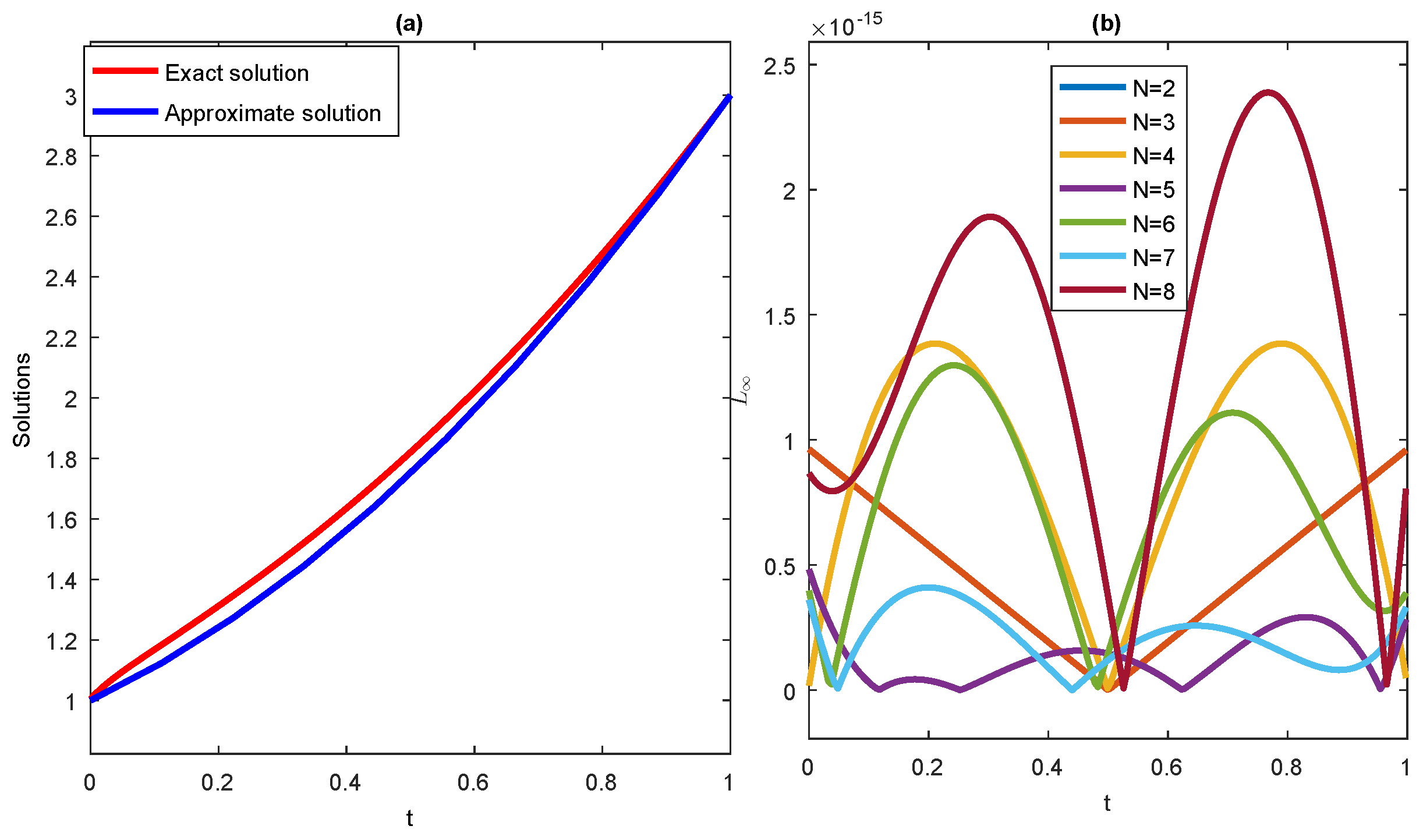
In this section, we apply the algorithms introduced in Section 4, and compare the obtained numerical approximation with the exact solution. In addition, the absolute error $L_{\infty }={\parallel \overline{y}-y\parallel }_{\infty }$ against various scale levels has been presented graphically, where y is the approximate solution and $\overline{y}$ is the exact solution. We used an HP-Cori 5 seventh generation machine, and Matlab 2016 computational software was used for numerical solutions.

Example 1.

Consider the generalized variable-order initial value problem given by

$$\begin{array}{c}\hfill \left\{\begin{array}{c}{D}^{v\left(t\right)}y\left(t\right)+y\left(t\right)=h\left(t\right),t\in [0,1]and0<v\left(t\right)\le 1,\hfill \\ y\left(0\right)=1,\hfill \end{array}\right.\end{array}$$

(47)

where

$$h\left(t\right)=\frac{2t^{2-e^{-t}}}{\Gamma (3-e^{-t})}+\frac{t^{1-e^{-t}}}{\Gamma (2-e^{-t})}+\frac{t^{-e^{-t}}}{\Gamma (1-e^{-t})}+t^2+t+1.$$

At $v\left(t\right)=e^{-t},$ the exact solution of (47) is given by

$$y\left(t\right)=t^2+t+1.$$

We approximate the solution through our proposed numerical scheme. We compare the exact and numerical solution at scale level $N=2$ at the given variable order $v\left(t\right)=e^{-t}$ in Figure 1.

Example 2.

Consider another variable order initial value problem given by

$$\begin{array}{c}\hfill \left\{\begin{array}{c}{D}^{v\left(t\right)}y\left(t\right)+2y\left(t\right)=h\left(t\right),t\in [0,1]and0<v\left(t\right)\le 1\hfill \\ y\left(0\right)=2,\hfill \end{array}\right.\end{array}$$

(48)

where

$$h\left(t\right)=\frac{4t^{2-\left(\frac{t+1}{2}\right)}}{\Gamma (3-\left(\frac{t+1}{2}\right))}-\frac{4t^{1-\left(\frac{t+1}{2}\right)}}{\Gamma (2-\left(\frac{t+1}{2}\right))}+\frac{2t^{-\left(\frac{t+1}{2}\right)}}{\Gamma (1-\left(\frac{t+1}{2}\right))}+4t^2-8t+4.$$

At $v\left(t\right)=\frac{t+1}{2},$ the exact solution of Equation (48) is given by

$$y\left(t\right)=2{(1-t)}^2.$$

We approximate the solution through our proposed numerical scheme. We compare the exact and numerical solution at scale level $N=6$ at the given variable order $v\left(t\right)=\frac{t+1}{2}$ in Figure 2.

Example 3.

Consider the generalized variable order boundary value problem given by

$$\left\{\begin{array}{c}{D}^{v\left(t\right)}y\left(t\right)+D^{v_1\left(t\right)}y\left(t\right)+y\left(t\right)=g\left(t\right),t\in [0,1],1<v\left(t\right)\le 2and0<v_1\left(t\right)\le 1\hfill \\ y\left(0\right)=1,y\left(1\right)=16,\hfill \end{array}\right.$$

(49)

where

$$\begin{array}{cc}& g\left(t\right)=\frac{18t^{2-(e^{-t}+1)}}{\Gamma (3-(e^{-t}+1))}+\frac{6t^{1-(e^{-t}+1)}}{\Gamma (2-(e^{-t}+1))}\hfill \\ & +\frac{t^{-(e^{-t}+1)}}{\Gamma (1-(e^{-t}+1))}+\frac{18t^{2-e^{-t}}}{\Gamma (3-e^{-t})}+\frac{6t^{1-e^{-t}}}{\Gamma (2-e^{-t})}\hfill \\ & +\frac{t^{-e^{-t}}}{\Gamma (1-e^{-t})}+9t^2+6t+1.\hfill \end{array}$$

The exact solution at $v\left(t\right)=e^{-t}+1,$ and at $v_1\left(t\right)=e^{-t}$ of (49), is given by

$$y\left(t\right)=9t^2+6t+1.$$

We approximate the solution through our proposed numerical scheme. We compare the exact and numerical solution at scale level $N=6$ at the given variable order $v\left(t\right)=e^{-t}$ in Figure 3.

Example 4.

Consider another variable-order boundary value problem given by

$$\left\{\begin{array}{c}{D}^{v\left(t\right)}y\left(t\right)+D^{v_1\left(t\right)}y\left(t\right)+\frac{1}{2}y\left(t\right)=g\left(t\right),t\in [0,1],1<v\left(t\right)\le 2,and0<v_1\left(t\right)\le 1,\hfill \\ y\left(0\right)=1,y\left(1\right)=9,\hfill \end{array}\right.$$

(50)

where

$$\begin{array}{cc}& g\left(t\right)=\frac{8t^{2-\left(\frac{t+3}{2}\right)}}{\Gamma (3-\left(\frac{t+3}{2}\right))}+\frac{4t^{1-\left(\frac{t+3}{2}\right)}}{\Gamma (2-\left(\frac{t+3}{2}\right))}\hfill \\ & +\frac{t^{-\left(\frac{t+3}{2}\right)}}{\Gamma (1-\left(\frac{t+3}{2}\right))}+\frac{8t^{2-\left(\frac{t+1}{2}\right)}}{\Gamma (3-\left(\frac{t+1}{2}\right))}+\frac{4t^{1-\left(\frac{t+1}{2}\right)}}{\Gamma (2-\left(\frac{t+1}{2}\right))}+\frac{t^{-\left(\frac{t+1}{2}\right)}}{\Gamma (1-\left(\frac{t+1}{2}\right))}\hfill \\ & +2t^2+2t+\frac{1}{2}.\hfill \end{array}$$

At $v\left(t\right)=\frac{t+3}{2}$ and $v_1\left(t\right)=\frac{t+1}{2},$ the exact solution of (50) is given by

$$y\left(t\right)=4t^2+4t+1.$$

We approximate the solution through our proposed numerical scheme. We compare the exact and numerical solution at scale level $N=16$ at the given variable order $v\left(t\right)=\frac{t+3}{2}$ and $v_1\left(t\right)=\frac{t+1}{2},$ in Figure 4.

6. Conclusions and Discussion

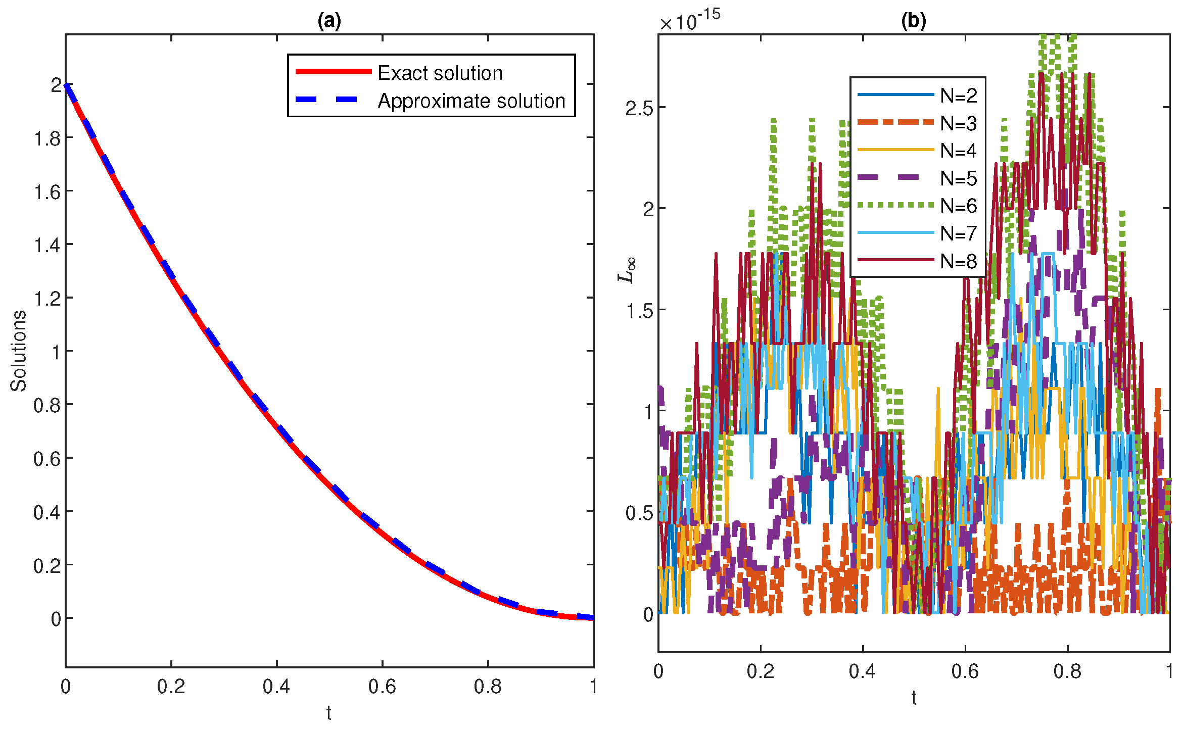
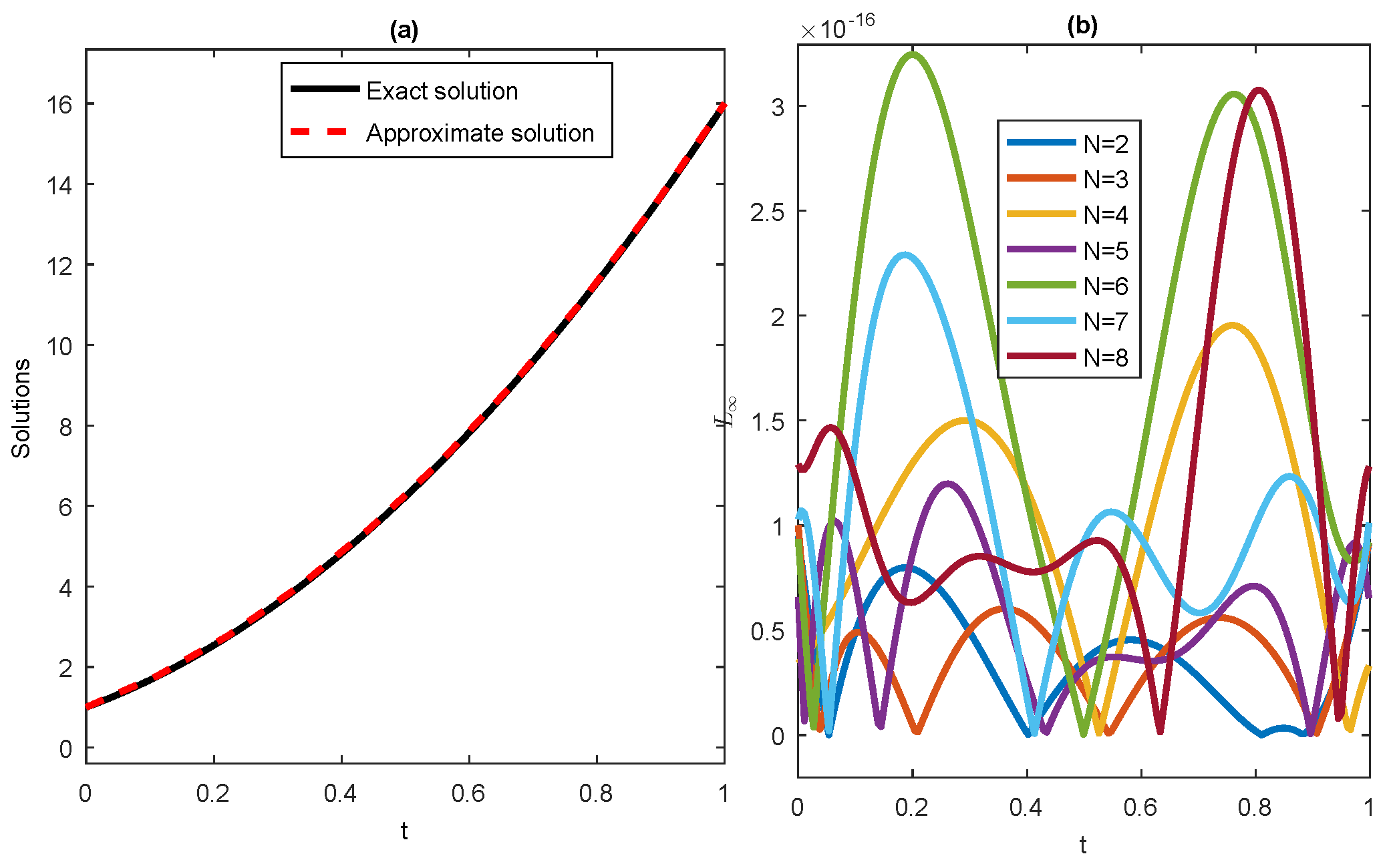
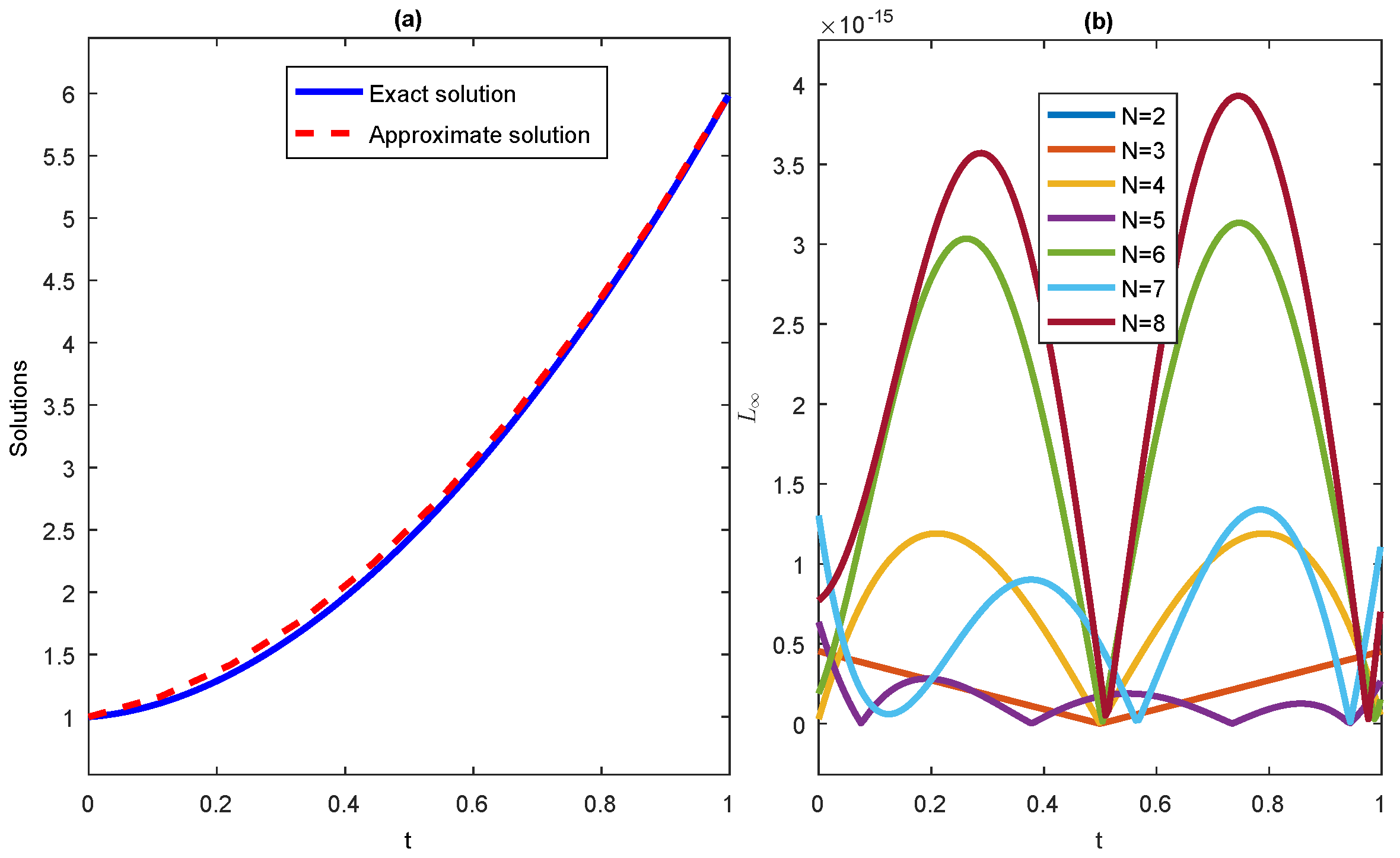
We developed a spectral numerical method for the numerical solutions of VOPs. In this regard, we used Bernoulli polynomials of fractional order to develop different operational matrices corresponding to variable order integration and differentiation. We also developed an operational matrix based on boundary conditions. By utilizing these extended Bernoulli operational matrices, we established numerical algorithms for VOPs, which reduced the given problems to algebraic equations. We solved these equations with the aid of Matlab, and plotted the results graphically. We discussed the convergence of the proposed method in detail. In addition, we applied the method to some problems, to show the efficiency and validity of the method. By comparing the exact and the numerical solutions, we showed that high accuracy can be obtained by increasing the scale level (see Figure 1, Figure 2, Figure 3 and Figure 4). We let y be the approximate solution, and $\overline{y}$ be the exact solution; then, the absolute error $L_{\infty }={\parallel \overline{y}-y\parallel }_{\infty }$ was plotted in the Figure 1, Figure 2, Figure 3 and Figure 4 for different scale levels. From the numerical point of view, it can be said that the proposed method is a powerful spectral method for the numerical investigation of various variable-order differential equations.

References

- Rose, B. Fractional Calculas and Its Applications; Wiley: New York, NY, USA, 1975. [Google Scholar]
- Rossikhin, Y.A.; Shitikova, M.V. Applications of fractional calculas to dynomical problem of linear and nonlinear heridatary mechanics of solids. Appl. Mech. Rev. 1997, 50, 15–67. [Google Scholar] [CrossRef]
- Mainardi, F. Fractional calculas: Some basics problems in continuum and statistical mechanics. In Fractals and Fractional Calculas in Continuum Mechanics; Carpinteri, A., Mainardi, F., Eds.; Springer: New York, NY, USA, 1997; pp. 291–384. [Google Scholar]
- He, J.H. Some applications of nonlinear fractional differential equations and their approximations. Bull. Sci. Technol. 1999, 15, 86–90. [Google Scholar]
- Bagley, R.L.; Torvik, P.J. Fractional calculas in the transient analysis of viscoelastically damped structures. AIAA J. 1985, 23, 918–925. [Google Scholar] [CrossRef]
- Miller, K.S.; Ross, B. An Introduction to the Fractional Calculas and Fractional Differential Equations; Wiley: New York, NY, USA, 1993. [Google Scholar]
- Miller, K.S. Fractional differential equations. J. Fract. Calc. Appl. 1993, 3, 49–57. [Google Scholar]
- Agarwal, R.; Belmekki, M.; Benchohra, M. A survey on similar differential equations and inclusions involving Riemann-Liouville fractional derivative. Adv. Differ. Equ. 2009, 10, 857–868. [Google Scholar]
- Kilbas, A.A.; Trujillo, J.J. Differential equation of fractional order, method, results and problems. Appl. Anal. 2002, 81, 435–493. [Google Scholar] [CrossRef]
- Erturk, V.S.; Momani, S. Solving systems of fractional differential equations using differential transform method. J. Comput. Appl. Math. 2008, 215, 142–151. [Google Scholar] [CrossRef]
- Odibat, Z.; Momani, S. Application of variational iteration method to nonlinear differential equations of fractional order. Int. J. Nonlinear Sci. Numer. Simul. 2006, 1, 15–27. [Google Scholar] [CrossRef]
- Abdulaziz, O.; Hashim, I.; Momani, S. Solving systems of fractional differential equations by homotopy-perturbation method. Phys. Lett. A 2008, 372, 451–459. [Google Scholar] [CrossRef]
- Saadatmandi, A.; Dehghan, M. A tau approach for solution of the space fractional diffusion equation. Comput. Math. Appl. 2011, 62, 1135–1142. [Google Scholar] [CrossRef]
- Saadatmandi, A.; Mohabbati, M. Numerical solution of fractional telegraph equation via the tau method. Math. Rep. 2015, 17, 155–166. [Google Scholar]
- Nemati, S. Numerical solution of Volterra-Fredholm integral equations using Legendre collocation method. J. Comput. Appl. Math. 2015, 278, 29–36. [Google Scholar] [CrossRef]
- Shah, K.; Khalil, H.; Khan, R.A. A generalized scheme based on shifted Jacobi polynomials for numerical simulation of coupled systems of multi-term fractional-order partial differential equations. LMS J. Comput. Math. 2017, 20, 11–29. [Google Scholar] [CrossRef]
- Shah, K.; Jarad, F.; Abdeljawad, T. Stable numerical results to a class of time-space fractional partial differential equations via spectral method. J. Adv. Res. 2020, 25, 39–48. [Google Scholar] [CrossRef] [PubMed]
- Bhrawy, A.H.; Taha, T.M.; Machado, J.A.T. A review of operational matrices and spectral techniques for fractional calculus. Nonlinear Dyn. 2015, 81, 1023–1052. [Google Scholar] [CrossRef]
- Yousefi, S.A.; Behroozifar, M. Operational matrices of Bernstein polynomials and their applications. Int. J. Syst. Sci. 2010, 41, 709–716. [Google Scholar] [CrossRef]
- Samko, S.G.; Rose, B. Integration and differentiation to a variable fractional order. Integral Transform. Spec. Funct. 1993, 1, 277–300. [Google Scholar] [CrossRef]
- Soon, C.M.; Coimbra, F.M.; Kobayashi, M.H. The variable viscoelasticity oscillator. Ann. Phys. 2005, 14, 378–389. [Google Scholar] [CrossRef]
- Lin, R.; Liu, F.; Anh, V.; Turner, I. Stability and convergence of a new explicit finite-difference approximation for the variable-order nonlinear fractional diffusion equation. Appl. Math. Comput. 2009, 212, 435–445. [Google Scholar] [CrossRef]
- Zhuang, P.; Liu, F.; Anh, V.; Turner, I. Numerical methods for the variable-order fractional advanced-diffusion equation with a nonlinear source term. Numer. Anal. 2009, 47, 1760–1781. [Google Scholar] [CrossRef]
- Chen, C.; Liu, F.; Anh, V.; Turner, I. Numerical schemes with high spatial accuracy for a variable-order anamalous subdiffusion equation. Sci. Comput. 2010, 32, 1740–1760. [Google Scholar]
- Amin, R.; Shah, K.; Ahmad, H.; Ganie, A.H.; Abdel-Aty, A.H.; Botmart, T. Haar wavelet method for solution of variable order linear fractional integro-differential equations. AIMS Math. 2022, 7, 5431–5443. [Google Scholar] [CrossRef]
- Bushnaq, S.; Shah, K.; Tahir, S.; Ansari, K.J.; Sarwar, M.; Abdeljawad, T. Computation of numerical solutions to variable order fractional differential equations by using non-orthogonal basis. AIMS Math. 2022, 7, 10917–10938. [Google Scholar] [CrossRef]
- Keshavarz, E.; Ordokhani, Y.; Razzaghi, M. A numerical solution for fractional optimal control problems via Bernoulli polynomials. J. Vib. Control 2016, 22, 3889–3903. [Google Scholar] [CrossRef]
- Sahu, P.K.; Mallick, B. Approximate solution of fractional order Lane-Emden type differential equation by orthonormal Bernoulli’s polynomials. Int. J. Appl. Comput. Math. 2019, 5, 89. [Google Scholar] [CrossRef]
- Behroozifar, M.; Habibi, N. A numerical approach for solving a class of fractional optimal control problems via operational matrix Bernoulli polynomials. J. Vib. Control 2018, 24, 2494–2511. [Google Scholar] [CrossRef]
- Phang, C.; Toh, Y.T.; Nasrudin, F.S.M. An operational matrix method based on poly-Bernoulli polynomials for solving fractional delay differential equations. Computation 2020, 8, 82. [Google Scholar] [CrossRef]
- Yuzbasi, S. Numerical solutions of fractional Riccati type differential equations by means of the Bernstein polynomials. Comput. Appl. Math. 2013, 219, 6328–6343. [Google Scholar]
- El-Gamel, M.; Adel, W.; El-Azab, M.S. Bernoulli polynomial and the numerical solution of high-order boundary value problems. Math. Nat. Sci. 2019, 4, 45–59. [Google Scholar] [CrossRef]
- Kreyszig, E. Introductory Functional Analysis with Applications; Wiley: New York, NY, USA, 1978. [Google Scholar]
- Nemati, S.; Torres, D.F. Application of bernoulli polynomials for solving variable-order fractional optimal control-affine problems. Axioms 2020, 9, 114. [Google Scholar] [CrossRef]
- Atanackovic, T.M.; Stankovic, B. On a differential equation with left and right fractional derivatives. Fract. Calc. Appl. Anal. 2007, 10, 139–150. [Google Scholar] [CrossRef]
- Zaslavsky, G.M. Chaos, fractional kinetics, and anomalous transport. Phys. Rep. 2002, 371, 461–580. [Google Scholar] [CrossRef]
- Metzler, R.; Klafter, J. The random walk’s guide to anomalous diffusion: A fractional dynamics approach. Phys. Rep. 2000, 399, 1–77. [Google Scholar] [CrossRef]
- Pandey, R.K.; Singh, O.P.; Baranwal, V.K. An analytic algorithm for the space-time fractional advection-dispersion equation. Comput. Phys. Commun. 2011, 182, 1134–1144. [Google Scholar] [CrossRef]
- Blaszczyk, T.; Bekus, K.; Szajek, K.; Sumelka, W. Approximation and application of the Riesz-Caputo fractional derivative of variable order with fixed memory. Meccanica 2022, 57, 861–870. [Google Scholar] [CrossRef]
- Pitolli, F.; Sorgentone, C.; Pellegrino, E. Approximation of the Riesz-Caputo derivative by cubic splines. Algorithms 2022, 15, 69. [Google Scholar] [CrossRef]
- Almeida, R.; Tavares, D.; Torres, D.F.M. The Variable-Order Fractional Calculus of Variations; Springer International Publishing: Cham, Switzerland, 2019. [Google Scholar]
- Tohidi, E.; Bhrawy, A.H.; Erfani, K. A collocation method based on Bernoulli operational matrix for numerical solution of generalized pantograph equation. Appl. Math. Model. 2013, 37, 4283–4294. [Google Scholar] [CrossRef]
- Tohidi, E.; Erfani, K.; Gachpazan, M.; Shateyi, S. A new Tau method for solving nonlinear Lane-Emden type equations via Bernoulli operational matrix of differentiation. J. Appl. Math. 2013, 2013, 276585. [Google Scholar] [CrossRef]
Figure 1.
(a) Comparison between exact and numerical solution at for Example 1; (b) Absolute error between exact and numerical solution at various values of N for Example 1.
Figure 2.
(a) Comparison between exact and numerical solution at for Example 2; (b) Absolute error between exact and numerical solution at various values of N of Example 2.
Figure 3.
(a) Comparison between exact and numerical solution at for Example 3; (b) Absolute error between exact and numerical solution at various values of N for Example 3.
Figure 4.
(a) Comparison between exact and numerical solution at for Example 4; (b) Absolute error between exact and numerical solution at various values of N for Example 4.
Disclaimer/Publisher’s Note: The statements, opinions and data contained in all publications are solely those of the individual author(s) and contributor(s) and not of MDPI and/or the editor(s). MDPI and/or the editor(s) disclaim responsibility for any injury to people or property resulting from any ideas, methods, instructions or products referred to in the content. |
© 2023 by the authors. Licensee MDPI, Basel, Switzerland. This article is an open access article distributed under the terms and conditions of the Creative Commons Attribution (CC BY) license (https://creativecommons.org/licenses/by/4.0/).
Share and Cite
MDPI and ACS Style
Khan, Z.A.; Ahmad, S.; Zeb, S.; Alrabaiah, H. Bernoulli-Type Spectral Numerical Scheme for Initial and Boundary Value Problems with Variable Order. Fractal Fract. 2023, 7, 392. https://doi.org/10.3390/fractalfract7050392
AMA Style
Khan ZA, Ahmad S, Zeb S, Alrabaiah H. Bernoulli-Type Spectral Numerical Scheme for Initial and Boundary Value Problems with Variable Order. Fractal and Fractional. 2023; 7(5):392. https://doi.org/10.3390/fractalfract7050392
Chicago/Turabian StyleKhan, Zareen A., Sajjad Ahmad, Salman Zeb, and Hussam Alrabaiah. 2023. "Bernoulli-Type Spectral Numerical Scheme for Initial and Boundary Value Problems with Variable Order" Fractal and Fractional 7, no. 5: 392. https://doi.org/10.3390/fractalfract7050392