Total Value Adjustment of Multi-Asset Derivatives under Multivariate CGMY Processes

Abstract

Counterparty credit risk (CCR) is a significant risk factor that financial institutions have to consider in today’s context, and the COVID-19 pandemic and military conflicts worldwide have heightened concerns about potential default risk. In this work, we investigate the changes in the value of financial derivatives due to counterparty default risk, i.e., total value adjustment (XVA). We perform the XVA for multi-asset option based on the multivariate Carr–Geman–Madan–Yor (CGMY) processes, which can be applied to a wider range of financial derivatives, such as basket options, rainbow options, and index options. For the numerical methods, we use the Monte Carlo method in combination with the alternating direction implicit method (MC-ADI) and the two-dimensional Fourier cosine expansion method (MC-CC) to find the risk exposure and make value adjustments for multi-asset derivatives.

1. Introduction

The concept of value adjustment for financial derivatives started to gain popularity after the financial crisis in 2008. The industry regulations, such as the Basel regulations and the International Financial Reporting Standards (IFRS), are beginning to require the financial institutions to charge the counterparty a premium to balance the credit risk. This premium is often called credit valuation adjustment (CVA), and Ref. [1] gave a very detailed introduction to counterparty credit risk (CCR) and CVA. In the following years, different value adjustments have emerged, which together constitute what is now called total value adjustment (XVA). For the majority of financial derivatives, the most important components of XVA are CVA, FVA, and KVA, where FVA is the funding value adjustment and KVA is the capital value adjustment. For other value adjustments currently in dispute, see, e.g., [2,3].

Currently, there are two approaches to calculate XVA. One is represented by Refs. [4,5,6,7], by constructing a portfolio containing defaultable bonds and deriving the partial differential equation (PDE)/partial integro-differential equation (PIDE). The other method, more commonly used in real markets, is to calculate XVA by estimating the exposure and expected exposure EE. The expected exposures can be seen as potential losses in the future if the counterparty defaults [3], which is related to the value of the derivatives. Based on the numerical estimation of EE, Ref. [8] investigated the CVA and its sensitivities under the Heston model. Ref. [9] proposed a hybrid tree–finite difference method to compute the CVA under the Bates model. Refs. [10,11] and Ref. [12] studied the XVA of the Bermudan option under a pure jump Lévy process. Compared to the diffusion models and the stochastic volatility models, the pure jump Lévy process has better performance to capture all the empirical stylized regularities of stock price movements [13,14]. In this work, we further extend the study in Ref. [12] by expanding the model from one dimension to higher dimensions.

The literature noted above is based on the single-asset model. Let us shift the gaze from a one-dimensional case to a higher-dimensional case. Benefiting from the development of scientific computing, the trading of multi-asset derivatives has expanded in the past decade. For example, the basket option is one illustration of such a derivative. The vanilla option’s essential properties apply to the multivariate product as well, but the underlying option is now a basket of stocks rather than a single stock. It is not simple to price these derivatives, as it requires a model that jointly represents the stock values involved. Similar to the one-dimensional case, value adjustments to multi-asset derivatives are performed based on their exposures. Ref. [15] applied a stochastic grid bundling method to compute the counterparty credit exposure profiles of the multi-asset option, and they prove that this method has high accuracy in the computation of exposure profiles. Ref. [16] considered exponential utility indifference pricing for a multidimensional non-traded assets model subject to inter-temporal default risk. A recent research paper, Ref. [17], used the Gaussian process regression, a machine learning technique, to evaluate the XVA for basket derivatives under the Black–Scholes stochastic model.

Because the exposures are based on the value of derivatives, research on derivative pricing under the multivariate Lévy processes is also of interest. In a review paper, Ref. [18] introduced three main ways to build multivariate Lévy processes: multivariate subordination, affine transformation, and Lévy copulas. The Lévy copulas are not defined on the cumulative distribution function but on the characteristic function of the process. This structure was first simulated and used in option pricing by Ref. [19]. A more commonly used way to build a multivariate Lévy process is affine transformation. It can be seen as a linear combination of Lévy process. Ref. [20] proposed a multivariate risk-neutral Lévy process model by linear combination and presented the model’s applicability in the context of the volatility smile of multiple assets. Ref. [21] proposed a multivariate asset model based on the jump-diffusion process for pricing options written on more than one underlying asset. For the research of multivariate pure jump Lévy processes, Ref. [22] introduced a so-called $\rho \mu$-$VG$ process to capture linear and nonlinear dependence in asset returns.

For the numerical approaches to estimating the value of derivatives with multiple assets, Ref. [23] proposed the primal–dual active set method for solving option values of American better-of option on two assets. Ref. [24] applied a second-order alternating direction implicit (ADI) finite difference method to solve a 2D fractional Black–Scholes equation, where the asset price is based on two independent geometric Lévy processes. Ref. [25] investigated the Crank–Nicolson ADI scheme to approximate the value of the basket option under the Carr–Geman–Madan–Yor (CGMY) process. However, in their paper, the derivation of the fractional partial differential equation (FPDE) associated with the CGMY process is incomplete. In Section 3, we present a detailed derivation of the 2D FPDE based on the multivariate CGMY processes in light of Refs. [25,26,27]. The ADI method enjoys unconditional stability and computational efficiency, which makes it a popular numerical method for solving multi-dimensional problems [28,29,30,31,32,33,34]. Therefore, we here employ the ADI method to find the exposure of a two-asset option. Theoretically, this method can also be extended to higher dimensions, but for the simplicity of numerical calculations, only the two-dimensional case is discussed in this work.

Another popular numerical method to deal with the multi-asset based option is developed by Ref. [35]. They extended the COS method proposed by Ref. [36] to two dimensions, allowing the algorithm to be applied to derivatives such as rainbow options and basket options. In addition, Ref. [37] applied a similar, but modified, sine–sine expansion to numerically calculate the rainbow option. The modified Fourier expansion has an improvement in the approximation of analytical, non-periodic functions. In this work, we will also calculate the multi-asset option exposure using the cosine–cosine expansion method (CC) and compare it to the ADI method.

The rest of this paper is structured as follows. Section 2 reviews some concepts and definitions concerning XVA and the multidimensional Lévy process. In Section 3, we construct two numerical methods, the Monte Carlo method in combination with the alternating direction implicit method (MC-ADI) and the two-dimensional Fourier cosine expansion method (MC-CC), to compute the expected exposure and XVA of the multi-asset option under the multivariate CGMY processes. The numerical results on exposures and XVA are presented in Section 4. Finally, the conclusion and further applications of this work are presented in Section 5.

2. Preliminaries

2.1. The Structure of XVA and Exposure

The classical derivatives valuation, particularly for option pricing, mainly focused on the influence of cash flow. For basic derivative types, the pricing problem was frequently as easy as selecting the appropriate discount factor. The global financial crisis prompted a series of valuation adjustments that took credit risk, funding cost, and regulatory capital cost into account in order to turn a basic valuation into a correct one. A general and simple representation [3] of value adjustments is:

$$\mathrm{Actual}\mathrm{Value}=\mathrm{Base}\mathrm{Value}+\mathit{XVA},$$

where XVA is composed of the various value adjustments, i.e.,

$$\mathit{XVA}=\mathit{CVA}+\mathit{FVA}+\mathit{KVA}.$$

Notice that this expression assumes the XVA component is totally separate from the actual value. This is not completely true in reality, but it can almost always be considered to be a reasonable assumption in practice.

All of the above value adjustments relate to derivatives’ credit exposures. The fact of credit exposure is a positive value of a financial derivative, and the expected exposure $\left(EE\right)$ can be seen as the future value of the derivative. This future exposure gives an indication of the possible loss if a counterparty defaults. Following Ref. [1], let $V\left(t\right)$ be the value of a portfolio at time t, then the exposure $E\left(t\right)$ is defined by

$$E\left(t\right)=V{\left(t\right)}^{+},$$

(1)

where $x^{+}=\max [x,0],$ and the present expected exposure at a future time t is defined by

$$EE\left(t\right)=\mathbb{E}\left[E\left(t\right)\right|{\mathcal{F}}_0],$$

(2)

where ${\mathcal{F}}_0$ is the filtration at time $t=0$. The discounted version of $EE$ is computed as

$$E{E}^{*}\left(t\right)=\mathbb{E}\left[D(0,t)E\left(t\right)\right|{\mathcal{F}}_0],$$

where $D(0,t)$ is the discount factor. We also use potential future exposure (PFE) to represent the best or worst case the buyer may face in the future. It is defined as

$$PF{E}_{\alpha }\left(t\right)=inf\left\{x:\mathbb{P}\left(E\right(t)\le x)\ge \alpha \right\},$$

(3)

where $\alpha$ takes 97.5% and 2.5% in this work.

Then, each part of the XVA is defined as follows.

CVA—The most significant component of XVA is the credit value adjustment, which is also the principal expression for describing the counterparty risk. The CVA can be thought of as the real price of counterparty credit risk, in contrast to traditional credit limitations. According to Ref. [1], assuming independence between default probability ($PD$), exposure, and recovery rate (R), a practical CVA expression is given by

$$\begin{array}{cc}\hfill \mathit{CVA}& =-LGD{\int }_0^{T}E{E}^{*}\left(t\right)dPD\left(t\right)\hfill \\ \hfill & \approx -(1-R)\sum _{m=1}^{M}E{E}^{*}\left(t_m\right)PD(t_{m-1},t_m),\hfill \end{array}$$

(4)

where R is the recovery rate and usually a constant. It is related to loss given default (LGD), and a more detailed definition can be found in Refs. [38,39]. In addition, $\left\{0=t_1<t_2<\right.\left.\dots <t_M=T\right\}$ is a fixed time grid, and $E{E}^{*}$ is the discounted expected exposure. The $PD$ is the default probability. As its name implies, the PD is the probability of counterparty defaults, which is usually derived from credit spreads observed in the market [3]. Let us define the default probability between two sequential times $t_m$ and $t_{m+1}$ as $PD(t_m,t_{m+1})$; a commonly used approximation [3,40] of PD is:

$$\begin{array}{c}\hfill PD(t_m,t_{m+1})\approx \exp \left(-\frac{s\left(t_m\right)·t_m}{LGD}\right)-\exp \left(-\frac{s\left(t_{m+1}\right)·t_{m+1}}{LGD}\right),\end{array}$$

(5)

where $s\left(t\right)$ is the credit spread at time t.

FVA—A large portion of OTC derivatives are traded without collateral due to liquidity and capacity limitations. The funding value adjustment can be generally regarded as a funding cost for these uncollateralized trades, which are a source of funding risk [3,41]. An intuitive FVA formula is:

$$\begin{array}{cc}\hfill FVA& =-{\int }_0^T(EP{E}^{*}\left(t\right)-EN{E}^{*}\left(t\right))·s^f\left(t\right)dt\hfill \\ \hfill & \approx -\sum _{m=1}^M\left(EP{E}^{*}\left(t_m\right)-EN{E}^{*}\left(t_m\right)\right)\hfill \\ \hfill & \times \left\{\exp \left[-s^f\left(t_{m-1}\right)·t_{m-1}\right]-\exp \left[-s^f\left(t_m\right)·t_m\right]\right\},\hfill \end{array}$$

(6)

where $EP{E}^{*}$ and $EN{E}^{*}$ are discounted expected positive exposure and discounted expected negative exposure, respectively, and $s^f\left(t\right)$ is the market funding spread. For a future time t, the $EPE$ and $ENE$ are given by:

$$\begin{array}{cc}\hfill & EPE\left(t\right):=\mathbb{E}\left[E^{+}\left(t\right)\right|{\mathcal{F}}_0],\hfill \\ \hfill & ENE\left(t\right):=\mathbb{E}\left[E^{-}\left(t\right)\right|{\mathcal{F}}_0],\hfill \end{array}$$

(7)

where $x^{-}=\min [x,0]$. In this work, we price options whose option values can never be negative. Therefore, the $ENE:=0$ and the FVA can be simplified to:

$$\mathit{FVA}=-{\int }_0^{T}E{E}^{*}\left(t\right)·s^f\left(t\right)dt.$$

(8)

KVA—In general, the capital value adjustment is a cost incurred by a financial institution to meet regulatory requirements, and it quantifies the tail risk it is exposed to [42]. Regulators set capital use restrictions or require banks to reach a certain capital threshold, at least implicitly charging capital for transactions. The formula of KVA is given by Ref. [3]:

$$\mathit{KVA}=-{\int }_0^{T}E{K}_t·r_c·D{F}_{t}dt,$$

(9)

where $E{K}_t$ is the expected capital, $D{F}_t$ is the survival rate, and $r_c$ is the cost of holding the capital. As we noted in last section, for option pricing, the influence of the KVA can be neglected, thus we will not consider this term when we subsequently calculate XVA.

2.2. Multivariate Lévy Processes and Stock Price Model

Although there are many types of Lévy processes, we can describe them in a concise way using the characteristic function. This is the famous Lévy–Khintchine representation [43,44]:

Lemma 1.

Let ${\left(L_t\right)}_{t\ge 0}$ be a Lévy process on ${\mathbb{R}}^d$ with characteristic triplet $(Q,\gamma ,w)$. Then

$$\mathbb{E}\left[e^{iu.L_t}\right]=e^{t\psi \left(u\right)},u\in {\mathbb{R}}^d$$

with

$$\psi \left(u\right)=-\frac{1}{2}u.Qu+i\gamma .u+{\int }_{{\mathbb{R}}^d}(e^{iu.l}-1-iu.l{\mathbf{1}}_{\left|l\right|\le 1})w\left(dl\right),$$

where $\gamma \in {\mathbb{R}}^d$, $Q\in {\mathbb{R}}^{d\times d}$ is symmetric non-negative definite and w is the Lévy measure.

For real-valued Lévy process, the above formula takes the form:

$$\begin{array}{ccc}& & \mathbb{E}\left[e^{iu{L}_t}\right]=e^{t\psi \left(u\right)},u\in {\mathbb{R}}^d\hfill \\ & & \mathrm{with}\psi \left(u\right)=-\frac{1}{2}{\sigma }^2{u}^2+i\gamma u+{\int }_{-\infty }^{\infty }(e^{iul}-1-iul{\mathbf{1}}_{\left|l\right|\le 1})w\left(dl\right),\hfill \end{array}$$

and $\psi \left(u\right)$ is also known as the characteristic exponent of the Lévy process. A Lévy process is made up of a diffusion component, a drift component, and a jump component. The generating triplet $(Q,\gamma ,w)$ determines these three parts.

Lemma 2.

Let ${\mathbf{X}}_{\mathbf{t}}$ be a pure jump n-dimensional Lévy process (without a Gaussian part) with mutually independent components, and let $\mathbf{A}\in {\mathbb{R}}^{d\times n}$ be a matrix. Then the characteristic exponent of ${\mathbf{Z}}_{\mathbf{t}}={\mathbf{AX}}_{\mathbf{t}}$ is given by

$${\mathsf{\Psi }}_{Z_t}\left(\xi \right)=\sum _{s=1}^n{\mathsf{\Psi }}_{X^s}\left(\sum _{j=1}^d{\xi }_j{\left(A\right)}_{js}\right),$$

(10)

where${\mathsf{\Psi }}_{X^s}$is the characteristic exponent of the marginal $X^s$, and ${\left(A\right)}_{js}$ is the $(j,s)$th entry of the matrix $\mathbf{A}$.

Proof. 

By definition, we have the characteristic function of $Z_t$:

$${\mathsf{\Phi }}_{Z_t}\left(\xi \right)=\mathbb{E}\left[e^{i\xi Z_t}\right]=\mathbb{E}\left[e^{i\xi \left(\mathbf{A}{\mathbf{X}}_{\mathbf{t}}\right)}\right].$$

After rearrangement and using the independence of $X^s$, and noting Lemma 1, we can rewrite:

$$\mathbb{E}\left[e^{i\xi \left(\mathbf{A}{\mathbf{X}}_{\mathbf{t}}\right)}\right]=\prod _{s=1}^n\mathbb{E}\left[e^{i{\sum }_{j=1}^d{\xi }_j{\left(A\right)}_{js}{X}_t^s}\right].$$

By a straightforward calculation and the definition of characteristic component, we can get (10). □

The CGMY process is a typical pure jump process, and the Lévy measure $W\left(dx\right)=w_{CGMY}\left(x\right)$ is defined by [45]

$$w_{CGMY}\left(x\right)=\left\{\begin{array}{cc}C\frac{e^{-Mx}}{x^{1+Y}}\hfill & \mathrm{for}x>0,\hfill \\ C\frac{e^{-G\left|x\right|}}{{\left|x\right|}^{1+Y}}\hfill & \mathrm{for}x<0,\hfill \end{array}\right.$$

(11)

and the characteristic exponent can be obtained through Lévy–Khintchine representation [26]

$${\mathsf{\Psi }}_{CGMY}\left(u\right)=C\mathsf{\Gamma }(-Y)\left[{(M-iu)}^Y-M^Y+{(G+iu)}^Y-G^Y\right],$$

(12)

where $u\in \mathbb{R}$, $\mathsf{\Gamma }(·)$ is a Gamma function, $C>0$, $G\ge 0$, $M\ge 0$, and $Y<2$. The parameter C measures the intensity of jumps. The parameters G and M control the skewness of distribution, which could influence the frequency of large positive jumps and negative jumps. For $Y\in [0,1]$, it means infinite activity processes of finite variation, whereas for $Y\in (1,2)$, the process is infinite activity and infinite variation [46].

According to Lemma 2, we can find the characteristic components of any combination of multivariate pure jump Lévy processes. In this work, for simplicity in numerical calculations, we consider a two-dimensional case for CGMY processes through linear combination without correlation. For two stocks $S_t^1$ and $S_t^2$, the log-return of stocks obeys CGMY processes,

$$\begin{array}{cc}& d\left(\ln S_t^1\right)=(r-{\nu }_1)dt+d{X}_t^1,\end{array}$$

(13)

$$\begin{array}{cc}& d\left(\ln S_t^2\right)=(r-{\nu }_2)dt+d{X}_t^2,\end{array}$$

(14)

with solution

$$\begin{array}{cc}& S_T^1=S_t^1{e}^{(r-{\nu }_1)(T-t)+{\int }_t^{T}d{X}_u^1},\end{array}$$

(15)

$$\begin{array}{cc}& S_T^2=S_t^2{e}^{(r-{\nu }_2)(T-t)+{\int }_t^{T}d{X}_u^2},\end{array}$$

(16)

where $X_t^1$ and $X_t^2$ are two independent CGMY process, r is the risk-free rate, and ${\nu }_1={\mathsf{\Psi }}_{X^1}(-i)$ and ${\nu }_2={\mathsf{\Psi }}_{X^2}(-i)$ are convexity adjustments so that ${\mathbb{E}}^{\mathbb{Q}}\left(S_T\right)=e^{r(T-t)}{S}_t$ under the risk-neutral measure $\mathbb{Q}$. Let

$${\mathbf{Z}}_{\mathbf{t}}={\mathbf{AX}}_{\mathbf{t}}=\left(\begin{array}{cc}{\omega }_1& 0\\ 0& {\omega }_2\end{array}\right)\left(\begin{array}{c}{X}_t^1\\ X_t^2\end{array}\right)$$

(17)

and taking ${\omega }_1={\omega }_2=1$. By Lemma 2, the characteristic component of ${\mathbf{Z}}_{\mathbf{t}}={\mathbf{AX}}_{\mathbf{t}}$ at $t=1$ is

$$\begin{array}{ccc}\hfill \mathsf{\Psi }\left(\xi \right)& & ={\mathsf{\Psi }}_1({\xi }_1{A}_{11}+{\xi }_2{A}_{21})+{\mathsf{\Psi }}_2({\xi }_1{A}_{12}+{\xi }_2{A}_{22})\hfill \\ & & :=\varphi \left(\zeta \right),\hfill \end{array}$$

(18)

where $\xi ={({\xi }_1,{\xi }_2)}^{\mathbf{T}}$ is the dual variable of $x={(x_1,x_2)}^{\mathbf{T}}$ under the Fourier transform, and $\zeta ={({\zeta }_1,{\zeta }_2)}^{\mathbf{T}}$ denotes the dual variable of $z={(z_1,z_2)}^{\mathbf{T}}$.

Remark 1.

The matrix $\mathit{A}$ in (17) can be a general correlation matrix, and the corresponding characteristic component of ${\mathbf{Z}}_{\mathbf{t}}$ is given by Lemma 2. In this work, we simplify the model for subsequent FPDE derivation, the matrix $\mathit{A}$ is diagonal, which means that there is no correlation between $z_1$ and $z_2$.

3. Numerical Method

In this section, we present two numerical methods for calculating XVA for multi-asset derivatives under the multivariate CGMY processes. Both of them are combined with Monte Carlo simulation to obtain the option value and then the value adjustments can be found by the definition in Section 2. Here we have chosen two multi-asset options for numerical experiments, the basket call option as well as the call-on-max rainbow option.

Basket option: Given a vector of weights $\mathit{a}=(a_1,\dots ,a_n)\in {\mathbb{R}}^n$, the basket is defined as the weighted arithmetic average of the n stock prices $S_t^1,\dots ,S_t^n$ at time T:

$${\mathbf{S}}_T=\sum {}_{k=1}^n{a}_k{S}_T^k.$$

Without loss of generality, we assume that $\sum {}_{k=1}^n{a}_k=1$. A basket option in the European style, in which the holder has the right but not the obligation to purchase (or sell) a portfolio of assets with a strike price K only at terminal time T. The payoff function $\phi \left({\mathit{S}}_T\right)$ of the European-style basket option is

$$\phi \left({\mathit{S}}_T\right)=\left\{\begin{array}{cc}{({\mathit{S}}_T-K)}^{+},\hfill & \mathrm{for} \mathrm{a} \mathrm{call} \mathrm{option},\hfill \\ {(K-{\mathit{S}}_T)}^{+},\hfill & \mathrm{for} \mathrm{a} \mathrm{put} \mathrm{option}.\hfill \end{array}\right.$$

(19)

Call-on-max rainbow option: A call-on-max option gives its holder the right to buy the maximum (expensive) asset with the strike price K at maturity. The payoff function of this option is given by

$$\phi ={\left(\max (S_T^1,\dots ,S_T^n)-K\right)}^{+}.$$

(20)

The general steps of the whole algorithm is as follows:

• Simulate paths of underlying price ${\mathbf{S}}_{\mathbf{t}}$ under the multivariate CGMY model by the Monte Carlo method.
• Based on option types, applying the ADI method and cosine–cosine expansion method to find the exposure of each path in step 1.
• Based on the exposure obtained in step 2, CVA, FVA, and XVA are calculated as defined in Section 2.

3.1. Monte Carlo–ADI Method

The Monte Carlo simulation of the CGMY process is based on Refs. [47,48]. It has been proved that the CGMY process can be considered as a time-changed Brownian motion, i.e., the CGMY process can be written as

$$X\left(t\right)=\frac{G-M}{2}\mathrm{Y}\left(t\right)+B\left(\mathrm{Y}\left(t\right)\right),$$

(21)

where $\mathrm{Y}\left(t\right)$ is a subordinator independent of the Brownian motion $B\left(t\right)$. Based on the Laplace transform of this time change subordinator and Rosinski rejection [49], the CGMY process can be simulated by a complex equation containing a confluent hypergeometric function and a parabolic cylinder function. More details about the Monte Carlo simulation of the CGMY process can be found in Ref. [47].

As introduced previously, after obtaining the path of the multivariate CGMY processes by Monte Carlo simulation, a combination of the ADI method needs to be used to obtain the exposure, which is based on the option value. For a two-asset option whose underlying price obeys a binary CGMY process, its value satisfies a 2D FPDE, and below we give the derivation procedure for satisfying the specific conditions and use the ADI method to solve it numerically.

3.1.1. The Derivation of 2D FPDE

Let us start with the definitions of the Riemann–Liouville (RL) tempered fractional derivatives and their Fourier transforms.

Definition 1.

The left and right RL fractional derivatives are given by

$${}_{-\infty }{D}_x^{Y}f\left(x\right)=\frac{1}{\mathsf{\Gamma }(p-Y)}\frac{{\partial }^p}{\partial x^p}{\int }_{-\infty }^x{(x-y)}^{p-Y-1}f\left(y\right)dy,$$

(22)

$${}_x{D}_{\infty }^{Y}f\left(x\right)=\frac{{(-1)}^p}{\mathsf{\Gamma }(p-Y)}\frac{{\partial }^p}{\partial x^p}{\int }_{-\infty }^x{(y-x)}^{p-Y-1}f\left(y\right)dy$$

(23)

for $p-1\le Y<p$, and p is the smallest integer larger than Y. The left and right RL tempered fractional derivatives are

$${}_{-\infty }{D}_x^{Y,G}f:=e^{-Gx}{}_{-\infty }{D}_x^Y\left(e^{Gx}f\right),{}_x{D}_{\infty }^{Y,M}f:=e^{Mx}{}_x{D}_{\infty }^Y\left(e^{-Mx}f\right).$$

The Fourier transform can be shown by a direct calculation.

Lemma 3.

Let $1\le Y<2$, the Fourier transforms of left and right RL tempered fractional derivatives satisfy

$$\mathcal{F}\left({}_{-\infty }{D}_x^{Y,G}f\left(x\right)\right)={(G+i\xi )}^Y\widehat{f}\left(\xi \right),\mathcal{F}\left({}_x{D}_{\infty }^{Y,M}f\left(x\right)\right)={(M-i\xi )}^Y\widehat{f}\left(\xi \right),$$

where $\widehat{f}\left(\xi \right)$ denotes Fourier transform of $f\left(x\right)$.

The value of a two-asset option is given by following theorem.

Theorem 1.

For a two-asset option, if the underlying price is given by $\mathit{Z}$ in (17), then the value of the European-style option satisfies the FPDE

$$\begin{array}{cc}\hfill \frac{\partial V(z,t)}{\partial t}=& (r-{\nu }_1)\frac{\partial V(z,t)}{\partial z_1}+(r-{\nu }_2)\frac{\partial V(z,t)}{\partial z_2}-rV(z,t)\hfill \\ \hfill & +C_1\mathsf{\Gamma }(-Y_1)\left[{}_{-\infty }{D}_{z_1}^{Y_1,G_1}V(z,t)+{}_{z_1}{D}_{\infty }^{Y_1,M_1}V(z,t)-(G_1^{Y_1}+M_1^{Y_1})V(z,t)\right]\hfill \\ \hfill & +C_2\mathsf{\Gamma }(-Y_2)\left[{}_{-\infty }{D}_{z_2}^{Y_2,G_2}V(z,t)+{}_{z_2}{D}_{\infty }^{Y_2,M_2}V(z,t)-(G_2^{Y_2}+M_2^{Y_2})V(z,t)\right],\hfill \end{array}$$

(24)

where ${}_{-\infty }{D}_{z_j}^{Y_j,G_j}$ and ${}_{z_j}{D}_{\infty }^{Y_j,M_j}$, $j=1,2$ are the left and right RL tempered fractional derivatives, and the convexity adjustments $\nu ={\mathsf{\Psi }}_{Z_t}(-i,-i)$.

Proof. 

Writing the value of the option as the risk-neutral expectation of the final payoff $\mathsf{\Pi }(\mathbf{Z},T)$, then

$$V(z,t)=e^{-r(T-t)}{\mathbb{E}}^Q\left[\mathsf{\Pi }(\mathbf{Z},T)\right],$$

(25)

here, $z=\mathit{Ax}$. Assuming the payoff $\mathsf{\Pi }(\mathbf{Z},T)$ has a complex Fourier transform

$$\widehat{\mathsf{\Pi }}(\zeta ,T)={\int }_{-\infty +i{\alpha }_1}^{\infty +i{\alpha }_1}{\int }_{-\infty +i{\alpha }_2}^{\infty +i{\alpha }_2}{e}^{i{\zeta }_1{z}_1+i{\zeta }_2{z}_2}\mathsf{\Pi }(\mathbf{Z},T)d{z}_{1}d{z}_2.$$

(26)

with ${\alpha }_j=\mathrm{Im}{\zeta }_j$, here, $j=1,2$. Then, according to the Fourier inversion theorem, we have

$$\mathsf{\Pi }(\mathbf{Z},T)=\frac{1}{4{\pi }^2}{\int }_{-\infty +i{\alpha }_1}^{\infty +i{\alpha }_1}{\int }_{-\infty +i{\alpha }_2}^{\infty +i{\alpha }_2}{e}^{-i{z}_1{\zeta }_1-i{z}_2{\zeta }_2}\widehat{\mathsf{\Pi }}(\zeta ,T)d{\zeta }_{1}d{\zeta }_2.$$

(27)

Substituting this representation into Equation (25), we have the following equation:

$$\begin{array}{ccc}\hfill V(z,t)& & =\frac{e^{-r(T-t)}}{4{\pi }^2}{\mathbb{E}}^Q\left[{\int }_{-\infty +i{\alpha }_1}^{\infty +i{\alpha }_1}{\int }_{-\infty +i{\alpha }_2}^{\infty +i{\alpha }_2}{e}^{-i{\zeta }_1{z}_1-i{\zeta }_2{z}_2}\widehat{\mathsf{\Pi }}(\zeta ,T)d{\zeta }_{1}d{\zeta }_2\right]\hfill \\ & & =\frac{e^{-r(T-t)}}{4{\pi }^2}{\int }_{-\infty +i{\alpha }_1}^{\infty +i{\alpha }_1}{\int }_{-\infty +i{\alpha }_2}^{\infty +i{\alpha }_2}{\mathbb{E}}^Q\left[e^{-i{\zeta }_1{z}_1-i{\zeta }_2{z}_2}\right]\widehat{\mathsf{\Pi }}(\zeta ,T)d{\zeta }_{1}d{\zeta }_2\hfill \\ & & =\frac{e^{-r(T-t)}}{4{\pi }^2}{\int }_{-\infty +i{\alpha }_1}^{\infty +i{\alpha }_1}{\int }_{-\infty +i{\alpha }_2}^{\infty +i{\alpha }_2}{e}^{-i{\zeta }_1{z}_1-i{\zeta }_2{z}_2+\kappa (T-t)+(T-t)\varphi (-\zeta ))}\widehat{\mathsf{\Pi }}(\zeta ,T)d{\zeta }_{1}d{\zeta }_2,\hfill \end{array}$$

(28)

where $\kappa =-i{\zeta }_1(r-{\nu }_1)-i{\zeta }_2(r-{\nu }_2)$, and $\varphi \left(\zeta \right)$ is the characteristic exponent of the Lévy process $Z_t$. Note that from the Fourier inversion theorem we also have

$$V(z,t)=\frac{1}{4{\pi }^2}{\int }_{-\infty +i{\alpha }_1}^{\infty +i{\alpha }_1}{\int }_{-\infty +i{\alpha }_2}^{\infty +i{\alpha }_2}{e}^{-i{\zeta }_1{z}_1-i{\zeta }_2{z}_2}\widehat{V}(\zeta ,t)d{\zeta }_{1}d{\zeta }_2.$$

(29)

Comparing Equations (28) and (29), we conclude:

$$\widehat{V}(\zeta ,t)=e^{-r(T-t)+\kappa (T-t)+(T-t)\varphi (-\zeta )}\widehat{\mathsf{\Pi }}(\zeta ,T).$$

(30)

This Fourier transform of the value of a European-style option satisfies (12) and (18). We have the function $\widehat{V}(\zeta ,t)$ that solves the following differential equation:

$$\frac{\partial \widehat{V}(\zeta ,t)}{\partial t}=\left[r-\kappa -\varphi (-\zeta )\right]\widehat{V}(\zeta ,t),$$

(31)

with boundary condition $\widehat{V}(\zeta ,T)=\widehat{\mathsf{\Pi }}(\zeta ,T)$. According to Lemma 3, we get the FPDE for the two-asset European-style option with the payoff $\mathsf{\Pi }(\mathbf{Z},T)$:

$$\begin{array}{cc}\hfill \frac{\partial V(z,t)}{\partial t}=& (r-{\nu }_1)\frac{\partial V(z,t)}{\partial z_1}+(r-{\nu }_2)\frac{\partial V(z,t)}{\partial z_2}-rV(z,t)\hfill \\ \hfill & +C_1\mathsf{\Gamma }(-Y_1)\left[{}_{-\infty }{D}_{z_1}^{Y_1,G_1}V(z,t)+{}_{z_1}{D}_{\infty }^{Y_1,M_1}V(z,t)-(G_1^{Y_1}+M_1^{Y_1})V(z,t)\right]\hfill \\ \hfill & +C_2\mathsf{\Gamma }(-Y_2)\left[{}_{-\infty }{D}_{z_2}^{Y_2,G_2}V(z,t)+{}_{z_2}{D}_{\infty }^{Y_2,M_2}V(z,t)-(G_2^{Y_2}+M_2^{Y_2})V(z,t)\right],\hfill \end{array}$$

(32)

where ${}_{-\infty }{D}_{z_j}^{Y_j,G_j}$ and ${}_{z_j}{D}_{\infty }^{Y_j,M_j}$, $j=1,2$ are the left and right RL tempered fractional derivatives, and the convexity adjustments $\nu ={\mathsf{\Phi }}_{Z_t}(-i,-i)$. According to Equation (18), we have

$$\begin{array}{ccc}& & {\nu }_1=C_1\mathsf{\Gamma }(-Y_1)\left[{(M_1-1)}^{Y_1}-M_1^{Y_1}+{(G_1+1)}^{Y_1}-G_1^{Y_1}\right]\hfill \\ & & {\nu }_2=C_2\mathsf{\Gamma }(-Y_2)\left[{(M_2-1)}^{Y_1}-M_2^{Y_2}+{(G_2+1)}^{Y_2}-G_2^{Y_2}\right].\hfill \end{array}$$

 □

Theoretically, the variable $\mathbf{Z}$ in Equation (17) can be extended to more dimensional situationssituations with larger number of dimensions, but the difficulty of calculation will also increase rapidly. In this work, we only do numerical calculations in the two-dimensional case. For simplicity, we will use $X_1$ and $X_2$ below to represent two independent Lévy processes. Let us consider a basket option with two underlying assets $S^1=e^{x_1}$ and $S^2=e^{x_2}$. The payoff and boundary condition is given by the following:

$$\begin{array}{ccc}& & V(x_1,x_2,T)=\max \left(a_1{e}^{x_1}+a_2{e}^{x_2}-K,0\right),\hfill \\ & & \underset{x_1\to -\infty }{lim}V(x_1,x_2,t)=0,\underset{x_1\to \infty }{lim}V(x_1,x_2,t)=a_1{e}^{x_{1max}}+a_2{e}^{x_2}-K{e}^{-r(T-t)},\hfill \\ & & \underset{x_2\to -\infty }{lim}V(x_1,x_2,t)=0,\underset{x_2\to \infty }{lim}V(x_1,x_2,t)=a_1{e}^{x_1}+a_2{e}^{x_{2max}}-K{e}^{-r(T-t)},\hfill \end{array}$$

where K is strike price and satisfies $0<K<\min (e^{x_{1max}}-e^{x_{1min}},e^{x_{2max}}-e^{x_{2min}})$; $a_i$ are weighted parameters.

Similarly, for a call-on-max rainbow option, we have

$$\begin{array}{ccc}& & V(x_1,x_2,T)=\max \left(\max (e^{x_1},e^{x_2})-K,0\right),\hfill \\ & & \underset{x_1\to -\infty }{lim}V(x_1,x_2,t)=0,\underset{x_1\to \infty }{lim}V(x_1,x_2,t)=e^{x_1}-K{e}^{-r(T-t)},\hfill \\ & & \underset{x_2\to -\infty }{lim}V(x_1,x_2,t)=0,\underset{x_2\to \infty }{lim}V(x_1,x_2,t)=e^{x_2}-K{e}^{-r(T-t)}.\hfill \end{array}$$

According to Theorem 1, the values of the above basket option and rainbow option follow Equation (24). In the next step, we will use the ADI method to obtain the numerical solution of Equation (24).

Remark 2.

Equation (24) is obtained when there is no correlation between the underlying assets. If we consider the correlation, the mixed derivative term $\frac{\partial V(z,t)}{\partial z_1\partial z_2}$ may appear in (24). However, the derivation of this differential equation is quite difficult. This is an important issue that we will address in future work.

3.1.2. ADI Method for 2D FPDE

In this subsection, we present the numerical approximation to the FPDE related with CGMY processes in two-dimensional space. Note that the unbounded spatial domain is truncated into a bounded one, i.e., $(x_1,x_2)\in \mathsf{\Omega }=(x_{1L},x_{1R})\times (x_{2L},x_{2R}).$

Next, we employ the ADI method to solve the two-dimensional FPDE related with CGMY processes,

$$\begin{array}{cc}\hfill & rV(x_1,x_2,t)=(r-{\nu }_1)\frac{\partial V(x_1,x_2,t)}{\partial x_1}+(r-{\nu }_2)\frac{\partial V(x_1,x_2,t)}{\partial x_2}-\frac{\partial V(x_1,x_2,t)}{\partial t}\hfill \\ \hfill & +C_1\mathsf{\Gamma }(-Y_1){[}_{x_{1L}}{D}_{x_1}^{Y_1,G_1}V(x_1,x_2,t)+{}_{x_1}{D}_{x_{1R}}^{Y_1,M_1}V(x_1,x_2,t)-(G_1^{Y_1}+M_1^{Y_1})V(x_1,x_2,t)]\hfill \\ \hfill & +C_2\mathsf{\Gamma }(-Y_2){[}_{x_{2L}}{D}_{x_2}^{Y_2,G_2}V(x_1,x_2,t)+{}_{x_2}{D}_{x_{2R}}^{Y_2,M_2}V(x_1,x_2,t)-(G_2^{Y_2}+M_2^{Y_2})V(x_1,x_2,t)],\hfill \end{array}$$

(33)

where $(x_1,x_2,t)\in \mathsf{\Omega }\times (0,T)$ and

$$\begin{array}{ccc}& & {}_{x_{1L}}{D}_{x_1}^{Y_1,G_1}V(x_1,x_2,t)=e^{-G_1{x}_1}{}_{x_{1L}}{D}_{x_1}^{Y_1}\left(e^{G_1{x}_1}V(x_1,x_2,t)\right),\hfill \\ & & {}_{x_1}{D}_{x_{1R}}^{Y_1,M_1}V(x_1,x_2,t)=e^{M_1{x}_1}{}_{x_1}{D}_{x_{1R}}^{Y_1}\left(e^{-M_1{x}_1}V(x_1,x_2,t)\right),\hfill \\ & & {}_{x_{2L}}{D}_{x_2}^{Y_2,G_2}V(x_1,x_2,t)=e^{-G_2{x}_2}{}_{x_{2L}}{D}_{x_2}^{Y_2}\left(e^{G_2{x}_2}V(x_1,x_2,t)\right),\hfill \\ & & {}_{x_2}{D}_{x_{2R}}^{Y_2,M_2}V(x_1,x_2,t)=e^{M_2{x}_2}{}_{x_2}{D}_{x_{2R}}^{Y_2}\left(e^{-M_2{x}_2}V(x_1,x_2,t)\right).\hfill \end{array}$$

The temporal domain is divided into $N_t$ parts by the grid points $t_j=j\tau (0\le j\le N_t),$ where the temporal stepsize $\tau =\frac{T}{N_t}.$ The spatial domain is divided into $N_{x_1}{N}_{x_2}$ parts by the mesh points $x_{1n}=x_{1L}+n{h}_{x_1}(0\le n\le N_{x_1}),x_{2m}=x_{2L}+m{h}_{x_2}(0\le m\le N_{x_2})$, where the spatial stepsize $h_{x_1}=\frac{x_{1R}-x_{1L}}{N_{x_1}},h_{x_2}=\frac{x_{2R}-x_{2L}}{N_{x_2}}.$ For simplicity, we set $N=N_{x_1}=N_{x_2},h=h_{x_1}=h_{x_2}.$ The temporal domain is covered by ${\mathsf{\Omega }}_{\tau }=\left\{t_j\right|0\le j\le N_t\}$, and the spatial domain is covered by ${\mathsf{\Omega }}_h=\left\{(x_{1n},x_{2m})\right|0\le n,m\le N\}$. Let ${\mathcal{V}}_h=\{v|v=\{v_{n,m}^j|0\le j\le N_t,0\le n,m\le N\}\}$ be grid function space defined on ${\mathsf{\Omega }}_{\tau }\times {\mathsf{\Omega }}_h$. For the grid function $v\in {\mathcal{V}}_h,$ we have the following notations:

$$v_{n,m}^{j+\frac{1}{2}}=\frac{v_{n,m}^{j+1}+v_{n,m}^j}{2},{\delta }_t{v}_{n,m}^{j+\frac{1}{2}}=\frac{v_{n,m}^{j+1}-v_{n,m}^j}{\tau },$$

$${\delta }_{x_1}{v}_{n,m}^{j+\frac{1}{2}}=\frac{v_{n+1,m}^{j+\frac{1}{2}}-v_{n-1,m}^{j+\frac{1}{2}}}{2h},{\delta }_{x_2}{v}_{n,m}^{j+\frac{1}{2}}=\frac{v_{n,m+1}^{j+\frac{1}{2}}-v_{n,m-1}^{j+\frac{1}{2}}}{2h},$$

and the tempered, weighted, and shifted Grünwald difference (tempered-WSGD) operators are given by [50]:

$$\begin{array}{ccc}\hfill & & {}_L{\mathfrak{D}}_h^{Y_1,G_1}{v}_{n,m}=\frac{1}{h^{Y_1}}\left[\sum _{l=0}^{n+1}{g}_{l,G_1}^{\left(Y_1\right)}{v}_{n-l+1,m}-{\theta }_1\left(G_1\right)v_{n,m}\right],\hfill \end{array}$$

(34)

$$\begin{array}{ccc}& & {}_R{\mathfrak{D}}_h^{Y_1,M_1}{v}_{n,m}=\frac{1}{h^{Y_1}}\left[\sum _{l=0}^{N-n+1}{g}_{l,M_1}^{\left(Y_1\right)}{v}_{n+l-1,m}-{\theta }_1\left(M_1\right)v_{n,m}\right],\hfill \end{array}$$

(35)

$$\begin{array}{ccc}& & {}_L{\mathfrak{D}}_h^{Y_2,G_2}{v}_{n,m}=\frac{1}{h^{Y_2}}\left[\sum _{l=0}^{n+1}{g}_{l,G_2}^{\left(Y_2\right)}{v}_{n,m-l+1}-{\theta }_2\left(G_2\right)v_{n,m}\right],\hfill \end{array}$$

(36)

$$\begin{array}{ccc}& & {}_R{\mathfrak{D}}_h^{Y_2,M_2}{v}_{n,m}=\frac{1}{h^{Y_2}}\left[\sum _{l=0}^{N-n+1}{g}_{l,M_2}^{\left(Y_2\right)}{v}_{n,m+l-1}-{\theta }_2\left(M_2\right)v_{n,m}\right],\hfill \end{array}$$

(37)

here ($\lambda =G_1,G_2,M_1,$ or $M_2$)

$$\begin{array}{ccc}& & {\theta }_1\left(\lambda \right)=\left({\gamma }_1{e}^{h\lambda }+{\gamma }_2+{\gamma }_3{e}^{-h\lambda }\right){\left(1-e^{-h\lambda }\right)}^{Y_1},\hfill \\ & & {\theta }_2\left(\lambda \right)=\left({\gamma }_1{e}^{h\lambda }+{\gamma }_2+{\gamma }_3{e}^{-h\lambda }\right){\left(1-e^{-h\lambda }\right)}^{Y_2},\hfill \end{array}$$

and the weights are given by ($\mu =Y_1$ or $Y_2$)

$$\begin{array}{c}\hfill \left\{\begin{array}{cc}\hfill & g_{0,\lambda }^{\left(\mu \right)}={\gamma }_1{\omega }_0{e}^{h\lambda },g_{1,\lambda }^{\left(\mu \right)}={\gamma }_1{\omega }_1+{\gamma }_2{\omega }_0,\hfill \\ \hfill & g_{l,\lambda }^{\left(\mu \right)}=\left({\gamma }_1{\omega }_l+{\gamma }_2{\omega }_{l-1}+{\gamma }_3{\omega }_{l-2}\right)e^{-(l-1)h\lambda },l\ge 2,\hfill \\ \hfill & {\omega }_0=1,{\omega }_l=\left(1-\frac{1+\mu }{l}\right){\omega }_{l-1},l\ge 1,\hfill \end{array}\right.\end{array}$$

(38)

and the parameters ${\gamma }_1,{\gamma }_2$ and ${\gamma }_3$ admit the following linear system:

$$\begin{array}{c}\hfill \left\{\begin{array}{cc}\hfill & {\gamma }_1=\frac{\mu }{2}+{\gamma }_3,\hfill \\ \hfill & {\gamma }_2=\frac{2-\mu }{2}-2{\gamma }_3,\hfill \end{array}\right.\end{array}$$

(39)

where ${\gamma }_3$ is the free variable.

First, we approximate the first-order space derivatives by using the second-order central difference operators, and for the tempered fractional order derivatives, we use the second-order tempered-WSGD operators [50]. Second, the Crank–Nicolson scheme is employed to discrete the time derivative. Then, we arrive at

$$\begin{array}{ccc}\hfill & & r{V}_{n,m}^{j+\frac{1}{2}}-(r-{\nu }_1){\delta }_{x_1}{V}_{n,m}^{j+\frac{1}{2}}-(r-{\nu }_2){\delta }_{x_2}{V}_{n,m}^{j+\frac{1}{2}}+{\delta }_t{V}_{n,m}^{j+\frac{1}{2}}\hfill \\ & & -C_1\mathsf{\Gamma }(-Y_1){[}_L{\mathfrak{D}}_h^{Y_1,G_1}{V}_{n,m}^{j+\frac{1}{2}}+{}_R{\mathfrak{D}}_h^{Y_1,M_1}{V}_{n,m}^{j+\frac{1}{2}}]-C_2\mathsf{\Gamma }(-Y_2){[}_L{\mathfrak{D}}_h^{Y_2,G_2}{V}_{n,m}^{j+\frac{1}{2}}+{}_R{\mathfrak{D}}_h^{Y_2,M_2}{V}_{n,m}^{j+\frac{1}{2}}]\hfill \\ & & =R_{n,m}^{j+\frac{1}{2}},0\le j\le N_t-1,1\le n,m\le N-1,\hfill \end{array}$$

(40)

and there exists a constant $C_R$ such that the truncation error

$$|R_{n,m}^{j+\frac{1}{2}}|\le C_R({\tau }^2+h^2).$$

(41)

Let

$$L_{x_1}=(r-{\nu }_1){\delta }_{x_1}+C_1\mathsf{\Gamma }(-Y_1){(}_L{\mathfrak{D}}_h^{Y_1,G_1}{+}_R{\mathfrak{D}}_h^{Y_1,M_1}),$$

$$L_{x_2}=(r-{\nu }_2){\delta }_{x_2}+C_2\mathsf{\Gamma }(-Y_2){(}_L{\mathfrak{D}}_h^{Y_2,G_2}{+}_R{\mathfrak{D}}_h^{Y_2,M_2}).$$

After adding suitable correction terms, Equation (40) can be factored into

$$\begin{array}{ccc}\hfill & & [(1+\frac{r}{2}\tau )\mathcal{I}-\frac{\tau }{2}{L}_{x_1}](1-\frac{\tau }{2}{L}_{x_2})V_{n,m}^{j+1}\hfill \\ & & =[(1-\frac{r}{2}\tau )\mathcal{I}+\frac{\tau }{2}{L}_{x_1}](1+\frac{\tau }{2}{L}_{x_2})V_{n,m}^j+R{1}_{n,m}^{j+\frac{1}{2}},\hfill \end{array}$$

(42)

and there exists a positive constant $C_{R1}$ such that the truncation error $R{1}_{n,m}^{j+\frac{1}{2}}$ satisfies

$$|R{1}_{n,m}^{j+\frac{1}{2}}|\le C_{R1}({\tau }^2+h^2).$$

(43)

Dropping the truncation error $R{1}_{n,m}^{j+\frac{1}{2}}$, and replacing the exact solution $V_{n,m}^{j+\frac{1}{2}}$ with the numerical approximation $v_{n,m}^{j+\frac{1}{2}}$, we have

$$\begin{array}{ccc}\hfill & & [(1+\frac{r}{2}\tau )\mathcal{I}-\frac{\tau }{2}{L}_{x_1}](1-\frac{\tau }{2}{L}_{x_2})v_{n,m}^{j+1}\hfill \\ & & =[(1-\frac{r}{2}\tau )\mathcal{I}+\frac{\tau }{2}{L}_{x_1}](1+\frac{\tau }{2}{L}_{x_2})v_{n,m}^j.\hfill \end{array}$$

(44)

For Equation (44), introducing an intermediate variable

$$v_{n,m}^{*}=(1-\frac{\tau }{2}{L}_{x_2})v_{n,m}^{j+1},$$

we obtain the ADI scheme for solving the two-dimensional FPDE related with CGMY processes (33):

$$\begin{array}{ccc}\hfill & & [(1+\frac{r}{2}\tau )\mathcal{I}-\frac{\tau }{2}{L}_{x_1}]v_{n,m}^{*}=[(1-\frac{r}{2}\tau )\mathcal{I}+\frac{\tau }{2}{L}_{x_1}](1+\frac{\tau }{2}{L}_{x_2})v_{n,m}^j\hfill \\ & & (1-\frac{\tau }{2}{L}_{x_2})v_{n,m}^{j+1}=v_{n,m}^{*}.\hfill \end{array}$$

(45)

3.1.3. Convergence Test

In this subsection, we carry out a numerical experiment to validate the convergence of the proposed ADI scheme (45).

We consider the following two-dimensional FPDE:

$$\begin{array}{ccc}\hfill V(x_1,x_2,t)& =& \frac{\partial V(x_1,x_2,t)}{\partial x_1}+\frac{\partial V(x_1,x_2,t)}{\partial x_2}-\frac{\partial V(x_1,x_2,t)}{\partial t}\hfill \\ & & {+}_0{D}_{x_1}^{Y_1,G_1}V(x_1,x_2,t)V(x_1,x_2,t)-G_1^{Y_1}V(x_1,x_2,t)\hfill \\ & & {+}_0{D}_{x_2}^{Y_2,G_2}V(x_1,x_2,t)V(x_1,x_2,t)-G_2^{Y_2}V(x_1,x_2,t)]+f(x_1,x_2,t),\hfill \\ & & (x_1,x_2,t)\in {(0,1)}^2\times (0,T).\hfill \end{array}$$

Take the exact solution to be $V(x_1,x_2,t)=e^{-x_1-x_2+t}(x_1^2-x_1^3)(x_2^2-x_2^3)$, and set the parameters $T=1,Y_1=Y_2=1.5,G_1=G_2=1$. The initial and boundary conditions are determined by the exact solution, and the added term $f(x_1,x_2,t)$ is of the following form:

$$\begin{array}{ccc}& & f(x_1,x_2,t)=4e^{-x_1-x_2+t}(x_1^2-x_1^3)(x_2^2-x_2^3)\hfill \\ & & -(x_2^2-x_2^3)e^{-x_1-x_2+t}\left[(2x_1-4x_1^2+x_1^3)+\frac{\mathsf{\Gamma }\left(3\right)}{\mathsf{\Gamma }(3-Y_1)}{x}_1^{2-Y_1}-\frac{\mathsf{\Gamma }\left(4\right)}{\mathsf{\Gamma }(4-Y_1)}{x}_1^{3-Y_1}\right]\hfill \\ & & -(x_1^2-x_1^3)e^{-x_1-x_2+t}\left[(2x_2-4x_2^2+x_2^3)+\frac{\mathsf{\Gamma }\left(3\right)}{\mathsf{\Gamma }(3-Y_2)}{x}_2^{2-Y_2}-\frac{\mathsf{\Gamma }\left(4\right)}{\mathsf{\Gamma }(4-Y_2)}{x}_2^{3-Y_2}\right].\hfill \end{array}$$

The numerical errors and convergence orders are shown in

Table 1. Numerical errors and convergence orders of the ADI scheme.

$\mathit{h}=\mathit{\tau }$	$\parallel {\mathit{V}}_{\mathit{T}}-{\mathit{v}}_{\mathit{T}}{\parallel }_2$	Order	$\parallel {\mathit{V}}_{\mathit{T}}-{\mathit{v}}_{\mathit{T}}{\parallel }_{\mathit{\infty }}$	Order
$\frac{1}{10}$	3.5624 $\times {10}^{-4}$	—	8.6670 $\times {10}^{-4}$	—
$\frac{1}{20}$	8.9622 $\times {10}^{-5}$	1.9909	2.0971 $\times {10}^{-4}$	2.0471
$\frac{1}{40}$	2.2375 $\times {10}^{-5}$	2.0020	5.1710 $\times {10}^{-5}$	2.0199
$\frac{1}{80}$	5.5945 $\times {10}^{-6}$	1.9998	1.2809 $\times {10}^{-5}$	2.0133

. It is observed that the proposed ADI scheme has second-order accuracy in time and space.

3.2. Monte Carlo–Cosine-Cosine Expansion Method

Similar to Section 3.1, when we have the Monte Carlo simulation results, we combine it with 2D Fourier series expansions method to obtain the exposure of derivatives. There are many different types of 2D Fourier series expansions. Ref. [35] pointed out that the cosine–cosine expansion seems to have a better performance in estimating call option. As the examples we gave are all call options, we will use cosine–cosine expansion in this work.

3.2.1. The Cosine–Cosine Expansion of Derivative Value

Let $(\mathsf{\Omega },\mathcal{F},\mathbb{P})$ be a probability space, and let $\mathbb{F}=\left\{{\mathcal{F}}_t\right\}$ be a filtration satisfying the usual conditions. The process ${\mathbf{X}}_{\mathbf{t}}=(X_t^1,X_t^2)$ denotes a 2D stochastic process on the filtered probability space $(\mathsf{\Omega },\mathcal{F},\mathbb{F},\mathbb{P})$, which can be seen as the log-asset prices. Let $T>0$ be the terminal time. The value of a European-style two-asset option $V(t_0;x_1,x_2)$, with payoff $g(X_T^1,X_T^2)$, is given by the risk-neutral option valuation formula

$$\begin{array}{ccc}\hfill V(t_0;x_1,x_2)& & =e^{-r\Delta t}{\mathbb{E}}^{\mathbb{Q}}\left[g(X_T^1,X_T^2)\right|(X_t^1,X_t^2)=(x_1,x_2)]\hfill \\ & & =e^{-r\Delta t}\int {\int }_{{\mathbb{R}}^2}g(y_1,y_2)f(y_1,y_2|x_1,x_2)d{y}_{1}d{y}_2,\hfill \end{array}$$

(46)

where $f(y_1,y_2|x_1,x_2)$ is the conditional density function, r is the risk-free rate, and $\Delta t:=T-t_0$ is the time to expiration.

Assuming that the integrand is integrable, for given $\mathbf{x}=(x_1,x_2)$, we can truncate the infinite integration ranges to a finite domain $[a,b]\times [c,d]\subset {\mathbb{R}}^2$ without losing significant accuracy. The analysis of the truncation error can refer to the original work [35] of the COS-COS method. Then, we can get the approximation $V_1$ of the value V:

$$\begin{array}{ccc}\hfill V_1(t_0;x_1,x_2)& & =e^{-r\Delta t}{\int }_a^b{\int }_c^{d}g(y_1,y_2)f(y_1,y_2|x_1,x_2)d{y}_{1}d{y}_2\hfill \\ & & =e^{-r\Delta t}{\int }_a^b{\int }_c^{d}g(y_1,y_2)\sum _n^{+\infty }\sum _m^{+\infty }{\mathcal{A}}_{n,m}\left(\mathbf{x}\right)\hfill \\ & & \cos \left(n\pi \frac{y_1-a}{b-a}\right)\cos \left(m\pi \frac{y_2-c}{d-c}\right)d{y}_{1}d{y}_2,\hfill \end{array}$$

(47)

and the series coefficients ${\mathcal{A}}_{n,m}\left(\mathbf{x}\right)$ are defined by

$${\mathcal{A}}_{n,m}\left(\mathbf{x}\right):=w_{n.m}{\int }_a^b{\int }_c^{d}f(y_1,y_2|x_1,x_2)\cos \left(n\pi \frac{y_1-a}{b-a}\right)\cos \left(m\pi \frac{y_2-c}{d-c}\right)d{y}_{1}d{y}_2.$$

(48)

In this section, we use the following notations: $w_{0,0}=1/(b-a)(d-c),w_{n,0}=w_{0,m}=2/(b-a)(d-c)$, and $w_{n,m}=4/(b-a)(d-c)$, for $n,m\in \mathbb{N}$. Define that

$$G_{n,m}\left(T\right):=w_{n,m}{\int }_a^b{\int }_c^{d}g(y_1,y_2)\cos \left(n\pi \frac{y_1-a}{b-a}\right)\cos \left(m\pi \frac{y_2-c}{d-c}\right)d{y}_{1}d{y}_2.$$

(49)

Then, the approximation $V_2$ of the value V is the truncation of the series summations:

$$V_2(t_0;x_1,x_2)=\frac{1}{w_{n,m}}{e}^{-r\Delta t}\sum _{n=0}^{N-1}\sum _{m=0}^{M-1}{A}_{n,m}\left(\mathbf{x}\right)G_{n,m}\left(T\right).$$

(50)

It has been proved in [35,37] that ${\mathcal{A}}_{n,m}\left(\mathbf{x}\right)$ can be approximated by

$$\begin{array}{cc}\hfill {\mathcal{A}}_{n,m}\left(\mathbf{x}\right)& \approx \frac{w_{n.m}}{2}\left\{\mathrm{Re}\left[\varphi \left(\frac{n\pi }{b-a},\frac{m\pi }{d-c}\mid x_1,x_2\right)\exp \left(-i\frac{n\pi y_1}{b-a}\right)\exp \left(-i\frac{m\pi y_2}{d-c}\right)\right]\right.\\ & \left.+\mathrm{Re}\left[\varphi \left(\frac{n\pi }{b-a},\frac{m\pi }{d-c}\mid x_1,x_2\right)\exp \left(-i\frac{n\pi y_1}{b-a}\right)\exp \left(i\frac{m\pi y_2}{d-c}\right)\right]\right\}.\end{array}$$

(51)

Here, $\mathrm{Re}\{·\}$ denotes the real part of the argument; $\phi (.,.|\mathbf{x})$ is the bivariate conditional characteristic function of given ${\mathbf{X}}_{{\mathbf{t}}_{\mathbf{0}}}=\mathbf{x}$. For a specific Lévy process, we can let ${\varphi }_{levy}(u_1,u_2):=\varphi (u_1,u_2|0,0)$. Inserting Equation (52) into Equation (50), we get the 2D-COS formula for approximation of V:

$$\begin{array}{ccc}\hfill \widehat{V}(t_0;x_1,x_2)=\frac{1}{2}{e}^{-r\Delta t}{\sum _{n=0}^{N-1}}^{\prime }{\sum _{m=0}^{M-1}}^{\prime }& & \left[\mathrm{Re}\left\{{\varphi }_{levy}\left(\frac{n\pi }{b-a},\frac{m\pi }{d-c}\mid x_1,x_2\right)\right.\right.\hfill \\ & & ·\left.\exp \left(-i\frac{n\pi y_1}{b-a}\right)\exp \left(-i\frac{m\pi y_2}{d-c}\right)\right\}\hfill \\ \hfill & & +\mathrm{Re}\left\{{\varphi }_{levy}\left(\frac{n\pi }{b-a},\frac{m\pi }{d-c}\mid x_1,x_2\right)\right.\hfill \\ & & ·\left.\left.\exp \left(-i\frac{n\pi y_1}{b-a}\right)\exp \left(i\frac{m\pi y_2}{d-c}\right)\right\}\right]G_{n,m}\left(T\right).\hfill \end{array}$$

(52)

For different types of derivatives, the payoff-related function $G_{n,m}\left(T\right)$ may or may not have analytical solutions. For the payoff functions (19) and (20), Equation (49) does not have an analytical solution. For this case, we will use the discrete cosine transforms (DCTs) to obtain a numerical solution for $G_{n,m}\left(T\right)$.

3.2.2. The Discrete Cosine Transforms Approximation

In this subsection, we will give a brief introduction of the DCT method. Taking $Q\ge \max [N,M]$ and define

$$\begin{array}{c}\hfill y_1^{q_1}:=a+(q_1+\frac{1}{2})\frac{b-a}{Q}\mathrm{and}\Delta y_1:=\frac{b-a}{Q},\\ \hfill y_2^{q_2}:=c+(q_2+\frac{1}{2})\frac{d-c}{Q}\mathrm{and}\Delta y_2:=\frac{d-c}{Q}.\end{array}$$

The midpoint-rule integration gives us

$$\begin{array}{ccc}\hfill G_{n,m}\left(T\right)& & \approx \sum _{q_1=0}^{Q-1}\sum _{q_2=0}^{Q-1}{\omega }_{n,m}g(y_1^{q_1},y_2^{q_2})\cos \left(n\pi \frac{y_1^{q_1}-a}{b-a}\right)\hfill \\ & & ·\cos \left(m\pi \frac{y_2^{q_2}-c}{d-c}\right)\Delta y_1\Delta y_2\hfill \\ & & =\sum _{q_1=0}^{Q-1}\sum _{q_2=0}^{Q-1}g(y_1^{q_1},y_2^{q_2})\cos \left(n\pi \frac{2q_1+1}{2Q}\right)\cos \left(m\pi \frac{2q_2+1}{2Q}\right)\frac{2}{Q}\frac{2}{Q}.\hfill \end{array}$$

(53)

Inserting Equation (53) into Equation (52) gives us the value of the option. For European-style options, the option value is always positive. When we combine this with the Monte Carlo simulation results, we can get the expected exposure

$$EE(t)=\mathbb{E}[E(t)|{\mathcal{F}}_0]=\mathbb{E}[\widehat{V}(t;x_1,x_2)|{\mathcal{F}}_0].$$

4. Numerical Results and Discussion

In this section, we will present several numerical results for value adjustments of the basket option and rainbow option under the multivariate CGMY processes. The parameters of different cases can be found in

Table 2. Parameter setting for basket options and rainbow options.

		C	G	M	Y	${\mathit{S}}_0$
Basket	Process $X_t^1$	1	5	6	1.5	40
	Process $X_t^2$	1	10	12	1.2	40
Rainbow	Process $X_t^1$	0.5	25	26	1.5	40
	Process $X_t^2$	0.5	20	22	1.2	45

. The risk-free rate $r=0.1$ is not changed in every experiment. The terminal times of the basket option and rainbow option are $T=1$ and $T=0.5$, respectively. For each process $X_t^1$ and process $X_t^2$, we generated 1000 Monte Carlo simulation paths. In all cases, experiments have been performed using MATLAB on an Intel(R) Core(TM) i7-8700 CPU computer.

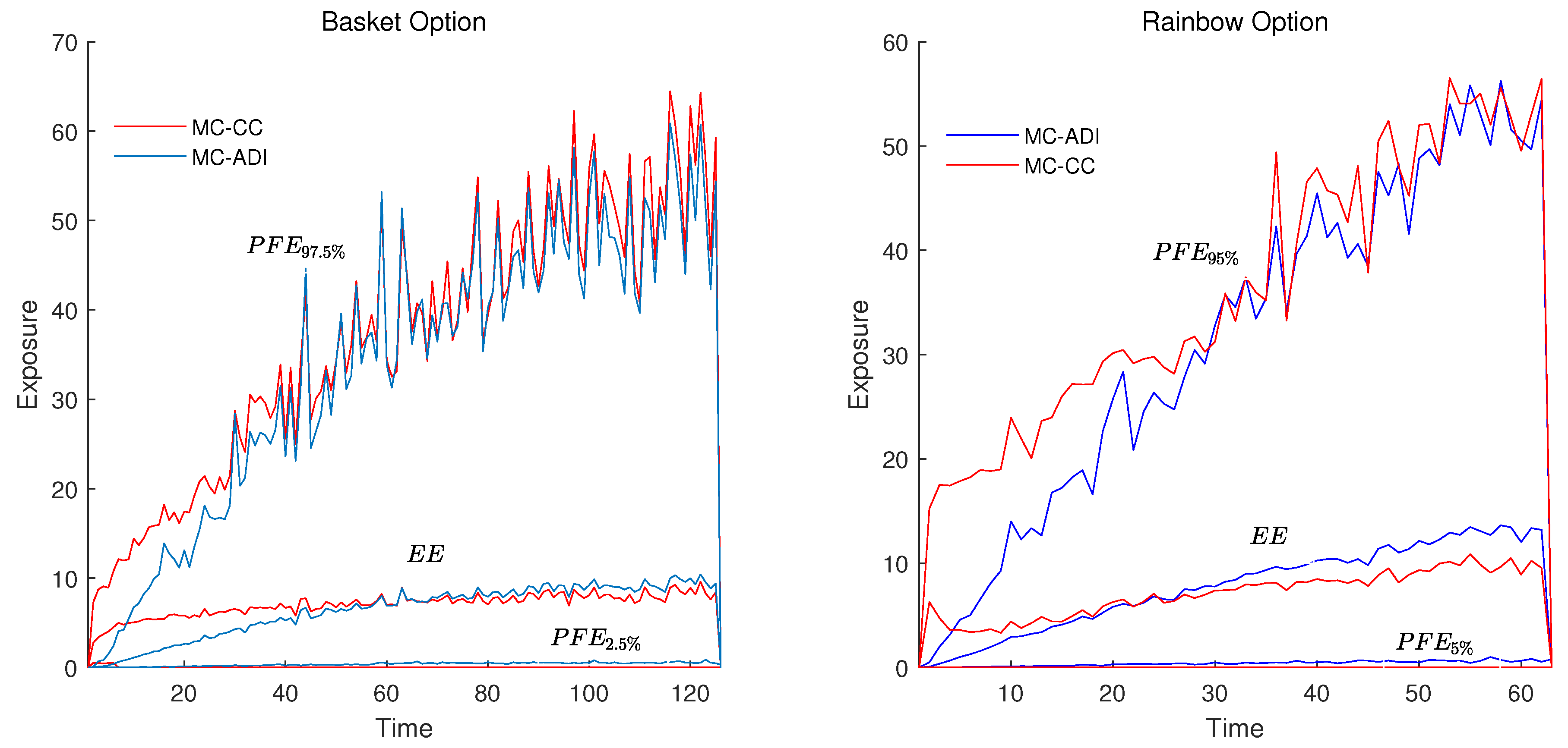
The exposure curve for a multi-asset option is very different from that of single-asset one. For the basket option, in the left graph of Figure 1, it can be seen that the fluctuation of $PF{E}_{97.5\%}$ is very obvious, gradually increasing with time and rapidly decreasing near the terminal time. The right graph of Figure 1 is for a call-on-max rainbow option; the $PF{E}_{97.5\%}$ grows quickly amidst volatility, and its expected exposure $EE$ has been increasing over time in addition to going to zero at maturity. The reason for the exposures going to zero at maturity is because when it expires, we already know whether the option will be exercised or not.

In Figure 1, we can see that the exposure paths obtained by the MC-ADI method and the MC-CC method are quite different, but the overall trend is the same. This is due to the difference between the two methods in calculating values around the strike price, especially in the early days of the option (i.e., around the initial time), where the Monte Carlo simulation prices starting from $S_0$ fluctuates around the strike price. However, when calculating the final results, which are the value adjustments, the difference between their calculations is minor. As can be seen in

Table 3. CVA, FVA, and XVA of Basket Option, comparison and difference of the MC-ADI and MC-CC methods.

	MC-ADI	MC-CC	Difference
CVA	−9.5826%	−10.0421%	0.4595%
FVA	−3.1944%	−3.3514%	0.1570%
XVA	−12.7770%	−13.3935%	0.6165%

and

Table 4. CVA, FVA, and XVA of Rainbow Option, comparison and difference of the MC-ADI and MC-CC methods.

	MC-ADI	MC-CC	Difference
CVA	−11.1571%	−10.6143%	0.5428%
FVA	−3.7185%	−3.5462%	0.1723%
XVA	−14.8753%	−14.1605%	0.7151%

, the rainbow option has a larger XVA. The differences between the CVA, FVA, and XVA obtained by the two methods are quite small.

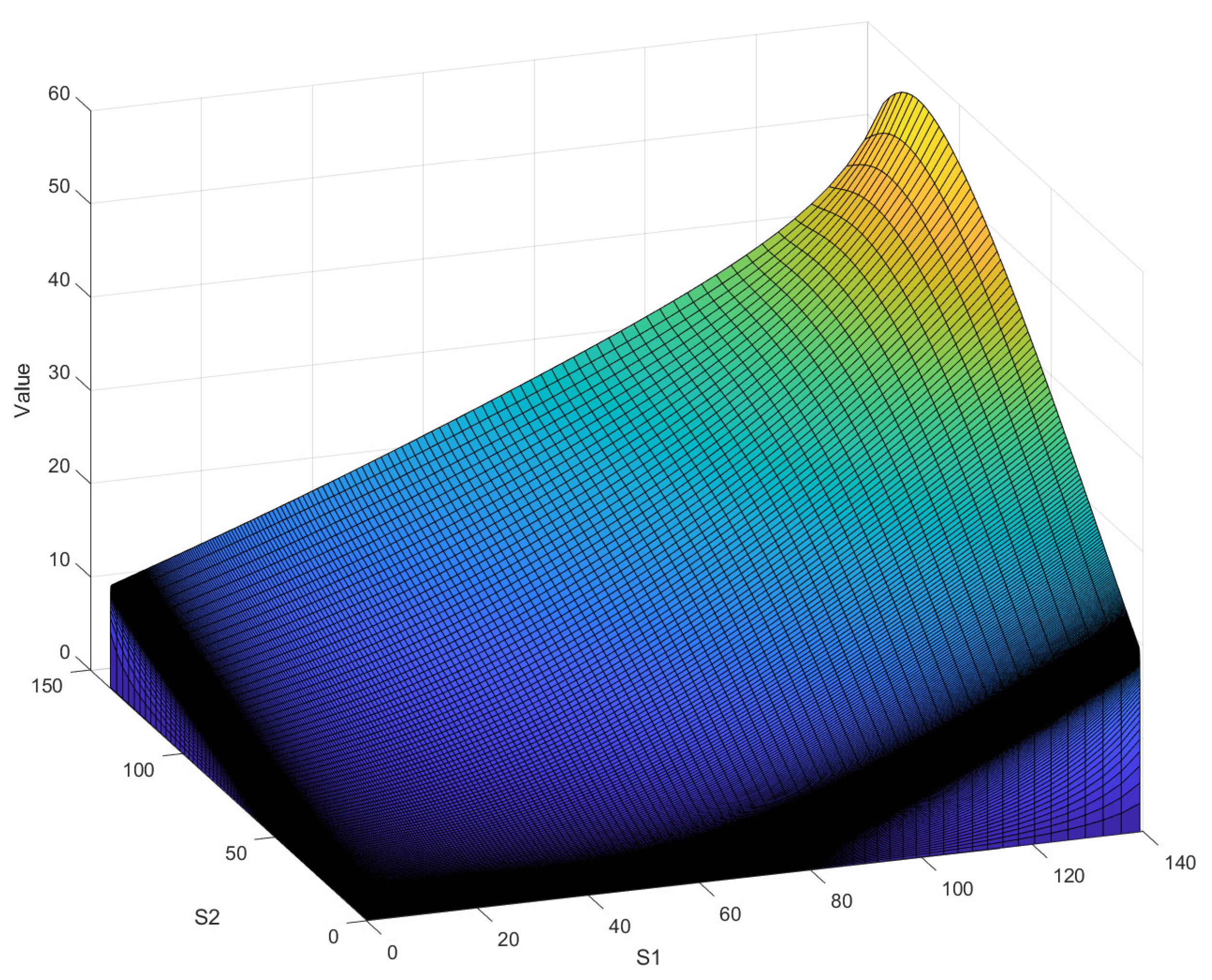
In terms of computational efficiency, the MC-ADI method is more efficient than the MC-CC method.

Table 5. Comparison of the calculation time (in hours) of the two methods.

	MC-ADI	MC-CC
Basket	1.8798	4.6667
Rainbow	1.9943	4.7001

gives the computation time of the two methods in calculating different options, and it can be seen that the MC-CC method takes more than twice the time of the MC-ADI method. This is mainly due to two reasons. First, the MC-CC method needs to use the DCT method to perform the calculation when facing complex boundary conditions, and more computational resources are needed to perform the numerical calculation of the boundaries in order to maintain a high accuracy. The second is that the ADI method can generate a value surface when calculating the option value, as shown in Figure 2. When combined with the Monte Carlo simulation paths, the option values can be quickly located at the corresponding position. For the MC-CC method, on the other hand, one calculation is required at each price node of each simulation path.

In general, although the exposure paths of the two methods are not exactly the same, the final value adjustments obtained are almost the same. The MC-ADI method has a better computational efficiency. Through numerical experiments, we can see that the counterparty default risk can significantly reduce the option value.

5. Conclusions

After several financial crises and rapid changes in financial markets, the impact of counterparty default risk on the value of derivatives is becoming more and more significant. In this work, we focus on the XVA of the multi-asset derivatives. We have used two approaches to find it where underlying assets follow a multivariate CGMY process. The exposures are calculated at each Monte Carlo simulated path in both approaches. Although we have only discussed the CGMY model in this work, the approach is similar for other pure jump Lévy processes. For example, when the CGMY parameter $Y=0$, we can obtain the VG model, and the KoBoL model can also be obtained by making appropriate adjustments to the parameters.

Compared to a single-asset model, the exposures of options under multi-asset conditions fluctuate more. The overall fluctuation trends of the exposures we obtained using the MC-ADI method and the MC-CC method are consistent, but the final calculated XVA has some minor differences. This may be due to the fact that the cosine–cosine expansion method has some errors around the strike price. Similar to the one-dimensional case, the impact of the pure jump feature on exposure is most significant for $PF{E}_{97.5\%}$. Compared to FVA, the effect of CVA on option value is more pronounced. The existence of XVA can significantly reduce the value of the option.

References

- Gregory, J. Counterparty Credit Risk and Credit Value Adjustment: A Continuing Challenge for Global Financial Markets; John Wiley & Sons: Hoboken, NJ, USA, 2012. [Google Scholar]
- Kenyon, C. Completing CVA and liquidity: Firm-level positions and collateralized trades. arXiv 2010, arXiv:1009.3361. [Google Scholar] [CrossRef] [Green Version]
- Gregory, J. The xVA Challenge: Counterparty Credit Risk, Funding, Collateral and Capital; John Wiley & Sons: Hoboken, NJ, USA, 2015. [Google Scholar]
- Burgard, C.; Kjaer, M. Partial differential equation representations of derivatives with bilateral counterparty risk and funding costs. J. Credit Risk 2011, 7, 1–19. [Google Scholar] [CrossRef]
- Arregui, I.; Salvador, B.; Vázquez, C. PDE models and numerical methods for total value adjustment in European and American options with counterparty risk. Appl. Math. Comput. 2017, 308, 31–53. [Google Scholar] [CrossRef]
- Borovykh, A.; Pascucci, A.; Oosterlee, C.W. Efficient computation of various valuation adjustments under local Lévy models. SIAM J. Financ. Math. 2018, 9, 251–273. [Google Scholar] [CrossRef] [Green Version]
- Salvador, B.; Oosterlee, C.W. Total value adjustment for a stochastic volatility model. A comparison with the Black–Scholes model. Appl. Math. Comput. 2020, 391, 125489. [Google Scholar] [CrossRef]
- de Graaf, C.; Kandhai, D.; Sloot, P. Efficient estimation of sensitivities for counterparty credit risk with the finite difference Monte Carlo method. J. Comput. Financ. 2016, 21, 83–113. [Google Scholar] [CrossRef] [Green Version]
- Goudenège, L.; Molent, A.; Zanette, A. Computing credit valuation adjustment solving coupled PIDEs in the Bates model. Comput. Manag. Sci. 2020, 17, 163–178. [Google Scholar] [CrossRef]
- Arregui, I.; Salvador, B.; Ševčovič, D.; Vázquez, C. Total value adjustment for European options with two stochastic factors. Mathematical model, analysis and numerical simulation. Comput. Math. Appl. 2018, 76, 725–740. [Google Scholar] [CrossRef]
- Arregui, I.; Salvador, B.; Ševčovič, D.; Vázquez, C. PDE models for American options with counterparty risk and two stochastic factors: Mathematical analysis and numerical solution. Comput. Math. Appl. 2020, 79, 1525–1542. [Google Scholar] [CrossRef]
- Yuan, G.; Ding, D.; Duan, J.; Lu, W.; Wu, F. Total value adjustment of Bermudan option valuation under pure jump Lévy fluctuations. Chaos Interdiscip. J. Nonlinear Sci. 2022, 32, 023127. [Google Scholar] [CrossRef]
- Elliott, R.J.; Osakwe, C.J.U. Option pricing for pure jump processes with Markov switching compensators. Financ. Stoch. 2006, 10, 250–275. [Google Scholar] [CrossRef]
- Geman, H. Pure jump Lévy processes for asset price modelling. J. Bank. Financ. 2002, 26, 1297–1316. [Google Scholar] [CrossRef] [Green Version]
- Shen, Y.; Anderluh, J.; Van Der Weide, J. Algorithmic counterparty credit exposure for multi-asset Bermudan options. Int. J. Theor. Appl. Financ. 2015, 18, 1550001. [Google Scholar] [CrossRef]
- Henderson, V.; Liang, G. A multidimensional exponential utility indifference pricing model with applications to counterparty risk. SIAM J. Control Optim. 2016, 54, 690–717. [Google Scholar] [CrossRef] [Green Version]
- Goudenege, L.; Molent, A.; Zanette, A. Computing XVA for American basket derivatives by Machine Learning techniques. arXiv 2022, arXiv:2209.06485. [Google Scholar]
- Deelstra, G.; Petkovic, A. How they can jump together: Multivariate Lévy processes and option pricing. Belg. Actuar. Bull. 2010, 9, 29–42. [Google Scholar]
- Tankov, P. Simulation and option pricing in Lévy copula models. In Mathematical Modelling of Financial Derivatives, IMA Volumes in Mathematics and Applications; Springer: Berlin/Heidelberg, Germany, 2006. [Google Scholar]
- Kawai, R. A multivariate Lévy process model with linear correlation. Quant. Financ. 2009, 9, 597–606. [Google Scholar] [CrossRef]
- Ballotta, L.; Bonfiglioli, E. Multivariate asset models using Lévy processes and applications. Eur. J. Financ. 2016, 22, 1320–1350. [Google Scholar] [CrossRef] [Green Version]
- Marfè, R. A multivariate pure-jump model with multi-factorial dependence structure. Int. J. Theor. Appl. Financ. 2012, 15, 1250028. [Google Scholar] [CrossRef]
- Gao, Y.; Song, H.; Wang, X.; Zhang, K. Primal-dual active set method for pricing American better-of option on two assets. Commun. Nonlinear Sci. Numer. Simul. 2020, 80, 104976. [Google Scholar] [CrossRef]
- Chen, W.; Wang, S. A 2nd-order ADI finite difference method for a 2D fractional Black–Scholes equation governing European two asset option pricing. Math. Comput. Simul. 2020, 171, 279–293. [Google Scholar] [CrossRef]
- Guo, X.; Li, Y.; Wang, H. A high order finite difference method for tempered fractional diffusion equations with applications to the CGMY model. SIAM J. Sci. Comput. 2018, 40, A3322–A3343. [Google Scholar] [CrossRef]
- Cartea, A.; del Castillo-Negrete, D. Fractional diffusion models of option prices in markets with jumps. Phys. A Stat. Mech. Appl. 2007, 374, 749–763. [Google Scholar] [CrossRef] [Green Version]
- Guo, X.; Li, Y.; Wang, H. Tempered fractional diffusion equations for pricing multi-asset options under CGMYe process. Comput. Math. Appl. 2018, 76, 1500–1514. [Google Scholar] [CrossRef]
- Liao, H.L.; Sun, Z.Z. Maximum norm error bounds of ADI and compact ADI methods for solving parabolic equations. Numer. Methods Partial Differ. Equ. Int. J. 2010, 26, 37–60. [Google Scholar] [CrossRef]
- Zhang, Q.; Zhang, C.; Deng, D. Compact alternating direction implicit method to solve two-dimensional nonlinear delay hyperbolic differential equations. Int. J. Comput. Math. 2014, 91, 964–982. [Google Scholar] [CrossRef]
- Wu, F.; Cheng, X.; Li, D.; Duan, J. A two-level linearized compact ADI scheme for two-dimensional nonlinear reaction–diffusion equations. Comput. Math. Appl. 2018, 75, 2835–2850. [Google Scholar] [CrossRef]
- Qin, H.; Wu, F.; Zhang, J.; Mu, C. A linearized compact ADI scheme for semilinear parabolic problems with distributed delay. J. Sci. Comput. 2021, 87, 1–19. [Google Scholar] [CrossRef]
- Qin, H.; Wu, F.; Ding, D. A linearized compact ADI numerical method for the two-dimensional nonlinear delayed Schrödinger equation. Appl. Math. Comput. 2022, 412, 126580. [Google Scholar] [CrossRef]
- Cheng, X.; Duan, J.; Li, D. A novel compact ADI scheme for two-dimensional Riesz space fractional nonlinear reaction–diffusion equations. Appl. Math. Comput. 2019, 346, 452–464. [Google Scholar] [CrossRef]
- Chen, X.; Di, Y.; Duan, J.; Li, D. Linearized compact ADI schemes for nonlinear time-fractional Schrödinger equations. Appl. Math. Lett. 2018, 84, 160–167. [Google Scholar] [CrossRef]
- Ruijter, M.J.; Oosterlee, C.W. Two-dimensional Fourier cosine series expansion method for pricing financial options. SIAM J. Sci. Comput. 2012, 34, B642–B671. [Google Scholar] [CrossRef] [Green Version]
- Fang, F.; Oosterlee, C.W. A novel pricing method for European options based on Fourier-cosine series expansions. SIAM J. Sci. Comput. 2009, 31, 826–848. [Google Scholar] [CrossRef] [Green Version]
- Meng, Q.J.; Ding, D. An efficient pricing method for rainbow options based on two-dimensional modified sine–sine series expansions. Int. J. Comput. Math. 2013, 90, 1096–1113. [Google Scholar] [CrossRef]
- Unal, H.; Madan, D.; Güntay, L. Pricing the risk of recovery in default with absolute priority rule violation. J. Bank. Financ. 2003, 27, 1001–1025. [Google Scholar] [CrossRef]
- Schläfer, T.; Uhrig-Homburg, M. Is recovery risk priced? J. Bank. Financ. 2014, 40, 257–270. [Google Scholar] [CrossRef]
- Hull, J.C. Options, Futures and Other Derivatives; Pearson: London, UK, 2019. [Google Scholar]
- de Graaf, C. Efficient PDE Based Numerical Estimation of Credit and Liquidity Risk Measures for Realistic Derivative Portfolios. Ph.D. Thesis, University of Amsterdam, Amsterdam, The Netherlands, 2016. [Google Scholar]
- Ruiz, I. A Complete XVA Valuation Framework: Why the “law of one price” is dead. IRuiz Consult 2015, 12, 1–23. [Google Scholar]
- Tankov, P. Financial Modelling with Jump Processes; Chapman and Hall/CRC: Boca Raton, FL, USA, 2003. [Google Scholar]
- Duan, J. An Introduction to Stochastic Dynamics; Cambridge University Press: New York, NY, USA, 2015. [Google Scholar]
- Carr, P.; Geman, H.; Madan, D.B.; Yor, M. The fine structure of asset returns: An empirical investigation. J. Bus. 2002, 75, 305–332. [Google Scholar] [CrossRef] [Green Version]
- Oosterlee, C.W.; Grzelak, L.A. Mathematical Modeling and Computation in Finance: With Exercises and Python and Matlab Computer Codes; World Scientific: Singapore, 2019. [Google Scholar]
- Madan, D.; Yor, M. CGMY and Meixner subordinators are absolutely continuous with respect to one sided stable subordinators. arXiv 2006, arXiv:math/0601173. [Google Scholar]
- Sioutis, S.J. Calibration and Filtering of Exponential Lévy Option Pricing Models. arXiv 2017, arXiv:1705.04780. [Google Scholar]
- Rosiński, J. Series representations of Lévy processes from the perspective of point processes. In Lévy Processes; Springer: Berlin/Heidelberg, Germany, 2001; pp. 401–415. [Google Scholar]
- Li, C.; Deng, W. High order schemes for the tempered fractional diffusion equations. Adv. Comput. Math. 2016, 42, 543–572. [Google Scholar] [CrossRef] [Green Version]
Figure 1.
, , and of the basket and rainbow options, comparison of the MC-ADI and MC-CC methods.
Figure 2.
The value surface of basket and rainbow options at time , generated by the ADI method.