Sensitive Demonstration of the Twin-Core Couplers including Kerr Law Non-Linearity via Beta Derivative Evolution

Abstract

To obtain new solitary wave solutions for non-linear directional couplers using optical meta-materials, a new extended direct algebraic technique (EDAT) is used. This model investigates solitary wave propagation inside a fiber. As a result, twin couplers are the subject of this study. Kerr law is the sort of non-linearity addressed there. Because it offers solutions to problems with large tails or infinite fluctuations, the resulting solution set is more generalized than the current solution because it is turned into a fractional-order derivative. Furthermore, the found solutions are fractional solitons with spatial–temporal fractional beta derivative evolution. In intensity-dependent switches, these nonlinear directional couplers also serve as limiters. Non-linearity alters the transmission constants of a system’s modes. The significance of the beta derivative parameter and mathematical approach is demonstrated graphically, with a few of the extracted solutions. A parametric analysis revealed that the fractional beta derivative parameter has a significant impact on the soliton amplitudes. With the aid of the advanced software tools for numerical computations, the categories of semi-dark solitons, singular dark-pitch solitons, single solitons of Type-1 along with 2, intermingled hyperbolically, trigonometric, and rational solitons were established and evaluated. We also discussed sensitivity analysis, which is an inquiry that determines how sensitive our system is. A comparative investigation via different fractional derivatives was also studied in this paper so that one can easily understand the correlation with other fractional derivatives. The findings demonstrate that the approach is simple and efficient and that it yields generalized analytical results. The findings will be extremely beneficial in examining and comprehending physical issues in nonlinear optics, specifically in twin-core couplers with optical metamaterials.

1. Introduction

Light is transmitted from the main fiber through one or more branch fibers using optical nonlinear couplers, which are widely available. This would multiplex two originating bitstreams over to fiber as well as demultiplex a specific bitstream. Likewise, planar semiconductor packages or split-layer independent phase fibers for solitons disseminating in every layer can be used to create certain couplers. Due to their various visible implementations in the construction of optical ranges, including pulse transmission units in optical channels, nonlinear directional couplers (NLDCs) are now gaining interest.

Optical metamaterial (OMM) is a phenomenon, alternatively termed as photonic metamaterials $PMMs$, and is a form of electromagnetic metamaterial that interacts with light at wavelengths ranging from terahertz through infrared to easily visible. The materials have a cellular, periodic pattern. OMMs are differentiated over photonic band gaps or photonic crystal structures by their subwavelength periodicity. The cells are magnitudes bigger than the atom, but considerably smaller than the radiated wavelength, which is on the order of nanometers. Atoms control the response to electric and magnetic forces, and therefore to light, in a typical material. In metamaterials $\left(MMs\right)$, cells act as atoms in a homogeneous material at sizes greater than the cells, resulting in an effective medium model. At high frequencies, some $PMMs$ show magnetism, resulting in significant magnetic coupling. In the optical range, this might result in a negative index of refraction. Cloaking and transformation optics are two potential uses. $MMs$ have a wide range of potential implementations, including optical filters, medical devices, remote aerospace implementations, sensor recognition as well as telecommunications assessing, intelligent solar power management, crowd management, radomes, high-frequency battlefield connectivity, but also lenses for high-gain transmitters, as well as shielding frameworks from earthquakes. $MMs$ can be used to build superlenses. Such a lens might allow imaging underneath the diffraction limit, which is the lowest resolution that ordinary glass lenses can attain.

Admittedly, synthetic materials are used in the practical layout and manufacturing of OMMs. Due to their new revolutionary as well as interesting expectations for empirical industrial implementations particularly in nonlinear optics, $NLDCs$, together with the above $MMs$, have created a modern aspect of both research and analysis. When a soliton pulse is transmitted via a birefringent fiber, for example, energy may be exchanged between pulses propagating in two orthogonal modes. Two orthogonally polarized solitons can collide and continue to propagate at the same group velocity. This effect is known as soliton trapping, and it is vital for understanding optical soliton switching. The speed, power, and phase of the pulse all influence this type of fiber switching. As a result of the above details, optical solitons are formed on the key components of fiber optic transmission through trans-continental, including trans-oceanic, distances [1,2,3]. To cover optical solitons, many theoretical and computational methods have been studied using only conserved and confined physical systems [4,5], for example, explored how optical solitons behaved in birefringent fibers, including Kerr law nonlinearity. The oscillating collisions between the three solitons for a dual-mode fiber coupler system were investigated by Li et al. [6], Mirzazadeh et al. [7] By applying the $\left(\frac{G^{{}^{\prime }}}{G}\right)$ technique and ansatz method, in optical couplers, Banaza [8] showed soliton results. Xiang et al. [9] showed a controllable Raman soliton self-frequency shift in nonlinear $MMs$. Different types of bright, dark, and singular soliton solutions have been based on defining the $OMMs$ in Refs. [10,11,12].

The analysis for optical solitons within $NLDC$ via $OMMs$, where the conservation and also localization occurs in the physical framework, recently piqued the attention of numerous investigators. Such physical processes were observed by Arnous [13]. Solitons in $NLDC$ incorporating $OMMs$ were investigated throughout. The trial function technique is the integration procedure. There are three categories of couplers to contemplate. They are twin-core couplers, multiple-core couplers with nearest neighbors coupling, and multiple-core couplers, including all neighbors coupling. It should be emphasized because for all three categories of such couplers, dark-soliton solutions have been recovered exclusively for the Kerr law nonlinearity. This would be the approach’s shortcoming.

J.V. Guzman [14], using the trial function procedure, determined that there seem to be five categories of nonlinearities examined, which demonstrated light, dark, as well as singular solitons. A few more nonlinearities could not provide dark- or singular-soliton solutions. They are all sophisticated. Furthermore, log-law nonlinearity demonstrated that the components attributable to $MMs$ required to be adjusted to zero regarding integrability. This resulted in a repetition of the outcomes published in 2014 [3]. This study is largely unfinished. There are many concerns that have yet to be addressed. These include conservation laws, fractional temporal evolution, and a variety of time-dependent or stochastic coefficients. The investigation of optical couplers within the existence of perturbation factors is now ongoing. In a nutshell, the findings of this article open the door for more research into optical couplers in the foreseeable future. The research concentrates [15], not just on beta derivative evolution $\left(BDE\right)$, but also on the efficiency of available approaches for obtaining traveling wave solutions to the modeled equations. The findings of this investigation will help to comprehend not just specific characteristics of wave propagation in nonlinear sciences, particularly nonlinear optics, but also future laboratory investigations in which the investigated model equation is relevant. It should also be emphasized that the auxiliary ordinary differential equation method as well as the generalized Riccati method may be used to discover analytical solutions over any other nonlinear evolution problem using $BDE$, although this is outside the purview of any such investigation.

Throughout this research [16], consultants looked at the third-order nonlinear Schrödinger equation, which simulates wave pulse transmission in less than one trillionth of a second. They obtained several precise traveling wave solutions, using the extended modified approach. Nevertheless, there has been such limited research undertaken to explain the interactions of coherent frameworks if nonlocal along with nonconservative physical problems appear with certain frameworks since conventional models are difficult to use to reveal the influence of physical problems that occur over time in dynamical systems [17]. Fractional derivatives (such as conformable derivatives, Caputo derivatives, Riemann–Liouville derivatives, Hadamard derivatives, and so on) are an amphitheater to resolve the challenges for these frameworks at this point. We draw attention to [18] for more information on other fields of use. Fractional calculus has made a lot of progress in the area of solving models for implementations, and it continues to show that it can produce more practical models. For illustration, see [19].

However, the majority of these derivatives do not satisfy a basic calculus theorem. To solve the limitations of the above fractional derivatives, Atangana et al. [20] introduced a new derivative called $\left(BD\right)$ into calculus, which fulfilled all of the calculus’ essential attributes. Such a derivative should be seen as a perfectly natural continuation of the traditional derivative, and therefore a fractional derivative. As a response, using $\left(BDE\right)$, for $OMMs$, nonlinear structural multiple configurations for $NLDCs$ can now be analyzed. As a consequence, for the first instance in this study, analytical outcomes for twin-core couplers $\left(TCCs\right)$ along with Kerr law nonlinearity via $OMMs$ and $BDE$ were reported.

The following is how the paper is organized: A recapitulation of the EDAT algorithm is shown in Section 2. In Section 3, the beta derivative evolution of twin-core couplers is proposed. The traveling wave transform is used to transfer the nonlinear partial differential equation into the nonlinear ordinary differential equation. Solitary wave solutions using the EDAT are found in Section 4. The graphical description of the results is discussed in Section 5. By considering the constant values of the existing parameters, the analytical solutions are graphically illustrated to demonstrate the potentiality of the EDAT with the fractional beta derivative. Section 6 is about the sensitivity analysis that defines how sensitive our system is, which is an assessment. Section 7 deals with the analysis of results and discussions. We analyzed graphs over distinct and discrete intervals for effective illustration based on their physical ranges; corresponding numerical values for parameters were used as part of our experiment to examine the different dynamic behaviors, patterns, and textures of solitary wave solutions. That whole research also looks at a comparative investigation using significantly different fractional derivatives in Section 8. The conclusion of this whole study is discussed in Section 9.

2. Extended Direct Algebraic Technique Recapitulation

This entire section provides a short but detailed history of the current method, the EDAT [21,22,23]. Assume that we provide the following partial nonlinear differential equation for the structure:

$$R(s,s_t,s_x,s_{tt},s_{xx},\dots )=0,$$

(1)

The dependent variable is s, whereas the independent variables are $(t,x)$. The transformation $s(t,x)=S\left(\xi \right)$ might be used to change Equation (1) into other integer-order nonlinear $ODE$.

$$R^{*}(S,S^{{}^{\prime }},S^{{}^{″}},\dots )=0,$$

(2)

prime reflects the derivative of $\xi$. Assume that Equation (2) has outcomes of category,

$$\begin{array}{c}\hfill S\left(\xi \right)=b_0+\sum _{i=1}^N\left[b_i{\left(X\left(\xi \right)\right)}^i\right],\end{array}$$

(3)

where

$$\begin{array}{c}\hfill X^{\prime }\left(\xi \right)=ln\left(\rho \right)\left({\mu }_1+{\nu }_{1}X\left(\xi \right)+{\zeta }_1{X}^2\left(\xi \right)\right),\rho \ne 0,1.\end{array}$$

(4)

Even if ${\mu }_1$, ${\nu }_1$, and ${\zeta }_1$ are in fact constant values and N may be found by comparing nonlinear quantities, the greatest order derivative is included inside Equation (2). The above are generic replies to Equation (4), in the form of the parameters ${\mu }_1$, ${\nu }_1$, and ${\zeta }_1$. Here, ${\Omega }_1=({\nu }_1^2-4{\mu }_1{\zeta }_1)$.

(1): As ${\Omega }_1<0$ and ${\zeta }_1\ne 0,$

$$\begin{array}{c}\hfill X_1\left(\xi \right)=-\frac{{\nu }_1}{2{\zeta }_1}+\frac{\sqrt{-{\Omega }_1}}{2{\zeta }_1}{tan}_{\rho }\left(\frac{\sqrt{-{\Omega }_1}}{2}\xi \right),\end{array}$$

(5)

$$\begin{array}{c}\hfill X_2\left(\xi \right)=-\frac{{\nu }_1}{2{\zeta }_1}-\frac{\sqrt{-{\Omega }_1}}{2{\zeta }_1}{cot}_{\rho }\left(\frac{\sqrt{-{\Omega }_1}}{2}\xi \right),\end{array}$$

(6)

$$\begin{array}{c}\hfill X_3\left(\xi \right)=-\frac{{\nu }_1}{2{\zeta }_1}+\frac{\sqrt{-{\Omega }_1}}{2{\zeta }_1}\left({tan}_{\rho }\left(\sqrt{-\left({\Omega }_1\right)}\xi \right)\pm \sqrt{mn}{sec}_{\rho }\left(\sqrt{-\left({\Omega }_1\right)}\xi \right)\right),\end{array}$$

(7)

$$\begin{array}{c}\hfill X_4\left(\xi \right)=-\frac{{\nu }_1}{2{\zeta }_1}+\frac{\sqrt{-{\Omega }_1}}{2{\zeta }_1}\left({cot}_{\rho }\left(\sqrt{-{\Omega }_1}\xi \right)\pm \sqrt{mn}{csc}_{\rho }\left(\sqrt{-{\Omega }_1}\xi \right)\right),\end{array}$$

(8)

$$\begin{array}{c}\hfill X_5\left(\xi \right)=-\frac{{\nu }_1}{2{\zeta }_1}+\frac{\sqrt{-{\Omega }_1}}{4{\zeta }_1}\left({tan}_{\rho }\left(\frac{\sqrt{-{\Omega }_1}}{4}\xi \right)-{cot}_{\rho }\left(\frac{\sqrt{-{\Omega }_1}}{4}\xi \right)\right).\end{array}$$

(9)

(2): As ${\Omega }_1>0$ and ${\zeta }_1\ne 0,$

$$\begin{array}{c}\hfill X_6\left(\xi \right)=-\frac{{\nu }_1}{2{\zeta }_1}-\frac{\sqrt{{\Omega }_1}}{2{\zeta }_1}{tanh}_{\rho }\left(\frac{\sqrt{{\Omega }_1}}{2}\xi \right),\end{array}$$

(10)

$$\begin{array}{c}\hfill X_7\left(\xi \right)=-\frac{{\nu }_1}{2{\zeta }_1}-\frac{\sqrt{{\Omega }_1}}{2{\zeta }_1}{coth}_{\rho }\left(\frac{\sqrt{{\Omega }_1}}{2}\xi \right),\end{array}$$

(11)

$$\begin{array}{c}\hfill X_8\left(\xi \right)=-\frac{{\nu }_1}{2{\zeta }_1}+\frac{\sqrt{{\Omega }_1}}{2{\zeta }_1}\left(-{tanh}_{\rho }\left(\sqrt{{\Omega }_1}\xi \right)\pm i\sqrt{mn}{sech}_{\rho }\left(\sqrt{{\Omega }_1}\xi \right)\right),\end{array}$$

(12)

$$\begin{array}{c}\hfill X_9\left(\xi \right)=-\frac{{\nu }_1}{2{\zeta }_1}+\frac{\sqrt{{\Omega }_1}}{2{\zeta }_1}\left(-{coth}_{\rho }\left(\sqrt{{\Omega }_1}\xi \right)\pm \sqrt{mn}{csch}_{\rho }\left(\sqrt{{\Omega }_1}\xi \right)\right),\end{array}$$

(13)

$$\begin{array}{c}\hfill X_{10}\left(\xi \right)=-\frac{{\nu }_1}{2{\zeta }_1}-\frac{\sqrt{{\Omega }_1}}{4{\zeta }_1}\left({tanh}_{\rho }\left(\frac{\sqrt{{\Omega }_1}}{4}\xi \right)+{coth}_{\rho }\left(\frac{\sqrt{{\Omega }_1}}{4}\xi \right)\right).\end{array}$$

(14)

(3): As ${\mu }_1{\zeta }_1>0$ and ${\nu }_1=0,$

$$\begin{array}{c}\hfill X_{11}\left(\xi \right)=\sqrt{\frac{{\mu }_1}{{\zeta }_1}}{tan}_{\rho }\left(\sqrt{{\mu }_1{\zeta }_1}\xi \right),\end{array}$$

(15)

$$\begin{array}{c}\hfill X_{12}\left(\xi \right)=-\sqrt{\frac{{\mu }_1}{{\zeta }_1}}{cot}_{\rho }\left(\sqrt{{\mu }_1{\zeta }_1}\xi \right),\end{array}$$

(16)

$$\begin{array}{c}\hfill X_{13}\left(\xi \right)=\sqrt{\frac{{\mu }_1}{{\zeta }_1}}\left({tan}_{\rho }\left(2\sqrt{{\mu }_1{\zeta }_1}\xi \right)\pm \sqrt{mn}{sec}_{\rho }\left(2\sqrt{{\mu }_1{\zeta }_1}\xi \right)\right),\end{array}$$

(17)

$$\begin{array}{c}\hfill X_{14}\left(\xi \right)=\sqrt{\frac{{\mu }_1}{{\zeta }_1}}\left(-{cot}_{\rho }\left(2\sqrt{{\mu }_1{\zeta }_1}\xi \right)\pm \sqrt{mn}{csc}_{\rho }\left(2\sqrt{{\mu }_1{\zeta }_1}\xi \right)\right),\end{array}$$

(18)

$$\begin{array}{c}\hfill X_{15}\left(\xi \right)=\frac{1}{2}\sqrt{\frac{{\mu }_1}{{\zeta }_1}}\left({tan}_{\rho }\left(\frac{\sqrt{{\mu }_1{\zeta }_1}}{2}\xi \right)-{cot}_{\rho }\left(\frac{\sqrt{{\mu }_1{\zeta }_1}}{2}\xi \right)\right).\end{array}$$

(19)

(4): As ${\mu }_1{\zeta }_1<0$ and ${\nu }_1=0,$

$$\begin{array}{c}\hfill X_{16}\left(\xi \right)=-\sqrt{-\frac{{\mu }_1}{{\zeta }_1}}{tanh}_{\rho }\left(\sqrt{-{\mu }_1{\zeta }_1}\xi \right),\end{array}$$

(20)

$$\begin{array}{c}\hfill X_{17}\left(\xi \right)=-\sqrt{-\frac{{\mu }_1}{{\zeta }_1}}{coth}_{\rho }\left(\sqrt{-{\mu }_1{\zeta }_1}\xi \right),\end{array}$$

(21)

$$\begin{array}{c}\hfill X_{18}\left(\xi \right)=\sqrt{-\frac{{\mu }_1}{{\zeta }_1}}\left(-{tanh}_{\rho }\left(2\sqrt{-{\mu }_1{\zeta }_1}\xi \right)\pm i\sqrt{mn}{sech}_{\rho }\left(2\sqrt{-{\mu }_1{\zeta }_1}\xi \right)\right),\end{array}$$

(22)

$$\begin{array}{c}\hfill X_{19}\left(\xi \right)=\sqrt{-\frac{{\mu }_1}{{\zeta }_1}}\left(-{coth}_{\rho }\left(2\sqrt{-{\mu }_1{\zeta }_1}\xi \right)\pm \sqrt{mn}{csch}_{\rho }\left(2\sqrt{-{\mu }_1{\zeta }_1}\xi \right)\right),\end{array}$$

(23)

$$\begin{array}{c}\hfill X_{20}\left(\xi \right)=-\frac{1}{2}\sqrt{-\frac{{\mu }_1}{{\zeta }_1}}\left({tanh}_{\rho }\left(\frac{\sqrt{-{\mu }_1{\zeta }_1}}{2}\xi \right)+{coth}_{\rho }\left(\frac{\sqrt{-{\mu }_1{\zeta }_1}}{2}\xi \right)\right).\end{array}$$

(24)

(5): As ${\nu }_1=0$ and ${\mu }_1={\zeta }_1,$

$$\begin{array}{c}\hfill X_{21}\left(\xi \right)={tan}_{\rho }\left({\mu }_1\xi \right),\end{array}$$

(25)

$$\begin{array}{c}\hfill X_{22}\left(\xi \right)=-{cot}_{\rho }\left({\mu }_1\xi \right),\end{array}$$

(26)

$$\begin{array}{c}\hfill X_{23}\left(\xi \right)={tan}_{\rho }\left(2{\mu }_1\xi \right)\pm \sqrt{mn}{sec}_{\rho }\left(2{\mu }_1\xi \right),\end{array}$$

(27)

$$X_{24}\left(\xi \right)=-{cot}_{\rho }\left(2{\mu }_1\xi \right)\pm \sqrt{mn}{csc}_{\rho }\left(2{\mu }_1\xi \right),$$

(28)

$$\begin{array}{c}\hfill X_{25}\left(\xi \right)=\frac{1}{2}\left({tan}_{\rho }\left(\frac{{\mu }_1}{2}\xi \right)-{cot}_{\rho }\left(\frac{{\mu }_1}{2}\xi \right)\right).\end{array}$$

(29)

(6): As ${\nu }_1=0$ and ${\zeta }_1=-{\mu }_1,$

$$\begin{array}{c}\hfill X_{26}\left(\xi \right)=-{tanh}_{\rho }\left({\mu }_1\xi \right),\end{array}$$

(30)

$$\begin{array}{c}\hfill X_{27}\left(\xi \right)=-{coth}_{\rho }\left({\mu }_1\xi \right),\end{array}$$

(31)

$$\begin{array}{c}\hfill X_{28}\left(\xi \right)=-{tanh}_{\rho }\left(2{\mu }_1\xi \right)\pm i\sqrt{mn}{sech}_{\rho }\left(2{\mu }_1\xi \right),\end{array}$$

(32)

$$\begin{array}{c}\hfill X_{29}\left(\xi \right)=-{cot}_{\rho }\left(2{\mu }_1\xi \right)\pm \sqrt{mn}{csch}_{\rho }\left(2{\mu }_1\xi \right),\end{array}$$

(33)

$$\begin{array}{c}\hfill X_{30}\left(\xi \right)=-\frac{1}{2}\left({tanh}_{\rho }\left(\frac{{\mu }_1}{2}\xi \right)+{coth}_{\rho }\left(\frac{{\mu }_1}{2}\xi \right)\right).\end{array}$$

(34)

(7): As ${\nu }_1^2=4{\mu }_1{\zeta }_1$,

$$\begin{array}{c}\hfill X_{31}\left(\xi \right)=\frac{-2{\mu }_1({\nu }_1\xi ln\rho +2)}{{\nu }_1^2\xi ln\rho }.\end{array}$$

(35)

(8): As ${\nu }_1=p,{\mu }_1=pq,(q\ne 0)$ and ${\zeta }_1=0$,

$$\begin{array}{c}\hfill X_{32}\left(\xi \right)={\rho }^{p\xi }-q.\end{array}$$

(36)

(9): As ${\nu }_1={\zeta }_1=0$,

$$\begin{array}{c}\hfill X_{33}\left(\xi \right)={\mu }_1\xi ln\rho .\end{array}$$

(37)

(10): As ${\nu }_1={\mu }_1=0$,

$$\begin{array}{c}\hfill X_{34}\left(\xi \right)=\frac{-1}{{\zeta }_1\xi ln\rho }.\end{array}$$

(38)

(11): As ${\mu }_1=0$ and ${\nu }_1\ne 0$,

$$\begin{array}{c}\hfill X_{35}\left(\xi \right)=-\frac{m{\nu }_1}{{\zeta }_1\left({cosh}_{\rho }\left({\nu }_1\xi \right)-{sinh}_{\rho }\left({\nu }_1\xi \right)+m\right)},\end{array}$$

(39)

$$\begin{array}{c}\hfill X_{36}\left(\xi \right)=-\frac{{\nu }_1\left({sinh}_{\rho }\left({\nu }_1\xi \right)+{cosh}_{\rho }\left({\nu }_1\xi \right)\right)}{{\zeta }_1\left({sinh}_{\rho }\left({\nu }_1\xi \right)+{cosh}_{\rho }\left({\nu }_1\xi \right)+n\right)}.\end{array}$$

(40)

(12): As ${\nu }_1=p,{\zeta }_1=pq,(q\ne 0$ and ${\mu }_1=0)$,

$$\begin{array}{c}\hfill X_{37}\left(\xi \right)=-\frac{m{\rho }^{p\xi }}{m-qn{\rho }^{p\xi }}.\end{array}$$

(41)

$$\begin{array}{c}\hfill {sinh}_{\rho }\left(\xi \right)=\frac{m{\rho }^{\xi }-n{\rho }^{-\xi }}{2},{cosh}_{\rho }\left(\xi \right)=\frac{m{\rho }^{\xi }+n{\rho }^{-\xi }}{2},\end{array}$$

$$\begin{array}{c}\hfill {tanh}_{\rho }\left(\xi \right)=\frac{m{\rho }^{\xi }-n{\rho }^{-\xi }}{m{\rho }^{\xi }+n{\rho }^{-\xi }},{coth}_{\rho }\left(\xi \right)=\frac{m{\rho }^{\xi }+n{\rho }^{-\xi }}{m{\rho }^{\xi }-n{\rho }^{-\xi }},\end{array}$$

$$\begin{array}{c}\hfill {sech}_{\rho }\left(\xi \right)=\frac{2}{m{\rho }^{\xi }+n{\rho }^{-\xi }},{csch}_{\rho }\left(\xi \right)=\frac{2}{m{\rho }^{\xi }-n{\rho }^{-\xi }},\end{array}$$

$$\begin{array}{c}\hfill {sin}_{\rho }\left(\xi \right)=\frac{m{\rho }^{i\xi }-n{\rho }^{-i\xi }}{2i},{cos}_{\rho }\left(\xi \right)=\frac{m{\rho }^{i\xi }+n{\rho }^{-i\xi }}{2},\end{array}$$

$$\begin{array}{c}\hfill {tan}_{\rho }\left(\xi \right)=-i\frac{m{\rho }^{i\xi }-n{\rho }^{-i\xi }}{m{\rho }^{i\xi }+n{\rho }^{-i\xi }},{cot}_{\rho }\left(\xi \right)=i\frac{m{\rho }^{i\xi }+n{\rho }^{-i\xi }}{m{\rho }^{i\xi }-n{\rho }^{-i\xi }},\end{array}$$

$$\begin{array}{c}\hfill {sec}_{\rho }\left(\xi \right)=\frac{2}{m{\rho }^{\xi }+n{\rho }^{-\xi }},{csc}_{\rho }\left(\xi \right)=\frac{2i}{m{\rho }^{\xi }-n{\rho }^{-\xi }},\end{array}$$

where m and n are deformation parameters, which are random constants greater than zero.

3. Beta-Derivative Evolution of Twin-Core Couplers

The following scenario is the structure of $\left(TCCs\right)$ through spatial temporal $BD$ evolution, [13,15]:

$$\begin{array}{cc}\hfill {}_0^A{D}_t^{\beta }L+{\alpha }_1{}_0^A{D}_{xx}^{\beta }L+F(\mid L{\mid }^2)L& =l_1{}_0^A{D}_{xx}^{\beta }(\mid L{\mid }^2)L+m_1(\mid L{\mid }^2){}_0^A{D}_{xx}^{\beta }L\\ & +g_1{L}^2{}_0^A{D}_{xx}^{\beta }{L}^{*}+k_{1}M,\end{array}$$

(42)

$$\begin{array}{cc}\hfill {}_0^A{D}_t^{\beta }M+{\alpha }_2{}_0^A{D}_{xx}^{\beta }M+F(\mid M{\mid }^2)M& =l_2{}_0^A{D}_{xx}^{\beta }(\mid M{\mid }^2)M+m_2(\mid M{\mid }^2){}_0^A{D}_{xx}^{\beta }M\\ & +g_2{M}^2{}_0^A{D}_{xx}^{\beta }{M}^{*}+k_{2}L,\end{array}$$

(43)

for $0<\beta <1$.

Within that case, $L(x,t)$ and $M(x,t)$ seem to be the complex-valued functions that describe the optical problems in two cores, correspondingly. Beta derivatives in terms of time and space are denoted by ${}_0^A{D}_t^{\beta }$ as well as ${}_0^A{D}_x^{\beta }$, respectively. Via normalizing through physical parameters connected directly to $TCCs$, the constant coefficients of dispersion terms, ${\alpha }_1$, ${\alpha }_2$, $g_1$ and $g_2$, are extracted. Because of the trapping in the phase hole, the constants $l_1$, $l_2$, $m_1$, and $m_2$, are extracted. The coupling coefficient of $TCCs$ is referred by other constants $k_1$ and $k_2$. It should be remembered that by establishing $\beta =1$, it is possible to reduce Equations (42) and (43) to integer order derivative evolution, which is in strong accordance with previous studies. In [20], the useful description of the beta derivative is as follows:

$$\begin{array}{c}\hfill {}_0^A{D}_{\xi }^{\beta }\left(K\left(\xi \right)\right)=\underset{\epsilon \to 0}{lim}\frac{K\left(\xi +\epsilon {\left(\xi +\frac{1}{\Gamma \left(\beta \right)}\right)}^{1-\beta }\right)-K\left(\xi \right)}{\epsilon }.\end{array}$$

(44)

The derivative properties are as follows, depending on the definition:

$$\begin{array}{c}\hfill \begin{array}{ccc}\hfill & \hfill & \mathbf{Definition}\mathbf{1}:{}_0^A{D}_{\xi }^{\beta }(aK\left(\xi \right)+bH\left(\xi \right))=a_0^A{D}_{\xi }^{\beta }K(-valued{\xi }^{\beta }H\left(\xi \right),\hfill \\ \hfill & \hfill & \mathbf{Definition}\mathbf{2}:{}_0^A{D}_{\xi }^{\beta }\left(k\right)=0,\hfill \\ \hfill & \hfill & \mathbf{Definition}\mathbf{3}:{}_0^A{D}_{\xi }^{\beta }(K\left(\xi \right)*H\left(\xi \right))=H{\left(\xi \right)}_0^A{D}_{\xi }^{\beta }K\left(\xi \right)+K{\left(\xi \right)}_0^A{D}_{\xi }^{\beta }H\left(\xi \right),\hfill \\ \hfill & \hfill & \mathbf{Definition}\mathbf{4}:{}_0^A{D}_{\xi }^{\beta }\left(\frac{K\left(\xi \right)}{H\left(\xi \right)}\right)=\frac{H{\left(\xi \right)}_0^A{D}_{\xi }^{\beta }K\left(\xi \right)-K{\left(\xi \right)}_0^A{D}_{\xi }^{\beta }H\left(\xi \right)}{H^2\left(\xi \right)},\hfill \end{array}\end{array}$$

(45)

here, $a,b,k\in \mathbb{R}$, $H\ne 0$, and K are differentiable functions along with $\beta \in (0,1]$. When simply presenting $\epsilon ={\left(\xi +\frac{1}{\Gamma \left(\beta \right)}\right)}^{\beta -1}h$, while $\epsilon ⟶0$, $h⟶0the$ in Equation (44), another useful and important property can be extracted as

$$\begin{array}{c}\hfill {}_0^A{D}_{\xi }^{\beta }K\left(\xi \right)={\left(\xi +\frac{1}{\Gamma \left(\beta \right)}\right)}^{1-\beta }\frac{dK\left(\xi \right)}{d\xi }.\end{array}$$

The very next beneficial traveling wave transform can be used to transfer Equations (42) and (43) into a nonlinear ordinary differential equation:

$$L(x,t)=H_1\left(\delta \right)e^{\iota \psi (x,t)},$$

(46)

$$M(x,t)=H_2\left(\delta \right)e^{\iota \psi (x,t)},$$

(47)

here,

$$\delta =\frac{l}{\beta }{\left(x+\frac{1}{\Gamma \left(\beta \right)}\right)}^{\beta }+\frac{c}{\beta }{\left(t+\frac{1}{\Gamma \left(\beta \right)}\right)}^{\beta },$$

(48)

also,

$$\psi (x,t)=-\frac{\omega }{\beta }{\left(x+\frac{1}{\Gamma \left(\beta \right)}\right)}^{\beta }+\frac{\kappa }{\beta }{\left(t+\frac{1}{\Gamma \left(\beta \right)}\right)}^{\beta }+{\theta }_0,$$

(49)

where $H_p\left(\delta \right)$, $p=1,2$ shows the wave’s amplitude component, velocity is c, and l some constant since $\psi (x,t)$ represents the phase component, $\omega$ represents the frequency, $\kappa$ represents the wave number, and ${\theta }_0$ represents the phase constant, respectively. The phase-matching condition is defined as the fact that the phases of $TCCs$ are similar in structure. These step-matching conditions are very helpful in revealing soliton solutions for the integrability aspects of $TCCs$. The imaginary component is extracted by substituting Equations (61) and (47) into Equations (42) and (43).

$$(c-2{\alpha }_p\omega l)H_p^{{}^{\prime }}+2\omega l(3l_p+m_p-g_p)H_p^2{H}_p^{{}^{\prime }}=0,p=1,2.$$

(50)

The consequence of setting all two linearly individual functions’ coefficients to zero is

$$c=2{\alpha }_p\omega l,$$

(51)

$$(3l_p+m_p-g_p)=0.$$

(52)

When two values of the soliton speed are equated together, the result is

$${\alpha }_1={\alpha }_2=\alpha .$$

As a consequence, Equation (51) can be interpreted as

$$c=2\alpha \omega l.$$

Furthermore, the real components of the equations under consideration are extracted as

$$\begin{array}{cc}\hfill & {\alpha }_p{l}^2{H}_p^{{}^{″}}-({\alpha }_p{\omega }^2+\kappa )H_p+F\left(H_p^2\right)H_p+(l_p+m_p+g_p){\omega }^2{H}_p^3\hfill \\ \hfill & -6l_p{l}^2{H}_p-l^2(3l_p+m_p+g_p)H_p^2{H}_p^{{}^{″}}-k_p{H}_{p^{*}}=0,\hfill \end{array}$$

(53)

here, ${\alpha }_1={\alpha }_2=\alpha$, $p=1,2$ along with $p^{*}=3-p$. Owing to balancing rectitude, which provides $H_p=H_{p^{*}}$, Equation (53) is transformed into

$$\begin{array}{cc}\hfill & \alpha l^2{H}_p^{{}^{″}}-({\alpha }_p{\omega }^2+\kappa +k_p)H_p+F\left(H_p^2\right)H_p+2(g_p-l_p){\omega }^2{H}_p^3\hfill \\ \hfill & -6l_p{l}^2{H}_p{\left(H_p^{{}^{\prime }}\right)}^2-2l^2{g}_p{H}_p^2{H}_p^{{}^{″}}=0,\hfill \end{array}$$

(54)

Equations (42) and (43) can be reduced as below, for $F\left(h\right)=sh$ as well for twin-core couplers with Kerr law nonlinearity:

$$\begin{array}{cc}\hfill {}_0^A{D}_t^{\beta }L+{\alpha }_1{}_0^A{D}_{xx}^{\beta }L+s_1\mid L{\mid }^{2}L& =l_1{}_0^A{D}_{xx}^{\beta }(\mid L{\mid }^2)L+m_1(\mid L{\mid }^2){}_0^A{D}_{xx}^{\beta }L\\ & +g_1{L}^2{}_0^A{D}_{xx}^{\beta }{L}^{*}+k_{1}M,\end{array}$$

(55)

$$\begin{array}{cc}\hfill {}_0^A{D}_t^{\beta }M+{\alpha }_2{}_0^A{D}_{xx}^{\beta }M+s_2\mid M{\mid }^{2}M& =l_2{}_0^A{D}_{xx}^{\beta }(\mid M{\mid }^2)M+m_2(\mid M{\mid }^2){}_0^A{D}_{xx}^{\beta }M\\ & +g_2{M}^2{}_0^A{D}_{xx}^{\beta }{M}^{*}+k_{2}L,\end{array}$$

(56)

Equation (54) is transformed by using the two equations above:

$$\begin{array}{cc}\hfill & \alpha l^2{H}_p^{{}^{″}}-({\alpha }_p{\omega }^2+\kappa +k_p)H_p+[s_p+2(g_p-l_p){\omega }^2]H_p^3\hfill \\ \hfill & -6l_p{l}^2{H}_p{\left(H_p^{{}^{\prime }}\right)}^2-2l^2{g}_p{H}_p^2{H}_p^{{}^{″}}=0.\hfill \end{array}$$

(57)

To add the transformation that will be used to obtain the traveling wave solutions,

$$l_p=g_p=0,$$

Equation (57) can all be rewritten now as

$$\alpha l^2{H}_p^{{}^{″}}-(\alpha {\omega }^2+\kappa +k_p)H_p+s_p{H}_p^3=0.$$

(58)

4. Solitary Wave Solutions via EDAT

The EDAT for obtaining a soliton solution to the system Equation (42), and Equation (43) is described in this segment. Owing to the technique, by equipoise maximum power of nonlinear expression $H_p^3$ along with the highest order derivative expression $H_p^{{}^{″}},$ via Equation (58), we generate $N=1$, that further, in the end, leads to the structure’s solution:

$$H_p\left(\delta \right)=b_0+b_{1}X\left(\delta \right),$$

(59)

where $X\left(\delta \right)$ satisfies Equation (4).

After plugging Equation (59) into Equation (58) and equating the coefficients of various powers of $H_p\left(\delta \right)$, we obtain a system of rewritten algebraic equations.

$$\begin{array}{c}\hfill \begin{array}{cc}& H_p^0\left(\delta \right):-k_p{b}_0-\alpha {\omega }^2{b}_0-\kappa b_0+s_p{b}_0^3+l^2\alpha {\mu }_1{\nu }_1{b}_{1}log{\rho }^2=0,\hfill \\ & H_p^1\left(\delta \right):-k_p{b}_1-\alpha {\omega }^2{b}_1-\kappa b_1+3s_p{b}_1^2{b}_1+2l^2\alpha {\mu }_1{\zeta }_1{b}_{1}log{\rho }^2+l^2\alpha {\nu }_1^2{b}_{1}log{\rho }^2=0,\hfill \\ & H_p^2\left(\delta \right):3s_p{b}_0{b}_1^2+3l^2\alpha {\zeta }_1{\nu }_1{b}_{1}log{\rho }^2=0,\hfill \\ & H_p^3\left(\delta \right):s_p{b}_1^3+2l^2\alpha {\zeta }_1^2{b}_{1}log{\rho }^2=0.\hfill \end{array}\end{array}$$

(60)

When the parameter is $\omega$, the corresponding solution set is obtained:

Set 1:

$$b_0=\pm \frac{\iota \sqrt{\alpha }l{\nu }_{1}log\rho }{\sqrt{2s_p}},b_1=\pm \frac{\iota \sqrt{2\alpha }l{\zeta }_{1}log\rho }{\sqrt{s_p}},\omega =-\frac{\sqrt{-2(k_p+\kappa )+\alpha (-{\Omega }_1)l^{2}log{\rho }^2}}{\sqrt{2\alpha }}.$$

Set 2:

$$b_0=\pm \frac{\iota \sqrt{\alpha }l{\nu }_{1}log\rho }{\sqrt{2s_p}},b_1=\pm \frac{\iota \sqrt{2\alpha }l{\zeta }_{1}log\rho }{\sqrt{s_p}},\omega =\frac{\sqrt{-2(k_p+\kappa )+\alpha (-{\Omega }_1)l^{2}log{\rho }^2}}{\sqrt{2\alpha }}.$$

Assume that

${\Theta }_1=\left[-\frac{\sqrt{-2(k_1+\kappa )+\alpha (-{\Omega }_1)l^{2}log{\rho }^2}}{\beta \sqrt{2\alpha }}{\left(x+\frac{1}{\Gamma \left(\beta \right)}\right)}^{\beta }+\frac{\kappa }{\beta }{\left(t+\frac{1}{\Gamma \left(\beta \right)}\right)}^{\beta }+{\theta }_0\right]$,

${\Theta }_2=\left[-\frac{\sqrt{-2(k_2+\kappa )+\alpha (-{\Omega }_1)l^{2}log{\rho }^2}}{\beta \sqrt{2\alpha }}{\left(x+\frac{1}{\Gamma \left(\beta \right)}\right)}^{\beta }+\frac{\kappa }{\beta }{\left(t+\frac{1}{\Gamma \left(\beta \right)}\right)}^{\beta }+{\theta }_0\right]$.

Case 1: If ${\Omega }_1<0$ and ${\zeta }_1\ne 0,$ then

Afterwards, it will provide the regarding solutions for the system Equation (42), and Equation (43) by plugging the values $b_0$, and $b_1$ from set 2 into Equation (59), and then by applying transformation Equations (48) and (49), it will eventually provide the solution for Equations (61) and (47):

• $$L_1(t,x)=\pm \frac{\sqrt{-\alpha }llog\rho }{\sqrt{2s_1}}\left[{\nu }_1+2{\zeta }_1\left(-\frac{{\nu }_1}{2{\zeta }_1}+\frac{\sqrt{-{\Omega }_1}}{2{\zeta }_1}{tan}_{\rho }\left(\frac{\sqrt{-{\Omega }_1}}{2}\delta \right)\right)\right]e^{\iota {\Theta }_1},$$

  $$M_1(t,x)=\pm \frac{\sqrt{-\alpha }llog\rho }{\sqrt{2s_2}}\left[{\nu }_1+2{\zeta }_1\left(-\frac{{\nu }_1}{2{\zeta }_1}+\frac{\sqrt{-{\Omega }_1}}{2{\zeta }_1}{tan}_{\rho }\left(\frac{\sqrt{-{\Omega }_1}}{2}\delta \right)\right)\right]e^{\iota {\Theta }_2}.$$

• $$L_2(t,x)=\pm \frac{\sqrt{-\alpha }llog\rho }{\sqrt{2s_1}}\left[{\nu }_1+2{\zeta }_1\left(-\frac{{\nu }_1}{2{\zeta }_1}-\frac{\sqrt{-{\Omega }_1}}{2{\zeta }_1}{cot}_{\rho }\left(\frac{\sqrt{-{\Omega }_1}}{2}\delta \right)\right)\right]e^{\iota {\Theta }_1},$$

  $$M_2(t,x)=\pm \frac{\sqrt{-\alpha }llog\rho }{\sqrt{2s_2}}\left[{\nu }_1+2{\zeta }_1\left(-\frac{{\nu }_1}{2{\zeta }_1}-\frac{\sqrt{-{\Omega }_1}}{2{\zeta }_1}{cot}_{\rho }\left(\frac{\sqrt{-{\Omega }_1}}{2}\delta \right)\right)\right]e^{\iota {\Theta }_2}.$$

• For $mn\ge 0,$

  $$\begin{array}{c}\hfill \begin{array}{cc}\hfill L_3(t,x)=& \pm \frac{\sqrt{-\alpha }llog\rho }{\sqrt{2s_1}}[{\nu }_1+2{\zeta }_1(-\frac{{\nu }_1}{2{\zeta }_1}+\frac{\sqrt{-{\Omega }_1}}{2{\zeta }_1}({tan}_{\rho }\left(\sqrt{-\left({\Omega }_1\right)}\delta \right)\hfill \\ \hfill & \pm \sqrt{mn}{sec}_{\rho }\left(\sqrt{-\left({\Omega }_1\right)}\delta \right)\left)\right)]e^{\iota {\Theta }_1},\hfill \end{array}\end{array}$$

  $$\begin{array}{c}\hfill \begin{array}{cc}\hfill M_3(t,x)=& \pm \frac{\sqrt{-\alpha }llog\rho }{\sqrt{2s_2}}[{\nu }_1+2{\zeta }_1(-\frac{{\nu }_1}{2{\zeta }_1}+\frac{\sqrt{-{\Omega }_1}}{2{\zeta }_1}({tan}_{\rho }\left(\sqrt{-\left({\Omega }_1\right)}\delta \right)\hfill \\ \hfill & \pm \sqrt{mn}{sec}_{\rho }\left(\sqrt{-\left({\Omega }_1\right)}\delta \right)\left)\right)]e^{\iota {\Theta }_2}.\hfill \end{array}\end{array}$$

• For $mn\ge 0,$

  $$\begin{array}{c}\hfill \begin{array}{cc}\hfill L_4(t,x)=& \pm \frac{\sqrt{-\alpha }llog\rho }{\sqrt{2s_1}}[{\nu }_1+2{\zeta }_1(-\frac{{\nu }_1}{2{\zeta }_1}+\frac{\sqrt{-{\Omega }_1}}{2{\zeta }_1}({cot}_{\rho }\left(\sqrt{-{\Omega }_1}\delta \right)\hfill \\ \hfill & \pm \sqrt{mn}{csc}_{\rho }\left(\sqrt{-{\Omega }_1}\delta \right)\left)\right)]e^{\iota {\Theta }_1},\hfill \end{array}\end{array}$$

  $$\begin{array}{c}\hfill \begin{array}{cc}\hfill M_4(t,x)=& \pm \frac{\sqrt{-\alpha }llog\rho }{\sqrt{2s_2}}[{\nu }_1+2{\zeta }_1(-\frac{{\nu }_1}{2{\zeta }_1}+\frac{\sqrt{-{\Omega }_1}}{2{\zeta }_1}({cot}_{\rho }\left(\sqrt{-{\Omega }_1}\delta \right)\hfill \\ \hfill & \pm \sqrt{mn}{csc}_{\rho }\left(\sqrt{-{\Omega }_1}\delta \right)\left)\right)]e^{\iota {\Theta }_2}.\hfill \end{array}\end{array}$$

• $$\begin{array}{c}\hfill \begin{array}{cc}\hfill L_5(t,x)=& \pm \frac{\sqrt{-\alpha }llog\rho }{\sqrt{2s_1}}[{\nu }_1+2{\zeta }_1(-\frac{{\nu }_1}{2{\zeta }_1}+\frac{\sqrt{-{\Omega }_1}}{4{\zeta }_1}({tan}_{\rho }\left(\frac{\sqrt{-{\Omega }_1}}{4}\delta \right)\hfill \\ \hfill & -{cot}_{\rho }\left(\frac{\sqrt{-{\Omega }_1}}{4}\delta \right)\left)\right)]e^{\iota {\Theta }_1},\hfill \end{array}\end{array}$$

  $$\begin{array}{c}\hfill \begin{array}{cc}\hfill M_5(t,x)=& \pm \frac{\sqrt{-\alpha }llog\rho }{\sqrt{2s_2}}[{\nu }_1+2{\zeta }_1(-\frac{{\nu }_1}{2{\zeta }_1}+\frac{\sqrt{-{\Omega }_1}}{4{\zeta }_1}({tan}_{\rho }\left(\frac{\sqrt{-{\Omega }_1}}{4}\delta \right)\hfill \\ \hfill & -{cot}_{\rho }\left(\frac{\sqrt{-{\Omega }_1}}{4}\delta \right)\left)\right)]e^{\iota {\Theta }_2}.\hfill \end{array}\end{array}$$

Case 2: If ${\Omega }_1>0$ and ${\zeta }_1\ne 0,$ then

• $$L_6(t,x)=\pm \frac{\sqrt{-\alpha }llog\rho }{\sqrt{2s_1}}\left[{\nu }_1+2{\zeta }_1\left(-\frac{{\nu }_1}{2{\zeta }_1}-\frac{\sqrt{{\Omega }_1}}{2{\zeta }_1}{tanh}_{\rho }\left(\frac{\sqrt{{\Omega }_1}}{2}\delta \right)\right)\right]e^{\iota {\Theta }_1},$$

  $$M_6(t,x)=\pm \frac{\sqrt{-\alpha }llog\rho }{\sqrt{2s_2}}\left[{\nu }_1+2{\zeta }_1\left(-\frac{{\nu }_1}{2{\zeta }_1}-\frac{\sqrt{{\Omega }_1}}{2{\zeta }_1}{tanh}_{\rho }\left(\frac{\sqrt{{\Omega }_1}}{2}\delta \right)\right)\right]e^{\iota {\Theta }_2}.$$

• $$L_7(t,x)=\pm \frac{\sqrt{-\alpha }llog\rho }{\sqrt{2s_1}}\left[{\nu }_1+2{\zeta }_1\left(-\frac{{\nu }_1}{2{\zeta }_1}-\frac{\sqrt{{\Omega }_1}}{2{\zeta }_1}{coth}_{\rho }\left(\frac{\sqrt{{\Omega }_1}}{2}\delta \right)\right)\right]e^{\iota {\Theta }_1},$$

  $$M_7(t,x)=\pm \frac{\sqrt{-\alpha }llog\rho }{\sqrt{2s_2}}\left[{\nu }_1+2{\zeta }_1\left(-\frac{{\nu }_1}{2{\zeta }_1}-\frac{\sqrt{{\Omega }_1}}{2{\zeta }_1}{coth}_{\rho }\left(\frac{\sqrt{{\Omega }_1}}{2}\delta \right)\right)\right]e^{\iota {\Theta }_2}.$$

• For $mn\le 0,$

  $$\begin{array}{c}\hfill \begin{array}{cc}\hfill L_8(t,x)=& \pm \frac{\sqrt{-\alpha }llog\rho }{\sqrt{2s_1}}[{\nu }_1+2{\zeta }_1(-\frac{{\nu }_1}{2{\zeta }_1}+\frac{\sqrt{{\Omega }_1}}{2{\zeta }_1}(-{tanh}_{\rho }\left(\sqrt{{\Omega }_1}\delta \right)\hfill \\ \hfill & \pm \sqrt{-mn}{sech}_{\rho }\left(\sqrt{{\Omega }_1}\delta \right)\left)\right)]e^{\iota {\Theta }_1},\hfill \end{array}\end{array}$$

  $$\begin{array}{c}\hfill \begin{array}{cc}\hfill M_8(t,x)=& \pm \frac{\sqrt{-\alpha }llog\rho }{\sqrt{2s_2}}[{\nu }_1+2{\zeta }_1(-\frac{{\nu }_1}{2{\zeta }_1}+\frac{\sqrt{{\Omega }_1}}{2{\zeta }_1}(-{tanh}_{\rho }\left(\sqrt{{\Omega }_1}\delta \right)\hfill \\ \hfill & \pm \sqrt{-mn}{sech}_{\rho }\left(\sqrt{{\Omega }_1}\delta \right)\left)\right)]e^{\iota {\Theta }_2}.\hfill \end{array}\end{array}$$

• For $mn\ge 0,$

  $$\begin{array}{c}\hfill \begin{array}{cc}\hfill L_9(t,x)=& \pm \frac{\sqrt{-\alpha }llog\rho }{\sqrt{2s_1}}[{\nu }_1+2{\zeta }_1(-\frac{{\nu }_1}{2{\zeta }_1}+\frac{\sqrt{{\Omega }_1}}{2{\zeta }_1}(-{coth}_{\rho }\left(\sqrt{{\Omega }_1}\delta \right)\hfill \\ \hfill & \pm \sqrt{mn}{csch}_{\rho }\left(\sqrt{{\Omega }_1}\delta \right)\left)\right)]e^{\iota {\Theta }_1},\hfill \end{array}\end{array}$$

  $$\begin{array}{c}\hfill \begin{array}{cc}\hfill M_9(t,x)=& \pm \frac{\sqrt{-\alpha }llog\rho }{\sqrt{2s_2}}[{\nu }_1+2{\zeta }_1(-\frac{{\nu }_1}{2{\zeta }_1}+\frac{\sqrt{{\Omega }_1}}{2{\zeta }_1}(-{coth}_{\rho }\left(\sqrt{{\Omega }_1}\delta \right)\hfill \\ \hfill & \pm \sqrt{mn}{csch}_{\rho }\left(\sqrt{{\Omega }_1}\delta \right)\left)\right)]e^{\iota {\Theta }_2}.\hfill \end{array}\end{array}$$

• $$\begin{array}{c}\hfill \begin{array}{cc}\hfill L_{10}(t,x)=& \pm \frac{\sqrt{-\alpha }llog\rho }{\sqrt{2s_1}}[{\nu }_1+2{\zeta }_1(-\frac{{\nu }_1}{2{\zeta }_1}-\frac{\sqrt{{\Omega }_1}}{4{\zeta }_1}({tanh}_{\rho }\left(\frac{\sqrt{{\Omega }_1}}{4}\delta \right)\hfill \\ \hfill & +{coth}_{\rho }\left(\frac{\sqrt{{\Omega }_1}}{4}\delta \right)\left)\right)]e^{\iota {\Theta }_1},\hfill \end{array}\end{array}$$

  $$\begin{array}{c}\hfill \begin{array}{cc}\hfill M_{10}(t,x)=& \pm \frac{\sqrt{-\alpha }llog\rho }{\sqrt{2s_2}}[{\nu }_1+2{\zeta }_1(-\frac{{\nu }_1}{2{\zeta }_1}-\frac{\sqrt{{\Omega }_1}}{4{\zeta }_1}({tanh}_{\rho }\left(\frac{\sqrt{{\Omega }_1}}{4}\delta \right)\hfill \\ \hfill & +{coth}_{\rho }\left(\frac{\sqrt{{\Omega }_1}}{4}\delta \right)\left)\right)]e^{\iota {\Theta }_2}.\hfill \end{array}\end{array}$$

Case 3: If ${\mu }_1{\zeta }_1>0$ and ${\nu }_1=0,$ then

• $$L_{11}(t,x)=\pm \frac{\sqrt{-\alpha }llog\rho }{\sqrt{2s_1}}\left[2{\zeta }_1\left(\sqrt{\frac{{\mu }_1}{{\zeta }_1}}{tan}_{\rho }\left(\sqrt{{\mu }_1{\zeta }_1}\delta \right)\right)\right]e^{\iota {\Theta }_1},$$

  $$M_{11}(t,x)=\pm \frac{\sqrt{-\alpha }llog\rho }{\sqrt{2s_2}}\left[2{\zeta }_1\left(\sqrt{\frac{{\mu }_1}{{\zeta }_1}}{tan}_{\rho }\left(\sqrt{{\mu }_1{\zeta }_1}\delta \right)\right)\right]e^{\iota {\Theta }_2}.$$

• $$L_{12}(t,x)=\pm \frac{\sqrt{-\alpha }llog\rho }{\sqrt{2s_1}}\left[2{\zeta }_1\left(-\sqrt{\frac{{\mu }_1}{{\zeta }_1}}{cot}_{\rho }\left(\sqrt{{\mu }_1{\zeta }_1}\delta \right)\right)\right]e^{\iota {\Theta }_1},$$

  $$M_{12}(t,x)=\pm \frac{\sqrt{-\alpha }llog\rho }{\sqrt{2s_2}}\left[2{\zeta }_1\left(-\sqrt{\frac{{\mu }_1}{{\zeta }_1}}{cot}_{\rho }\left(\sqrt{{\mu }_1{\zeta }_1}\delta \right)\right)\right]e^{\iota {\Theta }_2}.$$

• For $mn\ge 0,$

  $$\begin{array}{c}\hfill L_{13}(t,x)=\pm \frac{\sqrt{-\alpha }llog\rho }{\sqrt{2s_1}}\left[2{\zeta }_1\left(\sqrt{\frac{{\mu }_1}{{\zeta }_1}}\left({tan}_{\rho }\left(2\sqrt{{\mu }_1{\zeta }_1}\delta \right)\pm \sqrt{mn}{sec}_{\rho }\left(2\sqrt{{\mu }_1{\zeta }_1}\delta \right)\right)\right)\right]e^{\iota {\Theta }_1},\end{array}$$

  $$\begin{array}{c}\hfill M_{13}(t,x)=\pm \frac{\sqrt{-\alpha }llog\rho }{\sqrt{2s_2}}\left[2{\zeta }_1\left(\sqrt{\frac{{\mu }_1}{{\zeta }_1}}\left({tan}_{\rho }\left(2\sqrt{{\mu }_1{\zeta }_1}\delta \right)\pm \sqrt{mn}{sec}_{\rho }\left(2\sqrt{{\mu }_1{\zeta }_1}\delta \right)\right)\right)\right]e^{\iota {\Theta }_2}.\end{array}$$

• For $mn\ge 0,$

  $$\begin{array}{c}\hfill L_{14}(t,x)=\pm \frac{\sqrt{-\alpha }llog\rho }{\sqrt{2s_1}}\left[2{\zeta }_1\left(\sqrt{\frac{{\mu }_1}{{\zeta }_1}}\left(-{cot}_{\rho }\left(2\sqrt{{\mu }_1{\zeta }_1}\delta \right)\pm \sqrt{mn}{csc}_{\rho }\left(2\sqrt{{\mu }_1{\zeta }_1}\delta \right)\right)\right)\right]e^{\iota {\Theta }_1},\end{array}$$

  $$\begin{array}{c}\hfill M_{14}(t,x)=\pm \frac{\sqrt{-\alpha }llog\rho }{\sqrt{2s_2}}\left[2{\zeta }_1\left(\sqrt{\frac{{\mu }_1}{{\zeta }_1}}\left(-{cot}_{\rho }\left(2\sqrt{{\mu }_1{\zeta }_1}\delta \right)\pm \sqrt{mn}{csc}_{\rho }\left(2\sqrt{{\mu }_1{\zeta }_1}\delta \right)\right)\right)\right]e^{\iota {\Theta }_2}.\end{array}$$

• $$\begin{array}{c}\hfill L_{15}(t,x)=\pm \frac{\sqrt{-\alpha }llog\rho }{\sqrt{2s_1}}\left[2{\zeta }_1\left(\frac{1}{2}\sqrt{\frac{{\mu }_1}{{\zeta }_1}}\left({tan}_{\rho }\left(\frac{\sqrt{{\mu }_1{\zeta }_1}}{2}\delta \right)-{cot}_{\rho }\left(\frac{\sqrt{{\mu }_1{\zeta }_1}}{2}\delta \right)\right)\right)\right]e^{\iota {\Theta }_1},\end{array}$$

  $$\begin{array}{c}\hfill M_{15}(t,x)=\pm \frac{\sqrt{-\alpha }llog\rho }{\sqrt{2s_2}}\left[2{\zeta }_1\left(\frac{1}{2}\sqrt{\frac{{\mu }_1}{{\zeta }_1}}\left({tan}_{\rho }\left(\frac{\sqrt{{\mu }_1{\zeta }_1}}{2}\delta \right)-{cot}_{\rho }\left(\frac{\sqrt{{\mu }_1{\zeta }_1}}{2}\delta \right)\right)\right)\right]e^{\iota {\Theta }_2]}.\end{array}$$

Case 4: If ${\mu }_1{\zeta }_1<0$ and ${\nu }_1=0,$ then

• $$L_{16}(t,x)=\pm \frac{\sqrt{-\alpha }llog\rho }{\sqrt{2s_1}}\left[2{\zeta }_1\left(-\sqrt{-\frac{{\mu }_1}{{\zeta }_1}}{tanh}_{\rho }\left(\sqrt{-{\mu }_1{\zeta }_1}\delta \right)\right)\right]e^{\iota {\Theta }_1},$$

  $$M_{16}(t,x)=\pm \frac{\sqrt{-\alpha }llog\rho }{\sqrt{2s_2}}\left[2{\zeta }_1\left(-\sqrt{-\frac{{\mu }_1}{{\zeta }_1}}{tanh}_{\rho }\left(\sqrt{-{\mu }_1{\zeta }_1}\delta \right)\right)\right]e^{\iota {\Theta }_2}.$$

• $$L_{17}(t,x)=\pm \frac{\sqrt{-\alpha }llog\rho }{\sqrt{2s_1}}\left[2{\zeta }_1\left(-\sqrt{-\frac{{\mu }_1}{{\zeta }_1}}{coth}_{\rho }\left(\sqrt{-{\mu }_1{\zeta }_1}\delta \right)\right)\right]e^{\iota {\Theta }_1},$$

  $$M_{17}(t,x)=\pm \frac{\sqrt{-\alpha }llog\rho }{\sqrt{2s_2}}\left[2{\zeta }_1\left(-\sqrt{-\frac{{\mu }_1}{{\zeta }_1}}{coth}_{\rho }\left(\sqrt{-{\mu }_1{\zeta }_1}\delta \right)\right)\right]e^{\iota {\Theta }_2}.$$

• For $mn\le 0,$

  $$\begin{array}{c}\hfill \begin{array}{cc}\hfill L_{18}(t,x)=& \pm \frac{\sqrt{-\alpha }llog\rho }{\sqrt{2s_1}}[2{\zeta }_1(\sqrt{-\frac{{\mu }_1}{{\zeta }_1}}(-{tanh}_{\rho }\left(2\sqrt{-{\mu }_1{\zeta }_1}\delta \right)\hfill \\ \hfill & \pm \sqrt{-mn}{sech}_{\rho }\left(2\sqrt{-{\mu }_1{\zeta }_1}\delta \right)\left)\right)]e^{\iota {\Theta }_1},\hfill \end{array}\end{array}$$

  $$\begin{array}{c}\hfill \begin{array}{cc}\hfill M_{18}(t,x)=& \pm \frac{\sqrt{-\alpha }llog\rho }{\sqrt{2s_2}}[2{\zeta }_1(\sqrt{-\frac{{\mu }_1}{{\zeta }_1}}\left(-{tanh}_{\rho }(2\sqrt{-{\mu }_1{\zeta }_1}\delta \right)\hfill \\ \hfill & \pm \sqrt{-mn}{sech}_{\rho }\left(2\sqrt{-{\mu }_1{\zeta }_1}\delta \right)\left)\right)]e^{\iota {\Theta }_2}.\hfill \end{array}\end{array}$$

• For $mn\ge 0,$

  $$\begin{array}{c}\hfill \begin{array}{cc}\hfill L_{19}(t,x)=& \pm \frac{\sqrt{-\alpha }llog\rho }{\sqrt{2s_1}}[2{\zeta }_1(\sqrt{-\frac{{\mu }_1}{{\zeta }_1}}(-{coth}_{\rho }\left(2\sqrt{-{\mu }_1{\zeta }_1}\delta \right)\hfill \\ \hfill & \pm \sqrt{mn}{csch}_{\rho }\left(2\sqrt{-{\mu }_1{\zeta }_1}\delta \right)\left)\right)]e^{\iota {\Theta }_1},\hfill \end{array}\end{array}$$

  $$\begin{array}{c}\hfill \begin{array}{cc}\hfill M_{19}(t,x)=& \pm \frac{\sqrt{-\alpha }llog\rho }{\sqrt{2s_2}}[2{\zeta }_1(\sqrt{-\frac{{\mu }_1}{{\zeta }_1}}(-{coth}_{\rho }\left(2\sqrt{-{\mu }_1{\zeta }_1}\delta \right)\hfill \\ \hfill & \pm \sqrt{mn}{csch}_{\rho }\left(2\sqrt{-{\mu }_1{\zeta }_1}\delta \right)\left)\right)]e^{\iota {\Theta }_2}.\hfill \end{array}\end{array}$$

• $$\begin{array}{c}\hfill \begin{array}{cc}\hfill L_{20}(t,x)=& \pm \frac{\sqrt{-\alpha }llog\rho }{\sqrt{2s_1}}[2{\zeta }_1(-\frac{1}{2}\sqrt{-\frac{{\mu }_1}{{\zeta }_1}}({tanh}_{\rho }\left(\frac{\sqrt{-{\mu }_1{\zeta }_1}}{2}\delta \right)\hfill \\ \hfill & +{coth}_{\rho }\left(\frac{\sqrt{-{\mu }_1{\zeta }_1}}{2}\delta \right)\left)\right)]e^{\iota {\Theta }_1},\hfill \end{array}\end{array}$$

  $$\begin{array}{c}\hfill \begin{array}{cc}\hfill M_{20}(t,x)=& \pm \frac{\sqrt{-\alpha }llog\rho }{\sqrt{2s_2}}[2{\zeta }_1(-\frac{1}{2}\sqrt{-\frac{{\mu }_1}{{\zeta }_1}}({tanh}_{\rho }\left(\frac{\sqrt{-{\mu }_1{\zeta }_1}}{2}\delta \right)\hfill \\ \hfill & +{coth}_{\rho }\left(\frac{\sqrt{-{\mu }_1{\zeta }_1}}{2}\delta \right)\left)\right)]e^{\iota {\Theta }_2}.\hfill \end{array}\end{array}$$

Case 5: If ${\nu }_1=0$ and ${\mu }_1={\zeta }_1,$ then

• $$L_{21}(t,x)=\pm \frac{\sqrt{-\alpha }llog\rho }{\sqrt{2s_1}}\left[2{\mu }_1\left({tan}_{\rho }\left({\mu }_1\delta \right)\right)\right]e^{\iota {\Theta }_1},$$

  $$M_{21}(t,x)=\pm \frac{\sqrt{-\alpha }llog\rho }{\sqrt{2s_2}}\left[2{\mu }_1\left({tan}_{\rho }\left({\mu }_1\delta \right)\right)\right]e^{\iota {\Theta }_2}.$$

• $$L_{22}(t,x)=\pm \frac{\sqrt{-\alpha }llog\rho }{\sqrt{2s_1}}\left[2{\mu }_1\left(-{cot}_{\rho }\left({\mu }_1\delta \right)\right)\right]e^{\iota {\Theta }_1},$$

  $$M_{22}(t,x)=\pm \frac{\sqrt{-\alpha }llog\rho }{\sqrt{2s_2}}\left[2{\mu }_1\left(-{cot}_{\rho }\left({\mu }_1\delta \right)\right)\right]e^{\iota {\Theta }_2}.$$

• For $mn\le 0,$

  $$\begin{array}{c}\hfill L_{23}(t,x)=\pm \frac{\sqrt{-\alpha }llog\rho }{\sqrt{2s_1}}\left[2{\mu }_1\left({tan}_{\rho }\left(2{\mu }_1\delta \right)\pm \sqrt{mn}{sec}_{\rho }\left(2{\mu }_1\delta \right)\right)\right]e^{\iota {\Theta }_1},\end{array}$$

  $$\begin{array}{c}\hfill M_{23}(t,x)=\pm \frac{\sqrt{-\alpha }llog\rho }{\sqrt{2s_2}}\left[2{\mu }_1\left({tan}_{\rho }\left(2{\mu }_1\delta \right)\pm \sqrt{mn}{sec}_{\rho }\left(2{\mu }_1\delta \right)\right)\right]e^{\iota {\Theta }_2}.\end{array}$$

• For $mn\ge 0,$

  $$\begin{array}{c}\hfill L_{24}(t,x)=\pm \frac{\sqrt{-\alpha }llog\rho }{\sqrt{2s_1}}\left[2{\mu }_1\left(-{cot}_{\rho }\left(2{\mu }_1\delta \right)\pm \sqrt{mn}{csc}_{\rho }\left(2{\mu }_1\delta \right)\right)\right]e^{\iota {\Theta }_1},\end{array}$$

  $$\begin{array}{c}\hfill M_{24}(t,x)=\pm \frac{\sqrt{-\alpha }llog\rho }{\sqrt{2s_2}}\left[2{\mu }_1\left(-{cot}_{\rho }\left(2{\mu }_1\delta \right)\pm \sqrt{mn}{csc}_{\rho }\left(2{\mu }_1\delta \right)\right)\right]e^{\iota {\Theta }_2}.\end{array}$$

• $$\begin{array}{c}\hfill L_{25}(t,x)=\pm \frac{\sqrt{-\alpha }llog\rho }{\sqrt{2s_1}}\left[2{\mu }_1\left(\frac{1}{2}\left({tan}_{\rho }\left(\frac{{\mu }_1}{2}\delta \right)-{cot}_{\rho }\left(\frac{{\mu }_1}{2}\delta \right)\right)\right)\right]e^{\iota {\Theta }_1},\end{array}$$

  $$\begin{array}{c}\hfill M_{25}(t,x)=\pm \frac{\sqrt{-\alpha }llog\rho }{\sqrt{2s_2}}\left[2{\mu }_1\left(\frac{1}{2}\left({tan}_{\rho }\left(\frac{{\mu }_1}{2}\delta \right)-{cot}_{\rho }\left(\frac{{\mu }_1}{2}\delta \right)\right)\right)\right]e^{\iota {\Theta }_2}.\end{array}$$

Case 6: If ${\nu }_1=0$ and ${\mu }_1=-{\zeta }_1,$ then

• $$L_{26}(t,x)=\pm \frac{\sqrt{-\alpha }llog\rho }{\sqrt{2s_1}}\left[-2{\mu }_1\left(-{tanh}_{\rho }\left({\mu }_1\delta \right)\right)\right]e^{\iota {\Theta }_1},$$

  $$M_{26}(t,x)=\pm \frac{\sqrt{-\alpha }llog\rho }{\sqrt{2s_2}}\left[-2{\mu }_1\left(-{tanh}_{\rho }\left({\mu }_1\delta \right)\right)\right]e^{\iota {\Theta }_2}.$$

• $$L_{27}(t,x)=\pm \frac{\sqrt{-\alpha }llog\rho }{\sqrt{2s_1}}\left[-2{\mu }_1\left(-{coth}_{\rho }\left({\mu }_1\delta \right)\right)\right]e^{\iota {\Theta }_1},$$

  $$M_{27}(t,x)=\pm \frac{\sqrt{-\alpha }llog\rho }{\sqrt{2s_2}}\left[-2{\mu }_1\left(-{coth}_{\rho }\left({\mu }_1\delta \right)\right)\right]e^{\iota {\Theta }_2}.$$

• For $mn\le 0,$

  $$\begin{array}{c}\hfill L_{28}(t,x)=\pm \frac{\sqrt{-\alpha }llog\rho }{\sqrt{2s_1}}\left[-2{\mu }_1\left(-{tanh}_{\rho }\left(2{\mu }_1\delta \right)\pm \sqrt{-mn}{sech}_{\rho }\left(2{\mu }_1\delta \right)\right)\right]e^{\iota {\Theta }_1},\end{array}$$

  $$\begin{array}{c}\hfill M_{28}(t,x)=\pm \frac{\sqrt{-\alpha }llog\rho }{\sqrt{2s_2}}\left[-2{\mu }_1\left(-{tanh}_{\rho }\left(2{\mu }_1\delta \right)\pm \sqrt{-mn}{sech}_{\rho }\left(2{\mu }_1\delta \right)\right)\right]e^{\iota {\Theta }_2}.\end{array}$$

• For $mn\ge 0,$

  $$\begin{array}{c}\hfill L_{29}(t,x)=\pm \frac{\sqrt{-\alpha }llog\rho }{\sqrt{2s_1}}\left[-2{\mu }_1\left(-{cot}_{\rho }\left(2{\mu }_1\delta \right)\pm \sqrt{mn}{csch}_{\rho }\left(2{\mu }_1\delta \right)\right)\right]e^{\iota {\Theta }_1},\end{array}$$

  $$\begin{array}{c}\hfill M_{29}(t,x)=\pm \frac{\sqrt{-\alpha }llog\rho }{\sqrt{2s_2}}\left[-2{\mu }_1\left(-{cot}_{\rho }\left(2{\mu }_1\delta \right)\pm \sqrt{mn}{csch}_{\rho }\left(2{\mu }_1\delta \right)\right)\right]e^{\iota {\Theta }_2}.\end{array}$$

• $$\begin{array}{c}\hfill L_{30}(t,x)=\pm \frac{\sqrt{-\alpha }llog\rho }{\sqrt{2s_1}}\left[-2{\mu }_1\left(-\frac{1}{2}\left({tanh}_{\rho }\left(\frac{{\mu }_1}{2}\delta \right)+{coth}_{\rho }\left(\frac{{\mu }_1}{2}\delta \right)\right)\right)\right]e^{\iota {\Theta }_1},\end{array}$$

  $$\begin{array}{c}\hfill M_{30}(t,x)=\pm \frac{\sqrt{-\alpha }llog\rho }{\sqrt{2s_2}}\left[-2{\mu }_1\left(-\frac{1}{2}\left({tanh}_{\rho }\left(\frac{{\mu }_1}{2}\delta \right)+{coth}_{\rho }\left(\frac{{\mu }_1}{2}\delta \right)\right)\right)\right]e^{\iota {\Theta }_2}.\end{array}$$

Case 7: If ${\nu }_1^2=4{\mu }_1{\zeta }_1$, then

• $$\begin{array}{c}\hfill L_{31}(t,x)=\pm \frac{\sqrt{-\alpha }llog\rho }{\sqrt{2s_1}}\left[\sqrt{4{\mu }_1{\zeta }_1}+2{\zeta }_1\left(\frac{-2{\mu }_1({\nu }_1\delta ln\rho +2)}{{\nu }_1^2\delta ln\rho }\right)\right]e^{\iota {\Theta }_1},\end{array}$$

  $$\begin{array}{c}\hfill M_{31}(t,x)=\pm \frac{\sqrt{-\alpha }llog\rho }{\sqrt{2s_2}}\left[\sqrt{4{\mu }_1{\zeta }_1}+2{\zeta }_1\left(\frac{-2{\mu }_1({\nu }_1\delta ln\rho +2)}{{\nu }_1^2\delta ln\rho }\right)\right]e^{\iota {\Theta }_2}.\end{array}$$

Case 8: If ${\nu }_1={\mu }_1=0$, then

• $$\begin{array}{c}\hfill L_{32}(t,x)=\pm \frac{\sqrt{-\alpha }llog\rho }{\sqrt{2s_1}}\left[2{\zeta }_1\left(\frac{-1}{{\zeta }_1\delta ln\rho }\right)\right]e^{\iota {\Theta }_1},\end{array}$$

  $$\begin{array}{c}\hfill M_{32}(t,x)=\pm \frac{\sqrt{-\alpha }llog\rho }{\sqrt{2s_2}}\left[2{\zeta }_1\left(\frac{-1}{{\zeta }_1\delta ln\rho }\right)\right]e^{\iota {\Theta }_2}.\end{array}$$

Case 9: If ${\mu }_1=0$ and ${\nu }_1\ne 0$, then

• $$\begin{array}{c}\hfill L_{33}(t,x)=\pm \frac{\sqrt{-\alpha }llog\rho }{\sqrt{2s_1}}\left[{\nu }_1+2{\zeta }_1\left(-\frac{m{\nu }_1}{{\zeta }_1\left({cosh}_{\rho }\left({\nu }_1\delta \right)-{sinh}_{\rho }\left({\nu }_1\delta \right)+m\right)}\right)\right]e^{\iota {\Theta }_1},\end{array}$$

  $$\begin{array}{c}\hfill M_{33}(t,x)=\pm \frac{\sqrt{-\alpha }llog\rho }{\sqrt{2s_2}}\left[{\nu }_1+2{\zeta }_1\left(-\frac{m{\nu }_1}{{\zeta }_1\left({cosh}_{\rho }\left({\nu }_1\delta \right)-{sinh}_{\rho }\left({\nu }_1\delta \right)+m\right)}\right)\right]e^{\iota {\Theta }_2}.\end{array}$$

• $$\begin{array}{c}\hfill L_{34}(t,x)=\pm \frac{\sqrt{-\alpha }llog\rho }{\sqrt{2s_1}}\left[{\nu }_1+2{\zeta }_1\left(-\frac{{\nu }_1\left({sinh}_{\rho }\left({\nu }_1\delta \right)+{cosh}_{\rho }\left({\nu }_1\delta \right)\right)}{{\zeta }_1\left({sinh}_{\rho }\left({\nu }_1\delta \right)+{cosh}_{\rho }\left({\nu }_1\delta \right)+n\right)}\right)\right]e^{\iota {\Theta }_1},\end{array}$$

  $$\begin{array}{c}\hfill M_{34}(t,x)=\pm \frac{\sqrt{-\alpha }llog\rho }{\sqrt{2s_2}}\left[{\nu }_1+2{\zeta }_1\left(-\frac{{\nu }_1\left({sinh}_{\rho }\left({\nu }_1\delta \right)+{cosh}_{\rho }\left({\nu }_1\delta \right)\right)}{{\zeta }_1\left({sinh}_{\rho }\left({\nu }_1\delta \right)+{cosh}_{\rho }\left({\nu }_1\delta \right)+n\right)}\right)\right]e^{\iota {\Theta }_2}.\end{array}$$

Case 10: If ${\zeta }_1=pq,{\nu }_1=p,({\mu }_1=0$ and $q\ne 0)$, then

• $$\begin{array}{c}\hfill L_{35}(t,x)=\pm \frac{\sqrt{-\alpha }llog\rho }{\sqrt{2s_1}}\left[p+2pq\left(-\frac{m{\rho }^{p\delta }}{m-qn{\rho }^{p\delta }}\right)\right]e^{\iota {\Theta }_1},\end{array}$$

  $$\begin{array}{c}\hfill M_{35}(t,x)=\pm \frac{\sqrt{-\alpha }llog\rho }{\sqrt{2s_2}}\left[p+2pq\left(-\frac{m{\rho }^{p\delta }}{m-qn{\rho }^{p\delta }}\right)\right]e^{\iota {\Theta }_2}.\end{array}$$

5. Graphical Illustration of Research Outcomes

That entire segment is allocated to including a depiction in visual form of some of the analytical responses identified in this entire article. The whole segment reflects on the conceptual understanding of some of the particular results reported in this study. The system of equations, i.e., Equations (42) and (43) in the form of $L(t,x)$ and $M(t,x)$ in terms of time and space, is arranged elsewhere. However, it is important to mention that $L(t,x)$ and $M(t,x)$ have identical trigonometric functions, mixed hyperbolic functions, as well as rational functions; the only distinction is in the parameters, but we only use one of them for graphical representation. To achieve graphs for better illustration, a new technical programming software program is employed. Additionally, each 2D plot, 3D plot, and contour 2D plot is seen over a separate and independent interval. Related numerical values for parameters can be used, depending on their physical ranges, taking different values of parameters as part of our experiment so that we can analyze different dynamic behavior, patterns, and textures of solitary wave solutions for our experiment.

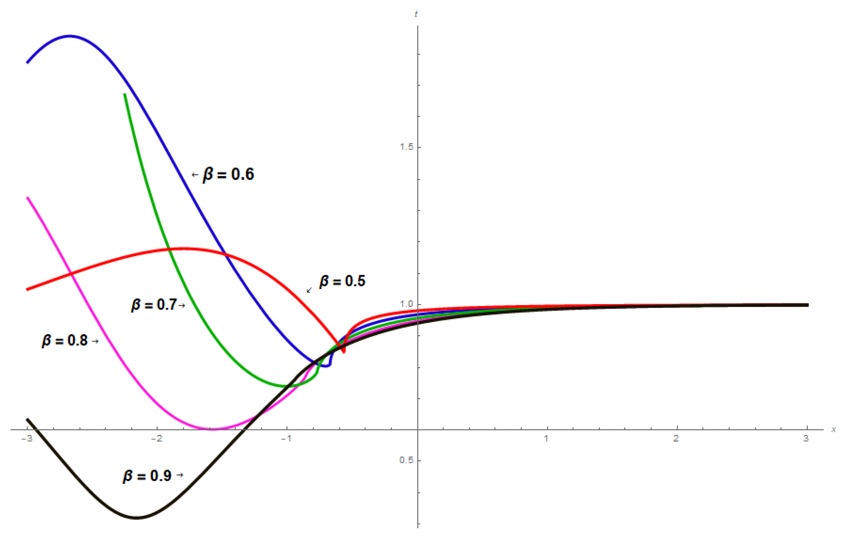
Figure 1: The analytical solution $\mid L_6(t,x)\mid$ is based on the constant values of the proposed parameters. $\mid L_6(t,x)\mid$ is graphically illustrated to demonstrate the potentiality of the EDAT with the fractional beta derivative as follows. This illustration portrays a realistic representation of $\mid L_6(t,x)\mid$ which is linked to the category of dark solitary wave solutions. Here is a visual showing a 2D-plot spanning the range $(-0.3,0.3)$ for various values of $\beta$ associated with parameters, such as $\rho =e,$$l=\sqrt{2}$, $c=1$, $\alpha =-1$, $s_1=\frac{1}{2}$, ${\mu }_1=1,$${\zeta }_1=2,$${\nu }_1=3,$ $\beta =0.5$ (red), $\beta =0.6$ (blue), $\beta =0.7$ (green), $\beta =0.8$ (magenta), $\beta =0.9$ (black).

Hence, $\mid L_6(t,x)\mid$ becomes

$$\mid L_6(t,x)\mid =\mid \left[3+4\left(-\frac{3}{4}-\frac{1}{4}tanh\left(\frac{\delta }{2}\right)\right)\right]\mid .$$

Additionally,

$$e^{\sqrt{-1}{\Theta }_1}=1,$$

$$\delta =\frac{l}{\beta }{\left(x+\frac{1}{\Gamma \left(\beta \right)}\right)}^{\beta }+\frac{c}{\beta }{\left(t+\frac{1}{\Gamma \left(\beta \right)}\right)}^{\beta }.$$

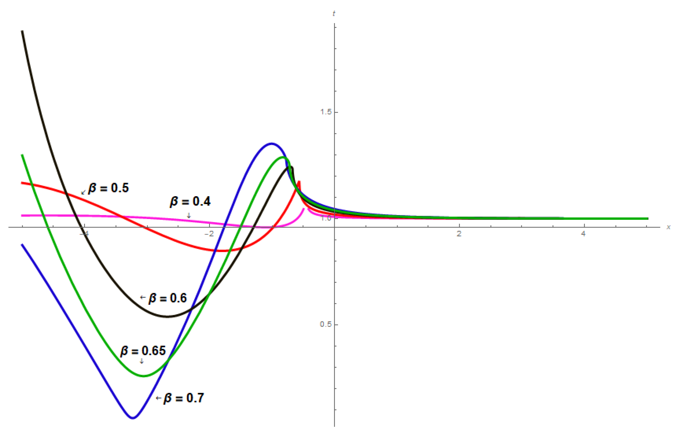
Figure 2: The analytical solution $\mid L_{10}(t,x)\mid$ is based on the constant values of the proposed parameters. $\mid L_{10}(t,x)\mid$ is graphically illustrated to demonstrate the potentiality of the EDAT with the fractional beta derivative as follows. This illustration portrays a realistic representation of $\mid L_{10}(t,x)\mid$ which is linked to the category of dark, singular solitary-wave solutions. Here is a visual showing a 2D plot spanning the range $(-0.5,0.5)$ for various values of $\beta$ associated with parameters, such as $\rho =e,$$l=\sqrt{2}$, $c=1$, $\alpha =-1$, $s_1=\frac{1}{2}$, ${\mu }_1=1,$${\zeta }_1=2,$${\nu }_1=3,$ $\beta =0.5$ (red), $\beta =0.7$ (blue), $\beta =0.65$ (green), $\beta =0.4$ (magenta), $\beta =0.6$ (black).

Hence, $\mid L_{10}(t,x)\mid$ becomes

$$\mid L_{10}(t,x)\mid =\mid \left[3+4\left(-\frac{3}{4}-\frac{1}{8}\left(tanh\left(\frac{\delta }{4}\right)+coth\left(\frac{\delta }{4}\right)\right)\right)\right]\mid .$$

Additionally,

$$e^{\sqrt{-1}{\Theta }_1}=1,$$

$$\delta =\frac{l}{\beta }{\left(x+\frac{1}{\Gamma \left(\beta \right)}\right)}^{\beta }+\frac{c}{\beta }{\left(t+\frac{1}{\Gamma \left(\beta \right)}\right)}^{\beta }.$$

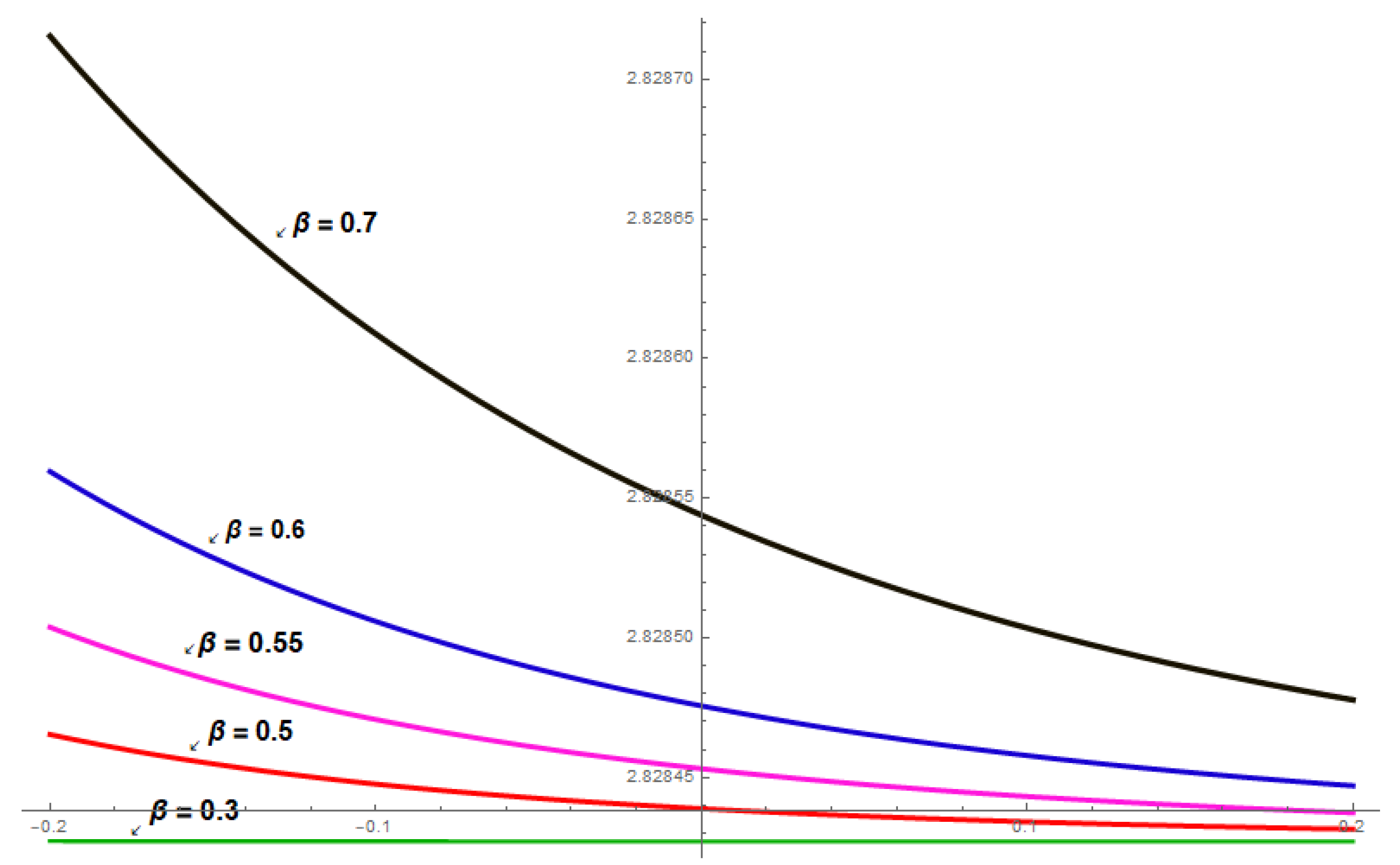
Figure 3: The analytical solution $\mid L_{18}(t,x)\mid$ is based on the constant values of the proposed parameters. $\mid L_{18}(t,x)\mid$ is graphically illustrated to demonstrate the potentiality of the EDAT with the fractional beta derivative as follows. This illustration portrays a realistic representation of $\mid L_{18}(t,x)\mid$ which is related to the category of dark–bright solitary-wave solutions. Here is a visual showing a 2D plot spanning the range $(-0.2,0.2)$ for various values of $\beta$ associated with parameters, such as $\rho =e,$$l=\sqrt{2}$, $c=1$, $\alpha =-1$, $s_1=\frac{1}{2}$, ${\mu }_1=-1,$${\zeta }_1=2,$${\nu }_1=0,$$m=-1$, $n=1$, $\beta =0.5$ (red), $\beta =0.6$ (blue), $\beta =0.3$ (green), $\beta =0.55$ (magenta), $\beta =0.7$ (black).

Hence, $\mid L_{18}(t,x)\mid$ becomes

$$\mid L_{18}(t,x)\mid =\mid \left[4\left(\sqrt{\frac{1}{2}}\left(-tanh\left(2\sqrt{2}\delta \right)-sech\left(2\sqrt{2}\delta \right)\right)\right)\right]\mid .$$

Additionally,

$$e^{\sqrt{-1}{\Theta }_1}=1,$$

$$\delta =\frac{l}{\beta }{\left(x+\frac{1}{\Gamma \left(\beta \right)}\right)}^{\beta }+\frac{c}{\beta }{\left(t+\frac{1}{\Gamma \left(\beta \right)}\right)}^{\beta }.$$

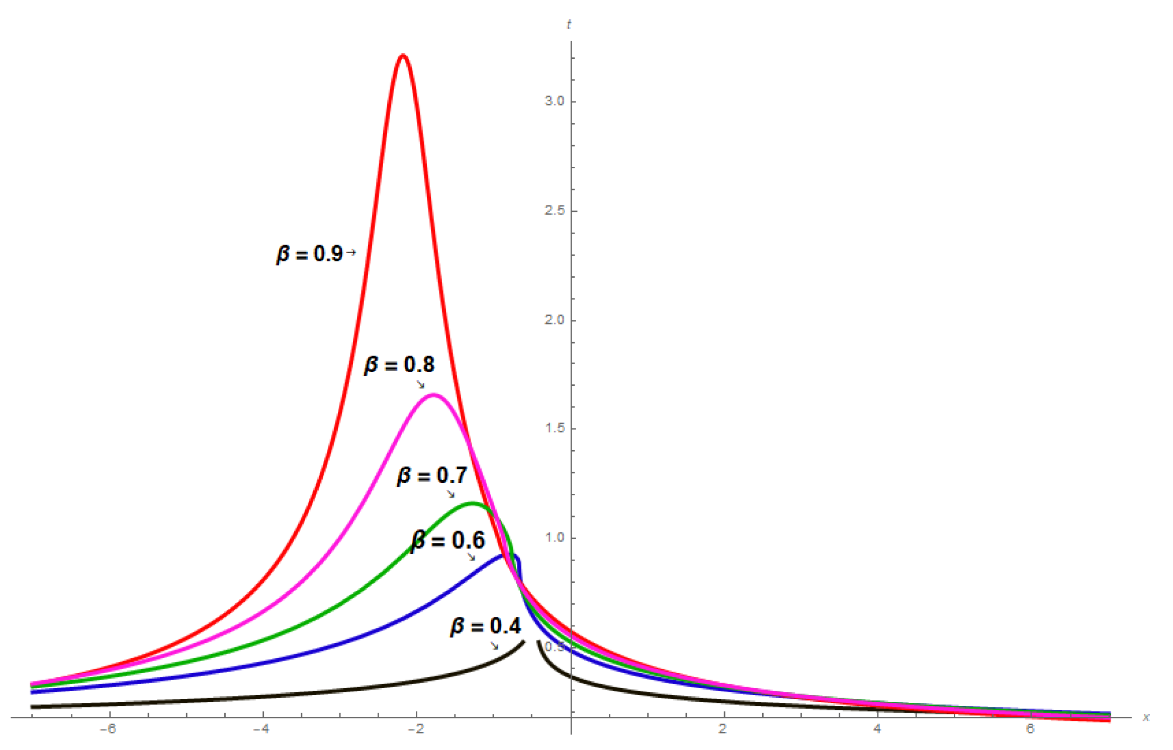
Figure 4: The analytical solution $\mid L_{31}(t,x)\mid$ is based on the constant values of the proposed parameters. $\mid L_{31}(t,x)\mid$ is graphically illustrated to demonstrate the potentiality of the EDAT with the fractional beta derivative as follows. Here is a visual showing a 2D plot spanning the range $(-0.7,0.7)$ for various values of $\beta$ associated with parameters, such as $\rho =e,$$l=\sqrt{2}$, $c=1$, $\alpha =-1$, $s_1=\frac{1}{2}$, ${\mu }_1=\frac{1}{4},$${\zeta }_1=9$, ${\nu }_1^2=9,$ $\beta =0.9$ (red), $\beta =0.6$ (blue), $\beta =0.7$ (green), $\beta =0.8$ (magenta), $\beta =0.5$ (black).

Hence, $\mid L_{31}(t,x)\mid$ becomes

$$\mid L_{31}(t,x)\mid =\mid \left[\sqrt{9}+18\left(\frac{-\frac{1}{2}(2+3\delta )}{9\delta }\right)\right]\mid .$$

Additionally,

$$e^{\sqrt{-1}{\Theta }_1}=1,$$

$$\delta =\frac{l}{\beta }{\left(x+\frac{1}{\Gamma \left(\beta \right)}\right)}^{\beta }+\frac{c}{\beta }{\left(t+\frac{1}{\Gamma \left(\beta \right)}\right)}^{\beta }.$$

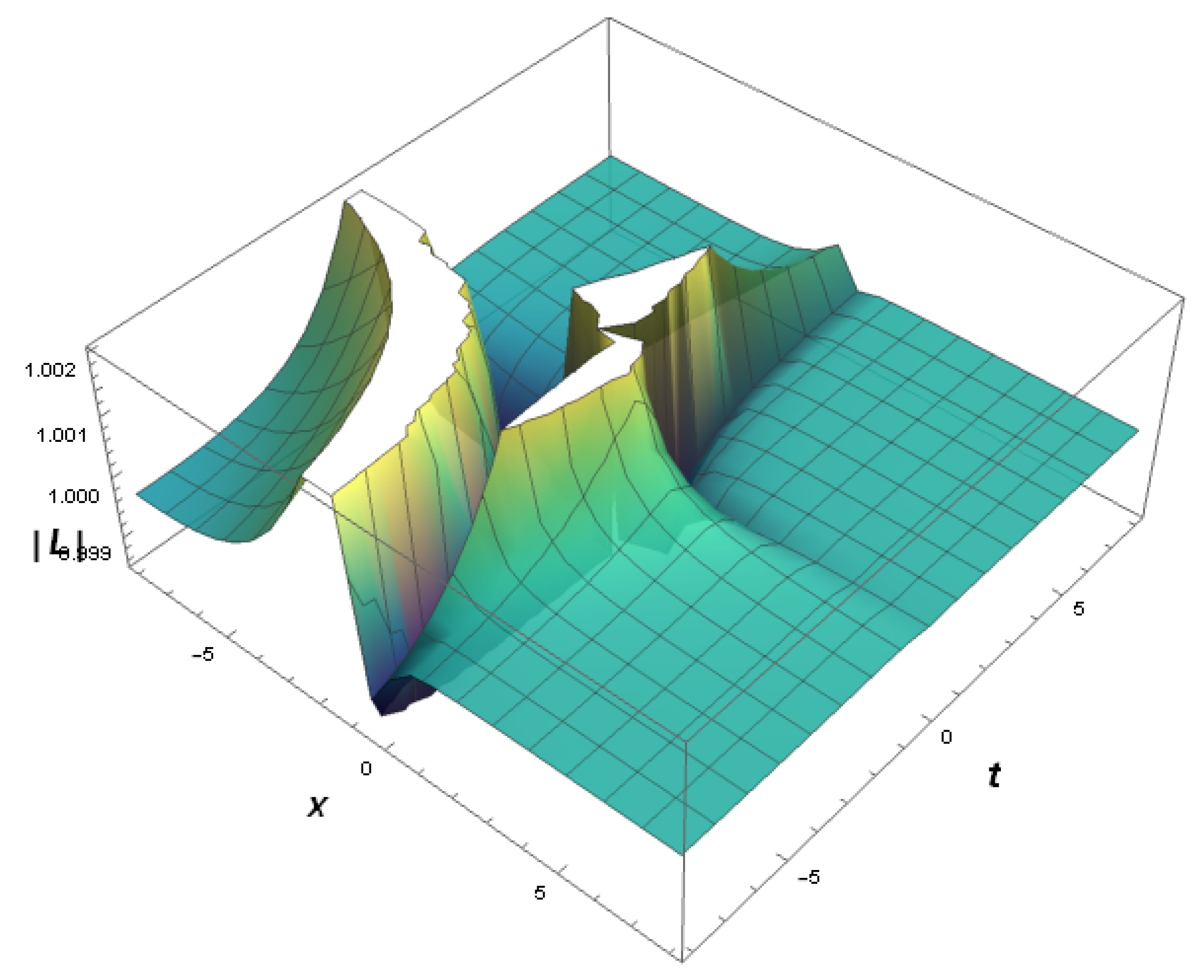
Figure 5: This illustration portrays a realistic representation of $\mid L_6(t,x)\mid$, which is linked to the category of dark solitary-wave solutions. Here is a visual showing a 3D plot spanning the range $(-0.8,0.8)$ for various values of $\beta$ associated with parameters, such as $\rho =e,$$l=\sqrt{2}$, $c=1$, $\alpha =-1$, $s_1=\frac{1}{2}$, ${\mu }_1=1,$${\zeta }_1=2,$${\nu }_1=3,$ $\beta =0.3$.

Hence, $\mid L_6(t,x)\mid$ becomes

$$\mid L_6(t,x)\mid =\mid \left[3+4\left(-\frac{3}{4}-\frac{1}{4}tanh\left(\frac{\delta }{2}\right)\right)\right]\mid .$$

As

$$\delta =\frac{\sqrt{2}}{\beta }{\left(x+\frac{1}{\Gamma \left(\beta \right)}\right)}^{\beta }+\frac{1}{\beta }{\left(t+\frac{1}{\Gamma \left(\beta \right)}\right)}^{\beta }.$$

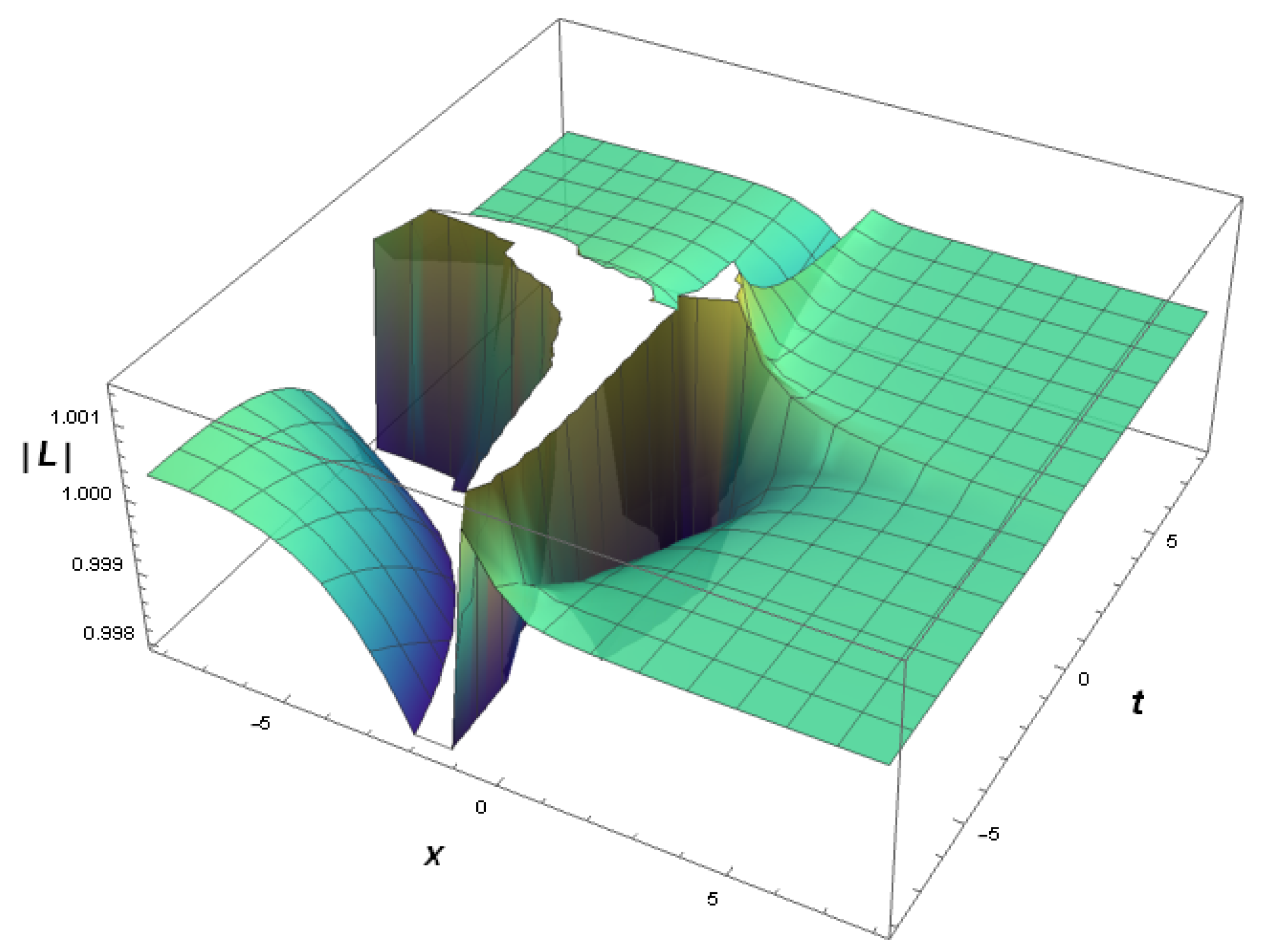
Figure 6: This illustration portrays a realistic representation of $\mid L_{10}(t,x)\mid$ which is linked to the category of dark, singular solitary-wave solutions. Here is a visual showing a 3D plot spanning the range $(-0.5,0.5)$ for various values of $\beta$ associated with parameters, such as $\rho =e,$$l=\sqrt{2}$, $c=1$, $\alpha =-1$, $s_1=\frac{1}{2}$, ${\mu }_1=1,$${\zeta }_1=2,$${\nu }_1=3,$ $\beta =0.3$.

Hence, $\mid L_{10}(t,x)\mid$ becomes

$$\mid L_{10}(t,x)\mid =\mid \left[3+4\left(-\frac{3}{4}-\frac{1}{8}\left(tanh\left(\frac{\delta }{4}\right)+coth\left(\frac{\delta }{4}\right)\right)\right)\right]\mid .$$

Additionally,

$$\delta =\frac{\sqrt{2}}{\beta }{\left(x+\frac{1}{\Gamma \left(\beta \right)}\right)}^{\beta }+\frac{1}{\beta }{\left(t+\frac{1}{\Gamma \left(\beta \right)}\right)}^{\beta }.$$

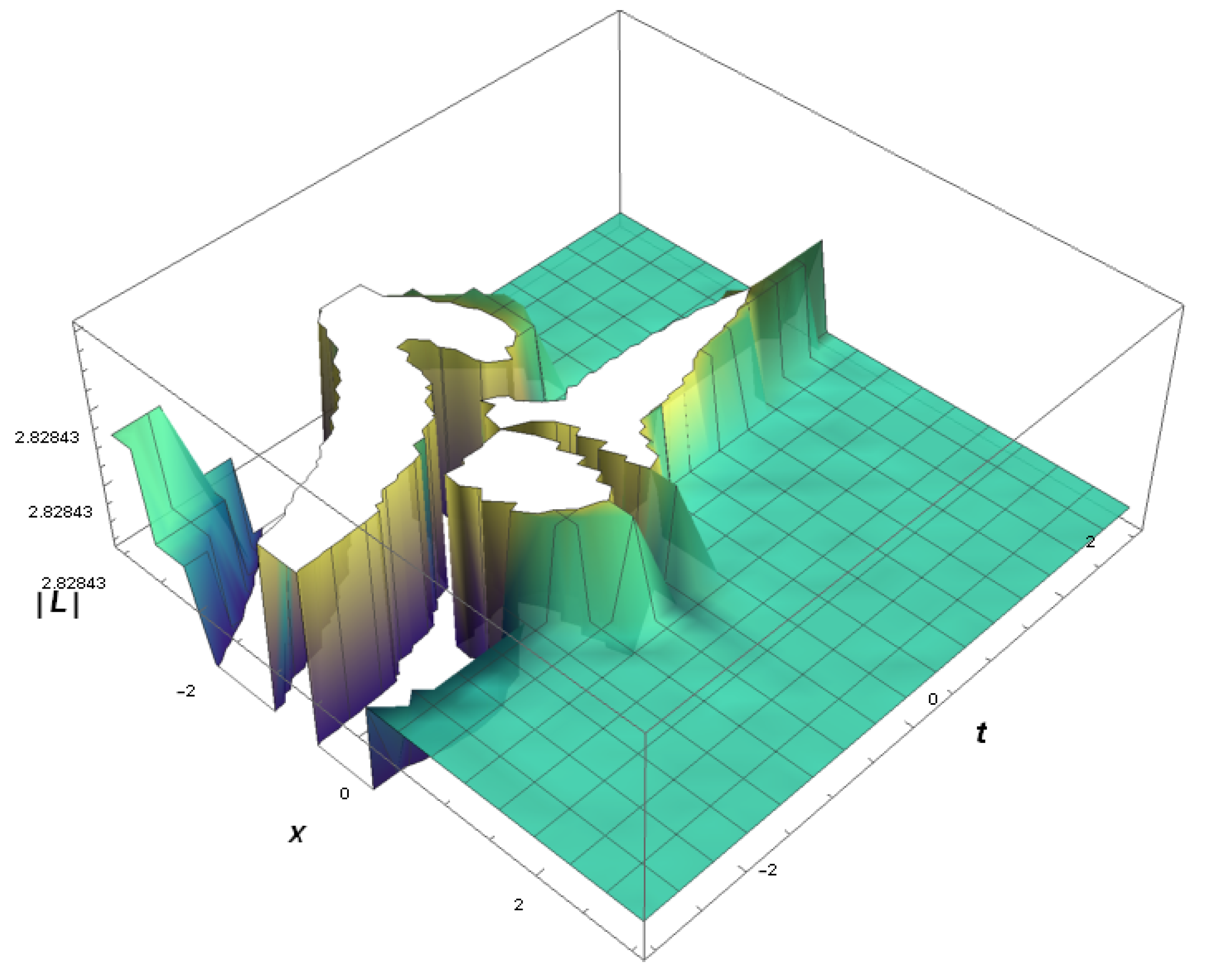
Figure 7: This illustration portrays a realistic representation of $\mid L_{18}(t,x)\mid$ which is linked to the category of dark–bright solitary-wave solutions. Here is a visual showing a 3D plot spanning the range $(-0.8,0.8)$ for various values of $\beta$ associated with parameters, such as $\rho =e,$$l=\sqrt{2}$, $c=1$, $\alpha =-1$, $s_1=\frac{1}{2}$, ${\mu }_1=-1,$${\zeta }_1=2,$${\nu }_1=0,$$m=-1$, $n=1$, $\beta =0.3$.

Hence, $\mid L_{18}(t,x)\mid$ becomes

$$\mid L_{18}(t,x)\mid =\mid \left[4\left(\sqrt{\frac{1}{2}}\left(-tanh\left(2\sqrt{2}\delta \right)-sech\left(2\sqrt{2}\delta \right)\right)\right)\right]\mid .$$

Additionally,

$$\delta =\frac{\sqrt{2}}{\beta }{\left(x+\frac{1}{\Gamma \left(\beta \right)}\right)}^{\beta }+\frac{1}{\beta }{\left(t+\frac{1}{\Gamma \left(\beta \right)}\right)}^{\beta }.$$

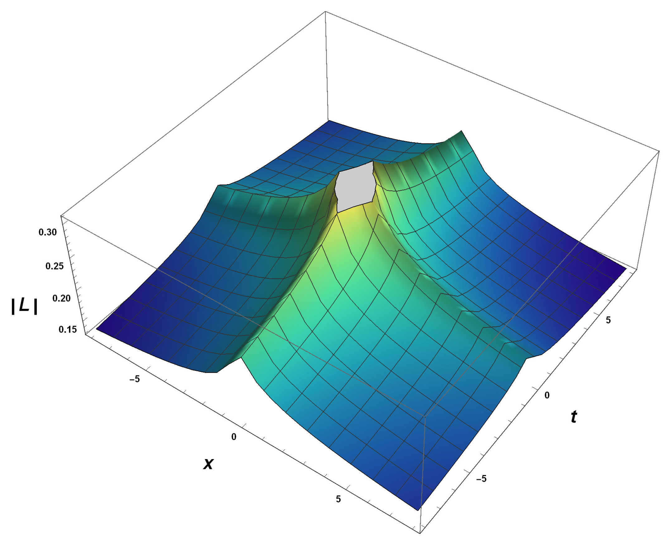
Figure 8: This illustration portrays a realistic representation of $\mid L_{31}(t,x)\mid$ which is linked to solitary-wave solutions. Here is a visual showing a 3D plot spanning the range $(-0.8,0.8)$ for various values of $\beta$ associated with parameters, such as $\rho =e,$$l=\sqrt{2}$, $c=1$, $\alpha =-1$, $s_1=\frac{1}{2}$, ${\mu }_1=\frac{1}{4},$${\zeta }_1=9$, ${\nu }_1^2=9,$ $\beta =0.3$.

Hence, $\mid L_{31}(t,x)\mid$ becomes

$$\mid L_{31}(t,x)\mid =\mid \left[\sqrt{9}+18\left(\frac{-\frac{1}{2}(2+3\delta )}{9\delta }\right)\right]\mid .$$

Additionally,

$$\delta =\frac{\sqrt{2}}{\beta }{\left(x+\frac{1}{\Gamma \left(\beta \right)}\right)}^{\beta }+\frac{1}{\beta }{\left(t+\frac{1}{\Gamma \left(\beta \right)}\right)}^{\beta }.$$

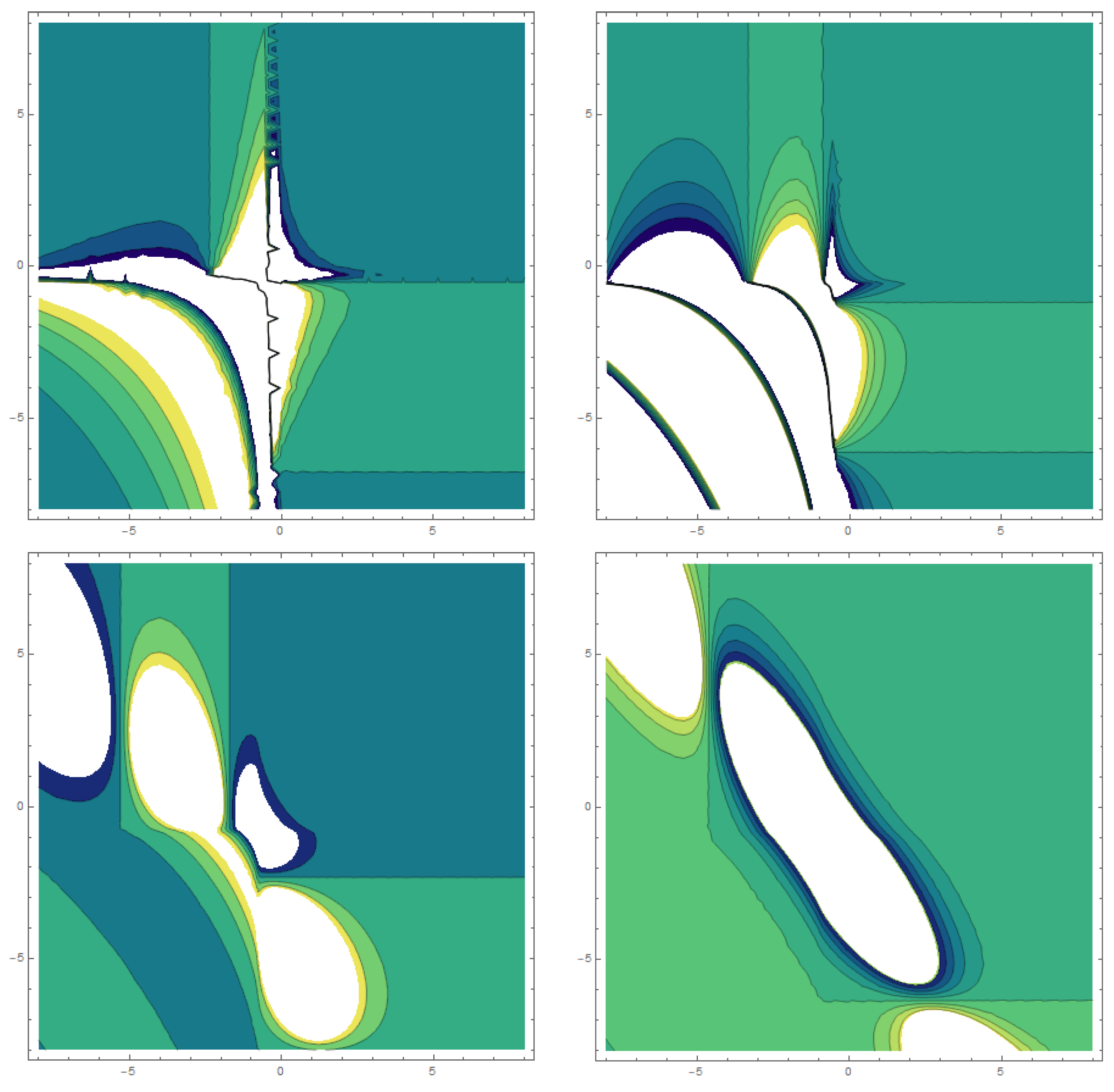
Figure 9: A contour plot is a computational technique for viewing the 3D plane on a 2D structure via representing constant “$\mid L\mid$” sheets, also known as contours. A $2D$ representation of a $3D$ surface plot is a contour plot. Contour plots are available in several general-purpose mathematical research kits. So they work on a wide range of overall visualization and math programs as well.

That illustration portrays a realistic representation of $\mid L_6(t,x)\mid$, which is linked to the category of dark solitary-wave solutions. Here is a visual showing a 2D contour spanning the range $(-0.8,0.8)$ for various values of $\beta$ associated with parameters, such as $\rho =e,$$l=\sqrt{2}$, $c=1$, $\alpha =-1$, $s_1=\frac{1}{2}$, ${\mu }_1=1,$${\zeta }_1=2,$${\nu }_1=3$, where $\beta =0.3,0.5,0.7,0.9$ in the figures below from the upper left to lower down the right side, respectively.

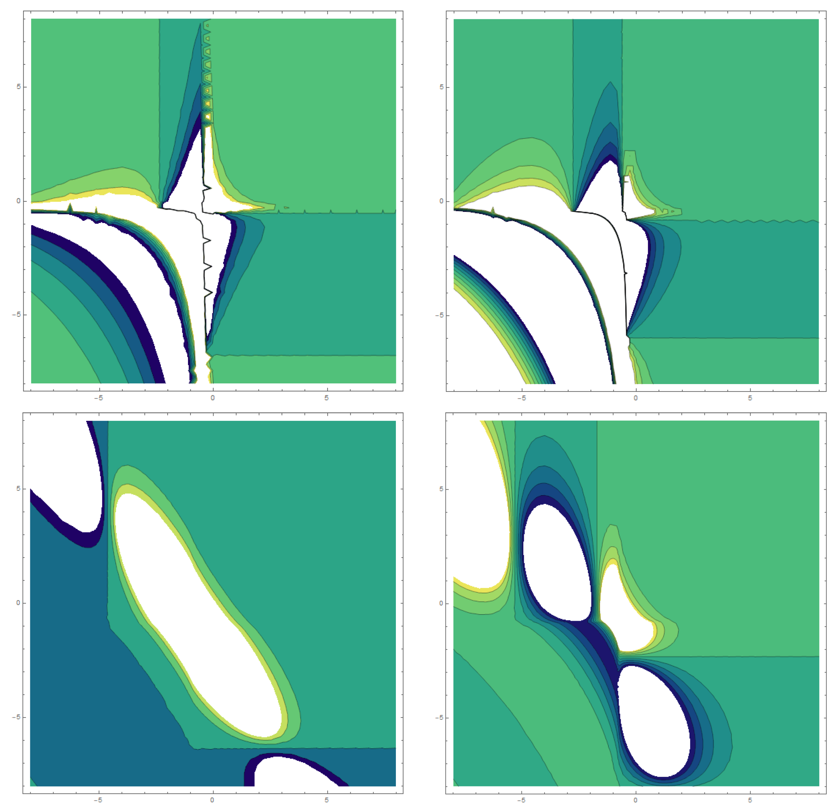
Figure 10: This illustration portrays a realistic representation of $\mid L_{10}(t,x)\mid$ which is linked to the category of dark, singular solitary-wave solutions. Here is a graphic representation of a 3D plot over the interval $(-0.5,0.5)$ for different values of $\beta$, along with the parameters, such as $\rho =e,l=\sqrt{2},c=1,\alpha =-1,s_1=\frac{1}{2},{\mu }_1=1,{\zeta }_1=2,{\nu }_1=3,$ where $\beta =0.3,0.4,0.7,0.9$ in the figures below from the upper left to lower down the right side, respectively.

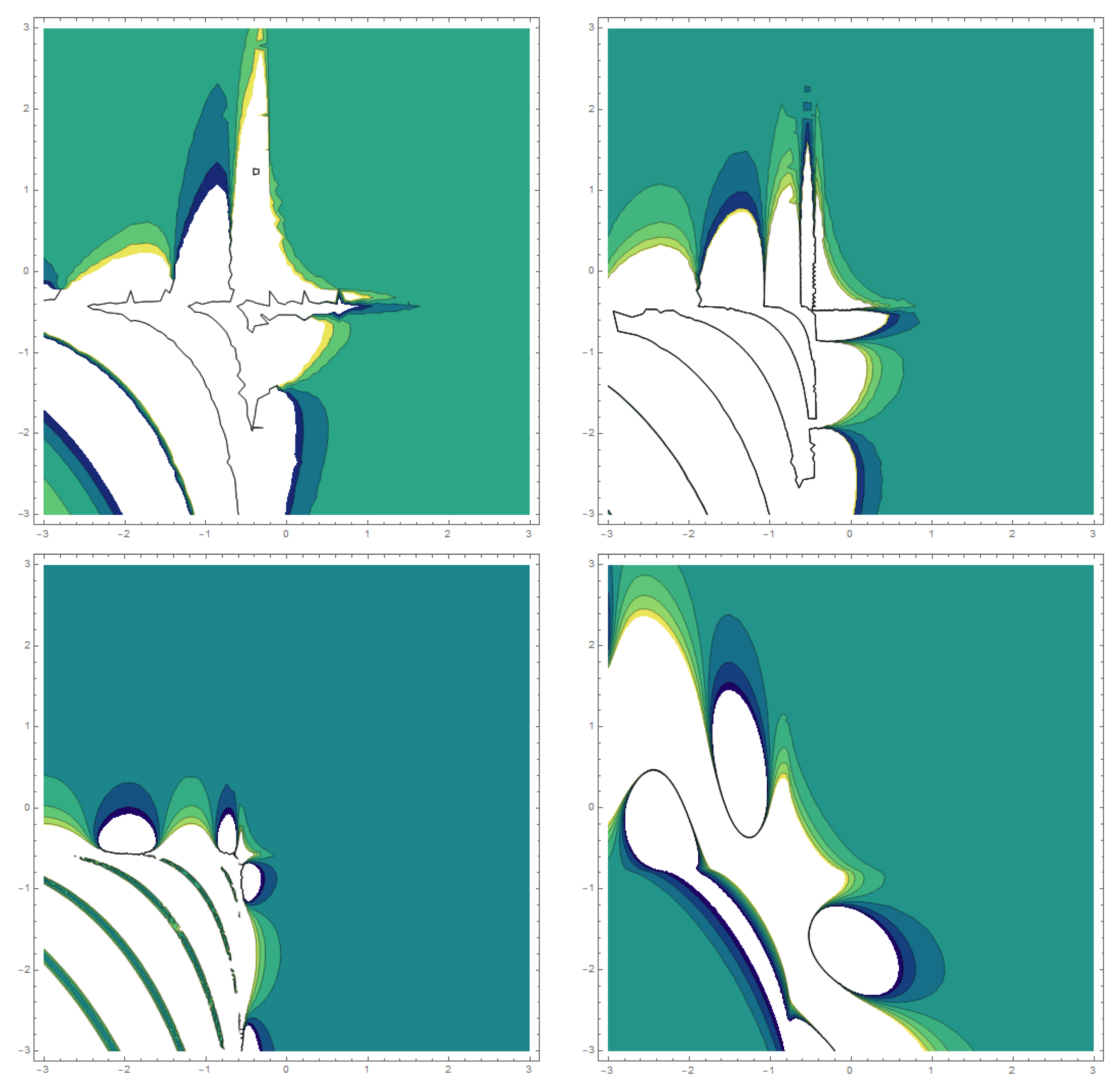
Figure 11: This illustration portrays a realistic representation of $\mid L_{18}(t,x)\mid$ which is linked to the category of dark–bright solitary-wave solutions. Here is a visual showing a 3D plot spanning the range $(-0.8,0.8)$ for various values of $\beta$ associated with parameters, such as $\rho =e,l=\sqrt{2},c=1,\alpha =-1,s_1=\frac{1}{2},{\mu }_1=-1,{\zeta }_1=2,{\nu }_1=0,m=-1,n=1,$ where $\beta =0.3,0.4,0.7,0.9$ in the figures below from the upper left to lower down the right side, respectively.

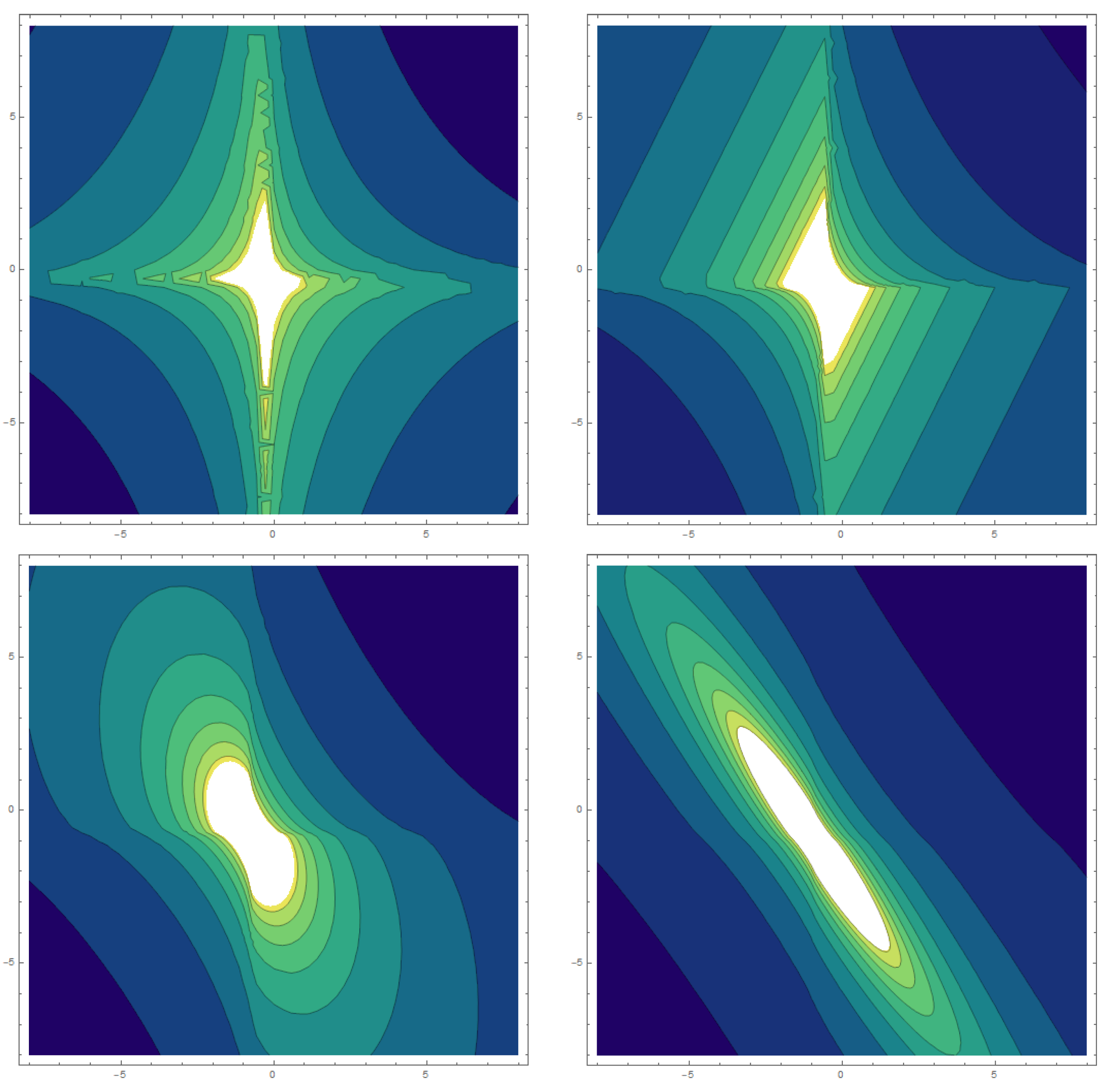
Figure 12: This illustration portrays a realistic representation of $\mid L_{31}(t,x)\mid$ which is linked to solitary-wave solutions. Here is a visual showing a 3D plot spanning the range $(-0.8,0.8)$ for various values of $\beta$ associated with parameters, such as $\rho =e,l=\sqrt{2},c=1,\alpha =-1,s_1=\frac{1}{2},{\mu }_1=\frac{1}{4},{\zeta }_1=9,{\nu }_1^2=9,$ where $\beta =0.3,0.5,0.7,0.9$ in the figures below from the upper left to lower down the right side, respectively.

6. The Sensitivity Analysis

From Equation (58), we can derive the following system:

$$H_p^{{}^{″}}=\frac{1}{\alpha l^2}(\alpha {\omega }^2+\kappa +k_p)H_p-\frac{s_p}{\alpha l^2}{H}_p^3,$$

(61)

Equation (61) can be written as

$$H_p^{{}^{″}}=h_1{H}_p+h_2{H}_p^3,$$

(62)

where, $H_p^{{}^{\prime }}=\frac{d{H}_p}{d\delta }$, $h_1=\frac{1}{\alpha l^2}(\alpha {\omega }^2+\kappa +k_p)$, $h_2=-\frac{s_p}{\alpha l^2}$.

A planer dynamical system can also represent Equation (62) by using the following short form:

$$\left\{\begin{array}{cc}{H}^{{}^{\prime }}=\hfill & u,\hfill \\ u^{{}^{\prime }}=\hfill & h_1{H}_p+h_2{H}_p^3\hfill \end{array}\right.$$

(63)

We will right away look at the delicate phenomena of the disturbed system displayed below. The autonomous conservative dynamical system $\left(ACDS\right)$ then decomposes the schemes of Equation (62), as shown below:

$$\left\{\begin{array}{cc}{H}^{{}^{\prime }}=\hfill & u,\hfill \\ u^{{}^{\prime }}=\hfill & h_1{H}_p+h_2{H}_p^3+n_{0}cos{f}^{*}\delta ,\hfill \end{array}\right.$$

(64)

where $n_0$ is the intensity of the disturbed component [24], and $f^{*}$ seems to be the frequency. The system of Ref. (64) exhibits a superficial periodic force, but the system of Ref. (63) does not. To examine the sensitive behavior of Equation (58) in the appearance of a perturbation component, including the parameters $h_1$ and $h_2$, we would look into seeing if the frequency term has any effect on the model that is being discussed in the present section of the study. To achieve this, we will ascertain the model under the examination’s physical characteristics and clarify how the force and frequency of the disturbance affect the system.

To do so, we will apply the following special beginning conditions to the component to test the component’s sensitivity for such a solution of the perturbed dynamical structural scheme from (64):

Even if all of the components in the figures, from (a) to (d), have the same remaining parameters, the following are the parametric constraints:

$$\rho =e,l=\sqrt{2},\kappa =0.8,k_p=0.6,\omega =\alpha =1,s_p=\frac{1}{2},$$

$$h_1=1.2,h_2=-0.25,n_0=3.2,f^{*}=0.85.$$

To ascertain how sensitive our system is, we conduct a sensitivity study shown in

Table 1. Sensitivity Study.

Sensitivity Assessment
Figure	Solid Blue Line	Red Doted Curve
(a)	(0.00, 0.00)	(0.10, 0.10)
(b)	(0.10, 0.10)	(0.15, 0.15)
(c)	(0.08, 0.08)	(0.16, 0.16)
(d)	(0.15, 0.15)	(0.30, 0.30)

. The system will have low sensitivity if it only changes somewhat as a result of slight changes to the original circumstances. The system will, however, be particularly sensitive if there is a big adjustment as a result of a little change in the beginning circumstances. The waves’ changing amplitude patterns are depicted in the figures below. Because these curves do not overlap, the system is sensitive to these changes.

In Figure 13a, the plot shows the sensitivity illustrating the dynamical system (64), assuming the similar parameters as stated earlier for the initial constraints as $(H_p,\delta )=(0,0)$ in the red dotted curve and $(H_p,\delta )=(0.10,0.10)$ throughout solid blue line. The system has very low sensitivity from the beginning (i.e., 0 to 20) and the system has high sensitivity till the end (i.e., 20 to 50). In Figure 13b, the model is sensitive between (30 to 40). In Figure 13c, the model is sensitive between (30 to 50), and in Figure 13d, the model is sensitive between (10 to 50). Furthermore, the details of these figures are described in the above table.

7. Analysis of Results and Discussions

In order to understand physical problems in nonlinear optics, such as the dimensionless types of optical fields in the corresponding cores of optical fibers, L and M are computed in aspects of distinctive mathematical functions and beta derivative evolution to separate a compact soliton from its wide and growing pedestal. Due to the inclusion of an arbitrary functional structure and coupling terms, Equations (47) and (61) are not necessarily entirely integrable. As a result, the solitary wave solutions are built using a very productive mathematical methodology, i.e., the extended direct algebraic approach. From the analytical solutions of the defined equations, many kinds of solitary waves solutions are being extracted. It is also discovered that when $\beta$ is between 0 and 1, the wave structures are greatly affected by the beta fractional parameter. We plotted 3D-, and 2D-contour graphs over distinct and discrete intervals for effective illustration based on their physical ranges; corresponding numerical values for parameters were used as part of our experiment to examine different dynamic behaviors, patterns, and textures of solitary-wave solutions.

In the below three plots, one can easily observe that by changing the values of $\alpha$ in the dark solitary-wave solution that is occurring in the upper left corner of Figure 14, the curve is not just translating along the ordinate. It is also changing its amplitude by increasing the value of dispersion coefficient $\alpha$, and the amplitude of the wave is decreasing. So the amplitude is inversely proportional to the value of the dispersion coefficient. Furthermore, by either varying the values of $\alpha$ within semi-dark solitary-wave solutions shown in the upper right edge of Figure 14, the curve not only moves across the ordinate, but also changes its amplitude, as increasing the value of the dispersion coefficient $\alpha$ increases the amplitude of the wave. As a result, the amplitude is directly proportional to the value of the dispersion coefficient. Additionally, by changing the values of $\alpha$ in the last plot of Figure 14, the amplitude of the wave is increasing by increasing the value of dispersion coefficient $\alpha$. Hence, the amplitude is proportional to the value of the dispersion coefficient.

We saw various textures of solitary waves in the 2D graphical representation of dark solitary-wave solutions, which is a complex valued function reflecting the optical concerns in two cores, i.e., $\mid L_6\mid$ through different values of $\beta$, as we can see in the interval $(-0.3,0.3)$, where the amplitude structures of the dark solitary waves minimizes as the value of $\beta$ increases. The amplitude structure of the waves minimizes as the structures of the dark solitary waves for numerous different values of $\beta$ progress toward 03 in the specified interval, and all of these waves collide at a single wave of constant amplitude.

We saw various textures of solitary waves in the 2D graphical representation of dark-singular solitary-wave solutions, which is a complex valued function reflecting the optical concerns in two cores, i.e., $\mid L_{10}\mid$ through different values of $\beta$, as we can see in the interval $(-0.5,0.5)$, where the amplitude structures of the dark singular solitary waves increases as the value of $\beta$ increases. The amplitude structure of the waves minimizes as the structures of the dark solitary waves for numerous different values of $\beta$ progress toward 05 in the specified interval, and all of these waves collide at a single wave of constant amplitude.

We saw various textures of solitary wave in 2D graphical representation of dark bright solitary-wave solutions, which is a complex valued function reflecting the optical concerns in two cores, i.e., $\mid L_{18}\mid$ through different values of $\beta$, as we can see in the interval $(-0.2,0.2)$, where the amplitude structures of the dark–bright solitary waves increases as the value of $\beta$ increases. The amplitude structure of the waves minimizes as the structures of the dark solitary waves for numerous different values of $\beta$ progress toward $0.2$ in the specified interval. The amplitude structures of all the dark–bright solitary waves minimizes.

We saw various textures of solitary waves in the 2D graphical representation of solitary-wave solutions, which is a complex-valued function reflecting the optical concerns in two cores, i.e., $\mid L_{31}\mid$ through different values of $\beta$, as we can see in the interval $(-0.7,0.7)$, where the amplitude structures of the solitary waves increases as the value of $\beta$ increases. The amplitude structure of the waves minimizes as the structures of the dark solitary waves for numerous different values of $\beta$ progress toward 07 in the specified interval, and all of these waves collide at a single wave of zero amplitude.

8. Comparative Investigation via Different Fractional Derivatives

Because of the different descriptions of FDs (conformable, modified Riemann–Liouville, beta derivative, etc.), fractional model solutions offer unique physical observations and applications when the fractional value of these FDs is taken into account. It is exceedingly challenging for scientists to determine which of the FDs is the most accurate and reliable. In this part, meanwhile, a comparison of the solutions found in this study with those derived by the use of the modified Riemann–Liouville and beta derivative is provided. Teodoro et al. [25] conducted a thorough examination of the definitions and characteristics of modified Riemann–Liouville and beta derivatives. It should be noted here that the transformations, $L(x,t)=H\left(\delta \right)$, $\xi =l\frac{x^{\beta }}{\Gamma (1+\beta )}+c\frac{t^{\beta }}{\Gamma (1+\beta )},$ for the modified Riemann-Liouville derivative, $L(x,t)=H\left(\delta \right)$, $\delta =l\frac{x^{\alpha }}{\alpha }+c\frac{t^{\alpha }}{\alpha },$ for conformal derivative, and $L(x,t)=H\left(\delta \right)$, $\delta =\frac{l}{\beta }{\left(x+\frac{1}{\Gamma \left(\beta \right)}\right)}^{\beta }+\frac{c}{\beta }{\left(t+\frac{1}{\Gamma \left(\beta \right)}\right)}^{\beta },$ for the beta derivative are utilized for Equations (42) and (43), and the ODE described by Equation (58) is derived. Two-wave solutions are provided in each case to compare the performance of the findings produced in this analysis with those achieved using the modified Riemann–Liouville and beta derivatives. The solutions $L_6$, and $L_{13}$ produced with the sense of the beta derivative are created with the concept of the modified Riemann–Liouville and conformal derivatives, respectively, and thus are stated as follows:

We provide the findings by the corresponding FD in Figure 15 and Figure 16 to compare the accuracy and reliability of our generated solutions via the beta FD with those acquired by the modified Riemann–Liouville FD and conformal FD. The trend of all solution profiles for the stated derivatives can be seen in all these figures below, but the solutions produced in this investigation can be determined to be in significant association with those derivatives.

9. Conclusions

Twin-core $NLDCs$ via $OMMs$ with spatial–temporal $BDE$, including Kerr law nonlinearity, are addressed in this study. The EDAT was used to generate analytical solutions for these equations. The results were expressed using a variety of mathematical functions with the beta derivative and other associated parameters. The respondents to the proposed equations were discovered in truly innovative ways as a result of $BDE$, indicating that no comparisons with the preceding studies are needed. This research is not only concerned with $BDE$, but also with the efficacy of such a method for obtaining solitary-wave solutions to model equations. The findings of this research will aid in understanding not only wave transmission activities in nonlinear sciences, specifically nonlinear optics, but also future laboratory studies, where the proposed model equation is generally applicable. It can also be remembered that the EDAT can be used with $BDE$ to find the analytical solutions to every other nonlinear evolution equation, but this is outside the reach of this research.

Using the trial function approach [13], this study provides soliton solutions to nonlinear directional couplers in optical metamaterials. Three different types of couplers are investigated. Solutions for bright, dark, and solitary solitons are found. In [15], the analytical solutions for modeling $NLDCs$ with $MMs$ using spatial–temporal fractional $BDE$ are presented in this study. To ensure such solutions, the auxiliary ordinary differential equation technique and the generalized Riccati method with beta derivative characteristics are used. Through nonlinear optics [26], a fractional comparison assessment of nonlinear directional couplers is performed. The found solutions are Atangana–Baleanu fractional solitons containing a modified Riemann–Liouville fractional operator. Furthermore, in comparison to the previously stated publications, our contribution is more broad in that we investigate soliton solutions and sensitivity analyses for $NLDCs$ through $OMMs$ with spatial–temporal $BDE$, incorporating Kerr law nonlinearity, where it has not before been done in the literature. Additionally, the analytical approach is more broadly extended and produces many forms of soliton solutions.

The EDAT is very skilled and practically developed for the following: obtaining new analytical solutions of nonlinear differential equations; determining the exact solution in a well-understood manner; employing a computation system easier and faster; being an effective method to tackle the various aspects of analytical solitary solutions; and having outcomes that are more comprehensively generalized. These are the most important characteristics of the EDAT because the approach is recent and can handle a wider range of functions, including several types of soliton solutions. As an excellent example, it appears that the 6th, 16th and 26th are dark soliton solutions (a hyperbolic tangent, or dark soliton), which are solitons from the standpoint that they propagate without abruptly changing shape, but which are not created by a regular pulse but rather by a lack of energy in a continuous time beam. With the exception of a brief time where it briefly goes to zero and then quickly increases again, the intensity is continuous, producing a black pulse. Such solitons can be created by introducing brief dark pulses within much longer regular pulses.

The 8th, 18th and 28th have semi-dark soliton solutions, and neither the hyperbolic tangent nor the hyperbolic cotangent were producedby a regular pulse but rather by an energy deficiency in a continuous-time beam. As in this pulse, when there is both crust and trough (rising and reducing behavior in the same pulse), the intensity stays constant, with the exception of a brief time during which it goes to zero and then rises again. This results in a pulse that is either semi-dark or semi-bright. Similar to this, the 10th, 20th and 30th indicate dark singular solutions (hyperbolic tangent and cotangent), whereas the 9th, 19th and 29th appear to be Type 1 and Type 2 solitary solutions (hyperbolic cotangent and hyperbolic cosecant), and 7th, 17th and 27th are Type 2 singular solutions (hyperbolic cotangent).

Additionally, the implementations of these theoretical solutions are in meta-material, including optical filters, sensor recognition, telecommunications assessment, high-frequency battlefield connectivity, and optical fibers, but also lenses for high-gain transmitters.

References

- Bahrami, A.; Rostami, A.; Nazari, F. MZ-MMI-based all optical witch using nonlinear coupled waveguides. Optik 2011, 122, 1787. [Google Scholar] [CrossRef]
- Dai, C.Q.; Wang, Y.Y. Controllable combined Peregrine soliton and Kuznetsov-Ma soliton in PT-symmetric nonlinear couplers with gain and loss. Nonlinear Dyn. 2015, 80, 715. [Google Scholar] [CrossRef]
- Savescu, M.; Bhrawy, A.H.; Alshaery, A.A.; Hilal, E.M.; Khan, K.R.; Mahmood, M.F.; Biswas, A. Optical solitons in nonlinear directional couplers with spatio-temporal dispersion. J. Mod. Opt. 2014, 442, 442. [Google Scholar] [CrossRef]
- Kumar, D.; Singh, J.; Purohit, S.D. A hybrid analytical algorithm for nonlinear fractional wave-like equations. Math. Model. Nat. Phenom. 2019, 14, 304. [Google Scholar] [CrossRef] [Green Version]
- Bhatter, S.; Mathur, A.; Kumar, D.; Singh, J. A new analysis of fractional Drinfeld-Sokolov-Wilson model with exponential memory. Phys. A Stat. Mech. Appl. 2020, 537, 122578. [Google Scholar] [CrossRef]
- Li, B.Q.; Ma, Y.L.; Yang, T.M. The oscillating collisions between the three solitons for a dual-mode fiber coupler system. Superlatt. Microstruct. 2017, 126, 110. [Google Scholar] [CrossRef]
- Mirzazadeh, M.; Eslami, M.; Zhou, Q.; Mahmood, M.F.; Zerrad, E.; Biswas, A.; Belic, M. Optical solitons in nonlinear directional couplers with G′/G-expansion scheme. J. Nonlinear Opt. Phys. Mater. 2015, 24, 1550017. [Google Scholar] [CrossRef]
- Banaja, M.; Alkhateeb, S.; Alshaery, A.; Hilal, E.M.A. Singular Optical Solitons in Nonlinear Directional Couplers. J. Comput. Theor. Nanosci. 2016, 13, 4660. [Google Scholar] [CrossRef]
- Xiang, Y.; Dai, X.; Wen, S.; Guo, J.; Fan, D. Controllable Raman soliton self-frequency shift in nonlinear metamaterials. Phys. Rev. A 2011, 84, 033815. [Google Scholar] [CrossRef] [Green Version]
- Biswas, A.; Ekici, M.; Sonmezoglud, A.; Zhoue, Q.; Moshokoac, S.P.; Belic, M. Chirped solitons in optical metamaterials with parabolic law nonlinearity by extended trial function method. Optik 2018, 92, 160. [Google Scholar] [CrossRef]
- Biswas, A.; Khan, K.R.; Mahmood, M.F.; Belic, M. Bright and dark solitons in optical metamaterials. Optik 2014, 125, 3299. [Google Scholar] [CrossRef]
- Triki, H.; Zhoub, Q.; Moshokoa, S.P.; Ullah, M.Z.; Biswas, A.; Belic, M. Novel singular solitons in optical metamaterials for self-steepening effect. Optik 2014, 154, 545. [Google Scholar] [CrossRef]
- Arnous, A.H.; Ekici, M.; Moshokoa, S.P.; Ullah, M.Z.; Biswas, A.; Belic, M. Solitons in Nonlinear Directional Couplers with Optical Metamaterials by Trial Function Scheme. Acta Phys. Pol. A 2017, 132, 1399–1410. [Google Scholar] [CrossRef]
- Vega-Guzman, J.; Mahmood, M.F.; Zhou, Q.; Triki, H.; Arnous, A.H.; Biswas, A.; Moshokoa, S.P.; Belic, M. Solitons in nonlinear directional couplers with optical Metamaterials. Nonlin. Dyn. 2017, 87, 427. [Google Scholar] [CrossRef]
- Uddin, M.F.; Hafez, M.G.; Hammouch, Z.; Rezazadeh, H.; Baleanu, D. Traveling wave with beta derivative spatialtemporal evolution for describing the nonlinear directional couplers with metamaterials via two distinct methods. Alex. Eng. J. 2021, 60, 1055–1065. [Google Scholar] [CrossRef]
- Özkan, Y.S.; Yasar, E.; Seadawy, A.R. A third-order nonlinear Schrödinger equation: The exact solutions, group-invariant solutions and conservation laws. J. Taiwan Univ. Sci. 2020, 14, 585–597. [Google Scholar] [CrossRef]
- Singh, J.; Kumar, D.; Al-Qurashi, M.; Baleanu, D. A new fractional model for giving up smoking dynamics. Adv. Differ. Equ. 2017, 2017, 88. [Google Scholar] [CrossRef] [Green Version]
- Riaz, M.B.; Atangana, A.; Iftikhar, N. Heat and mass transfer in Maxwell fluid in view of local and non-local differential operators. J. Therm. Anal. Calorim. 2020, 133, 1–17. [Google Scholar] [CrossRef]
- Riaz, M.B.; Saeed, S.T.; Baleanu, D. Role of Magnetic field on the Dynamical Analysis of Second Grade. Fluid: An Optimal Solution subject to Non-integer Differentiable Operators. J. Appl. Comput. Mech. 2021, 7, 54–68. [Google Scholar]
- Atangana, A.; Baleanu, D.; Alsaedi, A. Analysis of timefractional Hunter-Saxton equation: A model of neumatic liquid crystal. Open Phys. 2016, 14, 145. [Google Scholar] [CrossRef]
- Rezazadeh, H. New solitons solutions of the complex Ginzburg-Landau equation with Kerr law nonlinearity. Optik 2018, 167, 218–227. [Google Scholar] [CrossRef]
- Munawar, M.; Jhangeer, A.; Pervaiz, A.; Ibraheem, F. New general extended direct algebraic approach for optical solitons of Biswas-Arshed equation through birefringent fibers. Optik 2021, 228, 165790. [Google Scholar] [CrossRef]
- Jhangeer, A.; Munawar, M.; Atangana, A.; Riaz, M.B. Analysis of electron acoustic waves interaction in the presence of homogeneous unmagnetized collision-free plasma. Phys. Scr. 2021, 96, 075603. [Google Scholar] [CrossRef]
- Jhangeer, A.; Hussain, A.; Tahir, S.; Sharif, S. Solitonic, super nonlinear, periodic, quasiperiodic, chaotic waves and conservation laws of modified Zakharov-Kuznetsov equation in the transmission line. Commun. Nonlinear Sci. Numer. Simul. 2020, 86, 105254. [Google Scholar] [CrossRef]
- Teodoro, G.S.; Machado, J.T.; De Oliveira, E.C. A review of definitions of fractional derivatives and other operators. J. Comput. Phys. 2019, 388, 195–208. [Google Scholar] [CrossRef]
- Asjad, M.I.; Faridi, W.A.; Jhangeer, A.; Abu-Zinadah, H.; Ahmad, H. The fractional comparative study of the non-linear directional couplers in non-linear optics. Results Phys. 2021, 27, 104459. [Google Scholar] [CrossRef]
Figure 1.
The 2D graphs of dark solitary waves solution, i.e., across different values of .
Figure 2.
The 2D graphs of dark, singular solitary-wave solution, i.e., across different values of .
Figure 3.
The 2D graphs of dark–bright solitary-wave solution, i.e., across different values of .
Figure 4.
The 2D graphs of solitary-wave solution, i.e., across different values of .
Figure 5.
The 3D graph of dark solitary-wave solutions, i.e., across .
Figure 6.
The 3D graph of dark singular solitary-wave solutions, i.e., across .
Figure 7.
The 3D graph of dark–bright solitary-wave solutions, i.e., across .
Figure 8.
The 3D graphical representation of solitary-wave solutions, i.e., across .
Figure 9.
across different values of .
Figure 10.
The 2D contour graphs of across different values of .
Figure 11.
The 2D contour graphs of dark–bright solitary-wave solution, i.e., across different values of .
Figure 12.
Figure 13.
Sensitivity plots for the dynamical system with different initial conditions.
Figure 14.
The 2D plots of solitary-wave solution across different values of dispersion coefficient .
Figure 15.
Comparative investigation of the dark soliton solution via the modified Riemann–Liouville, conformable and beta derivatives for the fix value of fractional order defined by these fractional derivatives.
Figure 16.
Comparative investigation of the soliton solution via the modified Riemann–Liouville, conformable and beta derivatives for the fix value of fractional order defined by these fractional derivatives.