Numerical Investigation of a Class of Nonlinear Time-Dependent Delay PDEs Based on Gaussian Process Regression

Abstract

Probabilistic machine learning and data-driven methods gradually show their high efficiency in solving the forward and inverse problems of partial differential equations (PDEs). This paper will focus on investigating the forward problem of solving time-dependent nonlinear delay PDEs with multi-delays based on multi-prior numerical Gaussian processes (MP-NGPs), which are constructed by us to solve complex PDEs that may involve fractional operators, multi-delays and different types of boundary conditions. We also quantify the uncertainty of the prediction solution by the posterior distribution of the predicted solution. The core of MP-NGPs is to discretize time firstly, then a Gaussian process regression based on multi-priors is considered at each time step to obtain the solution of the next time step, and this procedure is repeated until the last time step. Different types of boundary conditions are studied in this paper, which include Dirichlet, Neumann and mixed boundary conditions. Several numerical tests are provided to show that the methods considered in this paper work well in solving nonlinear time-dependent PDEs with delay, where delay partial differential equations, delay partial integro-differential equations and delay fractional partial differential equations are considered. Furthermore, in order to improve the accuracy of the algorithm, we construct Runge–Kutta methods under the frame of multi-prior numerical Gaussian processes. The results of the numerical experiments prove that the prediction accuracy of the algorithm is obviously improved when the Runge–Kutta methods are employed.

1. Introduction

In the last decade, more and more attention has been paid on the theoretical studies and practical applications concerned with probabilistic machine learning and data-driven methods [1,2], and some studies have been gradually extended to the fields of differential equations. How to predict the solution of (nonlinear) dynamic systems represented by (delay) partial differential equations (PDEs) has been valued [3,4,5,6,7,8]. However, (deep) neural networks are favored and used more often by researchers [9,10,11,12,13,14,15,16], and the research targets may involve the forward and inverse problem [17].

Machine learning for Gaussian processes (GPs) [18] is not new, and has been wildly employed in many fields, such as geology [19], meteorology [20] and some financial applications [21]. Similar to other machine learning methodologies, Gaussian processes can be utilized in regression problems or classification problems. Moreover, Gaussian processes belong to a set of methods named kernel machines [22]. However, compared with other kernel machine methods, such as support vector machines (SVMs) [23] and relevance vector machines (RVMs) [24], the strict probability deduction of Gaussian processes greatly limits the popularization of this method in industrial circles. Another drawback of Gaussian processes is that the computational cost may be expensive, due to the Cholesky decomposition of the kernel functions. As a kernel machine with very strong learning ability, Gaussian processes (GPs) have been widely used in the forward and inverse problem of ordinary differential equations (ODEs) and PDEs in recent years.

Markus et al. (2021) [25] constructed multi-output Gaussian process priors with realizations in the solution set of the linear PDEs; the construction was fully algorithmic via Gröbner bases. However, the construction for building GP priors by the parametrization of such systems was done via a pullback. Paterne et al. (2022) [26] efficiently inferred inhomogeneous terms modeled as GPs by using a truncated basis expansion of the GP kernel from the perspective of exact conjugate Bayesian inference. Mamikon et al. (2022) [27] proposed a framework which combined co-Kriging with the linear transformation of GPs together with the use of kernels given by spectral expansions in eigenfunctions of the boundary value problem, to infer the solution of a well-posed boundary value problem (BVP). To estimate parameters of nonlinear dynamic systems, represented by ODEs from sparse and noisy data, Yang et al. (2022) [28] bypassed the need for numerical integration, and proposed a fast and accurate method, named manifold-constrained Gaussian process inference (MAGI), explicitly conditioned on the manifold constraint that derivatives of Gaussian processes must satisfy the considered ODEs, based on a GP model over time series data. Raissi et al. (2018) [29] proposed a method for the forward problem of time-dependent PDEs based on GPR, which was named numerical Gaussian processes (NGPs). The method can solve equations with high accuracy, and the frame of the algorithm is flexible for solving different problems. Generally speaking, the study of Gaussian processes is an important branch of probabilistic numerics [30,31,32,33,34,35] in numerical analysis.

On the basis of NGPs, we propose a new method, multi-prior numerical Gaussian processes (MP-NGPs), which is designed to solve complex PDEs. In our known information, most methods based on Gaussian processes do not consider the delay term and high-dimensional problems, and only a few researchers consider fractional derivatives and integro differential derivatives, which obviously cannot meet the requirements of practical application. However, these problems are all considered in MP-NGPs. We also give strict mathematical deduction of MP-NGPs. Several PDEs are solved in the following sections to prove the validity of MP-NGPs.

It is well known that Gaussian processes [18] possess a strict mathematical basis and coincide with the Bayesian method in nature. Unlike traditional methods, including the finite element method [36], spectral method [37], and finite difference method [38], MP-NGPs [29] solve PDEs by means of statistical methods, which is the same as NGPs. In MP-NGPs, the Bayesian method [39] is used to construct an efficient data learning machine, and then infer the solution of the equations.

This paper will mainly exploit the possibility of MP-NGPs to solve the forward problem of a class of time-dependent nonlinear delay partial differential equations with multi-delays (1),

$$\left\{\begin{array}{c}\frac{\partial u(\mathit{x},t)}{\partial t}=g(u,\mathit{x}){\mathcal{L}}_{\mathit{x}}u(x,t)+{\displaystyle \sum _{i=1}^m}{h}_i(u,\mathit{x}){\mathcal{L}}_{\mathit{x}}^{s_i}u(\mathit{x},t-s_i)+f(\mathit{x},t),\mathit{x}\in \Omega ,0<t<\mathrm{T},\hfill \\ u(\mathit{x},t){|}_{\mathit{x}\in \partial \Omega }=\phi (\mathit{x},t),\hfill \\ u(\mathit{x},t)=\psi (\mathit{x},t),t\le 0,\hfill \end{array}\right.$$

(1)

where t is the temporal variable, $\mathit{x}$ is the D dimensions spatial vector, $s_i$ ($i=1,2,\cdots ,m$) are delay terms ($s_m>s_{m-1}>\cdots >s_1>0$), and $\Omega \subseteq {\mathbb{R}}^D$, $\partial \Omega$ is the boundary of $\Omega$. $u(\mathit{x},t)$ is the solution of (1), $f(\mathit{x},t)$ is the inhomogeneous term, $g(u,\mathit{x})$, $h_i(u,\mathit{x})$ ($i=1,2,\cdots ,m$), $\phi (\mathit{x},t)$, $\psi (\mathit{x},t)$ are given functions, and ${\mathcal{L}}_{\mathit{x}}$, ${\mathcal{L}}_{\mathit{x}}^{s_i}$ ($i=1,2,\cdots ,m$) are linear operators.

The linear operators considered in this paper will contain three different operators; these are partial differential, integro-differential and fractional-order operators. We should point that the fractional-order operators of (1) are considered in the sense of Caputo [40,41]

$$\frac{{\partial }^{\alpha }}{\partial x^{\alpha }}u(x,t)=\frac{1}{\Gamma (n-\alpha )}{\int }_{-\infty }^x\frac{1}{{(x-\upsilon )}^{\alpha -n+1}}\frac{{\partial }^{n}u(\upsilon ,t)}{\partial {\upsilon }^n}d\upsilon ,$$

(2)

where $\alpha >0$ is a constant ($n-1<\alpha \le n$, $n\in N_{+}$), $\Gamma \left(\right)$ is the Gamma function.

Apparently, the boundary conditions of the problem (1) are Dirichlet boundary conditions. As for other types of boundary conditions, we will discuss them and give some solutions in Section 4. In order to certify the high efficiency and flexibility of MP-NGPs again, we will consider another type of time-dependent PDEs, wave equations, which still involve delay terms and inhomogeneous terms, in Section 5.

We arrange the outline of this paper as follows: Section 2 introduces MP-NGPs according to the workflow of solving nonlinear delay PDEs. In Section 3, Runge–Kutta methods based on MP-NGPs are constructed. Section 4 introduces the processing of Neumann and mixed boundary conditions in MP-NGPs. Section 5 gives two methods of how to slove wave equations in MP-NGPs. Finally, we present some discussions and conclusions in Section 6 and Section 7, respectively.

2. Multi-Priors Numerical Gaussian Processes

In this section, we introduce MP-NGPs based on the workflow of solving nonlinear delay PDEs with multi-delays.

2.1. Prior

Use the backward Euler scheme in the first equation of (1) to discretize time, take the time step size as $\Delta t$, and then obtain

$$u^{n-1}=u^n-\Delta t·g(u^n,\mathit{x}){\mathcal{L}}_{\mathit{x}}{u}^n-\Delta t·\sum _{i=1}^m{h}_i(u^n,\mathit{x}){\mathcal{L}}_{\mathit{x}}^{s_i}{u}^{n-{\tau }_i}-\Delta t·f^n,$$

(3)

where $n=1,2,\cdots ,N$, $N=\mathrm{T}/\Delta t$, $u^n=u(\mathit{x},t^n)$, $u^{n-{\tau }_i}=u(\mathit{x},t^n-s_i)$, ${\tau }_i=s_i/\Delta t$, $f^n=f(\mathit{x},t^n)$. We approximate the nonlinear terms $g(u^n,\mathit{x}){\mathcal{L}}_{\mathit{x}}{u}^n$ and $h_i(u^n,\mathit{x}){\mathcal{L}}_{\mathit{x}}^{s_i}{u}^{n-{\tau }_i}$ ($i=1,2,\cdots ,m$) with $g({\mu }^{n-1},\mathit{x}){\mathcal{L}}_{\mathit{x}}{u}^n$ and $h_i({\mu }^{n-1},\mathit{x}){\mathcal{L}}_{\mathit{x}}^{s_i}{u}^{n-{\tau }_i}$ ($i=1,2,\cdots ,m$), respectively, where ${\mu }^{n-1}$ denotes the predicted solution (posterior mean) of the previous time step. Then introduce notations that ${\mathcal{L}}_{\mathit{x}}^0{u}^n=u^n-\Delta t·g({\mu }^{n-1},\mathit{x}){\mathcal{L}}_{\mathit{x}}{u}^n$, ${\mathcal{L}}_{\mathit{x}}^i{u}^{n-{\tau }_i}=-\Delta t·h_i({\mu }^n,\mathit{x}){\mathcal{L}}_{\mathit{x}}^{s_i}{u}^{n-{\tau }_i}$ ($i=1,2,\cdots ,m$) and ${\mathcal{L}}_{\mathit{x}}^{m+1}{f}^n=-\Delta t·f^n$, so we can obtain the simplified equation

$$u^{n-1}={\mathcal{L}}_{\mathit{x}}^0{u}^n+\sum _{i=1}^m{\mathcal{L}}_{\mathit{x}}^i{u}^{n-{\tau }_i}+{\mathcal{L}}_{\mathit{x}}^{m+1}{f}^n.$$

(4)

Equation (4) captures the whole structure of solutions at each time step. We can link the solutions at different time steps by setting reasonable prior assumptions. Assume the following prior hypotheses [29]

$$\begin{array}{c}{u}^n\left(x\right)\sim \mathcal{G}\mathcal{P}(0,k_{u,u}^{n,n}(x,x^{\prime };{\theta }_0)),\hfill \\ u^{n-{\tau }_i}\left(x\right)\sim \mathcal{G}\mathcal{P}(0,k_{u,u}^{n-{\tau }_i,n-{\tau }_i}(x,x^{\prime };{\theta }_i)),i=1,2,\cdots ,m,\hfill \\ f^n\left(x\right)\sim \mathcal{G}\mathcal{P}(0,k_{f,f}^{n,n}(x,x^{\prime };{\theta }_{m+1})),\hfill \end{array}$$

(5)

to be $m+2$ mutually independent Gaussian processes. Considering the calculation feasibility, we set a prior assumption on $u^n$ rather than $u^{n-1}$. Assume covariance functions to be of the following exponential form [18],

$$\begin{array}{c}{k}_{u,u}^{n,n}(x,x^{\prime };{\theta }_0)={\sigma }_0^{2}exp\left(-\frac{1}{2}{\displaystyle \sum _{d=1}^D}{w}_{0,d}{(x_d-{x^{\prime }}_d)}^2\right),\hfill \\ k_{u,u}^{n-{\tau }_i,n-{\tau }_i}(x,x^{\prime };{\theta }_i)={\sigma }_i^{2}exp\left(-\frac{1}{2}{\displaystyle \sum _{d=1}^D}{w}_{i,d}{(x_d-{x^{\prime }}_d)}^2\right),i=1,2,\cdots ,m,\hfill \\ k_{f,f}^{n,n}(x,x^{\prime };{\theta }_{m+1})={\sigma }_{m+1}^{2}exp\left(-\frac{1}{2}{\displaystyle \sum _{d=1}^D}{w}_{m+1,d}{(x_d-{x^{\prime }}_d)}^2\right),\hfill \end{array}$$

(6)

where $\left\{{\theta }_j\right|j=0,1,\cdots ,m+1\}$ denotes the hyper-parameters. In Equations (6), ${\theta }_j=\left({\sigma }_j^2,{\left(w_{j,d}\right)}_{d=1}^D\right)$, $j=0,1,\cdots ,m+1$. In short, any information of PDEs, such as delay terms, can be encoded into MP-NGPs through assuming multi-priors, as long as the structure constructed by these priors is feasible.

By Mercer’s theorem [42], given a positive definite covariance function $k(\mathbf{x},{\mathbf{x}}^{\prime })$ we can decompose it into $k(\mathbf{x},{\mathbf{x}}^{\prime })=\sum _{i=1}^{\infty }{\lambda }_i{\phi }_i\left(\mathit{x}\right){\phi }_i\left({\mathit{x}}^{\prime }\right)$, where ${\lambda }_i$ and ${\phi }_i$ satisfying $\int k(\mathit{x},{\mathit{x}}^{\prime }){\phi }_i\left(\mathit{x}\right)d\mathit{x}={\lambda }_i{\phi }_i\left({\mathit{x}}^{\prime }\right)$. Treat ${\left\{\sqrt{{\lambda }_i}{\phi }_i\right\}}_{i=1}^{\infty }$ as a set of orthogonal basis and construct a reproducing kernel Hilbert space (RKHS) [43], which is the so-called kernel trick [43]. The covariance function in Equation (6) does not have a finite decomposition. Different covariance functions, such as rational quadratic covariance functions and Matérn covariance functions, can be appropriately selected under different prior information [18].

2.2. Training

By the properties of GPs [18], we can obtain $\mathit{y}\sim \mathcal{G}\mathcal{P}(\mathbf{0},\mathit{K})$, where

$$\mathit{y}=\left[\begin{array}{c}{\mathit{u}}_b^n\\ {\mathit{u}}^{n-{\tau }_1}\\ ⋮\\ {\mathit{u}}^{n-{\tau }_m}\\ {\mathit{f}}^n\\ {\mathit{u}}^{n-1}\end{array}\right],\mathit{K}=\left[\begin{array}{cccccc}{k}_{b,b}^{n,n}& k_{b,u}^{n,n-{\tau }_1}& \cdots & k_{b,u}^{n,n-{\tau }_m}& k_{b,f}^{n,n}& k_{b,u}^{n,n-1}\\ & k_{u,u}^{n-{\tau }_1,n-{\tau }_1}& \cdots & k_{u,u}^{n-{\tau }_1,n-{\tau }_m}& k_{u,f}^{n-{\tau }_1,n}& k_{u,u}^{n-{\tau }_1,n-1}\\ & & \ddots & ⋮& ⋮& ⋮\\ & & & k_{u,u}^{n-{\tau }_m,n-{\tau }_m}& k_{u,f}^{n-{\tau }_m,n}& k_{u,u}^{n-{\tau }_m,n-1}\\ & & & & k_{f,f}^{n,n}& k_{f,u}^{n,n-1}\\ & & & & & k_{u,u}^{n-1,n-1}\end{array}\right],$$

$$\begin{array}{c}{k}_{b,b}^{n,n}=k_{u,u}^{n,n}({\mathit{x}}_b^n,{\mathit{x}}_b^n)+{\sigma }_{u_n}^{2}I,k_{f,f}^{n,n}=k_{f,f}^{n,n}({\mathit{x}}_f^n,{\mathit{x}}_f^n)+{\sigma }_{f_n}^{2}I,\hfill \\ k_{u,u}^{n-{\tau }_i,n-{\tau }_i}=k_{u,u}^{n-{\tau }_i,n-{\tau }_i}({\mathit{x}}_u^{n-{\tau }_i},{\mathit{x}}_u^{n-{\tau }_i})+{\sigma }_{u_{n-{\tau }_i}}^{2}I,i=1,2,\cdots ,m,\hfill \\ k_{b,u}^{n,n-{\tau }_i}=k_{b,u}^{n,n-{\tau }_i}({\mathit{x}}_b^n,{\mathit{x}}_u^{n-{\tau }_i})=\mathbf{0},k_{u,f}^{n-{\tau }_i,n}=k_{u,f}^{n-{\tau }_i,n}({\mathit{x}}_u^{n-{\tau }_i},{\mathit{x}}_f^n)=\mathbf{0},i=1,2,\cdots ,m,\hfill \\ k_{b,f}^{n,n}=k_{u,f}^{n,n}({\mathit{x}}_b^n,{\mathit{x}}_f^n)=\mathbf{0},\hfill \\ k_{u,u}^{n-{\tau }_l,n-{\tau }_k}=k_{u,u}^{n-{\tau }_l,n-{\tau }_k}(x_u^{n-{\tau }_l},{\mathit{x}}_u^{n-{\tau }_k})=\mathbf{0},l=1,2,\cdots ,m,k=1,2,\cdots ,m,\hfill \\ k_{b,u}^{n,n-1}={\mathcal{L}}_{{\mathit{x}}^{\prime }}^0{k}_{u,u}^{n,n}({\mathit{x}}_b^n,{\mathit{x}}_u^{n-1}),k_{u,u}^{n-{\tau }_i,n-1}={\mathcal{L}}_{{\mathit{x}}^{\prime }}^i{k}_{u,u}^{n-{\tau }_i,n-{\tau }_i}({\mathit{x}}_u^{n-{\tau }_i},{\mathit{x}}_u^{n-1}),i=1,2,\cdots ,m,\hfill \\ k_{f,u}^{n,n-1}={\mathcal{L}}_{{\mathit{x}}^{\prime }}^{m+1}{k}_{f,f}^{n,n}({\mathit{x}}_f^n,{\mathit{x}}_u^{n-1}),\hfill \\ k_{u,u}^{n-1,n-1}={\mathcal{L}}_{\mathit{x}}^0{\mathcal{L}}_{{\mathit{x}}^{\prime }}^0{k}_{u,u}^{n,n}({\mathit{x}}_u^{n-1},{\mathit{x}}_u^{n-1})+{\displaystyle \sum _{i=1}^m}{\mathcal{L}}_{\mathit{x}}^i{\mathcal{L}}_{{\mathit{x}}^{\prime }}^i{k}_{u,u}^{n-{\tau }_i,n-{\tau }_i}({\mathit{x}}_u^{n-1},{\mathit{x}}_u^{n-1})\hfill \\ +{\mathcal{L}}_{\mathit{x}}^{m+1}{\mathcal{L}}_{{\mathit{x}}^{\prime }}^{m+1}{k}_{f,f}^{n,n}({\mathit{x}}_u^{n-1},{\mathit{x}}_u^{n-1})+{\sigma }_{u_{n-1}}^{2}I,{\mathit{x}}_b\subseteq \partial \Omega .\hfill \end{array}$$

It is worth noting that $\mathit{K}$ is a symmetry matrix, and elements besides the upper triangular part of $\mathit{K}$ are not written in this paper.

Consider additive noise in the observed data, and introduce notations that ${\mathit{u}}_b^n=u({\mathit{x}}_b^n,t^n)+{\epsilon }_{u_n}$, ${\mathit{f}}^n=f({\mathit{x}}_f^n,t^n)+{\epsilon }_{f_n}$, ${\mathit{u}}^{n-1}=u({\mathit{x}}_u^{n-1},t^{n-1})+{\epsilon }_{u_{n-1}}$, and ${\mathit{u}}^{n-{\tau }_i}=u({\mathit{x}}_u^{n-{\tau }_i},t^{n-{\tau }_i})+{\epsilon }_{u_{n-{\tau }_i}}$($i=1,2,\cdots ,m$), where ${\epsilon }_{u_n}\sim N(\mathbf{0},{\sigma }_{u_n}^{2}I)$, ${\epsilon }_{f_n}\sim N(\mathbf{0},{\sigma }_{f_n}^{2}I)$, ${\epsilon }_{u_{n-1}}\sim N(\mathbf{0},{\sigma }_{u_{n-1}}^{2}I)$, and ${\epsilon }_{u_{n-{\tau }_i}}\sim N(\mathbf{0},{\sigma }_{u_{n-{\tau }_i}}^{2}I)$ ($i=1,2,\cdots ,m$). Assume ${\epsilon }_{u_n},{\epsilon }_{f_n},{\epsilon }_{u_{n-1}}$ and ${\epsilon }_{u_{n-{\tau }_i}}(i=1,2,\cdots ,m)$ to be $m+3$ mutually independent additive noise. Notice that $k_{b,b}^{n,n}$ is equal to $k_{u,u}^{n,n}$. That is, the boundary points can be seen as the known points uses for the next time step, as Dirichlet boundary conditions are considered. For different types of boundary conditions, the corresponding treatment will be introduced in Section 4.

By (5), the hyper-parameters $\left\{{\theta }_j\right|j=0,1,\cdots ,m+1\}$ are trained by minimizing the following log marginal likelihood function,

$$\begin{array}{c}-logp\left(\mathit{y}\right|{\mathit{x}}_b^n,{\mathit{x}}_u^{n-{\tau }_1},\cdots ,{\mathit{x}}_u^{n-{\tau }_m},{\mathit{x}}_f^n,{\mathit{x}}_u^{n-1},{\theta }_0,\cdots ,{\theta }_{m+1})=\frac{1}{2}log\left|\mathit{K}\right|+\frac{1}{2}{\mathit{y}}^T{\mathit{K}}^{-1}\mathit{y}+\frac{N}{2}log2\pi ,\hfill \end{array}$$

(7)

where N is the length of $\mathit{y}$. A Quasi-Newton optimizer $L-BFGS-B$ [44] is applied for training in this paper. It should be pointed that other optimizer algorithm, such as the whale optimization algorithm [45] (WOA) and the ant colony optimization algorithm [46], can also be used for training.

The training procedure is one of the most important things for exploiting the algorithm, which can be seen as the “regression nature” of MP-NGPs. However, to numerically solve the forward problem of PDEs, the method of MP-NGPs subtly turns algebraic problems into optimization problems, which are more familiar with machine learning methods.

2.3. Posterior

We can easily obtain the following posterior distribution of the prediction solution $u^n\left(x_{*}^n\right)$ based on the conditional distribution of Gaussian processes,

$$u^n\left(x_{*}^n\right)\left|\left[\begin{array}{c}{\mathit{u}}_b^n\\ {\mathit{u}}^{n-{\tau }_1}\\ ⋮\\ {\mathit{u}}^{n-{\tau }_m}\\ {\mathit{f}}^n\\ {\mathit{u}}^{n-1}\end{array}\right]\right.\sim N\left({\mathit{q}}^T{\mathit{K}}^{-1}\left[\begin{array}{c}{\mathit{u}}_b^n\\ {\mathit{u}}^{n-{\tau }_1}\\ ⋮\\ {\mathit{u}}^{n-{\tau }_m}\\ {\mathit{f}}^n\\ {\mathit{u}}^{n-1}\end{array}\right],k_{u,u}^{n,n}(x_{*}^n,x_{*}^n)-{\mathit{q}}^T{\mathit{K}}^{-1}\mathit{q}\right),$$

(8)

where ${\mathit{q}}^T:=[k_{u,b}^{n,n}(x_{*}^n,{\mathit{x}}_b^n),k_{u,u}^{n,n-{\tau }_1}(x_{*}^n,{\mathit{x}}_u^{n-{\tau }_1}),\cdots ,k_{u,u}^{n,n-{\tau }_m}(x_{*}^n,{\mathit{x}}_u^{n-{\tau }_m}),k_{u,f}^{n,n}(x_{*}^n,{\mathit{x}}_f^n)$, $k_{u,u}^{n,n-1}(x_{*}^n,{\mathit{x}}_u^{n-1})]$.

2.4. Propagating Uncertainty

Notice that $\{{\mathit{x}}_u^{n-1},{\mathit{u}}^{n-1}\}$($n>1$) and $\{{\mathit{x}}_u^{n-{\tau }_i},{\mathit{u}}^{n-{\tau }_i}\}$($n>{\tau }_i,i=1,\cdots ,m$) are generated data, we cannot use the outcome of the conditional distribution (8) in the next time step. We should propagate the uncertainty firstly, marginalize ${\mathit{u}}^{n-1}$ (${\mathit{u}}^{n-{\tau }_i}$, $n>{\tau }_i$) out by exploiting (when ${\tau }_q<n-\eta \le {\tau }_{q+1}$)

$${\mathit{u}}^{n-\eta }\left|\begin{array}{c}{\mathit{u}}_b^1,{\mathit{u}}_b^2,\cdots ,{\mathit{u}}_b^{n-\eta }\\ {\mathit{u}}^{1-{\tau }_1},{\mathit{u}}^{2-{\tau }_1},\cdots ,{\mathit{u}}^0\\ ⋮\\ {\mathit{u}}^{1-{\tau }_q},{\mathit{u}}^{2-{\tau }_q},\cdots ,{\mathit{u}}^0\\ {\mathit{u}}^{1-{\tau }_{q+1}},{\mathit{u}}^{2-{\tau }_{q+1}},\cdots ,{\mathit{u}}^{n-\eta -{\tau }_{q+1}}\\ ⋮\\ {\mathit{u}}^{1-{\tau }_m},{\mathit{u}}^{2-{\tau }_m},\cdots ,{\mathit{u}}^{n-\eta -{\tau }_m}\\ {\mathit{f}}^1,{\mathit{f}}^2,\cdots ,{\mathit{f}}^{n-\eta }\\ {\mathit{u}}^0\end{array}\sim N\left({\mu }^{n-\eta },{\Sigma }^{n-\eta ,n-\eta }\right),\right.$$

(9)

to have (when ${\tau }_p<n\le {\tau }_{p+1}$)

$$u^n\left(x_{*}^n\right)\left|\begin{array}{c}{\mathit{u}}_b^1,{\mathit{u}}_b^2,\cdots ,{\mathit{u}}_b^n\\ {\mathit{u}}^{1-{\tau }_1},{\mathit{u}}^{2-{\tau }_1},\cdots ,{\mathit{u}}^0\\ ⋮\\ {\mathit{u}}^{1-{\tau }_p},{\mathit{u}}^{2-{\tau }_p},\cdots ,{\mathit{u}}^0\\ {\mathit{u}}^{1-{\tau }_{p+1}},{\mathit{u}}^{2-{\tau }_{p+1}},\cdots ,{\mathit{u}}^{n-{\tau }_{p+1}}\\ ⋮\\ {\mathit{u}}^{1-{\tau }_m},{\mathit{u}}^{2-{\tau }_m},\cdots ,{\mathit{u}}^{n-{\tau }_m}\\ {\mathit{f}}^1,{\mathit{f}}^2,\cdots ,{\mathit{f}}^n\\ {\mathit{u}}^0\end{array}\sim N\left({\mu }^n\left(x_{*}^n\right),{\Sigma }^{n,n}(x_{*}^n,x_{*}^n)\right),\right.$$

(10)

where ${\mu }^n\left(x_{*}^n\right)={\mathit{q}}^T{\mathit{K}}^{-1}\left[\begin{array}{c}{\mathit{u}}_b^n\\ {\mu }^{n-{\tau }_1}\\ ⋮\\ {\mu }^{n-{\tau }_p}\\ {\mathit{u}}^{n-{\tau }_{p+1}}\\ ⋮\\ {\mathit{u}}^{n-{\tau }_m}\\ {\mathit{f}}^n\\ {\mu }^{n-1}\end{array}\right]$, ${\Sigma }^{n,n}(x_{*}^n,x_{*}^n)=k_{u,u}^{n,n}(x_{*}^n,x_{*}^n)-{\mathit{q}}^T{\mathit{K}}^{-1}\mathit{q}+{\mathit{q}}^T{\mathit{K}}^{-1}\mathbf{S}{\mathit{K}}^{-1}\mathit{q}$, and $\mathbf{S}=diag(\mathbf{0},{\Sigma }^{n-{\tau }_1,n-{\tau }_1},\cdots ,{\Sigma }^{n-{\tau }_p,n-{\tau }_p},\cdots ,\mathbf{0},\cdots ,{\Sigma }^{n-1,n-1})$.

Then from (10), we can obtain both the form of ${\mathit{u}}^n\sim N\left({\mu }^n,{\Sigma }^{n,n}\right)$ and the artificial data $\{{\mathit{x}}_u^n,{\mathit{u}}^n\}$ of the next time step, where ${\mu }^n={\mu }^n\left({\mathit{x}}_u^n\right)$, ${\Sigma }^{n,n}={\Sigma }^{n,n}({\mathit{x}}_u^n,{\mathit{x}}_u^n)$.

2.5. Basic Workflow

Summing up the above introduction, we have the following algorithm workflow:

• Firstly, we obtain the initial data $\{{\mathit{x}}_u^0,{\mathit{u}}^0\}$, delay term data $\{{\mathit{x}}_u^{1-{\tau }_i},{\mathit{u}}^{1-{\tau }_i}\}$($i=1,\cdots ,m$) and the inhomogeneous term data $\{{\mathit{x}}_f^1,{\mathit{f}}^1\}$ by randomly selecting points on spatial domain $\Omega$, and obtain the boundary data $\{{\mathit{x}}_b^1,{\mathit{u}}_b^1\}$ by randomly selecting points on $\partial \Omega$. Then we train the hyper-parameters $\left\{{\theta }_j\right|j=0,1,\cdots ,m+1\}$ in (7) by using the obtained data.
• From the obtained hyper-parameters of step 1, (8) is used to predict the solution for the first time step and obtain artificially generated data $\{{\mathit{x}}_u^1,{\mathit{u}}^1\}$, where points ${\mathit{x}}_u^1$ are randomly sampled from $\Omega$, and ${\mathit{u}}^1$ is the corresponding random vector. We obtain the delay term data $\{{\mathit{x}}_u^{2-{\tau }_i},{\mathit{u}}^{2-{\tau }_i}\}$($i=1,\cdots ,m$) and the inhomogeneous term data $\{{\mathit{x}}_f^2,{\mathit{f}}^2\}$ by randomly selecting points on $\Omega$, then obtain the boundary data $\{{\mathit{x}}_b^2,{\mathit{u}}_b^2\}$ by randomly selecting points on $\partial \Omega$.
• From $\{{\mathit{x}}_u^1,{\mathit{u}}^1\}$, $\{{\mathit{x}}_u^{2-{\tau }_i},{\mathit{u}}^{2-{\tau }_i}\}$($i=1,\cdots ,m$), $\{{\mathit{x}}_f^2,{\mathit{f}}^2\}$ and $\{{\mathit{x}}_b^2,{\mathit{u}}_b^2\}$, we train the hyper-parameters $\left\{{\theta }_j\right|j=0,1,\cdots ,m+1\}$ for the second time step.
• From the obtained hyper-parameters of step 3, (10) is used to predict the solution for the second time step and obtain artificially generated data $\{{\mathit{x}}_u^2,{\mathit{u}}^2\}$, where points ${\mathit{x}}_u^2$ are randomly sampled from $\Omega$. We also obtain the delay term data $\{{\mathit{x}}_u^{3-{\tau }_i},{\mathit{u}}^{3-{\tau }_i}\}$ ($i=1,\cdots ,m$) and the inhomogeneous term data $\{{\mathit{x}}_f^3,{\mathit{f}}^3\}$ by randomly selecting points on $\Omega$, then obtain the boundary data $\{{\mathit{x}}_b^3,{\mathit{u}}_b^3\}$ by randomly selecting points on $\partial \Omega$.
• Steps 3 and 4 are repeated until the last time step.

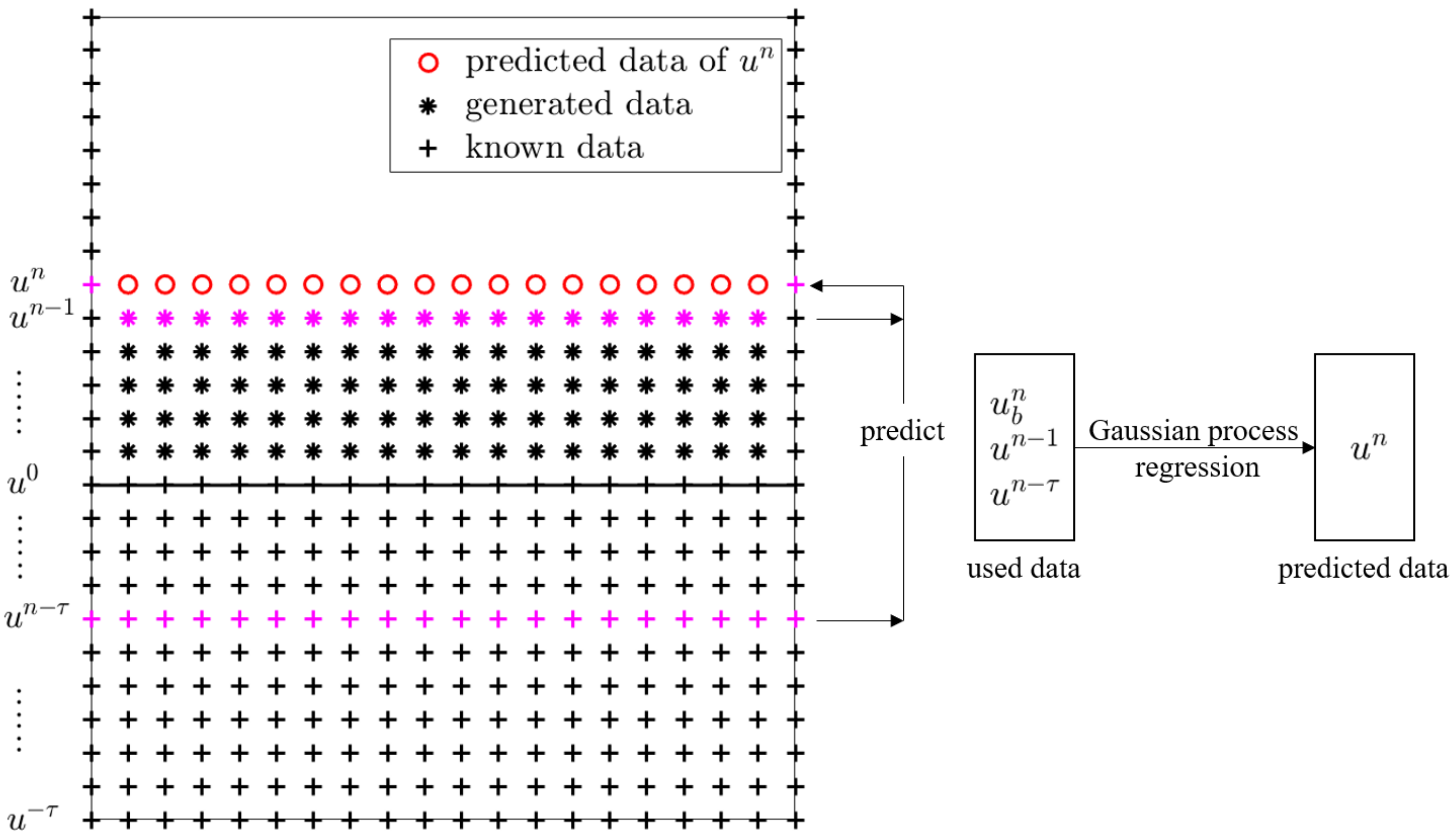
However, we exploit the Gaussian process regression to predict the next solution at each time step. Figure 1 shows the basic idea of MP-NGPs. At each iteration, the optimized hyper-parameters of the current time step are saved and deemed as initial values of the hyper-parameters in the next time step, which can significantly speed up the training process.

2.6. Processing of Fractional-Order Operators

For simplicity, we consider the following delay problem to show the processing of the fractional-order operators,

$$u_t=g(u,x)\left[\frac{{\partial }^{\alpha }}{\partial x^{\alpha }}u+\frac{{\partial }^{\beta }}{\partial x^{\beta }}u\right]+h(u,x)\frac{{\partial }^2}{\partial x^2}u(x,t-s)+f,$$

(11)

where continuous real function $u(x,t)$ is absolutely integrable in ${\mathbb{R}}^2$. Assume arbitrary-order partial derivatives of $u(x,t)$ to be continuous function and absolutely integrable in ${\mathbb{R}}^2$.

Consider the backward Euler scheme to (11) with $g(u^n,x)$ and $h(u^n,x)$ replaced by $g({\mu }^{n-1},x)$ and $h({\mu }^{n-1},x)$, respectively,

$$u^{n-1}=u^n-\Delta t·g({\mu }^{n-1},x)\frac{{\partial }^{\alpha }}{\partial x^{\alpha }}{u}^n-\Delta t·g({\mu }^{n-1},x)\frac{{\partial }^{\beta }}{\partial x^{\beta }}{u}^n-\Delta t·h({\mu }^{n-1},x)\frac{{\partial }^2}{\partial x^2}{u}^{n-\tau }-\Delta t·f^n.$$

(12)

From (12), we can obtain

$$u^{n-1}={\mathcal{L}}_x^0{u}^n+{\mathcal{L}}_x^1{u}^{n-\tau }+{\mathcal{L}}_x^2{f}^n,$$

(13)

where ${\mathcal{L}}_x^0{u}^n=u^n-\Delta t·g({\mu }^{n-1},x)\frac{{\partial }^{\alpha }}{\partial x^{\alpha }}{u}^n-\Delta t·g({\mu }^{n-1},x)\frac{{\partial }^{\beta }}{\partial x^{\beta }}{u}^n$, ${\mathcal{L}}_x^1{u}^{n-\tau }=-\Delta t·h({\mu }^{n-1},x)\frac{{\partial }^2}{\partial x^2}{u}^{n-\tau }$, and ${\mathcal{L}}_x^2{f}^n=-\Delta t·f^n$. Assume the Gaussian process prior as follows,

$$\begin{array}{c}{u}^n\left(x\right)\sim \mathcal{G}\mathcal{P}(0,k_{u,u}^{n,n}(x,x^{\prime };{\theta }_0)),\hfill \\ u^{n-\tau }\left(x\right)\sim \mathcal{G}\mathcal{P}(0,k_{u,u}^{n-\tau ,n-\tau }(x,x^{\prime };{\theta }_1)),\hfill \\ f^n\left(x\right)\sim \mathcal{G}\mathcal{P}(0,k_{f,f}^{n,n}(x,x^{\prime };{\theta }_2)).\hfill \end{array}$$

(14)

We can easily obtain the following results from Section 2.2,

$$k_{u,u}^{n-1,n-1}(x,x^{\prime })={\mathcal{L}}_x^0{\mathcal{L}}_{x^{\prime }}^0{k}_{u,u}^{n,n}(x,x^{\prime })+{\mathcal{L}}_{x^{\prime }}^1{\mathcal{L}}_x^1{k}_{u,u}^{n-\tau ,n-\tau }(x,x^{\prime })+{\mathcal{L}}_{x^{\prime }}^2{\mathcal{L}}_x^2{k}_{f,f}^{n,n}(x,x^{\prime }).$$

(15)

How to deal with the first term on the right side of (15) is one of the most important tasks. Denote $k_{in}(x,x^{\prime })={\mathcal{L}}_x^0{\mathcal{L}}_{x^{\prime }}^0{k}_{u,u}^{n,n}(x,x^{\prime })$, according to [40], the Fourier transform is carried out with respect to the spatial variable $(x,x^{\prime })$ on $k_{u,u}^{n,n}(x,x^{\prime })$ to obtain ${\widehat{k}}_{u,u}^{n,n}(\omega ,{\omega }^{\prime })$, as the excellent properties of the squared exponential covariance function $k_{u,u}^{n,n}(x,x^{\prime })$ obviously assure the feasibility of the Fourier transform of derivatives of $k_{u,u}^{n,n}(x,x^{\prime })$, according to which $k_{u,u}^{n,n}(x,x^{\prime })$ and its partial derivatives vanish for $\sqrt{x^2+{x^{\prime }}^2}\to +\infty$. Then we can obtain the following intermediate kernels:

$$\begin{array}{c}{\widehat{k}}_{u,u}^{n,n-1}(\omega ,{\omega }^{\prime })=[1-\Delta t·g^{\prime }·{(-i{\omega }^{\prime })}^{\alpha }-\Delta t·g^{\prime }·{(-i{\omega }^{\prime })}^{\beta }]{\widehat{k}}_{u,u}^{n,n}(\omega ,{\omega }^{\prime }),\hfill \\ {\widehat{k}}_{in}(\omega ,{\omega }^{\prime })=[1-\Delta t·g·{(-i\omega )}^{\alpha }-\Delta t·g·{(-i\omega )}^{\beta }][1-\Delta t·g^{\prime }·{(-i{\omega }^{\prime })}^{\alpha }-\Delta t·g^{\prime }·{(-i{\omega }^{\prime })}^{\beta }]{\widehat{k}}_{u,u}^{n,n}(\omega ,{\omega }^{\prime }),\hfill \end{array}$$

(16)

where $g=g({\mu }^{n-1}\left(x\right),x)$, $g^{\prime }=g({\mu }^{n-1}\left(x^{\prime }\right),x^{\prime })$.

At last, the inverse Fourier transform can be performed on ${\widehat{k}}_{u,u}^{n,n-1}(\omega ,{\omega }^{\prime })$ and ${\widehat{k}}_{in}(\omega ,{\omega }^{\prime })$ to obtain the kernels $k_{u,u}^{n,n-1}(x,x^{\prime })$ and $k_{in}(x,x^{\prime })$.

2.7. Numerical Tests

To verify the validity of the method proposed, three examples are provided. Firstly, we introduce the maximum absolute error $E_{\infty }$ to denote the difference between the conditional posterior mean of the prediction solution and exact solution as follows:

$$E_{\infty }\left(t^n\right)=\underset{x^{*}}{max}|u^n\left(x^{*}\right)-{\overline{u}}^n\left(x^{*}\right)|,$$

(17)

where $t^n$ is the current time, $x^{*}$ is a point random sampling from $\Omega$, $u^n\left(x^{*}\right)$ is the exact solution, and ${\overline{u}}^n\left(x^{*}\right)$ is the posterior mean of $u^n\left(x^{*}\right)$ (prediction solution).

We also introduce a notation that $max{E}_{\infty }(\Delta t)=\underset{1\le n\le N}{max}{E}_{\infty }\left(t^n\right)$, which can be seen as a measure of the prediction error under a different time step size $\Delta t$.

Then we introduce the relative spatial error ${\mathcal{L}}^2$ to represent the relative error of prediction [29],

$${\mathcal{L}}^2\left(t^n\right)=\sqrt{\sum _{x^{*}}{[u^n\left(x^{*}\right)-{\overline{u}}^n\left(x^{*}\right)]}^2}/\phantom{\sqrt{\sum _{x^{*}}{[u^n\left(x^{*}\right)-{\overline{u}}^n\left(x^{*}\right)]}^2}\sqrt{\sum _{x^{*}}{\left[u^n\left(x^{*}\right)\right]}^2}}\sqrt{\sum _{x^{*}}{\left[u^n\left(x^{*}\right)\right]}^2}.$$

(18)

Example 1.

$$\left\{\begin{array}{c}\frac{\partial u}{\partial t}=\sqrt{u}sinu·\left[(1-x)\frac{{\partial }^{\alpha }}{\partial x^{\alpha }}u(x,t)+sin\left(2\pi x\right)\frac{{\partial }^{\beta }}{\partial x^{\beta }}u(x,t)\right]+ux\frac{{\partial }^2}{\partial x^2}u(x,t-0.2)+f(x,t),(x,t)\in (0,1)\times (0,1],\hfill \\ u(0,t)=1+t^2,u(1,t)=e^{0.5}(1+t^2),t\in (0,1]\hfill \\ u(x,t)=e^{0.5x}(1+t^2),-0.2\le t\le 0,\hfill \end{array}\right.$$

(19)

where $0<\alpha ,\beta <1$. Example 1 is a fractional partial differential equation with one delay. The fractional partial derivative $\frac{{\partial }^{\alpha }}{\partial x^{\alpha }}u(x,t)$ and $\frac{{\partial }^{\beta }}{\partial x^{\beta }}u(x,t)$ is defined by (2) in the Caputo sense [40].

We fix $(\alpha ,\beta )$ to be $(0.25,0.75)$, $(0.5,0.5)$, and $(0.75,0.25)$ in turn. The exact solution of (30) is $u(x,t)=e^{0.5x}(1+t^2)$, and the inhomogeneous term $f(x,t)$ differs from each other when $(\alpha ,\beta )$ is changed,

$$f(x,t)=\left\{\begin{array}{cc}q(x,t)-\frac{\sqrt{u}sinu·(1-x)(1+t^2)}{2\Gamma \left(0.75\right)}{\int }_{-\infty }^x\frac{e^{\upsilon /2}}{{(x-\upsilon )}^{0.25}}d\upsilon -\frac{\sqrt{u}sinu·sin\left(2\pi x\right)(1+t^2)}{2\Gamma \left(0.25\right)}{\int }_{-\infty }^x\frac{e^{\upsilon /2}}{{(x-\upsilon )}^{0.75}}d\upsilon ,\hfill & (\alpha ,\beta )=(0.25,0.75),\\ q(x,t)-\frac{\sqrt{u}sinu·(1-x)(1+t^2)}{2\Gamma \left(0.5\right)}{\int }_{-\infty }^x\frac{e^{\upsilon /2}}{{(x-\upsilon )}^{0.5}}d\upsilon -\frac{\sqrt{u}sinu·sin\left(2\pi x\right)(1+t^2)}{2\Gamma \left(0.5\right)}{\int }_{-\infty }^x\frac{e^{\upsilon /2}}{{(x-\upsilon )}^{0.5}}d\upsilon ,\hfill & (\alpha ,\beta )=(0.5,0.5),\\ q(x,t)-\frac{\sqrt{u}sinu·(1-x)(1+t^2)}{2\Gamma \left(0.25\right)}{\int }_{-\infty }^x\frac{e^{\upsilon /2}}{{(x-\upsilon )}^{0.75}}d\upsilon -\frac{\sqrt{u}sinu·sin\left(2\pi x\right)(1+t^2)}{2\Gamma \left(0.75\right)}{\int }_{-\infty }^x\frac{e^{\upsilon /2}}{{(x-\upsilon )}^{0.25}}d\upsilon ,\hfill & (\alpha ,\beta )=(0.75,0.25).\end{array}\right.$$

(20)

where $q(x,t)=2e^{0.5x}t-0.25x{e}^x[1+{(t-0.2)}^2](1+t^2)$.

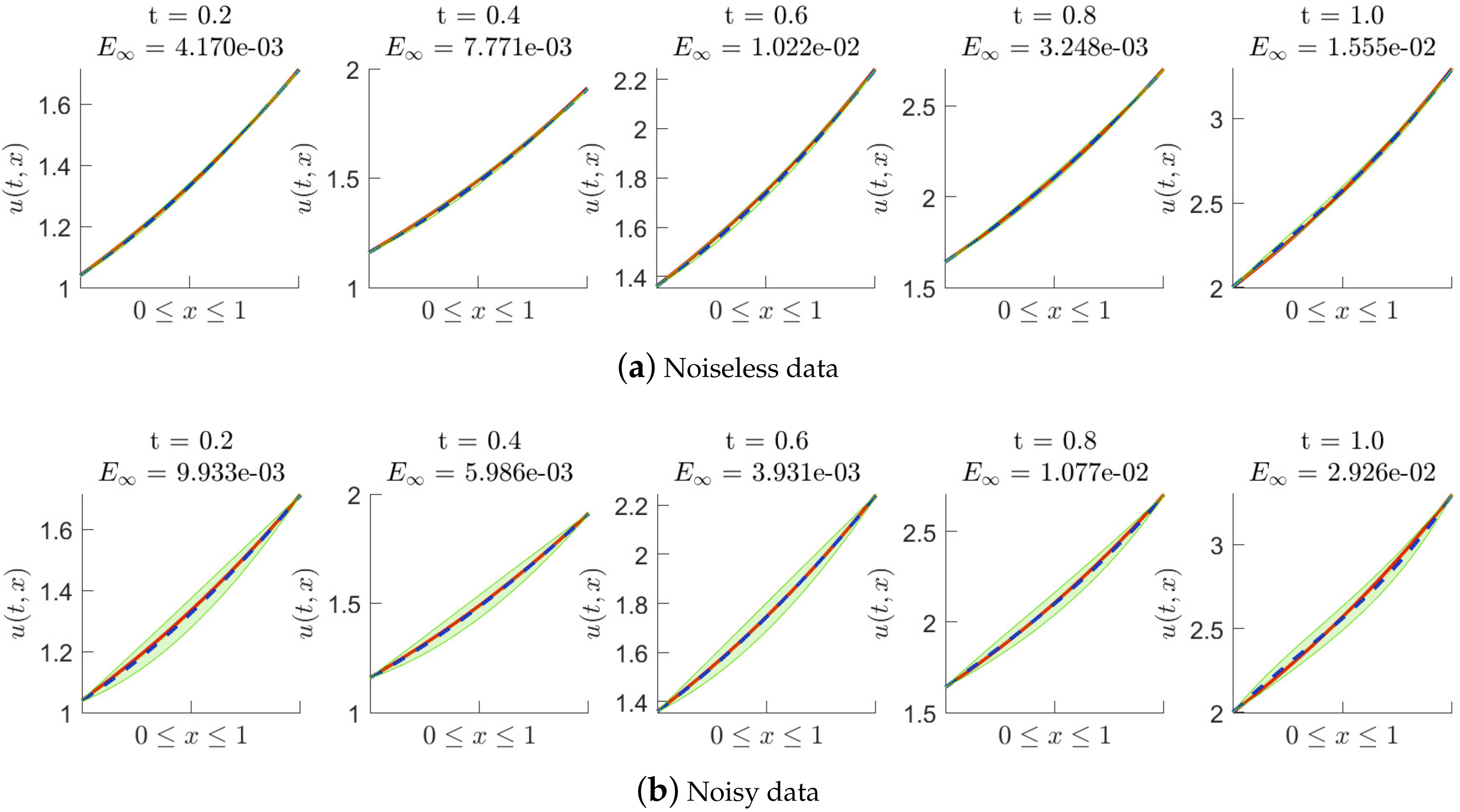
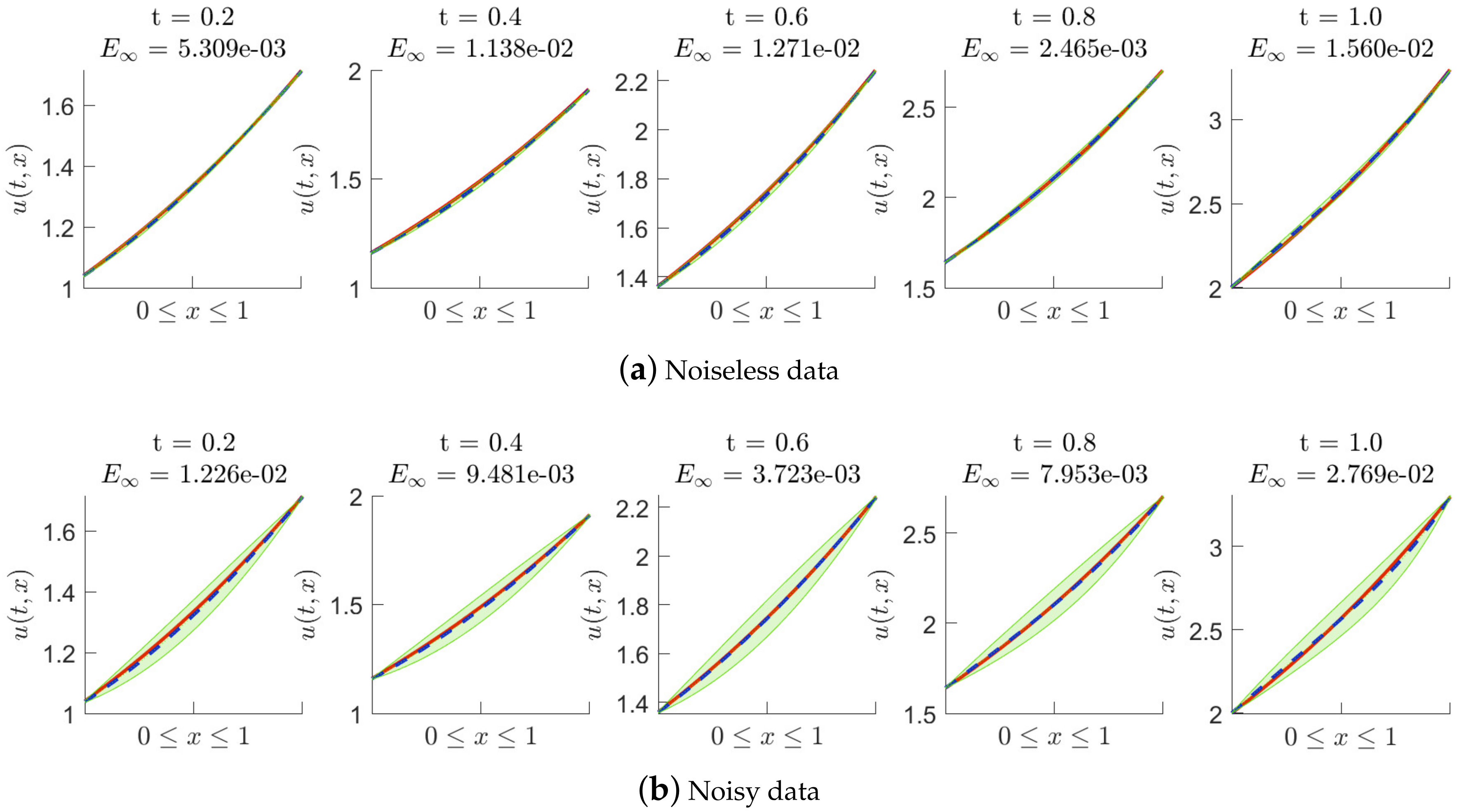
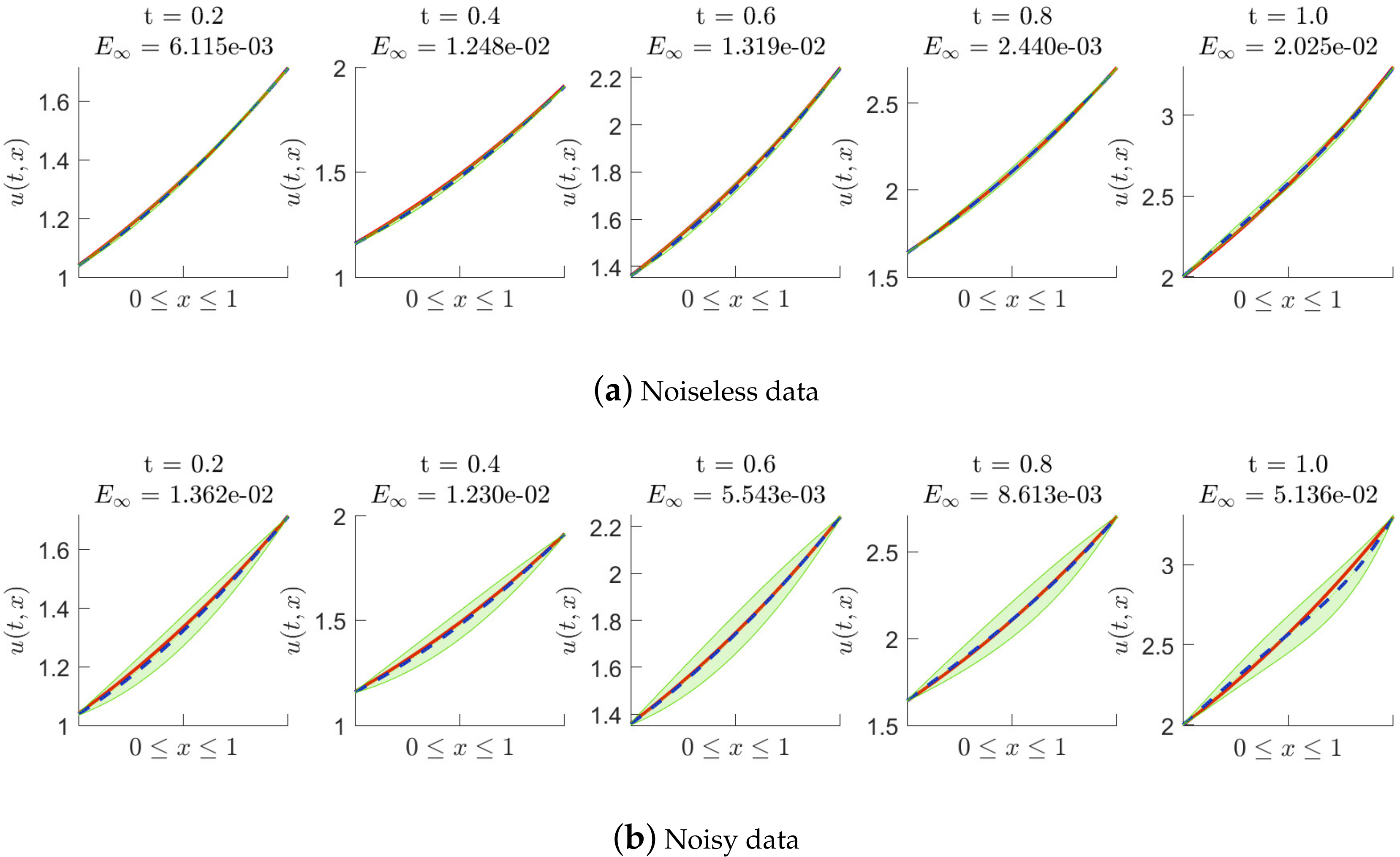
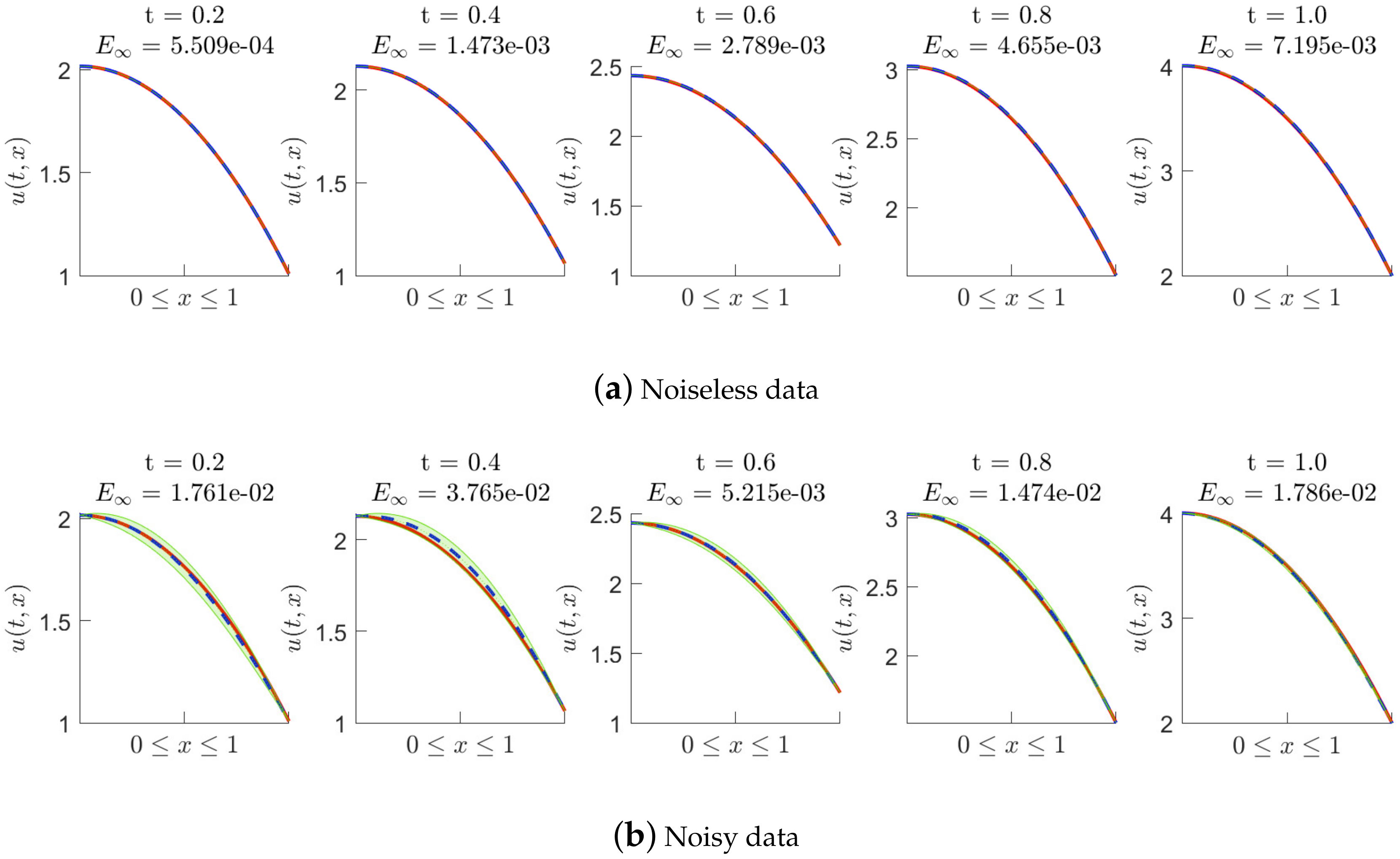
Numerical tests of solving (19) are performed with noiseless data and noisy data, respectively, where the backward Euler scheme is employed. We only add noise into the initial data ${\mathit{u}}^0$, and the additive noise of ${\mathit{u}}^0$ is ${\epsilon }_{u_0}\sim N(\mathbf{0},{0.1}^{2}I)$. Figure 2, Figure 3 and Figure 4 show the posterior distribution of the predicted solution at some time nodes, where we fix the number of initial data points (inhomogeneous term data points, artificially generated data points and delay term data points) to be 20 and $\Delta t$ to be 0.01, and take $(\alpha ,\beta )$ to be $(0.25,0.75)$, $(0.5,0.5)$, and $(0.75,0.25)$ in turn. In each of these figures, (a) presents the results of the experiments with noiseless data, and (b) presents the results of the experiments with noisy data. Moreover,

Table 1. Fractional equation of Example 1: maximum absolute error $E_{\infty }$ at some time nodes, where $\Delta t=0.01$, $(\alpha ,\beta )$ is fixed to be $(0.25,0.75)$, $(0.5,0.5)$, and $(0.75,0.25)$ in turn, and noiseless data are used.

t		$0.1$	$0.2$	$0.3$	$0.4$	$0.5$
	$(0.25,0.75)$	$4.006275\times {10}^{-3}$	$4.169644\times {10}^{-3}$	$5.313127\times {10}^{-3}$	$7.771295\times {10}^{-3}$	$1.038458\times {10}^{-2}$
$(\alpha ,\beta )$	$(0.5,0.5)$	$4.289846\times {10}^{-3}$	$5.309005\times {10}^{-3}$	$8.044738\times {10}^{-3}$	$1.138058\times {10}^{-2}$	$1.385240\times {10}^{-2}$
	$(0.75,0.25)$	$4.731742\times {10}^{-3}$	$6.114796\times {10}^{-3}$	$8.990011\times {10}^{-3}$	$1.248342\times {10}^{-2}$	$1.469581\times {10}^{-2}$
t		$0.6$	$0.7$	$0.8$	$0.9$	$1.0$
	$(0.25,0.75)$	$1.022259\times {10}^{-2}$	$7.038555\times {10}^{-3}$	$3.247575\times {10}^{-3}$	$5.014752\times {10}^{-3}$	$1.554705\times {10}^{-2}$
$(\alpha ,\beta )$	$(0.5,0.5)$	$1.270620\times {10}^{-2}$	$7.946964\times {10}^{-3}$	$2.464540\times {10}^{-3}$	$7.199783\times {10}^{-3}$	$1.560388\times {10}^{-2}$
	$(0.75,0.25)$	$1.318964\times {10}^{-2}$	$8.319928\times {10}^{-3}$	$2.440425\times {10}^{-3}$	$6.997903\times {10}^{-3}$	$2.024694\times {10}^{-2}$

shows us the maximum absolute error $E_{\infty }$ between the conditional posterior mean of the prediction solution and the exact solution at some time nodes in detail, where noiseless data is used in the experiments.

Table 2. Fractional equation of Example 1: maximum absolute error $E_{\infty }$ at some time nodes, where $\Delta t=0.01$, $(\alpha ,\beta )$ is fixed to be $(0.25,0.75)$, $(0.5,0.5)$, and $(0.75,0.25)$ in turn, and noisy data are used.

t		$0.1$	$0.2$	$0.3$	$0.4$	$0.5$
	$(0.25,0.75)$	$9.751693\times {10}^{-3}$	$9.933069\times {10}^{-3}$	$7.915402\times {10}^{-3}$	$5.985707\times {10}^{-3}$	$4.335663\times {10}^{-3}$
$(\alpha ,\beta )$	$(0.5,0.5)$	$1.037415\times {10}^{-2}$	$1.226151\times {10}^{-2}$	$1.153429\times {10}^{-2}$	$9.480904\times {10}^{-3}$	$6.599661\times {10}^{-3}$
	$(0.75,0.25)$	$1.107313\times {10}^{-2}$	$1.362223\times {10}^{-2}$	$1.362442\times {10}^{-2}$	$1.230488\times {10}^{-2}$	$9.452340\times {10}^{-3}$
t		$0.6$	$0.7$	$0.8$	$0.9$	$1.0$
	$(0.25,0.75)$	$3.930905\times {10}^{-3}$	$4.989465\times {10}^{-3}$	$1.076718\times {10}^{-2}$	$2.762690\times {10}^{-2}$	$2.925931\times {10}^{-2}$
$(\alpha ,\beta )$	$(0.5,0.5)$	$3.722859\times {10}^{-3}$	$4.222247\times {10}^{-3}$	$7.953070\times {10}^{-3}$	$2.115376\times {10}^{-2}$	$2.769300\times {10}^{-2}$
	$(0.75,0.25)$	$5.542730\times {10}^{-3}$	$3.738703\times {10}^{-3}$	$8.613066\times {10}^{-3}$	$2.476015\times {10}^{-2}$	$5.135747\times {10}^{-2}$

shows us the maximum absolute error $E_{\infty }$ at some time nodes, where noisy data are used. It is found that the method works well when solving nonlinear delay fractional equations. It is easy to observe that higher prediction accuracy is obtained by using noiseless data in experimental tests.

Example 2.

$$\left\{\begin{array}{c}\frac{\partial u}{\partial t}=(u^2+1)\left[{\int }_0^{x}u(\upsilon ,t)d\upsilon +\frac{{\partial }^{2}u(x,t)}{\partial x^2}\right]+(u+1)\frac{{\partial }^{2}u(x,t-0.2)}{\partial x^2}+f(x,t),(x,t)\in (0,1)\times (0,1],\hfill \\ u(0,t)=2(1+t^3),u(1,t)=1+t^3,t\in (0,1],\hfill \\ u(x,t)=(2-x^2)(1+t^3),-0.2\le t\le 0,\hfill \end{array}\right.$$

(21)

Example 2 is a partial integro-differential equation with one delay. The exact solution of (21) is $u(x,t)=(2-x^2)(1+t^3)$, and the inhomogeneous term is $f(x,t)=-3t^2(-2+x^2)+2[1+{(-0.2+t)}^3][1-(1+t^3)(-2+x^2)]+\frac{1}{3}(1+t^3)(6-6x+x^3)[5-4x^2+x^4+2t^3{(-2+x^2)}^2+t^6{(-2+x^2)}^2]$.

Numerical tests of solving (21) are performed with noiseless data and noisy data, respectively, where the backward Euler scheme is employed. We add noise into the initial data ${\mathit{u}}^0$ and inhomogeneous term data ${\mathit{f}}^n$ ($n=1,2,\cdots ,100$), and the additive noisy of ${\mathit{u}}^0$ and ${\mathit{f}}^n$ is ${\epsilon }_{u_0}\sim N(\mathbf{0},2^{2}I)$ and ${\epsilon }_{f_n}\sim N(\mathbf{0},4^{2}I)$, respectively. Figure 5 shows the posterior distribution of the predicted solution at different time nodes, where we fix the number of initial data points (inhomogeneous term data points, artificially generated data points and delay term data points) to be 10 and $\Delta t$ to be 0.01. In Figure 5, the five pictures on the upper side present the results of the experiments with noiseless data, and the other five pictures on the lower side present the results of the experiments with noisy data. Moreover,

Table 3. Integro-differential equation of Example 2: maximum absolute error $E_{\infty }$ at some time nodes, where $\Delta t=0.01$, where experiments are performed with noiseless data and noisy data, respectively.

t	$0.1$	$0.2$	$0.3$	$0.4$	$0.5$
$Noiselessdata$	$1.998069\times {10}^{-4}$	$5.508548\times {10}^{-4}$	$9.958003\times {10}^{-4}$	$1.473446\times {10}^{-3}$	$2.054287\times {10}^{-3}$
$Noisydata$	$1.857561\times {10}^{-2}$	$1.760902\times {10}^{-2}$	$6.577157\times {10}^{-3}$	$3.764989\times {10}^{-2}$	$3.478251\times {10}^{-2}$
t	$0.6$	$0.7$	$0.8$	$0.9$	$1.0$
$Noiselessdata$	$2.789148\times {10}^{-3}$	$3.663247\times {10}^{-3}$	$4.655392\times {10}^{-3}$	$5.852885\times {10}^{-3}$	$7.195341\times {10}^{-3}$
$Noisydata$	$5.215384\times {10}^{-3}$	$2.053576\times {10}^{-2}$	$1.473903\times {10}^{-2}$	$7.691779\times {10}^{-3}$	$1.786041\times {10}^{-2}$

shows us the maximum absolute error $E_{\infty }$ at some time nodes in detail, where noiseless data and noisy data are used in the experiments, respectively. It is found that the method works well when solving nonlinear delay integro-differential equations. It is worth noting that the computational accuracy of the prediction solution is not sensitive to noise, as the level of noise added into the data is not low.

Example 3.

$$\left\{\begin{array}{c}\frac{\partial u}{\partial t}=(usinu+x_1{x}_2{x}_3){\displaystyle \sum _{i=1}^3}\frac{{\partial }^{2}u}{\partial x_i^2}+(u^2+x_1^2)\frac{{\partial }^2}{\partial x_1{x}_2}u(x,t-0.1)+(u{x}_2{x}_3-1)\frac{{\partial }^2}{\partial x_2{x}_3}u(x,t-0.2)+f(x,t),\hfill \\ (x_1,x_2,x_3,t)\in {(0,2\pi )}^3\times (0,1],\hfill \\ u(x,t){|}_{x\in \partial {(0,2\pi )}^3}=\frac{1}{2}+\frac{sint}{10},t\in (0,1],\hfill \\ u(x,t)=(\frac{1}{2}+\frac{sint}{10}){\displaystyle \prod _{i=1}^3}(cos{x}_i+sin{x}_i),t\le 0.\hfill \end{array}\right.$$

(22)

Example 3 defines a problem with two delays and three spatial dimensions. The exact solution of (22) is $u(x_1,x_2,x_3,t)=(\frac{1}{2}+\frac{sint}{10}){\displaystyle \prod _{i=1}^3}(cos{x}_i+sin{x}_i)$, and the inhomogeneous term is

$$\begin{array}{c}f(x_1,x_2,x_3,t)=\frac{1}{10}cost(cos{x}_1+sin{x}_1)(cos{x}_2+sin{x}_2)(cos{x}_3+sin{x}_3)-\frac{1}{10}(5-sin(0.2-t))(cos{x}_1+sin{x}_1)\hfill \\ (cos{x}_2-sin{x}_2)(cos{x}_3-sin{x}_3)(-1+\frac{1}{10}{x}_2{x}_3(5+sin\left[t\right])(cos{x}_1+sin{x}_1)(cos{x}_2+sin{x}_2)(cos{x}_3+sin{x}_3))\hfill \\ -\frac{1}{10}(5-sin(0.1-t))(cos{x}_1-sin{x}_1)(cos{x}_2-sin{x}_2)(cos{x}_3+sin{x}_3)(x_1^2+\frac{1}{100}{(5+sint)}^2{(cos{x}_1+sin{x}_1)}^2\hfill \\ {(cos{x}_2+cos{x}_2)}^2{(cos{x}_3+sin{x}_3)}^2)-(\frac{1}{10}(5+sint)(cos{x}_1+sin{x}_1)(cos{x}_2+sin{x}_2)(-cos{x}_3-sin{x}_3)+\hfill \\ \frac{1}{10}(5+sint)(cos{x}_1+sin{x}_1)(-cos{x}_2-sin{x}_2)(cos{x}_3+sin{x}_3)+\frac{1}{10}(5+sint)(-cos{x}_1-sin{x}_1)(cos{x}_2+\hfill \\ sin{x}_2)(cos{x}_3+sin{x}_3)\left)\right(x_1{x}_2{x}_3+\frac{1}{10}(5+sint)(cos{x}_1+sin{x}_1)(cos{x}_2+sin{x}_2)(cos{x}_3+sin{x}_3)sin(\frac{1}{10}(5+sint)\hfill \\ (cos{x}_1+sin{x}_1)(cos{x}_2+sin{x}_2)(cos{x}_3+sin{x}_3)\left)\right).\hfill \end{array}$$

(23)

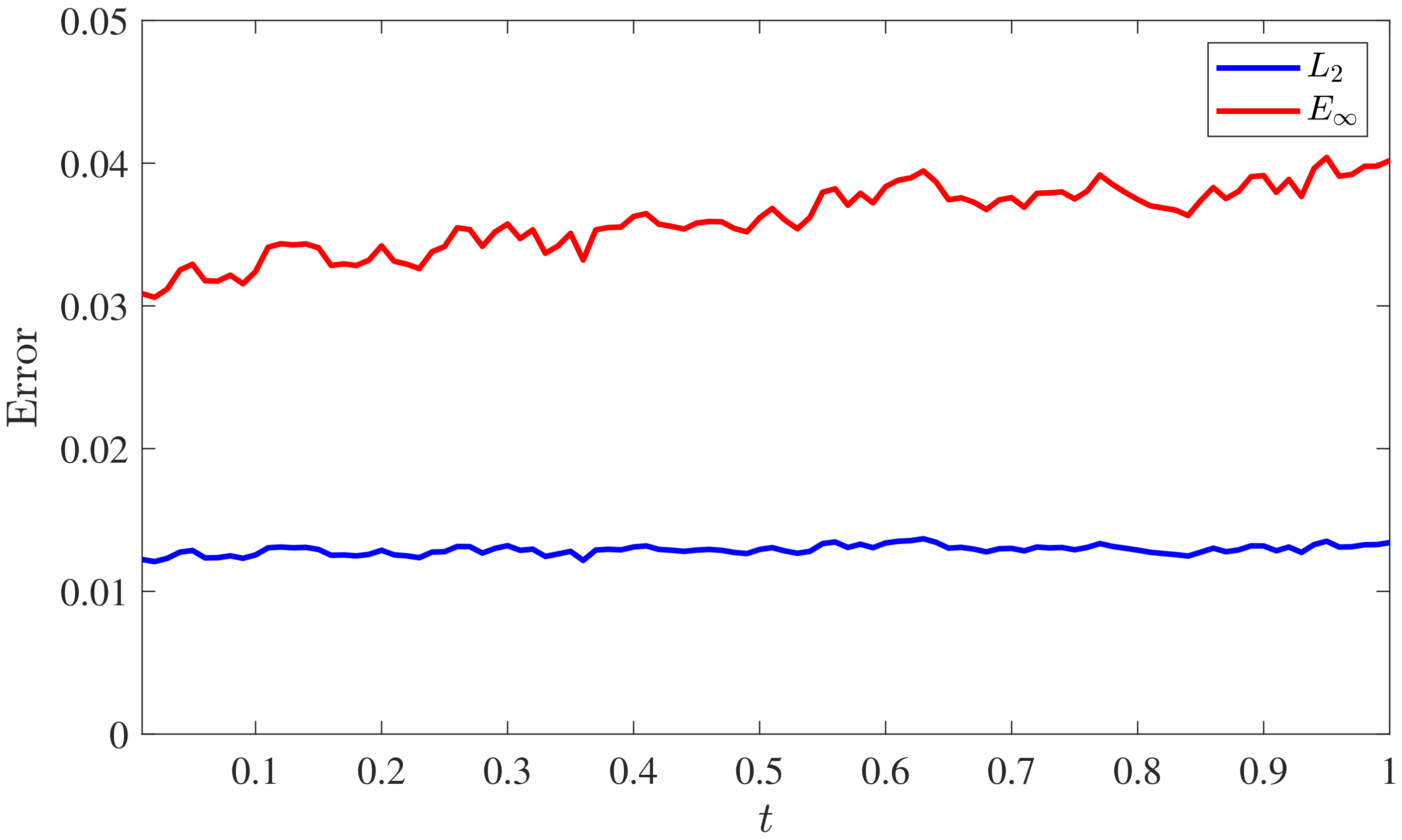
Numerical tests applying the backward Euler scheme to solve (22) will be performed with noiseless data. Figure 6 shows the relative spatial error ${\mathcal{L}}^2$ and the maximum absolute error $E_{\infty }$ with the increase in time, where we fix the number of initial data points (inhomogeneous term data points, artificially generated data points and delay term data points) to be 20 and $\Delta t$ to be 0.01. The number of training data points on each boundary line is fixed to be 5. Furthermore,

Table 4. Problem of Example 3: Relative spatial error ${\mathcal{L}}^2$ and maximum absolute error $E_{\infty }$ at some time nodes, where $\Delta t$ is fixed to be 0.01.

t	$0.1$	$0.2$	$0.3$	$0.4$	$0.5$
${\mathcal{L}}^2$	$1.255236\times {10}^{-2}$	$1.287883\times {10}^{-2}$	$1.319996\times {10}^{-2}$	$1.311049\times {10}^{-2}$	$1.293817\times {10}^{-2}$
$E_{\infty }$	$3.240473\times {10}^{-2}$	$3.420406\times {10}^{-2}$	$3.573738\times {10}^{-2}$	$3.626811\times {10}^{-2}$	$3.617718\times {10}^{-2}$
t	$0.6$	$0.7$	$0.8$	$0.9$	$1.0$
${\mathcal{L}}^2$	$1.339241\times {10}^{-2}$	$1.301079\times {10}^{-2}$	$1.289006\times {10}^{-2}$	$1.318331\times {10}^{-2}$	$1.341626\times {10}^{-2}$
$E_{\infty }$	$3.835969\times {10}^{-2}$	$3.759043\times {10}^{-2}$	$3.745873\times {10}^{-2}$	$3.913333\times {10}^{-2}$	$4.018637\times {10}^{-2}$

shows the relative spatial error ${\mathcal{L}}^2$ and the maximum absolute error $E_{\infty }$ at some time nodes in detail. According to the experimental outcome, we can conclude that the method is still effective when solving nonlinear time-dependent delay equations with high dimensions and multi-delays.

3. Runge–Kutta Methods

For the purpose of improving the accuracy of the methodology considered in Section 2, we will consider Runge–Kutta methods [47,48] based on the frame of MP-NGPs.

3.1. MP-NGPs Based on Runge–Kutta Methods

Apply Runge–Kutta methods with q stages to the first equation of (1) with appropriate approximation of nonlinear terms, and we can obtain [47]

$$\begin{array}{c}\frac{u^{n+1}-u^n}{\Delta t}={\displaystyle \sum _{j=1}^q}{b}_j\left[g({\mu }^n,\mathit{x}){\mathcal{L}}_{\mathit{x}}{u}^{n+{\varsigma }_j}+{\displaystyle \sum _{k=1}^m}{h}_k({\mu }^n,\mathit{x}){\mathcal{L}}_{\mathit{x}}^{s_k}{u}^{n+{\varsigma }_j-{\tau }_k}+f^{n+{\varsigma }_j}\right],\hfill \\ \frac{u^{n+{\varsigma }_i}-u^n}{\Delta t}={\displaystyle \sum _{j=1}^q}{a}_{ij}\left[g({\mu }^n,\mathit{x}){\mathcal{L}}_{\mathit{x}}{u}^n+{\displaystyle \sum _{k=1}^m}{h}_k({\mu }^n,\mathit{x}){\mathcal{L}}_{\mathit{x}}^{s_k}{u}^{n+{\varsigma }_j-{\tau }_k}+f^{n+{\varsigma }_j}\right],i=1,2,\cdots ,q.\hfill \end{array}$$

(24)

Reforming (24), we have

$$\begin{array}{c}{u}_{q+1}^n:=u^n=u^{n+1}-\Delta t{\displaystyle \sum _{j=1}^q}{b}_j\left[g({\mu }^n,\mathit{x}){\mathcal{L}}_{\mathit{x}}{u}^{n+{\varsigma }_j}+{\displaystyle \sum _{k=1}^m}h({\mu }^n,\mathit{x}){\mathcal{L}}_{\mathit{x}}^{s_k}{u}^{n+{\varsigma }_j-{\tau }_k}+f^{n+{\varsigma }_j}\right],\hfill \\ u_i^n:=u^n=u^{n+{\varsigma }_i}-\Delta t{\displaystyle \sum _{j=1}^q}{a}_{ij}\left[g({\mu }^n,\mathit{x}){\mathcal{L}}_{\mathit{x}}{u}^n+{\displaystyle \sum _{k=1}^m}h({\mu }^n,\mathit{x}){\mathcal{L}}_{\mathit{x}}^{s_k}{u}^{n+{\varsigma }_j-{\tau }_k}+f^{n+{\varsigma }_j}\right],i=1,2,\cdots ,q,\hfill \end{array}$$

(25)

where $u^{n+{\varsigma }_j}=u(\mathit{x},t^n+{\varsigma }_j\Delta t)$, $u^{n+{\varsigma }_j-{\tau }_k}=u(\mathit{x},t^n+{\varsigma }_j\Delta t-{\tau }_k)$, and $f^{n+{\varsigma }_j}=f(\mathit{x},t^n+{\varsigma }_j\Delta t)$. Prior assumptions are set on $u^{n+1},u^{n+{\varsigma }_i},f^{n+{\varsigma }_i},u^{n+{\varsigma }_i-{\tau }_k}(i=1,2,\cdots ,q;k=1,2,\cdots ,m)$ and Equations (25) turn into a regression problem.

Then directly write the joint distribution of $u^{n+1},u^{n+{\varsigma }_i},f^{n+{\varsigma }_i},u^{n+{\varsigma }_i-{\tau }_k},u_{q+1}^n,$$u_i^n(i=1,2,\cdots ,q;k=1,2,\cdots ,m)$. For simplicity, we introduce the Runge–Kutta methods by solving the following problem:

$$u_t=g(u,x){\mathcal{L}}_{x}u+h(u,x){\mathcal{L}}_x^{s}u(x,t-s)+f.$$

(26)

The trapezoidal rule is applied under the structure of Runge–Kutta methods to (26) with $g(u^{n+1},x)$, $h(u^{n+1},x)$, $g(u^n,x)$ and $h(u^n,x)$ replaced by $g({\mu }^n,x)$, $h({\mu }^n,x)$, $g({\mu }^n,x)$ and $h({\mu }^n,x)$, respectively. Then we have

$$\frac{u^{n+1}-u^n}{\Delta t}=\frac{1}{2}[g({\mu }^n,x){\mathcal{L}}_x{u}^{n+1}+h({\mu }^n,x){\mathcal{L}}_x^s{u}^{n+1-\tau }+f^{n+1}]+\frac{1}{2}[g({\mu }^n,x){\mathcal{L}}_x{u}^n+h({\mu }^n,x){\mathcal{L}}_x^s{u}^{n-\tau }+f^n].$$

(27)

Reforming (27), we have

$$\begin{array}{c}{u}_1^n:=u^n,\hfill \\ u_2^n:=u_3^n:=u^{n+1}-\frac{1}{2}\Delta t[g({\mu }^n,x){\mathcal{L}}_x{u}^{n+1}+h({\mu }^n,x){\mathcal{L}}_x^s{u}^{n+1-\tau }+f^{n+1}]\hfill \\ -\frac{1}{2}\Delta t[g({\mu }^n,x){\mathcal{L}}_x{u}^n+h({\mu }^n,x){\mathcal{L}}_x^s{u}^{n-\tau }+f^n].\hfill \end{array}$$

(28)

However, Equation (28) coincides with the structure of Runge–Kutta methods when $q=2,{\varsigma }_1=0,{\varsigma }_2=1,b_1=b_2=1/2,a_{11}=a_{12}=0,$ and $a_{21}=a_{22}=1/2$. Reforming (28), we obtain

$$\begin{array}{c}{u}_1^n:=u^n,\hfill \\ u_2^n:=u_3^n:={\mathcal{L}}_x^0{u}^{n+1}+{\mathcal{L}}_x^1{u}^{n+1-\tau }+{\mathcal{L}}_x^2{f}^{n+1}+{\mathcal{L}}_x^3{u}^n+{\mathcal{L}}_x^1{u}^{n-\tau }+{\mathcal{L}}_x^2{f}^n,\hfill \end{array}$$

(29)

where ${\mathcal{L}}_x^0,{\mathcal{L}}_x^1,{\mathcal{L}}_x^2$ and ${\mathcal{L}}_x^3$ are linear operators.

Assume the following prior hypotheses:

$$\begin{array}{cc}{u}^n\left(x\right)\sim \mathcal{G}\mathcal{P}(0,k_{u,u}^{n,n}(x,x^{\prime };{\theta }_1)),\hfill & u^{n+1}\left(x\right)\sim \mathcal{G}\mathcal{P}(0,k_{u,u}^{n+1,n+1}(x,x^{\prime };{\theta }_2)),\hfill \\ u^{n-\tau }\left(x\right)\sim \mathcal{G}\mathcal{P}(0,k_{u,u}^{n-\tau ,n-\tau }(x,x^{\prime };{\theta }_3)),\hfill & u^{n+1-\tau }\left(x\right)\sim \mathcal{G}\mathcal{P}(0,k_{u,u}^{n+1-\tau ,n+1-\tau }(x,x^{\prime };{\theta }_4)),\hfill \\ f^n\left(x\right)\sim \mathcal{G}\mathcal{P}(0,k_{f,f}^{n,n}(x,x^{\prime };{\theta }_5)),\hfill & f^{n+1}\left(x\right)\sim \mathcal{G}\mathcal{P}(0,k_{f,f}^{n+1,n+1}(x,x^{\prime };{\theta }_6)),\hfill \end{array}$$

(30)

to be mutually independent Gaussian processes, and assume covariance functions to be the following exponential form of (6). By the properties of the Gaussian processes, we have

$$\mathit{y}\sim \mathcal{G}\mathcal{P}(\mathbf{0},\mathit{K}),$$

where

$$\mathit{K}=\left[\begin{array}{cccccccc}{k}_{b,b}^{n+1,n+1}& k_{b,u}^{n+1,n+1-\tau }& k_{b,f}^{n+1,n+1}& k_{b,b}^{n+1,n}& k_{b,u}^{n+1,n-\tau }& k_{b,f}^{n+1,n}& k_{b,1}^{n+1,n}& k_{b,2}^{n+1,n}\\ & k_{u,u}^{n+1-\tau ,n+1-\tau }& k_{u,f}^{n+1-\tau ,n+1}& k_{u,b}^{n+1-\tau ,n}& k_{u,u}^{n+1-\tau ,n-\tau }& k_{u,f}^{n+1-\tau ,n}& k_{u,1}^{n+1-\tau ,n}& k_{u,2}^{n+1-\tau ,n}\\ & & k_{f,f}^{n+1,n+1}& k_{f,b}^{n+1,n}& k_{f,u}^{n+1,n-\tau }& k_{f,f}^{n+1,n}& k_{f,1}^{n+1,n}& k_{f,2}^{n+1,n}\\ & & & k_{b,b}^{n,n}& k_{b,u}^{n,n-\tau }& k_{b,f}^{n,n}& k_{b,1}^{n,n}& k_{b,2}^{n,n}\\ & & & & k_{u,u}^{n-\tau ,n-\tau }& k_{u,f}^{n-\tau ,n}& k_{u,1}^{n-\tau ,n}& k_{u,2}^{n-\tau ,n}\\ & & & & & k_{f,f}^{n,n}& k_{f,1}^{n,n}& k_{f,2}^{n,n}\\ & & & & & & k_{1,1}^{n,n}& k_{1,2}^{n,n}\\ & & & & & & & k_{2,2}^{n,n}\end{array}\right],$$

(31)

$$\mathit{y}=\left[\begin{array}{c}{\mathit{u}}_b^{n+1}\\ {\mathit{u}}^{n+1-\tau }\\ {\mathit{f}}^{n+1}\\ {\mathit{u}}_b^n\\ {\mathit{u}}^{n-\tau }\\ {\mathit{f}}^n\\ {\mathit{u}}_1^n\\ {\mathit{u}}_2^n\end{array}\right],\begin{array}{c}{k}_{b,b}^{n+1,n+1}=k_{u,u}^{n+1,n+1}({\mathit{x}}_b^{n+1},{\mathit{x}}_b^{n+1})+{\sigma }_{u_{n+1}}^{2}I,k_{b,b}^{n,n}=k_{u,u}^{n,n}({\mathit{x}}_b^n,{\mathit{x}}_b^n)+{\sigma }_{u_n}^{2}I,\hfill \\ k_{u,u}^{n+1-\tau ,n+1-\tau }=k_{u,u}^{n+1-\tau ,n+1-\tau }({\mathit{x}}_u^{n+1-\tau },{\mathit{x}}_u^{n+1-\tau })+{\sigma }_{u_{n+1-\tau }}^{2}I,\hfill \\ k_{u,u}^{n-\tau ,n-\tau }=k_{u,u}^{n-\tau ,n-\tau }({\mathit{x}}_u^{n-\tau },{\mathit{x}}_u^{n-\tau })+{\sigma }_{u_{n-\tau }}^{2}I,\hfill \\ k_{f,f}^{n+1,n+1}=k_{f,f}^{n+1,n+1}({\mathit{x}}_f^{n+1},{\mathit{x}}_f^{n+1})+{\sigma }_{f_{n+1}}^{2}I,k_{f,f}^{n,n}=k_{f,f}^{n,n}({\mathit{x}}_f^n,{\mathit{x}}_f^n)+{\sigma }_{f_n}^{2}I,\hfill \\ k_{b,1}^{n,n}=k_{u,u}^{n,n}({\mathit{x}}_b^n,{\mathit{x}}_u^n),k_{b,2}^{n+1,n}={\mathcal{L}}_{x^{\prime }}^0{k}_{u,u}^{n+1,n+1}({\mathit{x}}_b^{n+1},{\mathit{x}}_u^n),\hfill \\ \begin{array}{c}{k}_{u,2}^{n+1-\tau ,n}={\mathcal{L}}_{x^{\prime }}^1{k}_{u,u}^{n+1-\tau ,n+1-\tau }({\mathit{x}}_u^{n+1-\tau },{\mathit{x}}_u^n),\hfill \\ k_{f,2}^{n+1,n}={\mathcal{L}}_{x^{\prime }}^2{k}_{f,f}^{n+1,n+1}({\mathit{x}}_f^{n+1},{\mathit{x}}_u^n),\hfill \end{array}\hfill \\ k_{b,2}^{n,n}={\mathcal{L}}_{x^{\prime }}^3{k}_{u,u}^{n,n}({\mathit{x}}_b^n,{\mathit{x}}_u^n),k_{u,2}^{n-\tau ,n}={\mathcal{L}}_{x^{\prime }}^1{k}_{u,u}^{n-\tau ,n-\tau }({\mathit{x}}_u^{n-\tau },{\mathit{x}}_u^n),\hfill \\ k_{f,2}^{n,n}={\mathcal{L}}_{x^{\prime }}^2{k}_{f,f}^{n,n}({\mathit{x}}_f^n,{\mathit{x}}_u^n),k_{1,1}^{n,n}=k_{u,u}^{n,n}({\mathit{x}}_u^n,{\mathit{x}}_u^n)+{\sigma }_{u_n}^{2}I,k_{1,2}^{n,n}={\mathcal{L}}_{x^{\prime }}^3{k}_{u,u}^{n,n}({\mathit{x}}_u^n,{\mathit{x}}_u^n),\hfill \\ k_{2,2}^{n,n}={\mathcal{L}}_x^0{\mathcal{L}}_{x^{\prime }}^0{k}_{u,u}^{n+1,n+1}({\mathit{x}}_u^n,{\mathit{x}}_u^n)+{\mathcal{L}}_x^1{\mathcal{L}}_{x^{\prime }}^1{k}_{u,u}^{n+1-\tau ,n+1-\tau }({\mathit{x}}_u^n,{\mathit{x}}_u^n)\hfill \\ +{\mathcal{L}}_x^2{\mathcal{L}}_{x^{\prime }}^2{k}_{f,f}^{n+1,n+1}({\mathit{x}}_u^n,{\mathit{x}}_u^n)+{\mathcal{L}}_x^3{\mathcal{L}}_{x^{\prime }}^3{k}_{u,u}^{n,n}({\mathit{x}}_u^n,{\mathit{x}}_u^n)\hfill \\ +{\mathcal{L}}_x^1{\mathcal{L}}_{x^{\prime }}^1{k}_{u,u}^{n-\tau ,n-\tau }({\mathit{x}}_u^n,{\mathit{x}}_u^n)+{\mathcal{L}}_x^2{\mathcal{L}}_{x^{\prime }}^2{k}_{f,f}^{n,n}({\mathit{x}}_u^n,{\mathit{x}}_u^n)+{\sigma }_{u_n}^{2}I.\hfill \end{array}$$

Other kernels are assumed to be $\mathbf{0}$.

We can write the posterior distribution of the prediction $u^{n+1}\left(x_{*}^{n+1}\right)$ as follows:

$${\mathit{u}}^{n+1}\left(x_{*}^{n+1}\right)\left|\left[\begin{array}{c}{\mathit{u}}_b^{n+1}\\ {\mathit{u}}^{n+1-\tau }\\ {\mathit{f}}^{n+1}\\ {\mathit{u}}_b^n\\ {\mathit{u}}^{n-\tau }\\ {\mathit{f}}^n\\ {\mathit{u}}^n\\ {\mathit{u}}^n\end{array}\right]\right.\sim N\left(q^T{K}^{-1}\left[\begin{array}{c}{\mathit{u}}_b^{n+1}\\ {\mathit{u}}^{n+1-\tau }\\ {\mathit{f}}^{n+1}\\ {\mathit{u}}_b^n\\ {\mathit{u}}^{n-\tau }\\ {\mathit{f}}^n\\ {\mathit{u}}^n\\ {\mathit{u}}^n\end{array}\right],k_{u,u}^{n+1,n+1}(x_{*}^{n+1},x_{*}^{n+1})-{\mathit{q}}^T{\mathit{K}}^{-1}\mathit{q}\right),$$

(32)

where $q^T:=[k_{u,b}^{n+1,n+1}(x_{*}^{n+1},{\mathit{x}}_b^{n+1})$, $k_{u,u}^{n+1,n+1-\tau }(x_{*}^{n+1},{\mathit{x}}_u^{n+1-\tau })$, $k_{u,f}^{n+1,n+1}(x_{*}^{n+1},{\mathit{x}}_f^{n+1})$,

$k_{u,b}^{n+1,n}(x_{*}^{n+1},{\mathit{x}}_b^n)$, $k_{u,u}^{n+1,n-\tau }(x_{*}^{n+1},{\mathit{x}}_u^{n-\tau })$, $k_{u,f}^{n+1,n}(x_{*}^{n+1},{\mathit{x}}_f^n)$, $k_{u,u}^{n,n-{\tau }_m}(x_{*}^n,{\mathit{x}}_u^{n-{\tau }_m})$, $k_{u,1}^{n+1,n}(x_{*}^{n+1},{\mathit{x}}_u^n)$, $k_{u,2}^{n+1,n}(x_{*}^{n+1},{\mathit{x}}_u^n)]$, $k_{u,2}^{n+1,n}={\mathcal{L}}_{x^{\prime }}^0{k}_{u,u}^{n+1,n+1}(x_{*}^{n+1},{\mathit{x}}_u^n)$.

For $\{{\mathit{x}}_u^n,{\mathit{u}}^n\}$($n>0$), $\{{\mathit{x}}_u^{n-\tau },{\mathit{u}}^{n-\tau }\}$($n>\tau$) and $\{{\mathit{x}}_u^{n+1-\tau },{\mathit{u}}^{n+1-\tau }\}$($n\ge \tau$) are artificially generated data, we cannot directly use the outcome of the conditional distribution of (32) in the next time step. To propagate the uncertainty, we should marginalize ${\mathit{u}}^{n-1}$(${\mathit{u}}^{n-\tau }$, ${\mathit{u}}^{n+1-\tau }$) by employing

$$\left\{\begin{array}{c}\begin{array}{c}\begin{array}{c}{\mathit{u}}^{n+1-\eta }\left|\begin{array}{c}{\mathit{u}}_b^1,{\mathit{u}}_b^2,\cdots ,{\mathit{u}}_b^{n+1-\eta }\hfill \\ {\mathit{u}}^{1-\tau },{\mathit{u}}^{2-\tau },\cdots ,{\mathit{u}}^{n+1-\eta -\tau }\hfill \\ {\mathit{f}}^1,{\mathit{f}}^2,\cdots ,{\mathit{f}}^{n+1-\eta }\hfill \\ {\mathit{u}}_b^0,{\mathit{u}}_b^2,\cdots ,{\mathit{u}}_b^{n-\eta }\hfill \\ {\mathit{u}}^{-\tau },{\mathit{u}}^{1-\tau },\cdots ,{\mathit{u}}^{n-\eta -\tau }\hfill \\ {\mathit{f}}^0,{\mathit{f}}^1,\cdots ,{\mathit{f}}^{n-\eta }\hfill \\ {\mathit{u}}_0\hfill \end{array}\sim N\left({\mu }^{n+1-\eta },{\Sigma }^{n+1-\eta ,n+1-\eta }\right),\right.n+1-\eta \le \tau \hfill \end{array}\hfill \end{array}\\ {\mathit{u}}^{n+1-\eta }\left|\begin{array}{c}{\mathit{u}}_b^1,{\mathit{u}}_b^2,\cdots ,{\mathit{u}}_b^{n+1-\eta }\hfill \\ {\mathit{u}}^{1-\tau },{\mathit{u}}^{2-\tau },\cdots ,{\mathit{u}}^0\hfill \\ {\mathit{f}}^1,{\mathit{f}}^2,\cdots ,{\mathit{f}}^{n+1-\eta }\hfill \\ {\mathit{u}}_b^0,{\mathit{u}}_b^2,\cdots ,{\mathit{u}}_b^{n-\eta }\hfill \\ {\mathit{u}}^{-\tau },{\mathit{u}}^{1-\tau },\cdots ,{\mathit{u}}^0\hfill \\ {\mathit{f}}^0,{\mathit{f}}^1,\cdots ,{\mathit{f}}^{n-\eta }\hfill \\ {\mathit{u}}_0\hfill \end{array}\sim N\left({\mu }^{n+1-\eta },{\Sigma }^{n+1-\eta ,n+1-\eta }\right),\right.n+1-\eta >\tau \end{array}\right.$$

(33)

to get

$$\left\{\begin{array}{c}\begin{array}{c}\begin{array}{c}{u}^{n+1}\left(x_{*}^{n+1}\right)\left|\begin{array}{c}{\mathit{u}}_b^1,{\mathit{u}}_b^2,\cdots ,{\mathit{u}}_b^{n+1}\hfill \\ {\mathit{u}}^{1-\tau },{\mathit{u}}^{2-\tau },\cdots ,{\mathit{u}}^{n+1-\tau }\hfill \\ {\mathit{f}}^1,{\mathit{f}}^2,\cdots ,{\mathit{f}}^{n+1}\hfill \\ {\mathit{u}}_b^0,{\mathit{u}}_b^2,\cdots ,{\mathit{u}}_b^n\hfill \\ {\mathit{u}}^{-\tau },{\mathit{u}}^{1-\tau },\cdots ,{\mathit{u}}^{n-\tau }\hfill \\ {\mathit{f}}^0,{\mathit{f}}^1,\cdots ,{\mathit{f}}^n\hfill \\ {\mathit{u}}_0\hfill \end{array}\sim N\left({\mu }^{n+1}\left(x_{*}^{n+1}\right),{\Sigma }^{n+1,n+1}(x_{*}^{n+1},x_{*}^{n+1})\right),\right.n+1\le \tau \hfill \end{array}\hfill \end{array}\hfill \\ u^{n+1}\left(x_{*}^{n+1}\right)\left|\begin{array}{c}{\mathit{u}}_b^1,{\mathit{u}}_b^2,\cdots ,{\mathit{u}}_b^{n+1}\hfill \\ {\mathit{u}}^{1-\tau },{\mathit{u}}^{2-\tau },\cdots ,{\mathit{u}}^0\hfill \\ {\mathit{f}}^1,{\mathit{f}}^2,\cdots ,{\mathit{f}}^{n+1}\hfill \\ {\mathit{u}}_b^0,{\mathit{u}}_b^2,\cdots ,{\mathit{u}}_b^n\hfill \\ {\mathit{u}}^{-\tau },{\mathit{u}}^{1-\tau },\cdots ,{\mathit{u}}^0\hfill \\ {\mathit{f}}^0,{\mathit{f}}^1,\cdots ,{\mathit{f}}^n\hfill \\ {\mathit{u}}_0\hfill \end{array}\sim N\left({\mu }^{n+1}\left(x_{*}^{n+1}\right),{\Sigma }^{n+1,n+1}(x_{*}^{n+1},x_{*}^{n+1})\right),\right.n+1>\tau \hfill \end{array}\right.$$

(34)

where ${\mu }^{n+1}\left(x_{*}^{n+1}\right)={\mathit{q}}^T{\mathit{K}}^{-1}\left[\begin{array}{c}{\mathit{u}}_b^{n+1}\\ {\mu }^{n+1-\tau }\\ {\mathit{f}}^{n+1}\\ {\mathit{u}}_b^n\\ {\mu }^{n-\tau }\\ {\mathit{f}}^n\\ {\mu }^n\\ {\mu }^n\end{array}\right]$(if $n+1-\tau <0$, replace ${\mu }^{n+1-\tau }$ by ${\mathit{u}}^{n+1-\tau }$; if $n-\tau <0$, replace ${\mu }^{n-\tau }$ by ${\mathit{u}}^{n-\tau }$), ${\Sigma }^{n+1,n+1}(x_{*}^{n+1},x_{*}^{n+1})=k_{u,u}^{n+1,n+1}(x_{*}^{n+1},x_{*}^{n+1})-{\mathit{q}}^T{\mathit{K}}^{-1}\mathit{q}+{\mathit{q}}^T{\mathit{K}}^{-1}\mathbf{S}{\mathit{K}}^{-1}\mathit{q}$, $\mathbf{S}=diag(\mathbf{0},{\Sigma }^{n+1-\tau ,n+1-\tau },\mathbf{0},\mathbf{0},{\Sigma }^{n-\tau ,n-\tau },\mathbf{0},{\Sigma }_{2\times 2}^{n,n})$(if $n+1-\tau <0$, replace ${\Sigma }^{n+1-\tau ,n+1-\tau }$ by $\mathbf{0}$; if $n-\tau <0$, replace ${\Sigma }^{n-\tau ,n-\tau }$ by $\mathbf{0}$), and ${\Sigma }_{2\times 2}^{n,n}=\left[\begin{array}{cc}{\Sigma }^{n,n}& {\Sigma }^{n,n}\\ {\Sigma }^{n,n}& {\Sigma }^{n,n}\end{array}\right]$.

On the basis of Equation (34), we have ${\mathit{u}}^{n+1}\sim N\left({\mu }^{n+1},{\Sigma }^{n+1,n+1}\right)$, and obtain the artificial data $\{{\mathit{x}}_u^{n+1},{\mathit{u}}^{n+1}\}$ of the next step, where ${\mu }^{n+1}={\mu }^{n+1}\left({\mathit{x}}_u^{n+1}\right)$, ${\Sigma }^{n+1,n+1}={\Sigma }^{n+1,n+1}({\mathit{x}}_u^{n+1},{\mathit{x}}_u^{n+1})$.

3.2. Numerical Test for the Problem with One Delay Applying the Trapezoidal Rule

In this subsection, the method of applying the backward Euler scheme and the trapezoidal scheme is applied to solve Example 4, and numerical tests are carried out. Moreover, the impact of data noise and the amount of training data on maximum absolute error $E_{\infty }$ is investigated in this subsection.

Example 4.

$$\left\{\begin{array}{c}\frac{\partial u}{\partial t}=(u^2+sinu+2x+1)\frac{{\partial }^{2}u}{\partial x^2}+\left(ux\right)\frac{\partial }{\partial x}u(x,t-0.2)+f(x,t),(x,t)\in (0,2\pi )\times (0,1],\hfill \\ u(0,t)=e^{-t},u(2\pi ,t)=e^{-t},t\in (0,1]\hfill \\ u(x,t)=e^{-t}(cosx+sinx),t\le 0.\hfill \end{array}\right.$$

(35)

The exact solution of (35) is $u(x,t)=e^{-t}(cosx+sinx)$, and the inhomogeneous term is $f(x,t)=e^{-t}(cosx+sinx)\{2x+e^{-2t}{(cosx+sinx)}^2+sin\left[e^{-t}(cosx+sinx)\right]\}-e^{0.2-2t}xcos2x$.

Table 5. Problem of Example 4: maximum absolute error $E_{\infty }$ at five time nodes for different $\Delta t$ under the backward Euler scheme and the convergence order in time.

$\Delta \mathit{t}$	$\mathit{t}=0.2$	$\mathit{t}=0.4$	$\mathit{t}=0.6$	$\mathit{t}=0.8$	$\mathit{t}=1.0$	$max{\mathit{E}}_{\mathit{\infty }}(\Delta \mathit{t})$	$\frac{max{\mathit{E}}_{\mathit{\infty }}(2\Delta \mathit{t})}{max{\mathit{E}}_{\mathit{\infty }}(\Delta \mathit{t})}$
0.2	$5.196883\times {10}^{-2}$	$4.358087\times {10}^{-2}$	$3.277721\times {10}^{-2}$	$2.416694\times {10}^{-2}$	$1.781159\times {10}^{-2}$	$5.196883\times {10}^{-2}$	*
0.1	$2.643025\times {10}^{-2}$	$2.202658\times {10}^{-2}$	$1.643945\times {10}^{-2}$	$1.206984\times {10}^{-2}$	$8.922375\times {10}^{-3}$	$2.643025\times {10}^{-2}$	1.966
0.05	$1.354968\times {10}^{-2}$	$1.112114\times {10}^{-2}$	$8.246767\times {10}^{-3}$	$6.030003\times {10}^{-3}$	$4.610772\times {10}^{-3}$	$1.354968\times {10}^{-2}$	1.951
0.025	$6.893477\times {10}^{-3}$	$5.593641\times {10}^{-3}$	$4.121273\times {10}^{-3}$	$3.001243\times {10}^{-3}$	$2.359743\times {10}^{-3}$	$6.893477\times {10}^{-3}$	1.966
0.0125	$3.459075\times {10}^{-3}$	$2.800349\times {10}^{-3}$	$2.065297\times {10}^{-3}$	$1.507394\times {10}^{-3}$	$1.192749\times {10}^{-3}$	$3.462585\times {10}^{-3}$	1.991
0.00625	$1.753664\times {10}^{-3}$	$1.414149\times {10}^{-3}$	$1.036199\times {10}^{-3}$	$7.571422\times {10}^{-4}$	$5.988719\times {10}^{-4}$	$1.763992\times {10}^{-3}$	1.963

presents the maximum absolute error $E_{\infty }$ between the conditional posterior mean of the prediction solution and the exact solution at five time nodes for the different time step size $\Delta t$ under the backward Euler scheme, where the number of initial data points (inhomogeneous term data points, artificially generated data points and delay term data points) is fixed to be 20. It is found that the method applying the backward Euler scheme is first-order accurate in time, which is just in line with the first-order convergence property of the backward Euler scheme we applied. Since calculating the convergence order in time requires the maximum absolute error under two consecutive time steps, we omit the display of the first value in the last column of Table 5 and

Table 6. Problem of Example 4: maximum absolute error $E_{\infty }$ at five time nodes for different $\Delta t$ under the trapezoidal scheme and the convergence order in time.

$\Delta \mathit{t}$	$\mathit{t}=0.2$	$\mathit{t}=0.4$	$\mathit{t}=0.6$	$\mathit{t}=0.8$	$\mathit{t}=1.0$	$max{\mathit{E}}_{\mathit{\infty }}(\Delta \mathit{t})$	$\frac{max{\mathit{E}}_{\mathit{\infty }}(2\Delta \mathit{t})}{max{\mathit{E}}_{\mathit{\infty }}(\Delta \mathit{t})}$
0.2	$4.495057\times {10}^{-2}$	$1.990879\times {10}^{-2}$	$1.849233\times {10}^{-2}$	$1.384659\times {10}^{-2}$	$1.045600\times {10}^{-2}$	$4.495057\times {10}^{-2}$	*
0.1	$1.638529\times {10}^{-2}$	$1.275052\times {10}^{-2}$	$9.718359\times {10}^{-3}$	$7.421787\times {10}^{-3}$	$5.774761\times {10}^{-3}$	$1.747229\times {10}^{-2}$	2.573
0.05	$8.155066\times {10}^{-3}$	$6.595744\times {10}^{-3}$	$5.033765\times {10}^{-3}$	$3.856745\times {10}^{-3}$	$2.979750\times {10}^{-3}$	$8.184114\times {10}^{-3}$	2.135
0.025	$4.079031\times {10}^{-3}$	$3.340249\times {10}^{-3}$	$2.562043\times {10}^{-3}$	$1.969803\times {10}^{-3}$	$1.528144\times {10}^{-3}$	$4.088401\times {10}^{-3}$	2.002
0.0125	$2.029881\times {10}^{-3}$	$1.701985\times {10}^{-3}$	$1.300908\times {10}^{-3}$	$9.986143\times {10}^{-4}$	$7.749402\times {10}^{-4}$	$2.043320\times {10}^{-3}$	2.001
0.00625	$1.036153\times {10}^{-3}$	$8.602172\times {10}^{-4}$	$6.599498\times {10}^{-4}$	$5.096151\times {10}^{-4}$	$3.956461\times {10}^{-4}$	$1.040213\times {10}^{-3}$	1.964

.

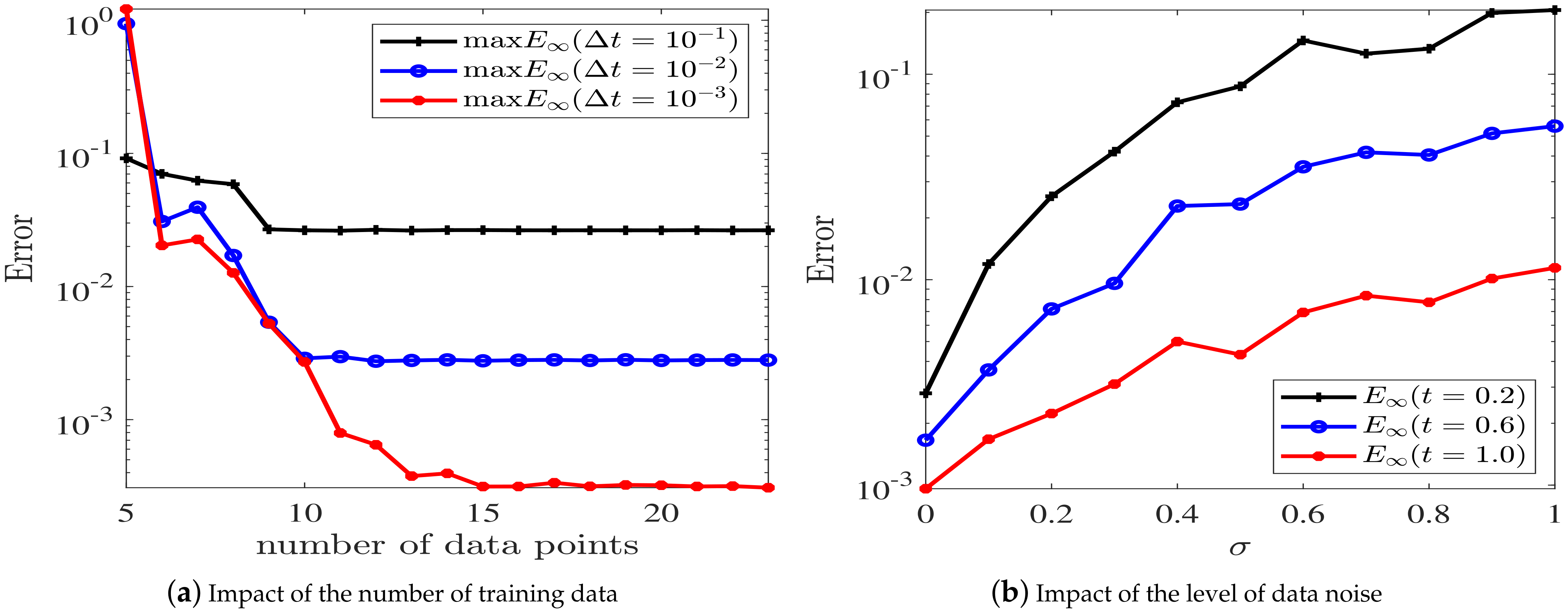
Figure 7a shows the impact of the number of initial data points (inhomogeneous term data points, artificially generated data points and delay term data points) on $max{E}_{\infty }(\Delta t)=\underset{1\le n\le N}{max}{E}_{\infty }\left(t^n\right)$, where we take $\Delta t$ as ${10}^{-1}$, ${10}^{-2}$ and ${10}^{-3}$ in turn. The results show that when $\Delta t$ is equal to ${10}^{-1}$, the prediction accuracy quickly reaches saturation with the increase in the number of training data points, but when $\Delta t$ is taken smaller, increasing the amount of training data still has the potential to improve the prediction accuracy, and the saturation behavior occurs much later.

Moreover, we investigate the impact of noise on the prediction accuracy. We add noise into the initial data ${\mathit{u}}^0$, delay term data ${\mathit{u}}^{-\tau }$ ($\tau =1,2,\cdots ,19$) and inhomogeneous term data ${\mathit{f}}^n$ ($n=1,2,\cdots ,100$) to investigate the impact of the level of the noise on the accuracy. The additive noisy of ${\mathit{u}}^0$, ${\mathit{u}}^{-\tau }$ and ${\mathit{f}}^n$ is ${\epsilon }_{u_0}\sim N(\mathbf{0},{\sigma }^{2}I)$, ${\epsilon }_{u_{-\tau }}\sim N(\mathbf{0},{\sigma }^{2}I)$ and ${\epsilon }_{f_n}\sim N(\mathbf{0},\frac{1}{4}{\sigma }^{2}I)$, respectively. Take $t=0.2,0.6,1.0$, and observe the change of $E_{\infty }$ under different $\sigma$ at these time nodes (see Figure 7b). The experiment outcome proves that the bigger $\sigma$, the lower the prediction accuracy. With the progress of the iteration, the impact of the noise on the accuracy of the current time step becomes smaller, and the accuracy gradually tends to increase, as the hyper-parameters that contain the knowledge of the considered problem are trained better and better as the iteration progress continues.

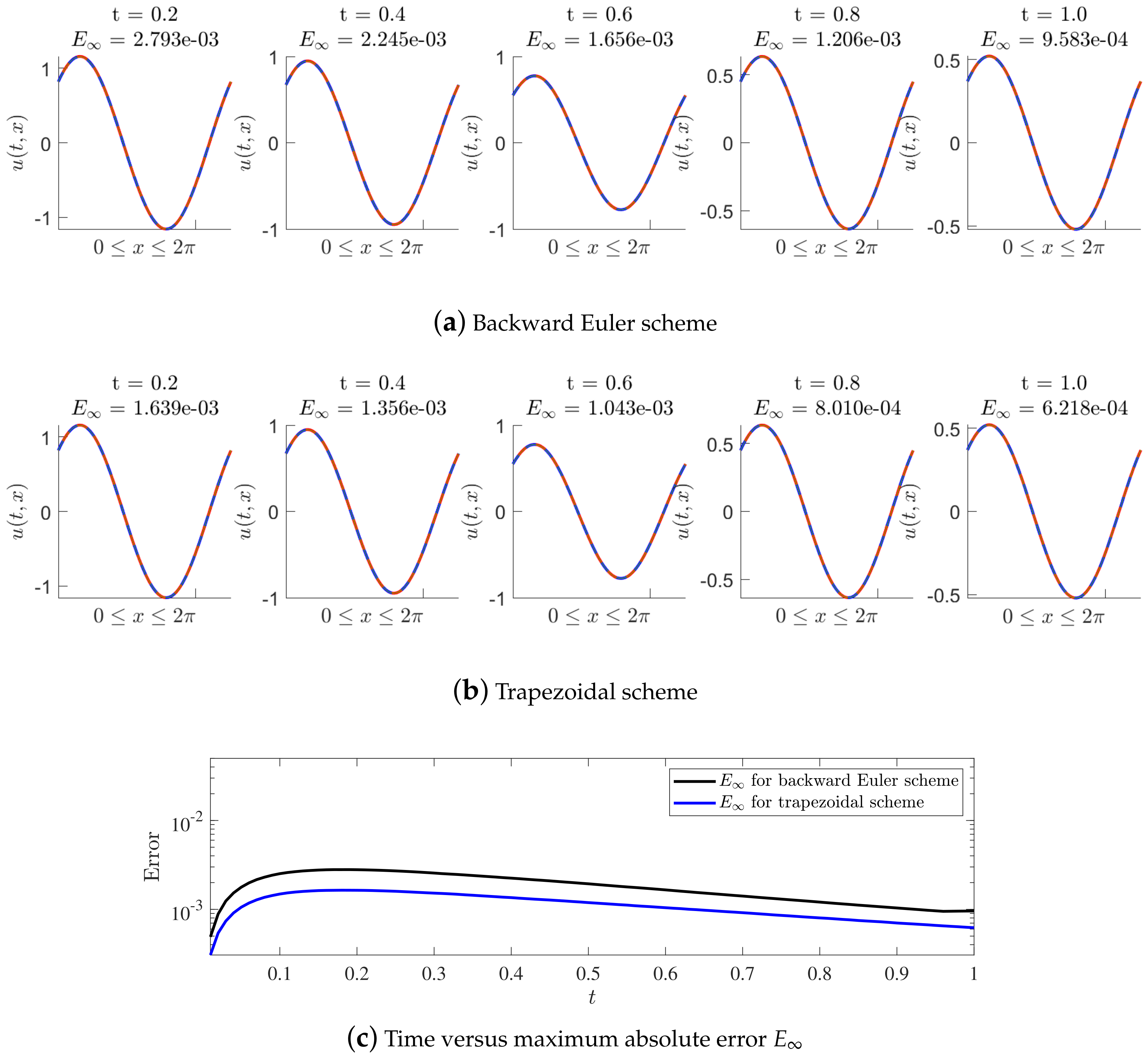
Table 6 shows the maximum absolute error $E_{\infty }$ between the conditional posterior mean of the prediction solution and the exact solution at five time nodes for the different time step size $\Delta t$ under the trapezoidal scheme, where the number of initial data points (inhomogeneous term data points, artificially generated data points and delay term data points) is fixed to be 20. It is found that the method applying the trapezoidal rule is still first-order accurate in time, which is apparently not consistent with the second-order convergence property of the trapezoidal rule. Therefore, we can conclude from these results that the convergence rate of MP-NGPs using Runge–Kutta methods is also the first-order. Fortunately, the accuracy of the method applying the trapezoidal scheme (Runge–Kutta methods) does exceed the backward Euler scheme when other experimental conditions are fixed, which means that applying the Runge–Kutta methods on MP-NGPs is still very useful when the current accuracy is not satisfying. The results of Figure 8 also prove that the Runge–Kutta methods do exceed the backward Euler scheme in prediction accuracy.

4. Processing of Neumann and Mixed Boundary Conditions

In the above sections, we did not mention the processing of other boundary conditions, except Dirichlet boundary conditions. This section will introduce how to solve two-dimensional PDEs with Neumann or mixed boundary conditions. That is, the spatial vector $\mathit{x}$ is a one-dimensional variable.

As everyone knows, Dirichlet, Neumann and mixed boundary conditions have the following general form, respectively, in the problem (1) of two dimensions:

$$u(\mathrm{lb},t)={\varphi }_1\left(t\right),u(\mathrm{ub},t)={\varphi }_2\left(t\right),0<t\le \mathrm{T},$$

(36)

$${\left.\left[\frac{\partial u}{\partial x}\right]\right|}_{x=\mathrm{lb}}={\psi }_1\left(t\right),{\left.\left[\frac{\partial u}{\partial x}\right]\right|}_{x=\mathrm{ub}}={\psi }_2\left(t\right),0<t\le \mathrm{T},$$

(37)

$${\left.\left[{\lambda }_{11}\left(t\right)\frac{\partial u}{\partial x}+{\lambda }_{12}\left(t\right)u\right]\right|}_{x=\mathrm{lb}}={\xi }_1\left(t\right),{\left.\left[{\lambda }_{21}\left(t\right)\frac{\partial u}{\partial x}+{\lambda }_{22}\left(t\right)u\right]\right|}_{x=\mathrm{ub}}={\xi }_2\left(t\right),0<t\le \mathrm{T},$$

(38)

where ${\varphi }_1\left(t\right),{\varphi }_2\left(t\right)$, ${\psi }_1\left(t\right),{\psi }_2\left(t\right)$, ${\lambda }_{11}\left(t\right),{\lambda }_{12}\left(t\right),{\lambda }_{21}\left(t\right),{\lambda }_{22}\left(t\right),{\xi }_1\left(t\right),{\xi }_2\left(t\right)$ are given functions.

In order to avoid the repetitive introduction, we will focus on the processing of Neumann and mixed boundary conditions in this section.

4.1. Neumann Boundary Conditions

For the Neumann boundary conditions (37), introduce $v^n=\frac{\partial u^n}{\partial x}$, where $v^n\left(x\right)=v(x,t^n)=\frac{\partial u(x,t^n)}{\partial x}$. Note ${\mathcal{L}}_x^v{u}^n=\frac{\partial u^n}{\partial x}$, and ${\mathcal{L}}_x^v$ is a linear operator.

Return to the problem (1), then we can get $\mathit{y}\sim \mathcal{G}\mathcal{P}(\mathbf{0},\mathit{K})$, where

$$\mathit{y}=\left[\begin{array}{c}{\mathit{v}}_b^n\\ {\mathit{u}}^{n-{\tau }_1}\\ ⋮\\ {\mathit{u}}^{n-{\tau }_m}\\ {\mathit{f}}^n\\ {\mathit{u}}^{n-1}\end{array}\right],\mathit{K}=\left[\begin{array}{cccccc}{k}_{v,v}^{n,n}& k_{v,u}^{n,n-{\tau }_1}& \cdots & k_{v,u}^{n,n-{\tau }_m}& k_{v,f}^{n,n}& k_{v,u}^{n,n-1}\\ & k_{u,u}^{n-{\tau }_1,n-{\tau }_1}& \cdots & k_{u,u}^{n-{\tau }_1,n-{\tau }_m}& k_{u,f}^{n-{\tau }_1,n}& k_{u,u}^{n-{\tau }_1,n-1}\\ & & \ddots & ⋮& ⋮& ⋮\\ & & & k_{u,u}^{n-{\tau }_m,n-{\tau }_m}& k_{u,f}^{n-{\tau }_m,n}& k_{u,u}^{n-{\tau }_m,n-1}\\ & & & & k_{f,f}^{n,n}& k_{f,u}^{n,n-1}\\ & & & & & k_{u,u}^{n-1,n-1}\end{array}\right],$$

$$\begin{array}{c}{k}_{v,v}^{n,n}={\mathcal{L}}_x^v{\mathcal{L}}_{x^{\prime }}^v{k}_{u,u}^{n,n}({\mathit{x}}_b^n,{\mathit{x}}_b^n)+{\sigma }_{v_n}^{2}I,k_{f,f}^{n,n}=k_{f,f}^{n,n}({\mathit{x}}_f^n,{\mathit{x}}_f^n)+{\sigma }_{f_n}^{2}I,{\mathit{x}}_b^n=\{\mathrm{lb},\mathrm{ub}\},\hfill \\ k_{u,u}^{n-{\tau }_i,n-{\tau }_i}=k_{u,u}^{n-{\tau }_i,n-{\tau }_i}({\mathit{x}}_u^{n-{\tau }_i},{\mathit{x}}_u^{n-{\tau }_i})+{\sigma }_{u_{n-{\tau }_i}}^{2}I,i=1,2,\cdots ,m,\hfill \\ k_{v,u}^{n,n-{\tau }_i}=k_{v,u}^{n,n-{\tau }_i}({\mathit{x}}_b^n,{\mathit{x}}_u^{n-{\tau }_i})=\mathbf{0},k_{u,f}^{n-{\tau }_i,n}=k_{u,f}^{n-{\tau }_i,n}({\mathit{x}}_u^{n-{\tau }_i},{\mathit{x}}_f^n)=\mathbf{0},i=1,2,\cdots ,m,\hfill \\ k_{v,f}^{n,n}=k_{u,f}^{n,n}({\mathit{x}}_b^n,{\mathit{x}}_f^n)=\mathbf{0},\hfill \\ k_{u,u}^{n-{\tau }_l,n-{\tau }_k}=k_{u,u}^{n-{\tau }_l,n-{\tau }_k}({\mathit{x}}_u^{n-{\tau }_l},{\mathit{x}}_u^{n-{\tau }_k})=\mathbf{0},l=1,2,\cdots ,m,k=1,2,\cdots ,m,\hfill \\ k_{v,u}^{n,n-1}={\mathcal{L}}_x^v{\mathcal{L}}_{x^{\prime }}^0{k}_{u,u}^{n,n}({\mathit{x}}_b^n,{\mathit{x}}_u^{n-1}),k_{u,u}^{n-{\tau }_i,n-1}={\mathcal{L}}_{x^{\prime }}^i{k}_{u,u}^{n-{\tau }_i,n-{\tau }_i}({\mathit{x}}_u^{n-{\tau }_i},{\mathit{x}}_u^{n-1}),i=1,2,\cdots ,m,\hfill \\ k_{f,u}^{n,n-1}={\mathcal{L}}_{x^{\prime }}^{m+1}{k}_{f,f}^{n,n}({\mathit{x}}_f^n,{\mathit{x}}_u^{n-1}),\hfill \\ k_{u,u}^{n-1,n-1}={\mathcal{L}}_x^0{\mathcal{L}}_{x^{\prime }}^0{k}_{u,u}^{n,n}({\mathit{x}}_u^{n-1},{\mathit{x}}_u^{n-1})+{\displaystyle \sum _{i=1}^m}{\mathcal{L}}_x^i{\mathcal{L}}_{x^{\prime }}^i{k}_{u,u}^{n-{\tau }_i,n-{\tau }_i}({\mathit{x}}_u^{n-1},{\mathit{x}}_u^{n-1})\hfill \\ +{\mathcal{L}}_x^{m+1}{\mathcal{L}}_{x^{\prime }}^{m+1}{k}_{f,f}^{n,n}({\mathit{x}}_u^{n-1},{\mathit{x}}_u^{n-1})+{\sigma }_{u_{n-1}}^{2}I.\hfill \end{array}$$

where ${\mathit{v}}_b^n=v({\mathit{x}}_b^n,t^n)+{\epsilon }_{v_n}$, ${\epsilon }_{v_n}\sim N(\mathbf{0},{\sigma }_{v_n}^{2}I)$. The additive noise ${\epsilon }_{v_n}$ is assumed to be independent of other noise.

By (5), train the hyper-parameters $\left\{{\theta }_j\right|j=0,1,\cdots ,m+1\}$ by minimizing NLML (39),

$$-logp\left(\mathit{y}\right|{\mathit{x}}_b^n,{\mathit{x}}_u^{n-{\tau }_1},\cdots ,{\mathit{x}}_u^{n-{\tau }_m},{\mathit{x}}_f^n,{\mathit{x}}_u^{n-1},{\theta }_0,\cdots ,{\theta }_{m+1})=\frac{1}{2}log\left|\mathit{K}\right|+\frac{1}{2}{\mathit{y}}^T{\mathit{K}}^{-1}\mathit{y}+\frac{N}{2}log2\pi ,$$

(39)

After the training part, the posterior distribution of $u^n\left(x_{*}^n\right)$ can be directly written as

$$u^n\left(x_{*}^n\right)\left|\left[\begin{array}{c}{\mathit{v}}_b^n\\ {\mathit{u}}^{n-{\tau }_1}\\ ⋮\\ {\mathit{u}}^{n-{\tau }_m}\\ {\mathit{f}}^n\\ {\mathit{u}}^{n-1}\end{array}\right]\right.\sim N\left({\mathit{q}}^T{\mathit{K}}^{-1}\left[\begin{array}{c}{\mathit{v}}_b^n\\ {\mathit{u}}^{n-{\tau }_1}\\ ⋮\\ {\mathit{u}}^{n-{\tau }_m}\\ {\mathit{f}}^n\\ {\mathit{u}}^{n-1}\end{array}\right],k_{u,u}^{n,n}(x_{*}^n,x_{*}^n)-{\mathit{q}}^T{\mathit{K}}^{-1}\mathit{q}\right),$$

(40)

where ${\mathit{q}}^T:=[k_{u,v}^{n,n}(x_{*}^n,{\mathit{x}}_b^n),k_{u,u}^{n,n-{\tau }_1}(x_{*}^n,{\mathit{x}}_u^{n-{\tau }_1}),\cdots ,k_{u,u}^{n,n-{\tau }_m}(x_{*}^n,{\mathit{x}}_u^{n-{\tau }_m}),k_{u,f}^{n,n}(x_{*}^n,{\mathit{x}}_f^n)$,

$k_{u,u}^{n,n-1}(x_{*}^n,{\mathit{x}}_u^{n-1})]$, $k_{u,v}^{n,n}(x_{*}^n,{\mathit{x}}_b^n)={\mathcal{L}}_{x^{\prime }}^v{k}_{u,u}^{n,n}(x_{*}^n,{\mathit{x}}_b^n)$.

On the basis of Section 2.4, in order to accurately propagate the uncertainty, marginalize ${\mathit{u}}^{n-1}$ (and perhaps ${\mathit{u}}^{n-{\tau }_j}$, when $n>{\tau }_j$) by employing (assume ${\tau }_q<n-\eta \le {\tau }_{q+1}$)

$${\mathit{u}}^{n-\eta }\left|\begin{array}{c}{\mathit{v}}_b^1,{\mathit{v}}_b^2,\cdots ,{\mathit{v}}_b^{n-\eta }\\ {\mathit{u}}^{1-{\tau }_1},{\mathit{u}}^{2-{\tau }_1},\cdots ,{\mathit{u}}^0\\ ⋮\\ {\mathit{u}}^{1-{\tau }_q},{\mathit{u}}^{2-{\tau }_q},\cdots ,{\mathit{u}}^0\\ {\mathit{u}}^{1-{\tau }_{q+1}},{\mathit{u}}^{2-{\tau }_{q+1}},\cdots ,{\mathit{u}}^{n-\eta -{\tau }_{q+1}}\\ ⋮\\ {\mathit{u}}^{1-{\tau }_m},{\mathit{u}}^{2-{\tau }_m},\cdots ,{\mathit{u}}^{n-\eta -{\tau }_m}\\ {\mathit{f}}^1,{\mathit{f}}^2,\cdots ,{\mathit{f}}^{n-\eta }\\ {\mathit{u}}^0\end{array}\sim N\left({\mu }^{n-\eta },{\Sigma }^{n-\eta ,n-\eta }\right),\right.$$

(41)

to obtain (assume ${\tau }_p<n\le {\tau }_{p+1}$)

$$u^n\left(x_{*}^n\right)\left|\begin{array}{c}{\mathit{v}}_b^1,{\mathit{v}}_b^2,\cdots ,{\mathit{v}}_b^n\\ {\mathit{u}}^{1-{\tau }_1},{\mathit{u}}^{2-{\tau }_1},\cdots ,{\mathit{u}}^0\\ ⋮\\ {\mathit{u}}^{1-{\tau }_p},{\mathit{u}}^{2-{\tau }_p},\cdots ,{\mathit{u}}^0\\ {\mathit{u}}^{1-{\tau }_{p+1}},{\mathit{u}}^{2-{\tau }_{p+1}},\cdots ,{\mathit{u}}^{n-{\tau }_{p+1}}\\ ⋮\\ {\mathit{u}}^{1-{\tau }_m},{\mathit{u}}^{2-{\tau }_m},\cdots ,{\mathit{u}}^{n-{\tau }_m}\\ {\mathit{f}}^1,{\mathit{f}}^2,\cdots ,{\mathit{f}}^n\\ {\mathit{u}}^0\end{array}\sim N\left({\mu }^n\left(x_{*}^n\right),{\Sigma }^{n,n}(x_{*}^n,x_{*}^n)\right),\right.$$

(42)

where ${\mu }^n\left(x_{*}^n\right)={\mathit{q}}^T{\mathit{K}}^{-1}\left[\begin{array}{c}{\mathit{v}}_b^n\\ {\mu }^{n-{\tau }_1}\\ ⋮\\ {\mu }^{n-{\tau }_p}\\ {\mathit{u}}^{n-{\tau }_{p+1}}\\ ⋮\\ {\mathit{u}}^{n-{\tau }_m}\\ {\mathit{f}}^n\\ {\mu }^{n-1}\end{array}\right]$, ${\Sigma }^{n,n}(x_{*}^n,x_{*}^n)=k_{u,u}^{n,n}(x_{*}^n,x_{*}^n)-{\mathit{q}}^T{\mathit{K}}^{-1}\mathit{q}+{\mathit{q}}^T{\mathit{K}}^{-1}\mathbf{S}{\mathit{K}}^{-1}\mathit{q}$, and $\mathbf{S}=diag(\mathbf{0},{\Sigma }^{n-{\tau }_1,n-{\tau }_1},\cdots ,{\Sigma }^{n-{\tau }_p,n-{\tau }_p},\cdots ,\mathbf{0},\cdots ,{\Sigma }^{n-1,n-1})$.

By the posterior distribution (42), obtain the simplified form ${\mathit{u}}^n\sim N\left({\mu }^n,{\Sigma }^{n,n}\right)$, and then obtain the artificial data $\{{\mathit{x}}_u^n,{\mathit{u}}^n\}$ of the next time step, where ${\mu }^n={\mu }^n\left({\mathit{x}}_u^n\right)$, and ${\Sigma }^{n,n}={\Sigma }^{n,n}({\mathit{x}}_u^n,{\mathit{x}}_u^n)$.

Let us return to the problem (11) in Section 2.6, and the operator ${\mathcal{L}}_x^0$ contains fractional-order operators. Then $k_{v,u}^{n,n-1}(x,x^{\prime })$ can be obtained by performing the inverse Fourier transform on ${\widehat{k}}_{v,u}^{n,n-1}(\omega ,{\omega }^{\prime })$, where

$${\widehat{k}}_{v,u}^{n,n-1}(\omega ,{\omega }^{\prime })=(-i\omega )[1-\Delta t·g^{\prime }·{(-i{\omega }^{\prime })}^{\alpha }-\Delta t·g^{\prime }·{(-i{\omega }^{\prime })}^{\beta }]{\widehat{k}}_{u,u}^{n,n}(\omega ,{\omega }^{\prime }).$$

(43)

4.2. Mixed Boundary Conditions

For the mixed boundary conditions (38), the processing of boundary information is more complicated. Introduce $w_1^n={\lambda }_{11}^n\frac{\partial u^n}{\partial x}+{\lambda }_{12}^n{u}^n$, $w_2^n={\lambda }_{21}^n\frac{\partial u^n}{\partial x}+{\lambda }_{22}^n{u}^n$, where ${\lambda }_{11}^n={\lambda }_{11}\left(t^n\right)$, ${\lambda }_{12}^n={\lambda }_{12}\left(t^n\right)$, ${\lambda }_{21}^n={\lambda }_{21}\left(t^n\right)$, ${\lambda }_{22}^n={\lambda }_{22}\left(t^n\right)$. Note ${\mathcal{L}}_x^{w_1}{u}^n={\lambda }_{11}^n\frac{\partial u^n}{\partial x}+{\lambda }_{12}^n{u}^n$, ${\mathcal{L}}_x^{w_2}{u}^n={\lambda }_{21}^n\frac{\partial u^n}{\partial x}+{\lambda }_{22}^n{u}^n$, where ${\mathcal{L}}_x^{w_1}$ and ${\mathcal{L}}_x^{w_2}$ are linear operators.

Return to the problem (1), then we can obtain $\mathit{y}\sim \mathcal{G}\mathcal{P}(\mathbf{0},\mathit{K})$, where

$$\mathit{y}=\left[\begin{array}{c}{w}_{1,\mathrm{lb}}^n\\ w_{2,\mathrm{ub}}^n\\ {\mathit{u}}^{n-{\tau }_1}\\ ⋮\\ {\mathit{u}}^{n-{\tau }_m}\\ {\mathit{f}}^n\\ {\mathit{u}}^{n-1}\end{array}\right],\mathit{K}=\left[\begin{array}{ccccccc}{k}_{w_1,w_1}^{n,n}& k_{w_1,w_2}^{n,n}& k_{w_1,u}^{n,n-{\tau }_1}& \cdots & k_{w_1,u}^{n,n-{\tau }_m}& k_{w_1,f}^{n,n}& k_{w_1,u}^{n,n-1}\\ & k_{w_2,w_2}^{n,n}& k_{w_2,u}^{n,n-{\tau }_1}& \cdots & k_{w_2,u}^{n,n-{\tau }_m}& k_{w_2,f}^{n,n}& k_{w_2,u}^{n,n-1}\\ & & k_{u,u}^{n-{\tau }_1,n-{\tau }_1}& \cdots & k_{u,u}^{n-{\tau }_1,n-{\tau }_m}& k_{u,f}^{n-{\tau }_1,n}& k_{u,u}^{n-{\tau }_1,n-1}\\ & & & \ddots & ⋮& ⋮& ⋮\\ & & & & k_{u,u}^{n-{\tau }_m,n-{\tau }_m}& k_{u,f}^{n-{\tau }_m,n}& k_{u,u}^{n-{\tau }_m,n-1}\\ & & & & & k_{f,f}^{n,n}& k_{f,u}^{n,n-1}\\ & & & & & & k_{u,u}^{n-1,n-1}\end{array}\right],$$

(44)

$$\begin{array}{c}{k}_{w_1,w_1}^{n,n}={\mathcal{L}}_x^{w_1}{\mathcal{L}}_{x^{\prime }}^{w_1}{k}_{u,u}^{n,n}(\mathrm{lb},\mathrm{lb})+{\sigma }_{w_{1,n}}^2,k_{w_2,w_2}^{n,n}={\mathcal{L}}_x^{w_2}{\mathcal{L}}_{x^{\prime }}^{w_2}{k}_{u,u}^{n,n}(\mathrm{ub},\mathrm{ub})+{\sigma }_{w_{2,n}}^2,\hfill \\ k_{f,f}^{n,n}=k_{f,f}^{n,n}({\mathit{x}}_f^n,{\mathit{x}}_f^n)+{\sigma }_{f_n}^{2}I,k_{u,u}^{n-{\tau }_i,n-{\tau }_i}=k_{u,u}^{n-{\tau }_i,n-{\tau }_i}({\mathit{x}}_u^{n-{\tau }_i},{\mathit{x}}_u^{n-{\tau }_i})+{\sigma }_{u_{n-{\tau }_i}}^{2}I,i=1,2,\cdots ,m,\hfill \\ k_{w_1,u}^{n,n-{\tau }_i}=k_{w_1,u}^{n,n-{\tau }_i}(\mathrm{lb},{\mathit{x}}_u^{n-{\tau }_i})=\mathbf{0},k_{w_2,u}^{n,n-{\tau }_i}=k_{w_2,u}^{n,n-{\tau }_i}(\mathrm{ub},{\mathit{x}}_u^{n-{\tau }_i})=\mathbf{0},k_{u,f}^{n-{\tau }_i,n}=k_{u,f}^{n-{\tau }_i,n}({\mathit{x}}_u^{n-{\tau }_i},{\mathit{x}}_f^n)=\mathbf{0},i=1,2,\cdots ,m,\hfill \\ k_{w_1,f}^{n,n}=k_{w_1,f}^{n,n}(\mathrm{lb},{\mathit{x}}_f^n)=\mathbf{0},k_{w_2,f}^{n,n}=k_{w_2,f}^{n,n}(\mathrm{ub},{\mathit{x}}_f^n)=\mathbf{0},\hfill \\ k_{u,u}^{n-{\tau }_l,n-{\tau }_k}=k_{u,u}^{n-{\tau }_l,n-{\tau }_k}({\mathit{x}}_u^{n-{\tau }_l},{\mathit{x}}_u^{n-{\tau }_k})=\mathbf{0},l=1,2,\cdots ,m,k=1,2,\cdots ,m,\hfill \\ k_{w_1,u}^{n,n-1}={\mathcal{L}}_x^{w_1}{\mathcal{L}}_{x^{\prime }}^0{k}_{u,u}^{n,n}(\mathrm{lb},{\mathit{x}}_u^{n-1}),k_{w_2,u}^{n,n-1}={\mathcal{L}}_x^{w_2}{\mathcal{L}}_{x^{\prime }}^0{k}_{u,u}^{n,n}(\mathrm{ub},{\mathit{x}}_u^{n-1}),k_{w_1,w_2}^{n,n}={\mathcal{L}}_x^{w_1}{\mathcal{L}}_{x^{\prime }}^{w_2}{k}_{u,u}^{n,n}(\mathrm{lb},\mathrm{ub}),\hfill \\ k_{u,u}^{n-{\tau }_i,n-1}={\mathcal{L}}_{x^{\prime }}^i{k}_{u,u}^{n-{\tau }_i,n-{\tau }_i}({\mathit{x}}_u^{n-{\tau }_i},{\mathit{x}}_u^{n-1}),i=1,2,\cdots ,m,\hfill \\ k_{f,u}^{n,n-1}={\mathcal{L}}_{x^{\prime }}^{m+1}{k}_{f,f}^{n,n}({\mathit{x}}_f^n,{\mathit{x}}_u^{n-1}),\hfill \\ k_{u,u}^{n-1,n-1}={\mathcal{L}}_x^0{\mathcal{L}}_{x^{\prime }}^0{k}_{u,u}^{n,n}({\mathit{x}}_u^{n-1},{\mathit{x}}_u^{n-1})+{\displaystyle \sum _{i=1}^m}{\mathcal{L}}_x^i{\mathcal{L}}_{x^{\prime }}^i{k}_{u,u}^{n-{\tau }_i,n-{\tau }_i}({\mathit{x}}_u^{n-1},{\mathit{x}}_u^{n-1})+{\mathcal{L}}_x^{m+1}{\mathcal{L}}_{x^{\prime }}^{m+1}{k}_{f,f}^{n,n}({\mathit{x}}_u^{n-1},{\mathit{x}}_u^{n-1})+{\sigma }_{u_{n-1}}^{2}I.\hfill \end{array}$$

(45)

where $w_{1,\mathrm{lb}}^n=w_1(\mathrm{lb},t^n)+{\epsilon }_{w_{1,n}}$, ${\epsilon }_{w_{1,n}}\sim N(0,{\sigma }_{w_{1,n}}^2)$, $w_{2,\mathrm{ub}}^n=w_2(\mathrm{ub},t^n)+{\epsilon }_{w_{2,n}}$, ${\epsilon }_{w_{2,n}}\sim N(0,{\sigma }_{w_{2,n}}^2)$. The additive noise ${\epsilon }_{w_{1,n}}$ and ${\epsilon }_{w_{2,n}}$ are assumed to be independent of other noise.

By (5), train the hyper-parameters $\left\{{\theta }_j\right|j=0,1,\cdots ,m+1\}$ by minimizing NLML (46),

$$-logp\left(\mathit{y}\right|{\mathit{x}}_b^n,{\mathit{x}}_u^{n-{\tau }_1},\cdots ,{\mathit{x}}_u^{n-{\tau }_m},{\mathit{x}}_f^n,{\mathit{x}}_u^{n-1},{\theta }_0,\cdots ,{\theta }_{m+1})=\frac{1}{2}log\left|\mathit{K}\right|+\frac{1}{2}{\mathit{y}}^T{\mathit{K}}^{-1}\mathit{y}+\frac{N}{2}log2\pi ,$$

(46)

After the training part, the posterior distribution of $u^n\left(x_{*}^n\right)$ can be directly written as

$$u^n\left(x_{*}^n\right)\left|\left[\begin{array}{c}{w}_{1,\mathrm{lb}}^n\\ w_{2,\mathrm{ub}}^n\\ {\mathit{u}}^{n-{\tau }_1}\\ ⋮\\ {\mathit{u}}^{n-{\tau }_m}\\ {\mathit{f}}^n\\ {\mathit{u}}^{n-1}\end{array}\right]\right.\sim N\left({\mathit{q}}^T{\mathit{K}}^{-1}\left[\begin{array}{c}{w}_{1,\mathrm{lb}}^n\\ w_{2,\mathrm{ub}}^n\\ {\mathit{u}}^{n-{\tau }_1}\\ ⋮\\ {\mathit{u}}^{n-{\tau }_m}\\ {\mathit{f}}^n\\ {\mathit{u}}^{n-1}\end{array}\right],k_{u,u}^{n,n}(x_{*}^n,x_{*}^n)-{\mathit{q}}^T{\mathit{K}}^{-1}\mathit{q}\right),$$

(47)

where ${\mathit{q}}^T=[k_{u,w_1}^{n,n}(x_{*}^n,\mathrm{lb}),k_{u,w_2}^{n,n}(x_{*}^n,\mathrm{ub}),k_{u,u}^{n,n-{\tau }_1}(x_{*}^n,{\mathit{x}}_u^{n-{\tau }_1}),\cdots ,k_{u,u}^{n,n-{\tau }_m}(x_{*}^n,{\mathit{x}}_u^{n-{\tau }_m}),$$k_{u,f}^{n,n}(x_{*}^n,{\mathit{x}}_f^n),k_{u,u}^{n,n-1}(x_{*}^n,{\mathit{x}}_u^{n-1})]$, $k_{u,w_1}^{n,n}(x_{*}^n,\mathrm{lb})={\mathcal{L}}_{x^{\prime }}^{w_1}{k}_{u,u}^{n,n}(x_{*}^n,\mathrm{lb}),k_{u,w_2}^{n,n}(x_{*}^n,\mathrm{ub})={\mathcal{L}}_{x^{\prime }}^{w_2}{k}_{u,u}^{n,n}(x_{*}^n,\mathrm{ub})$.

By Section 2.4, in order to accurately propagate the uncertainty, marginalize ${\mathit{u}}^{n-1}$ (and perhaps ${\mathit{u}}^{n-{\tau }_j}$, when $n>{\tau }_j$) by employing (assume ${\tau }_q<n-\eta \le {\tau }_{q+1}$)

$${\mathit{u}}^{n-\eta }\left|\begin{array}{c}{w}_{1,\mathrm{lb}}^1,w_{1,\mathrm{lb}}^2,\cdots ,w_{1,\mathrm{lb}}^{n-\eta }\\ w_{2,\mathrm{ub}}^1,w_{2,\mathrm{ub}}^2,\cdots ,w_{2,\mathrm{ub}}^{n-\eta }\\ {\mathit{u}}^{1-{\tau }_1},{\mathit{u}}^{2-{\tau }_1},\cdots ,{\mathit{u}}^0\\ ⋮\\ {\mathit{u}}^{1-{\tau }_q},{\mathit{u}}^{2-{\tau }_q},\cdots ,{\mathit{u}}^0\\ {\mathit{u}}^{1-{\tau }_{q+1}},{\mathit{u}}^{2-{\tau }_{q+1}},\cdots ,{\mathit{u}}^{n-\eta -{\tau }_{q+1}}\\ ⋮\\ {\mathit{u}}^{1-{\tau }_m},{\mathit{u}}^{2-{\tau }_m},\cdots ,{\mathit{u}}^{n-\eta -{\tau }_m}\\ {\mathit{f}}^1,{\mathit{f}}^2,\cdots ,{\mathit{f}}^{n-\eta }\\ {\mathit{u}}^0\end{array}\sim N\left({\mu }^{n-\eta },{\Sigma }^{n-\eta ,n-\eta }\right),\right.$$

(48)

to obtain (assume ${\tau }_p<n\le {\tau }_{p+1}$)

$$u^n\left(x_{*}^n\right)\left|\begin{array}{c}{w}_{1,\mathrm{lb}}^1,w_{1,\mathrm{lb}}^2,\cdots ,w_{1,\mathrm{lb}}^n\\ w_{2,\mathrm{ub}}^1,w_{2,\mathrm{ub}}^2,\cdots ,w_{2,\mathrm{ub}}^n\\ {\mathit{u}}^{1-{\tau }_1},{\mathit{u}}^{2-{\tau }_1},\cdots ,{\mathit{u}}^0\\ ⋮\\ {\mathit{u}}^{1-{\tau }_p},{\mathit{u}}^{2-{\tau }_p},\cdots ,{\mathit{u}}^0\\ {\mathit{u}}^{1-{\tau }_{p+1}},{\mathit{u}}^{2-{\tau }_{p+1}},\cdots ,{\mathit{u}}^{n-{\tau }_{p+1}}\\ ⋮\\ {\mathit{u}}^{1-{\tau }_m},{\mathit{u}}^{2-{\tau }_m},\cdots ,{\mathit{u}}^{n-{\tau }_m}\\ {\mathit{f}}^1,{\mathit{f}}^2,\cdots ,{\mathit{f}}^n\\ {\mathit{u}}^0\end{array}\sim N\left({\mu }^n\left(x_{*}^n\right),{\Sigma }^{n,n}(x_{*}^n,x_{*}^n)\right),\right.$$

(49)

where ${\mu }^n\left(x_{*}^n\right)={\mathit{q}}^T{\mathit{K}}^{-1}\left[\begin{array}{c}{w}_{1,lb}^n\\ w_{2,ub}^n\\ {\mu }^{n-{\tau }_1}\\ ⋮\\ {\mu }^{n-{\tau }_p}\\ {\mathit{u}}^{n-{\tau }_{p+1}}\\ ⋮\\ {\mathit{u}}^{n-{\tau }_m}\\ {\mathit{f}}^n\\ {\mu }^{n-1}\end{array}\right]$, ${\Sigma }^{n,n}(x_{*}^n,x_{*}^n)=k_{u,u}^{n,n}(x_{*}^n,x_{*}^n)-{\mathit{q}}^T{\mathit{K}}^{-1}\mathit{q}+{\mathit{q}}^T{\mathit{K}}^{-1}\mathbf{S}{\mathit{K}}^{-1}\mathit{q}$, and $\mathbf{S}=diag(\mathbf{0},{\Sigma }^{n-{\tau }_1,n-{\tau }_1},\cdots ,{\Sigma }^{n-{\tau }_p,n-{\tau }_p},\cdots ,\mathbf{0},\cdots ,{\Sigma }^{n-1,n-1})$.

On the basis of the posterior distribution (49), obtain the simplified form ${\mathit{u}}^n\sim N\left({\mu }^n,{\Sigma }^{n,n}\right)$, and then obtain the artificial data $\{{\mathit{x}}_u^n,{\mathit{u}}^n\}$ of the next time step, where ${\mu }^n={\mu }^n\left({\mathit{x}}_u^n\right)$, and ${\Sigma }^{n,n}={\Sigma }^{n,n}({\mathit{x}}_u^n,{\mathit{x}}_u^n)$.

Return to problem (11) in Section 2.6, and the operator ${\mathcal{L}}_x^0$ contains fractional-order operators. Then $k_{w_1,u}^{n,n-1}(x,x^{\prime })$ and $k_{w_2,u}^{n,n-1}(x,x^{\prime })$ can be obtained by performing the inverse Fourier transform on ${\widehat{k}}_{w_1,u}^{n,n-1}(\omega ,{\omega }^{\prime })$ and ${\widehat{k}}_{w_2,u}^{n,n-1}(\omega ,{\omega }^{\prime })$, respectively, where

$$\begin{array}{c}{\widehat{k}}_{w_1,u}^{n,n-1}(\omega ,{\omega }^{\prime })=[{\lambda }_{11}^n(-i\omega )+{\lambda }_{12}^n][1-\Delta t·g^{\prime }·{(-i{\omega }^{\prime })}^{\alpha }-\Delta t·g^{\prime }·{(-i{\omega }^{\prime })}^{\beta }]{\widehat{k}}_{u,u}^{n,n}(\omega ,{\omega }^{\prime }),\hfill \\ {\widehat{k}}_{w_2,u}^{n,n-1}(\omega ,{\omega }^{\prime })=[{\lambda }_{21}^n(-i\omega )+{\lambda }_{22}^n][1-\Delta t·g^{\prime }·{(-i{\omega }^{\prime })}^{\alpha }-\Delta t·g^{\prime }·{(-i{\omega }^{\prime })}^{\beta }]{\widehat{k}}_{u,u}^{n,n}(\omega ,{\omega }^{\prime }).\hfill \end{array}$$

(50)

4.3. Numerical Tests for a Problem with Two Delays and Different Types of Boundary Conditions

In this subsection, we will solve a nonlinear PDE with two delays, and Dirichlet, Neumann and mixed boundary conditions will be considered in this PDE, in turn.

Example 5.

$$\left\{\begin{array}{c}\frac{\partial u}{\partial t}=(u+1)\frac{{\partial }^{2}u}{\partial x^2}+sinu\frac{\partial }{\partial x}u(x,t-0.1)+cosu\frac{\partial }{\partial x}u(x,t-0.2)+f(x,t),(x,t)\in (0,2\pi )\times (0,1],\hfill \\ u(x,t)=(1+t^2)(\frac{x}{2\pi }+sinx),-0.2\le t\le 0,\hfill \end{array}\right.$$

(51)

Example 5 is a nonlinear PDE with two delays. The exact solution of (51) is $u(x,t)=(1+t^2)(\frac{x}{2\pi }+sinx)$, and the inhomogeneous term is $f(x,t)=\frac{1}{2\pi }(-((1+{(-0.2+t)}^2)(1+2\pi cosx)cos\left((1+t^2)(\frac{x}{2\pi }+sinx)\right))+2t(x+2\pi sinx)+(1+t^2)sinx(2\pi +(1+t^2)(x+2\pi sinx))-(1+{(-0.1+t)}^2)(1+2\pi cosx)sin\left((1+t^2)(\frac{x}{2\pi }+sinx)\right))$. The Dirichlet, Neumann and mixed boundary conditions of Example 5 are as follows:

$$u(0,t)=0,u(2\pi ,t)=1+t^2,0<t\le 1,$$

(52)

$${\left.\left[\frac{\partial u}{\partial x}\right]\right|}_{x=0}=(\frac{1}{2\pi }+1)(1+t^2),{\left.\left[\frac{\partial u}{\partial x}\right]\right|}_{x=2\pi }=(\frac{1}{2\pi }+1)(1+t^2),0<t\le 1.$$

(53)

$$\begin{array}{c}{\left.\left[(4+t)\frac{\partial u}{\partial x}+(1+t^2)u\right]\right|}_{x=0}=(\frac{1}{2\pi }+1)(4+t)(1+t^2),0<t\le 1,\hfill \\ {\left.\left[{(1+t)}^2\frac{\partial u}{\partial x}+(3+2sint)u\right]\right|}_{x=2\pi }=[(\frac{1}{2\pi }+1){(1+t)}^2+(3+2sint)](1+t^2),0<t\le 1.\hfill \end{array}$$

(54)

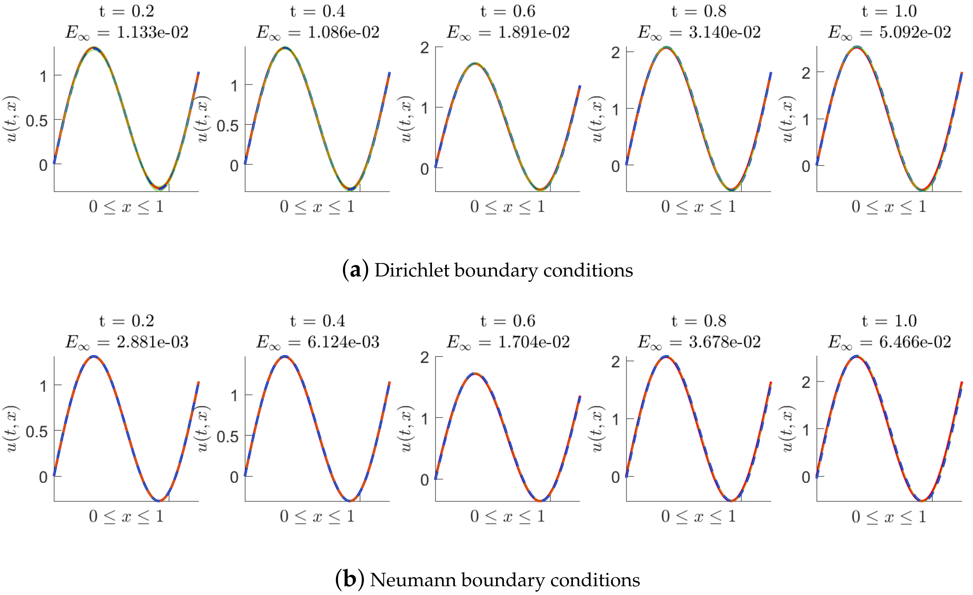
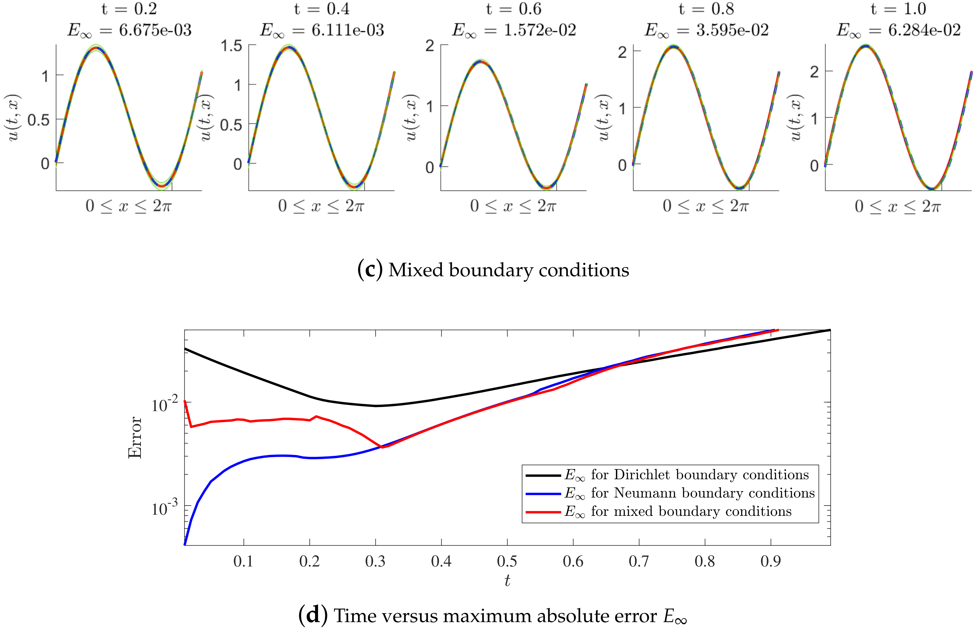
Numerical tests of solving (51) will be performed with noiseless data. Figure 9 shows the posterior distribution of the predicted solution at different time nodes, where we fix the number of initial data points (inhomogeneous term data points, artificially generated data points and delay term data points) to be 10 and fix $\Delta t$ to be 0.01. Figure 9a–c presents the results of the experiments with Dirichlet, Neumann and mixed boundary conditions, respectively, and Figure 9d shows the maximum absolute error $E_{\infty }$ with the increase in time. Moreover,

Table 7. Example 5: Maximum absolute error $E_{\infty }$ at some time nodes, where $\Delta t=0.01$, where Dirichlet, Neumann and mixed boundary conditions are used, respectively.

t	$0.1$	$0.2$	$0.3$	$0.4$	$0.5$
$Dirichlet$	$1.933660\times {10}^{-2}$	$1.133342\times {10}^{-2}$	$9.185798\times {10}^{-3}$	$1.085891\times {10}^{-2}$	$1.424333\times {10}^{-2}$
$Neumann$	$2.687072\times {10}^{-3}$	$2.880986\times {10}^{-3}$	$3.562039\times {10}^{-3}$	$6.123954\times {10}^{-3}$	$1.009985\times {10}^{-2}$
$Mixed$	$6.755766\times {10}^{-3}$	$6.675441\times {10}^{-3}$	$3.984626\times {10}^{-3}$	$6.110999\times {10}^{-3}$	$9.978279\times {10}^{-3}$
t	$0.6$	$0.7$	$0.8$	$0.9$	$1.0$
$Dirichlet$	$1.890978\times {10}^{-2}$	$2.444410\times {10}^{-2}$	$3.139654\times {10}^{-2}$	$4.025414\times {10}^{-2}$	$5.092472\times {10}^{-2}$
$Neumann$	$1.704219\times {10}^{-2}$	$2.634275\times {10}^{-2}$	$3.677554\times {10}^{-2}$	$4.920981\times {10}^{-2}$	$6.465664\times {10}^{-2}$
$Mixed$	$1.571632\times {10}^{-2}$	$2.541023\times {10}^{-2}$	$3.595499\times {10}^{-2}$	$4.830915\times {10}^{-2}$	$6.284298\times {10}^{-2}$

shows us the maximum absolute error $E_{\infty }$ at some time nodes in detail, where Dirichlet, Neumann and mixed boundary conditions are both considered. It is found that the method based on MP-NGPs works well when solving nonlinear delay PDEs with Dirichlet, Neumann or mixed boundary conditions. The prediction accuracy under different types of boundary conditions is close to each other.

5. Processing of Wave Equations

So as to prove the efficiency of MP-NGPs, we give the processing of another type of time-dependent PDEs, wave equations,

$$\left\{\begin{array}{c}\frac{{\partial }^{2}u(x,t)}{\partial t^2}=\frac{{\partial }^{2}u(x,t)}{\partial x^2}+\frac{\partial u(x,t-s)}{\partial x}+f(x,t),lb<x<ub,0<t\le \mathrm{T},\hfill \\ u(lb,t)={\varphi }_1\left(t\right),u(ub,t)={\varphi }_2\left(t\right),0<t\le \mathrm{T},\hfill \\ u(x,t)=\psi (x,t),lb\le x\le ub,-s\le t\le 0,\hfill \\ \frac{\partial u}{\partial t}(x,0)=\phi \left(x\right),lb\le x\le ub,\hfill \end{array}\right.$$

(55)

where ${\varphi }_1\left(t\right)$, ${\varphi }_2\left(t\right)$, $\psi (x,t)$, and $\phi \left(x\right)$ are given functions. Apparently, delay terms and inhomogeneous terms are also considered in the wave equations.

We will give two methods of how to solve wave equations by the algorithm of MP-NGPs.

5.1. Second Order Central Difference Scheme

The first method is to apply a second-order central difference scheme of second-order derivatives on the first Equation of (55) to discretize the temporal variable:

$$\frac{u^{n-1}+u^{n+1}-2u^n}{\Delta t^2}=\frac{{\partial }^2}{\partial x^2}{u}^n+\frac{\partial }{\partial x}{u}^{n-\tau }+f^n,$$

(56)

where $n=0,1,\cdots ,N-1$, $N=\mathrm{T}/\Delta t$, $u^n=u(x,t^n)$, $u^{n-\tau }=u(x,t^n-s)$, $\tau =s/\Delta t$, $f^n=f(x,t^n)$.

Rearrange (56) to obtain

$$u^{n+1}=2u^n+\Delta t^2\frac{{\partial }^2}{\partial x^2}{u}^n-u^{n-1}+\Delta t^2\frac{\partial }{\partial x}{u}^{n-\tau }+\Delta t^2{f}^n.$$

(57)

Obviously, the scheme (56) is a multi-steps method, while the backward Euler scheme is a one-step method. Then introduce notations that ${\mathcal{L}}_x^0{u}^n=2u^n+\Delta t^2\frac{{\partial }^2}{\partial x^2}{u}^n$, ${\mathcal{L}}_x^1{u}^{n-1}=-u^{n-1}$, ${\mathcal{L}}_x^2{u}^{n-\tau }=\Delta t^2\frac{\partial }{\partial x}{u}^{n-\tau }$ and ${\mathcal{L}}_x^3{f}^n=\Delta t^2{f}^n$. So, we can obtain the simplified equation

$$u^{n+1}={\mathcal{L}}_x^0{u}^n+{\mathcal{L}}_x^1{u}^{n-1}+{\mathcal{L}}_x^2{u}^{n-\tau }+{\mathcal{L}}_x^3{f}^n.$$

(58)

Assume the Gaussian process prior as follows:

$$\begin{array}{c}{u}^n\left(x\right)\sim \mathcal{G}\mathcal{P}(0,k_{u,u}^{n,n}(x,x^{\prime };{\theta }_0)),\hfill \\ u^{n-1}\left(x\right)\sim \mathcal{G}\mathcal{P}(0,k_{u,u}^{n-1,n-1}(x,x^{\prime };{\theta }_1)),\hfill \\ u^{n-\tau }\left(x\right)\sim \mathcal{G}\mathcal{P}(0,k_{u,u}^{n-\tau ,n-\tau }(x,x^{\prime };{\theta }_2)),\hfill \\ f^n\left(x\right)\sim \mathcal{G}\mathcal{P}(0,k_{f,f}^{n,n}(x,x^{\prime };{\theta }_3)).\hfill \end{array}$$

(59)

According to the properties of Gaussian processes, then we can obtain $\mathit{y}\sim \mathcal{G}\mathcal{P}(\mathbf{0},\mathit{K})$, where

$$\mathit{y}=\left[\begin{array}{c}{\mathit{u}}^n\\ {\mathit{u}}^{n-1}\\ {\mathit{u}}^{n-\tau }\\ {\mathit{f}}^n\\ {\mathit{u}}_b^{n+1}\end{array}\right],\mathit{K}=\left[\begin{array}{ccccc}{k}_{u,u}^{n,n}& k_{u,u}^{n,n-1}& k_{u,u}^{n,n-\tau }& k_{u,f}^{n,n}& k_{u,b}^{n,n+1}\\ & k_{u,u}^{n-1,n-1}& k_{u,u}^{n-1,n-\tau }& k_{u,f}^{n-1,n}& k_{u,b}^{n-1,n+1}\\ & & k_{u,u}^{n-\tau ,n-\tau }& k_{u,f}^{n-\tau ,n}& k_{u,b}^{n-\tau ,n+1}\\ & & & k_{f,f}^{n,n}& k_{f,b}^{n,n+1}\\ & & & & k_{b,b}^{n+1,n+1}\end{array}\right],$$

$$\begin{array}{c}{k}_{u,u}^{n,n}=k_{u,u}^{n,n}({\mathit{x}}_u^n,{\mathit{x}}_u^n)+{\sigma }_{u_n}^{2}I,k_{u,u}^{n-1,n-1}=k_{u,u}^{n-1,n-1}({\mathit{x}}_u^{n-1},{\mathit{x}}_u^{n-1})+{\sigma }_{u_{n-1}}^{2}I,\hfill \\ k_{f,f}^{n,n}=k_{f,f}^{n,n}({\mathit{x}}_f^n,{\mathit{x}}_f^n)+{\sigma }_{f_n}^{2}I,k_{u,u}^{n-\tau ,n-\tau }=k_{u,u}^{n-\tau ,n-\tau }({\mathit{x}}_u^{n-\tau },{\mathit{x}}_u^{n-\tau })+{\sigma }_{u_{n-\tau }}^{2}I,\hfill \\ k_{u,b}^{n,n+1}={\mathcal{L}}_{x^{\prime }}^0{k}_{u,u}^{n,n}({\mathit{x}}_u^n,{\mathit{x}}_b^{n+1}),k_{u,b}^{n-1,n+1}={\mathcal{L}}_{x^{\prime }}^1{k}_{u,u}^{n-1,n-1}({\mathit{x}}_u^{n-1},{\mathit{x}}_b^{n+1}),\hfill \\ k_{u,b}^{n-\tau ,n+1}={\mathcal{L}}_{x^{\prime }}^2{k}_{u,u}^{n-\tau ,n-\tau }({\mathit{x}}_u^{n-\tau },{\mathit{x}}_b^{n+1}),k_{f,b}^{n,n+1}={\mathcal{L}}_{x^{\prime }}^3{k}_{f,f}^{n,n}({\mathit{x}}_f^n,{\mathit{x}}_b^{n+1}),\hfill \\ k_{b,b}^{n+1,n+1}={\mathcal{L}}_x^0{\mathcal{L}}_{x^{\prime }}^0{k}_{u,u}^{n,n}({\mathit{x}}_b^{n+1},{\mathit{x}}_b^{n+1})+{\mathcal{L}}_x^1{\mathcal{L}}_{x^{\prime }}^1{k}_{u,u}^{n-1,n-1}({\mathit{x}}_b^{n+1},{\mathit{x}}_b^{n+1})\hfill \\ +{\mathcal{L}}_x^2{\mathcal{L}}_{x^{\prime }}^2{k}_{u,u}^{n-\tau ,n-\tau }({\mathit{x}}_b^{n+1},{\mathit{x}}_b^{n+1})+{\mathcal{L}}_x^3{\mathcal{L}}_{x^{\prime }}^3{k}_{f,f}^{n,n}({\mathit{x}}_b^{n+1},{\mathit{x}}_b^{n+1})+{\sigma }_{u_{n+1}}^{2}I,{\mathit{x}}_b^{n+1}=\{\mathrm{lb},\mathrm{ub}\}.\hfill \end{array}$$

Any kernel not mentioned above is equal to $\mathbf{0}$.

By (5), train the hyper-parameters $\left\{{\theta }_j\right|j=0,1,2,3\}$ by minimizing NLML (60):

$$-logp\left(\mathit{y}\right|{\mathit{x}}_b^{n+1},{\mathit{x}}_u^{n-\tau },{\mathit{x}}_f^n,{\mathit{x}}_u^n,{\mathit{x}}_u^{n-1},{\theta }_0,{\theta }_1,{\theta }_2,{\theta }_3)=\frac{1}{2}log\left|\mathit{K}\right|+\frac{1}{2}{\mathit{y}}^T{\mathit{K}}^{-1}\mathit{y}+\frac{N}{2}log2\pi ,$$

(60)

After the training part, the posterior distribution of $u^{n+1}\left(x_{*}^n\right)$ can be directly written as

$$u^{n+1}\left(x_{*}^{n+1}\right)\left|\left[\begin{array}{c}{\mathit{u}}^n\\ {\mathit{u}}^{n-1}\\ {\mathit{u}}^{n-\tau }\\ {\mathit{f}}^n\\ {\mathit{u}}_b^{n+1}\end{array}\right]\right.\sim N\left({\mathit{q}}^T{\mathit{K}}^{-1}\left[\begin{array}{c}{\mathit{u}}^n\\ {\mathit{u}}^{n-1}\\ {\mathit{u}}^{n-\tau }\\ {\mathit{f}}^n\\ {\mathit{u}}_b^{n+1}\end{array}\right],k_{u,u}^{n+1,n+1}(x_{*}^{n+1},x_{*}^{n+1})-{\mathit{q}}^T{\mathit{K}}^{-1}\mathit{q}\right),$$

(61)

where ${\mathit{q}}^T=[k_{u,u}^{n+1,n}(x_{*}^{n+1},{\mathit{x}}_u^n),k_{u,u}^{n+1,n-1}(x_{*}^{n+1},{\mathit{x}}_u^{n-1}),k_{u,u}^{n+1,n-\tau }(x_{*}^{n+1},{\mathit{x}}_u^{n-\tau }),k_{u,f}^{n+1,n}(x_{*}^{n+1},{\mathit{x}}_f^n),k_{u,u}^{n+1,n+1}(x_{*}^{n+1},{\mathit{x}}_b^{n+1})]$.

On the basis of Section 2.4, in order to accurately propagate the uncertainty, marginalize ${\mathit{u}}^n$, ${\mathit{u}}^{n-1}$ (and ${\mathit{u}}^{n-\tau }$, when $n>\tau$) by employing

$$\left\{\begin{array}{c}{\mathit{u}}^{n^{\prime }+1}\left|\begin{array}{c}{\mathit{u}}^0\\ {\mathit{u}}^{-1},{\mathit{u}}^0,\cdots ,{\mathit{u}}^{n^{\prime }-1}\\ {\mathit{u}}^{-\tau },{\mathit{u}}^{1-\tau },\cdots ,{\mathit{u}}^{n^{\prime }-\tau }\\ {\mathit{f}}^0,{\mathit{f}}^1,\cdots ,{\mathit{f}}^{n^{\prime }}\\ {\mathit{u}}_b^1,{\mathit{u}}_b^2,\cdots ,{\mathit{u}}_b^{n^{\prime }+1}\end{array}\sim N\left({\mu }^{n^{\prime }+1},{\Sigma }^{n^{\prime }+1,n^{\prime }+1}\right),n^{\prime }\le \tau ,\right.\hfill \\ {\mathit{u}}^{n^{\prime }+1}\left|\begin{array}{c}{\mathit{u}}^0\\ {\mathit{u}}^{-1},{\mathit{u}}^0,\cdots ,{\mathit{u}}^{n^{\prime }-1}\\ {\mathit{u}}^{-\tau },{\mathit{u}}^{1-\tau },\cdots ,{\mathit{u}}^0\\ {\mathit{f}}^0,{\mathit{f}}^1,\cdots ,{\mathit{f}}^{n^{\prime }}\\ {\mathit{u}}_b^1,{\mathit{u}}_b^2,\cdots ,{\mathit{u}}_b^{n^{\prime }+1}\end{array}\sim N\left({\mu }^{n^{\prime }+1},{\Sigma }^{n^{\prime }+1,n^{\prime }+1}\right),n^{\prime }>\tau ,\right.\hfill \end{array}\right.$$

(62)

to obtain

$$\left\{\begin{array}{c}{u}^{n+1}\left(x_{*}^{n+1}\right)\left|\begin{array}{c}{\mathit{u}}^0\\ {\mathit{u}}^{-1},{\mathit{u}}^0,\cdots ,{\mathit{u}}^{n-1}\\ {\mathit{u}}^{-\tau },{\mathit{u}}^{1-\tau },\cdots ,{\mathit{u}}^{n-\tau }\\ {\mathit{f}}^0,{\mathit{f}}^1,\cdots ,{\mathit{f}}^n\\ {\mathit{u}}_b^1,{\mathit{u}}_b^2,\cdots ,{\mathit{u}}_b^{n+1}\end{array}\sim N\left({\mu }^{n+1}\left(x_{*}^{n+1}\right),{\Sigma }^{n+1,n+1}(x_{*}^{n+1},x_{*}^{n+1})\right),n\le \tau ,\right.\hfill \\ u^{n+1}\left(x_{*}^{n+1}\right)\left|\begin{array}{c}{\mathit{u}}^0\\ {\mathit{u}}^{-1},{\mathit{u}}^0,\cdots ,{\mathit{u}}^{n-1}\\ {\mathit{u}}^{-\tau },{\mathit{u}}^{1-\tau },\cdots ,{\mathit{u}}^0\\ {\mathit{f}}^0,{\mathit{f}}^1,\cdots ,{\mathit{f}}^n\\ {\mathit{u}}_b^1,{\mathit{u}}_b^2,\cdots ,{\mathit{u}}_b^{n+1}\end{array}\sim N\left({\mu }^{n+1}\left(x_{*}^{n+1}\right),{\Sigma }^{n+1,n+1}(x_{*}^{n+1},x_{*}^{n+1})\right),n>\tau ,\right.\hfill \end{array}\right.$$

(63)

where ${\mu }^{n+1}\left(x_{*}^{n+1}\right)={\mathit{q}}^T{\mathit{K}}^{-1}\left[\begin{array}{c}{\mu }^n\\ {\mu }^{n-1}\\ {\mu }^{n-\tau }\\ {\mathit{f}}^n\\ {\mathit{u}}_b^{n+1}\end{array}\right]$ (if $n=0$, replace ${\mu }^n$ by ${\mathit{u}}^n$; if $n<2$, replace ${\mu }^{n-1}$ by ${\mathit{u}}^{n-1}$; if $n\le \tau$, replace ${\mu }^{n-\tau }$ by ${\mathit{u}}^{n-\tau }$), ${\Sigma }^{n+1,n+1}(x_{*}^{n+1},x_{*}^{n+1})=k_{u,u}^{n+1,n+1}(x_{*}^{n+1},x_{*}^{n+1})-{\mathit{q}}^T{\mathit{K}}^{-1}\mathit{q}+{\mathit{q}}^T{\mathit{K}}^{-1}\mathbf{S}{\mathit{K}}^{-1}\mathit{q}$, and $\mathbf{S}=diag({\Sigma }^{n,n},{\Sigma }^{n-1,n-1},{\Sigma }^{n-\tau ,n-\tau },\mathbf{0},\mathbf{0})$ (if $n=0$, replace ${\Sigma }^{n,n}$ by $\mathbf{0}$; if $n<2$, replace ${\Sigma }^{n-1,n-1}$ by $\mathbf{0}$; if $n\le \tau$, replace ${\Sigma }^{n-\tau ,n-\tau }$ by $\mathbf{0}$).

By the posterior distribution (63), obtain the simplified form ${\mathit{u}}^{n+1}\sim N\left({\mu }^{n+1},{\Sigma }^{n+1,n+1}\right)$, and then obtain the artificial data $\{{\mathit{x}}_u^{n+1},{\mathit{u}}^{n+1}\}$ of the next time step, where ${\mu }^{n+1}={\mu }^{n+1}\left({\mathit{x}}_u^{n+1}\right)$, and ${\Sigma }^{n+1,n+1}={\Sigma }^{n+1,n+1}({\mathit{x}}_u^{n+1},{\mathit{x}}_u^{n+1})$.

5.2. Backward Euler Scheme

Firstly, note $\frac{\partial }{\partial t}u(x,t)=v(x,t)$, then obtain

$$\left\{\begin{array}{c}\frac{\partial }{\partial t}{u}^n=v^n,\hfill \\ \frac{\partial }{\partial t}{v}^n=\frac{{\partial }^2}{\partial x^2}{u}^n+\frac{\partial }{\partial x}{u}^{n-\tau }+f^n,\hfill \end{array}\right.$$

(64)

where $v^n=u(x,t^n)$. Apply the backward Euler scheme on the first equation of (55) to discretize time,

$$\left\{\begin{array}{c}\frac{u^n-u^{n-1}}{\Delta t}=v^n,\hfill \\ \frac{v^n-v^{n-1}}{\Delta t}=\frac{{\partial }^2}{\partial x^2}{u}^n+\frac{\partial }{\partial x}{u}^{n-\tau }+f^n.\hfill \end{array}\right.$$

(65)

Rearrange (65) to obtain

$$\left\{\begin{array}{c}{u}^{n-1}=u^n-\Delta t{v}^n,\hfill \\ v^{n-1}=v^n-\Delta t\frac{{\partial }^2}{\partial x^2}{u}^n-\Delta t\frac{\partial }{\partial x}{u}^{n-\tau }-\Delta t{f}^n.\hfill \end{array}\right.$$

(66)

Then introduce notations that ${\mathcal{L}}_x^0{u}^n=u^n$, ${\mathcal{L}}_x^1{v}^n=-\Delta t{v}^n$, ${\mathcal{L}}_x^2{v}^n=v^n$, ${\mathcal{L}}_x^3{u}^n=-\Delta t\frac{{\partial }^2}{\partial x^2}{u}^n$, ${\mathcal{L}}_x^4{u}^{n-\tau }=-\Delta t\frac{\partial }{\partial x}{u}^{n-\tau }$, and ${\mathcal{L}}_x^5{f}^n=-\Delta t{f}^n$. Then obtain the simplified form

$$\left\{\begin{array}{c}{u}^{n-1}={\mathcal{L}}_x^0{u}^n+{\mathcal{L}}_x^1{v}^n,\hfill \\ v^{n-1}={\mathcal{L}}_x^2{v}^n+{\mathcal{L}}_x^3{u}^n+{\mathcal{L}}_x^4{u}^{n-\tau }+{\mathcal{L}}_x^5{f}^n.\hfill \end{array}\right.$$

(67)

Assume the Gaussian process prior as follows:

$$\begin{array}{c}{u}^n\left(x\right)\sim \mathcal{G}\mathcal{P}(0,k_{u,u}^{n,n}(x,x^{\prime };{\theta }_0)),\hfill \\ v^n\left(x\right)\sim \mathcal{G}\mathcal{P}(0,k_{v,v}^{n,n}(x,x^{\prime };{\theta }_1)),\hfill \\ u^{n-\tau }\left(x\right)\sim \mathcal{G}\mathcal{P}(0,k_{u,u}^{n-\tau ,n-\tau }(x,x^{\prime };{\theta }_2)),\hfill \\ f^n\left(x\right)\sim \mathcal{G}\mathcal{P}(0,k_{f,f}^{n,n}(x,x^{\prime };{\theta }_3)).\hfill \end{array}$$

(68)

According to the properties of Gaussian processes, we can obtain $\mathit{y}\sim \mathcal{G}\mathcal{P}(\mathbf{0},\mathit{K})$, where

$$\mathit{y}=\left[\begin{array}{c}{\mathit{u}}_b^n\\ {\mathit{u}}^{n-\tau }\\ {\mathit{f}}^n\\ {\mathit{u}}^{n-1}\\ {\mathit{v}}^{n-1}\end{array}\right],\mathit{K}=\left[\begin{array}{ccccc}{k}_{b,b}^{n,n}& k_{b,u}^{n,n-\tau }& k_{b,f}^{n,n}& k_{b,u}^{n,n-1}& k_{b,v}^{n,n-1}\\ & k_{u,u}^{n-\tau ,n-\tau }& k_{u,f}^{n-\tau ,f}& k_{u,u}^{n-\tau ,n-1}& k_{u,v}^{n-\tau ,n-1}\\ & & k_{f,f}^{n,n}& k_{f,u}^{n,n-1}& k_{f,v}^{n,n-1}\\ & & & k_{u,u}^{n-1,n-1}& k_{u,v}^{n-1,n-1}\\ & & & & k_{v,v}^{n-1,n-1}\end{array}\right],$$

$$\begin{array}{c}{k}_{b,b}^{n,n}=k_{u,u}^{n,n}({\mathit{x}}_b^n,{\mathit{x}}_b^n)+{\sigma }_{u_n}^{2}I,k_{u,u}^{n-\tau ,n-\tau }=k_{u,u}^{n-\tau ,n-\tau }({\mathit{x}}_u^{n-\tau },{\mathit{x}}_u^{n-\tau })+{\sigma }_{u_{n-\tau }}^{2}I,\hfill \\ k_{f,f}^{n,n}=k_{f,f}^{n,n}({\mathit{x}}_f^n,{\mathit{x}}_f^n)+{\sigma }_{f_n}^{2}I,\hfill \\ k_{b,u}^{n,n-1}={\mathcal{L}}_{x^{\prime }}^0{k}_{u,u}^{n,n}({\mathit{x}}_b^n,{\mathit{x}}_u^{n-1}),k_{b,v}^{n,n-1}={\mathcal{L}}_{x^{\prime }}^3{k}_{u,u}^{n,n}({\mathit{x}}_b^n,{\mathit{x}}_v^{n-1}),\hfill \\ k_{u,v}^{n-\tau ,n-1}={\mathcal{L}}_{x^{\prime }}^4{k}_{u,u}^{n-\tau ,n-\tau }({\mathit{x}}_u^{n-\tau },{\mathit{x}}_v^{n-1}),k_{f,v}^{n,n-1}={\mathcal{L}}_{x^{\prime }}^5{k}_{f,f}^{n,n}({\mathit{x}}_f^n,{\mathit{x}}_v^{n-1}),\hfill \\ k_{u,u}^{n-1,n-1}={\mathcal{L}}_x^0{\mathcal{L}}_{x^{\prime }}^0{k}_{u,u}^{n,n}({\mathit{x}}_u^{n-1},{\mathit{x}}_u^{n-1})+{\mathcal{L}}_x^1{\mathcal{L}}_{x^{\prime }}^1{k}_{v,v}^{n,n}({\mathit{x}}_u^{n-1},{\mathit{x}}_u^{n-1})+{\sigma }_{u_{n-1}}^{2}I,\hfill \\ k_{u,v}^{n-1,n-1}={\mathcal{L}}_x^0{\mathcal{L}}_{x^{\prime }}^3{k}_{u,u}^{n,n}({\mathit{x}}_u^{n-1},{\mathit{x}}_v^{n-1})+{\mathcal{L}}_x^1{\mathcal{L}}_{x^{\prime }}^2{k}_{v,v}^{n,n}({\mathit{x}}_u^{n-1},{\mathit{x}}_v^{n-1}),\hfill \\ k_{v,v}^{n-1,n-1}={\mathcal{L}}_x^2{\mathcal{L}}_{x^{\prime }}^2{k}_{v,v}^{n,n}({\mathit{x}}_v^{n-1},{\mathit{x}}_v^{n-1})+{\mathcal{L}}_x^3{\mathcal{L}}_{x^{\prime }}^3{k}_{u,u}^{n,n}({\mathit{x}}_v^{n-1},{\mathit{x}}_v^{n-1})\hfill \\ +{\mathcal{L}}_x^4{\mathcal{L}}_{x^{\prime }}^4{k}_{u,u}^{n-\tau ,n-\tau }({\mathit{x}}_v^{n-1},{\mathit{x}}_v^{n-1})+{\mathcal{L}}_x^5{\mathcal{L}}_{x^{\prime }}^5{k}_{f,f}^{n,n}({\mathit{x}}_v^{n-1},{\mathit{x}}_v^{n-1})+{\sigma }_{v_{n-1}}^{2}I,{\mathit{x}}_b^n=\{\mathrm{lb},\mathrm{ub}\}.\hfill \end{array}$$

Any kernel not mentioned above is equal to $\mathbf{0}$.

By (5), train the hyper-parameters $\left\{{\theta }_j\right|j=0,1,2,3\}$ by minimizing NLML (69):

$$-logp\left(\mathit{y}\right|{\mathit{x}}_b^n,{\mathit{x}}_u^{n-\tau },{\mathit{x}}_f^n,{\mathit{x}}_u^{n-1},{\mathit{x}}_v^{n-1},{\theta }_0,{\theta }_1,{\theta }_2,{\theta }_3)=\frac{1}{2}log\left|\mathit{K}\right|+\frac{1}{2}{\mathit{y}}^T{\mathit{K}}^{-1}\mathit{y}+\frac{N}{2}log2\pi ,$$

(69)

After the training part, the joint posterior distribution of $u^{n+1}\left(x_{*}^n\right)$ can be directly written as

$$\left[\begin{array}{c}{u}^n\left(x_{*u}^n\right)\\ v^n\left(x_{*v}^n\right)\end{array}\right]\left|\left[\begin{array}{c}{\mathit{u}}_b^n\\ {\mathit{u}}^{n-\tau }\\ {\mathit{f}}^n\\ {\mathit{u}}^{n-1}\\ {\mathit{v}}^{n-1}\end{array}\right]\right.\sim N\left({\mathit{q}}^T{\mathit{K}}^{-1}\left[\begin{array}{c}{\mathit{u}}_b^n\\ {\mathit{u}}^{n-\tau }\\ {\mathit{f}}^n\\ {\mathit{u}}^{n-1}\\ {\mathit{v}}^{n-1}\end{array}\right],\left[\begin{array}{cc}{k}_{u,u}^{n,n}(x_{*u}^n,x_{*u}^n)& k_{u,v}^{n,n}(x_{*u}^n,x_{*v}^n)\\ & k_{v,v}^{n,n}(x_{*v}^n,x_{*v}^n)\end{array}\right]-{\mathit{q}}^T{\mathit{K}}^{-1}\mathit{q}\right),$$

(70)

where

$${\mathit{q}}^T=\left[\begin{array}{ccccc}{k}_{u,u}^{n,n}(x_{*u}^n,{\mathit{x}}_b^n)& k_{u,u}^{n,n-\tau }(x_{*u}^n,{\mathit{x}}_u^{n-\tau })& k_{u,f}^{n,n}(x_{*u}^n,{\mathit{x}}_f^n)& k_{u,u}^{n,n-1}(x_{*u}^n,{\mathit{x}}_u^{n-1})& k_{u,v}^{n,n-1}(x_{*u}^n,{\mathit{x}}_v^{n-1})\\ k_{v,u}^{n,n}(x_{*v}^n,{\mathit{x}}_b^n)& k_{v,u}^{n,n-\tau }(x_{*v}^n,{\mathit{x}}_u^{n-\tau })& k_{v,f}^{n,n}(x_{*v}^n,{\mathit{x}}_f^n)& k_{v,u}^{n,n-1}(x_{*v}^n,{\mathit{x}}_u^{n-1})& k_{v,v}^{n,n-1}(x_{*v}^n,{\mathit{x}}_v^{n-1})\end{array}\right].$$

(71)

On the basis of Section 2.4, in order to accurately propagate the uncertainty, marginalize ${\mathit{u}}^{n-1}$, ${\mathit{v}}^{n-1}$ (and ${\mathit{u}}^{n-\tau }$, when $n>\tau$) by employing

$$\left\{\begin{array}{c}\left[\begin{array}{c}{\mathit{u}}^{n^{\prime }}\\ {\mathit{v}}^{n^{\prime }}\end{array}\right]\left|\begin{array}{c}{\mathit{u}}_b^1,{\mathit{u}}_b^2,\cdots ,{\mathit{u}}_b^{n^{\prime }}\\ {\mathit{u}}^{1-\tau },{\mathit{u}}^{2-\tau },\cdots ,{\mathit{u}}^{n^{\prime }-\tau }\\ {\mathit{f}}^1,{\mathit{f}}^2,\cdots ,{\mathit{f}}^{n^{\prime }}\\ {\mathit{u}}^0,{\mathit{v}}^0\end{array}\sim N\left(\left[\begin{array}{c}{\mu }_u^{n^{\prime }}\\ {\mu }_v^{n^{\prime }}\end{array}\right],\left[\begin{array}{cc}{\Sigma }_{u,u}^{n^{\prime },n^{\prime }}& {\Sigma }_{u,v}^{n^{\prime },n^{\prime }}\\ & {\Sigma }_{v,v}^{n^{\prime },n^{\prime }}\end{array}\right]\right),n^{\prime }\le \tau ,\right.\hfill \\ \\ \left[\begin{array}{c}{\mathit{u}}^{n^{\prime }}\\ {\mathit{v}}^{n^{\prime }}\end{array}\right]\left|\begin{array}{c}{\mathit{u}}_b^1,{\mathit{u}}_b^2,\cdots ,{\mathit{u}}_b^{n^{\prime }}\\ {\mathit{u}}^{1-\tau },{\mathit{u}}^{2-\tau },\cdots ,{\mathit{u}}^0\\ {\mathit{f}}^1,{\mathit{f}}^2,\cdots ,{\mathit{f}}^{n^{\prime }}\\ {\mathit{u}}^0,{\mathit{v}}^0\end{array}\sim N\left(\left[\begin{array}{c}{\mu }_u^{n^{\prime }}\\ {\mu }_v^{n^{\prime }}\end{array}\right],\left[\begin{array}{cc}{\Sigma }_{u,u}^{n^{\prime },n^{\prime }}& {\Sigma }_{u,v}^{n^{\prime },n^{\prime }}\\ & {\Sigma }_{v,v}^{n^{\prime },n^{\prime }}\end{array}\right]\right),n^{\prime }>\tau ,\right.\hfill \end{array}\right.$$

(72)

to obtain

$$\left\{\begin{array}{c}\left[\begin{array}{c}{u}^n\left(x_{*u}^n\right)\\ v^n\left(x_{*v}^n\right)\end{array}\right]\left|\begin{array}{c}{\mathit{u}}_b^1,{\mathit{u}}_b^2,\cdots ,{\mathit{u}}_b^n\\ {\mathit{u}}^{1-\tau },{\mathit{u}}^{2-\tau },\cdots ,{\mathit{u}}^{n-\tau }\\ {\mathit{f}}^1,{\mathit{f}}^2,\cdots ,{\mathit{f}}^n\\ {\mathit{u}}^0,{\mathit{v}}^0\end{array}\sim N\left(\left[\begin{array}{c}{\mu }_u^n\left(x_{*u}^n\right)\\ {\mu }_v^n\left(x_{*v}^n\right)\end{array}\right],\left[\begin{array}{cc}{\Sigma }_{u,u}^{n,n}(x_{*u}^n,x_{*u}^n)& {\Sigma }_{u,v}^{n,n}(x_{*u}^n,x_{*v}^n)\\ & {\Sigma }_{v,v}^{n,n}(x_{*v}^n,x_{*v}^n)\end{array}\right]\right),n\le \tau ,\right.\hfill \\ \left[\begin{array}{c}{u}^n\left(x_{*u}^n\right)\\ v^n\left(x_{*v}^n\right)\end{array}\right]\left|\begin{array}{c}{\mathit{u}}_b^1,{\mathit{u}}_b^2,\cdots ,{\mathit{u}}_b^n\\ {\mathit{u}}^{1-\tau },{\mathit{u}}^{2-\tau },\cdots ,{\mathit{u}}^0\\ {\mathit{f}}^1,{\mathit{f}}^2,\cdots ,{\mathit{f}}^n\\ {\mathit{u}}^0,{\mathit{v}}^0\end{array}\sim N\left(\left[\begin{array}{c}{\mu }_u^n\left(x_{*u}^n\right)\\ {\mu }_v^n\left(x_{*v}^n\right)\end{array}\right],\left[\begin{array}{cc}{\Sigma }_{u,u}^{n,n}(x_{*u}^n,x_{*u}^n)& {\Sigma }_{u,v}^{n,n}(x_{*u}^n,x_{*v}^n)\\ & {\Sigma }_{v,v}^{n,n}(x_{*v}^n,x_{*v}^n)\end{array}\right]\right),n>\tau ,\right.\hfill \end{array}\right.$$

(73)

where $\left[\begin{array}{c}{\mu }_u^n\left(x_{*u}^n\right)\\ {\mu }_v^n\left(x_{*v}^n\right)\end{array}\right]={\mathit{q}}^T{\mathit{K}}^{-1}\left[\begin{array}{c}{\mathit{u}}_b^n\\ {\mu }^{n-\tau }\\ {\mathit{f}}^n\\ {\mu }_u^{n-1}\\ {\mu }_v^{n-1}\end{array}\right]$ (if $n=0$, replace ${\mu }_u^{n-1}$ and ${\mu }_v^{n-1}$ by ${\mathit{u}}^{n-1}$ and ${\mathit{v}}^{n-1}$, respectively; if $n\le \tau$, replace ${\mu }^{n-\tau }$ by ${\mathit{u}}^{n-\tau }$), $\left[\begin{array}{cc}{\Sigma }_{u,u}^{n,n}(x_{*u}^n,x_{*u}^n)& {\Sigma }_{u,v}^{n,n}(x_{*u}^n,x_{*v}^n)\\ & {\Sigma }_{v,v}^{n,n}(x_{*v}^n,x_{*v}^n)\end{array}\right]=\left[\begin{array}{cc}{k}_{u,u}^{n,n}(x_{*u}^n,x_{*u}^n)& k_{u,v}^{n,n}(x_{*u}^n,x_{*v}^n)\\ & k_{v,v}^{n,n}(x_{*v}^n,x_{*v}^n)\end{array}\right]-{\mathit{q}}^T{\mathit{K}}^{-1}\mathit{q}+{\mathit{q}}^T{\mathit{K}}^{-1}\mathbf{S}{\mathit{K}}^{-1}\mathit{q}$, $\mathbf{S}=diag(\mathbf{0},{\Sigma }_{u,u}^{n-\tau ,n-\tau },\mathbf{0},{\Sigma }_{2\times 2}^{n-1,n-1})$ (if $n=1$, replace ${\Sigma }_{2\times 2}^{n-1,n-1}$ by $\mathbf{0}$; if $n\le \tau$, replace ${\Sigma }_{u,u}^{n-\tau ,n-\tau }$ by $\mathbf{0}$), and ${\Sigma }_{2\times 2}^{n-1,n-1}=\left[\begin{array}{cc}{\Sigma }_{u,u}^{n-1,n-1}& {\Sigma }_{u,v}^{n-1,n-1}\\ & {\Sigma }_{v,v}^{n-1,n-1}\end{array}\right]$.

By the posterior distribution (73), obtain the simplified form ${\mathit{u}}^n\sim N\left({\mu }_u^n,{\Sigma }_{u,u}^{n,n}\right)$, and then obtain the artificial data $\{{\mathit{x}}_u^n,{\mathit{u}}^n\}$ of the next time step, where ${\mu }_u^n={\mu }_u^n\left({\mathit{x}}_u^n\right)$, and ${\Sigma }_{u,u}^{n,n}={\Sigma }_{u,u}^{n,n}({\mathit{x}}_u^n,{\mathit{x}}_u^n)$.

This two methods reflect the flexibility of NGPs and MP-NGPs. Due to the limited space of this paper, we only introduced the processing of wave equations. The other types of time-dependent PDEs can also be solved by the idea of this two methods.

5.3. Numerical Tests

Example 6.

$$\left\{\begin{array}{c}\frac{{\partial }^{2}u(x,t)}{\partial t^2}=\frac{{\partial }^{2}u(x,t)}{\partial x^2}+\frac{\partial u(x,t-0.2)}{\partial x}+f(x,t),0<x<2\pi ,0<t\le 1,\hfill \\ u(0,t)=e^{-t},u(2\pi ,t)=e^{-t},0<t\le 1,\hfill \\ u(x,t)=e^{-t}(cos2x+sinx),0\le x\le 2\pi ,-0.2\le t\le 0,\hfill \\ \frac{\partial u}{\partial t}(x,0)=-cos2x-sinx,0\le x\le 2\pi ,\hfill \end{array}\right.$$

(74)

Example 6 is the wave equation with one delay. The exact solution of (74) is $u(x,t)=e^{-t}(cos2x+sinx)$, and the inhomogeneous term is $f(x,t)=e^{-t}(5cos2x+2sinx)-e^{0.2-t}(cosx-2sin2x)$.

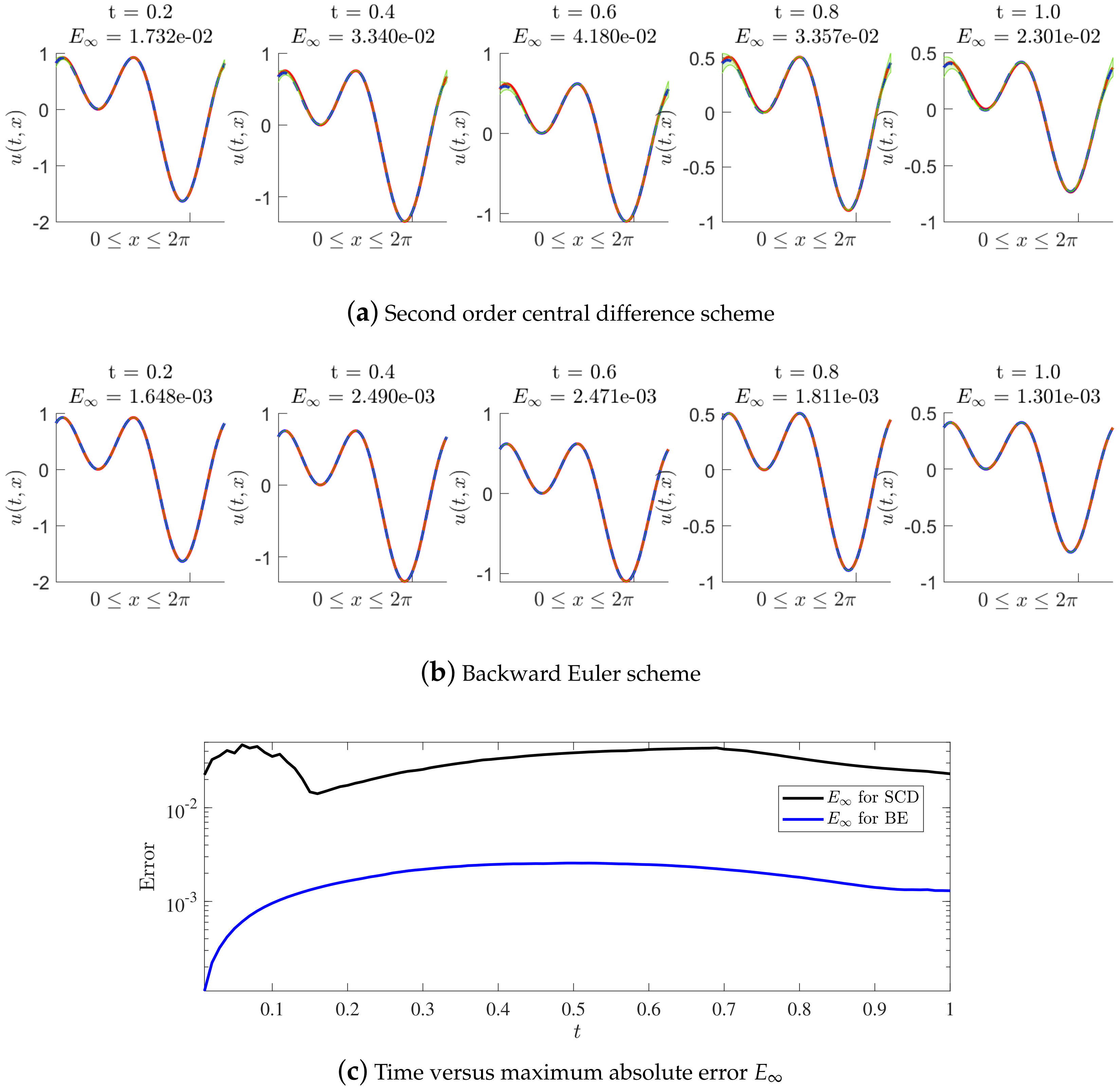
Numerical tests of solving (74) are performed with noiseless data. Figure 10 shows the posterior distribution of the predicted solution at different time nodes, where we fix the number of initial data points (inhomogeneous term data points, artificially generated data points and delay term data points) to be 15 and fix $\Delta t$ to be 0.01. Figure 9a,b, presents the results of the experiments employing the second-order central difference scheme and the backward Euler scheme, respectively, and Figure 9c shows the maximum absolute error $E_{\infty }$ with the increase in time. Moreover,

Table 8. Wave equation of Example 6: Maximum absolute error $E_{\infty }$ at some time nodes, where $\Delta t=0.01$, where the second order central difference scheme (SCD) and the backward Euler scheme (BE) are applied, respectively.

t	$0.1$	$0.2$	$0.3$	$0.4$	$0.5$
$SCD$	$3.521926\times {10}^{-2}$	$1.731871\times {10}^{-2}$	$2.562235\times {10}^{-2}$	$3.339859\times {10}^{-2}$	$3.854518\times {10}^{-2}$
$BE$	$9.577671\times {10}^{-4}$	$1.647835\times {10}^{-3}$	$2.197030\times {10}^{-3}$	$2.490295\times {10}^{-3}$	$2.566658\times {10}^{-3}$
t	$0.6$	$0.7$	$0.8$	$0.9$	$1.0$
$SCD$	$4.179861\times {10}^{-2}$	$4.218729\times {10}^{-2}$	$3.356628\times {10}^{-2}$	$2.681414\times {10}^{-2}$	$2.301241\times {10}^{-2}$
$BE$	$2.471149\times {10}^{-3}$	$2.195480\times {10}^{-3}$	$1.811016\times {10}^{-3}$	$1.411214\times {10}^{-3}$	$1.300891\times {10}^{-3}$

shows us the maximum absolute error $E_{\infty }$ at some time nodes in detail. According to the results of numerical tests, we conclude that the two methods based on MP-NGPs effectively solve the wave equation with one delay. The second method applying the backward Euler scheme behaves better than the first method, applying the second-order central difference scheme on prediction accuracy.

6. Discussion

In this paper, a new method, called multi-priors numerical Gaussian processes (MP-NGPs), is designed and proposed on the basis of numerical Gaussian processes (NGPs), to solve complex time-dependent PDEs. Compared with NGPs, the MP-NGPs proposed possess a structure with a much stricter mathematical deduction, and the application of MP-NGPs is more flexible. Delay terms and inhomogeneous terms can be introduced on MP-NGPs. The main idea of MP-NGPs is to realize the discretization of time, apply Gaussian process regression to transform the potential information of PDEs into a scheme controlled by several operators, and predict the solution from the statistical perspective. MP-NGPs build a Gaussian process regression at each time step to predict the solution at the next time step. The basic idea of MP-NGPs is very similar to that of NGPs, but the applications of MP-NGPs are explored more deeply than NGPs. Moreover, this methodology of MP-NGPs has natural advantages in handling noisy data and quantifying the uncertainty of the predicted solution. It should be mentioned that MP-NGPs can only solve a class of fractional-order PDEs composed of special fractional-order derivatives (2). Other kinds of fractional-order derivatives still deserve further research in MP-NGPs. Moreover, multi-spatial-dimension irregular domain problems, the inverse problems of PDEs, such as estimating constant or variable coefficients based on Gaussian processes and some specific application problems of MP-NGPs, may be the direction of our future investigation.

7. Conclusions

In this manuscript, the possibility of MP-NGPs in solving nonlinear delay partial differential equations with multi-delays is explored. These equations investigated include partial differential equations, partial integro-differential equations, fractional partial differential equations and wave equations. We also consider Neumann and mixed boundary conditions of PDEs on MP-NGPs. Numerical experiments prove that the method proposed can solve nonlinear delay partial differential equations with satisfactory precision, and the algorithm applying the backward Euler scheme is stably first-order accurate in time. So as to improve the prediction accuracy, Runge–Kutta methods under the frame of MP-NGPs are proposed in this manuscript. The algorithm applying the Runge–Kutta methods can effectively improve the prediction accuracy, although the temporal convergence rate of this algorithm is still of the first order according to the numerical experiments.

References

- Ghahramani, Z. Probabilistic machine learning and artificial intelligence. Nature 2015, 521, 452–459. [Google Scholar] [CrossRef] [PubMed]
- Kempa-Liehr, A.W.; Lin, C.Y.C.; Britten, R.; Armstrong, D.; Wallace, J.; Mordaunt, D.; O’Sullivan, M. Healthcare pathway discovery and probabilistic machine learning. Int. J. Med. Inform. 2020, 137, 104087. [Google Scholar] [CrossRef] [PubMed]
- Maslyaev, M.; Hvatov, A.; Kalyuzhnaya, A.V. Partial differential equations discovery with EPDE framework: Application for real and synthetic data. J. Comput. Sci. 2021, 53, 101345. [Google Scholar] [CrossRef]
- Lorin, E. From structured data to evolution linear partial differential equations. J. Comput. Phys. 2019, 393, 162–185. [Google Scholar] [CrossRef]
- Arbabi, H.; Bunder, J.E.; Samaey, G.; Roberts, A.J.; Kevrekidis, I.G. Linking machine learning with multiscale numerics: Data-driven discovery of homogenized equations. JOM 2020, 72, 4444–4457. [Google Scholar] [CrossRef]
- Martina-Perez, S.; Simpson, M.J.; Baker, R.E. Bayesian uncertainty quantification for data-driven equation learning. Proc. R. Soc. A 2021, 477, 20210426. [Google Scholar] [CrossRef] [PubMed]
- Dal Santo, N.; Deparis, S.; Pegolotti, L. Data driven approximation of parametrized PDEs by reduced basis and neural networks. J. Comput. Phys. 2020, 416, 109550. [Google Scholar] [CrossRef]
- Raissi, M.; Perdikaris, P.; Karniadakis, G.E. Physics-informed neural networks: A deep learning framework for solving forward and inverse problems involving nonlinear partial differential equations. J. Comput. Phys. 2019, 378, 686–707. [Google Scholar] [CrossRef]
- Kremsner, S.; Steinicke, A.; Szölgyenyi, M. A deep neural network algorithm for semilinear elliptic PDEs with applications in insurance mathematics. Risks 2020, 8, 136. [Google Scholar] [CrossRef]
- Guo, Y.; Cao, X.; Liu, B.; Gao, M. Solving partial differential equations using deep learning and physical constraints. Appl. Sci. 2020, 10, 5917. [Google Scholar] [CrossRef]
- Chen, Z.; Liu, Y.; Sun, H. Physics-informed learning of governing equations from scarce data. Nat. Commun. 2021, 12, 6136. [Google Scholar] [CrossRef] [PubMed]
- Gelbrecht, M.; Boers, N.; Kurths, J. Neural partial differential equations for chaotic systems. New J. Phys. 2021, 23, 043005. [Google Scholar] [CrossRef]
- Omidi, M.; Arab, B.; Rasanan, A.; Rad, J.; Parand, K. Learning nonlinear dynamics with behavior ordinary/partial/system of the differential equations: Looking through the lens of orthogonal neural networks. Eng. Comput. 2022, 38, 1635–1654. [Google Scholar] [CrossRef]
- Lagergren, J.H.; Nardini, J.T.; Michael Lavigne, G.; Rutter, E.M.; Flores, K.B. Learning partial differential equations for biological transport models from noisy spatio-temporal data. Proc. R. Soc. A 2020, 476, 20190800. [Google Scholar] [CrossRef]
- Koyamada, K.; Long, Y.; Kawamura, T.; Konishi, K. Data-driven derivation of partial differential equations using neural network model. Int. J. Model Simulat. Sci. Comput. 2021, 12, 2140001. [Google Scholar] [CrossRef]
- Kalogeris, I.; Papadopoulos, V. Diffusion maps-aided Neural Networks for the solution of parametrized PDEs. Comput. Meth. Appl. Mech. Eng. 2021, 376, 113568. [Google Scholar] [CrossRef]
- Kaipio, J.; Somersalo, E. Statistical and Computational Inverse Problems; Springer Science & Business Media: New York, NY, USA, 2006; Volume 160. [Google Scholar] [CrossRef]
- Williams, C.K.; Rasmussen, C.E. Gaussian Processes for Machine Learning; MIT Press: Cambridge, MA, USA, 2006; Volume 2. [Google Scholar] [CrossRef] [Green Version]
- Mahmoodzadeh, A.; Mohammadi, M.; Abdulhamid, S.N.; Ali, H.F.H.; Ibrahim, H.H.; Rashidi, S. Forecasting tunnel path geology using Gaussian process regression. Geomech. Eng. 2022, 28, 359–374. [Google Scholar] [CrossRef]
- Hoolohan, V.; Tomlin, A.S.; Cockerill, T. Improved near surface wind speed predictions using Gaussian process regression combined with numerical weather predictions and observed meteorological data. Renew. Energy 2018, 126, 1043–1054. [Google Scholar] [CrossRef]
- Gonzalvez, J.; Lezmi, E.; Roncalli, T.; Xu, J. Financial applications of gaussian processes and bayesian optimization. arXiv 2019, arXiv:1903.04841. [Google Scholar] [CrossRef] [Green Version]
- Schölkopf, B.; Smola, A.J.; Bach, F. Learning with Kernels: Support Vector Machines, Regularization, Optimization, and beyond; MIT Press: Cambridge, MA, USA, 2002. [Google Scholar]
- Drucker, H.; Wu, D.; Vapnik, V.N. Support vector machines for spam categorization. IEEE Trans. Neural Netw. 1999, 10, 1048–1054. [Google Scholar] [CrossRef] [PubMed] [Green Version]
- Tipping, M.E. Sparse Bayesian learning and the relevance vector machine. J. Mach. Learn. Res. 2001, 1, 211–244. [Google Scholar]
- Lange-Hegermann, M. Linearly constrained gaussian processes with boundary conditions. In Proceedings of the International Conference on Artificial Intelligence and Statistics, PMLR, San Diego, USA, 13–15 April 2021; pp. 1090–1098. [Google Scholar]
- Gahungu, P.; Lanyon, C.W.; Alvarez, M.A.; Bainomugisha, E.; Smith, M.; Wilkinson, R.D. Adjoint-aided inference of Gaussian process driven differential equations. arXiv 2022, arXiv:2202.04589. [Google Scholar] [CrossRef]
- Gulian, M.; Frankel, A.; Swiler, L. Gaussian process regression constrained by boundary value problems. Comput. Methods Appl. Mech. Eng. 2022, 388, 114117. [Google Scholar] [CrossRef]
- Yang, S.; Wong, S.W.; Kou, S. Inference of dynamic systems from noisy and sparse data via manifold-constrained Gaussian processes. Proc. Natl. Acad. Sci. USA 2021, 118, e2020397118. [Google Scholar] [CrossRef] [PubMed]
- Raissi, M.; Perdikaris, P.; Karniadakis, G.E. Numerical Gaussian processes for time-dependent and nonlinear partial differential equations. SIAM J. Sci. Comput. 2018, 40, A172–A198. [Google Scholar] [CrossRef] [Green Version]
- Oates, C.J.; Sullivan, T.J. A modern retrospective on probabilistic numerics. Stat. Comput. 2019, 29, 1335–1351. [Google Scholar] [CrossRef] [Green Version]
- Hennig, P.; Osborne, M.A.; Girolami, M. Probabilistic numerics and uncertainty in computations. Proc. R. Soc. A 2015, 471, 20150142. [Google Scholar] [CrossRef] [PubMed] [Green Version]
- Conrad, P.R.; Girolami, M.; Särkkä, S.; Stuart, A.; Zygalakis, K. Statistical analysis of differential equations: Introducing probability measures on numerical solutions. Stat. Comput. 2017, 27, 1065–1082. [Google Scholar] [CrossRef] [Green Version]
- Kersting, H.; Sullivan, T.J.; Hennig, P. Convergence rates of Gaussian ODE filters. Stat. Comput. 2020, 30, 1791–1816. [Google Scholar] [CrossRef]
- Raissi, M.; Karniadakis, G.E. Hidden physics models: Machine learning of nonlinear partial differential equations. J. Comput. Phys. 2018, 357, 125–141. [Google Scholar] [CrossRef] [Green Version]
- Raissi, M.; Perdikaris, P.; Karniadakis, G.E. Machine learning of linear differential equations using Gaussian processes. J. Comput. Phys. 2017, 348, 683–693. [Google Scholar] [CrossRef] [Green Version]
- Reddy, J.N. Introduction to the Finite Element Method; McGraw-Hill Education: Columbus, OH, USA, 2019. [Google Scholar] [CrossRef] [Green Version]
- Gottlieb, D.; Orszag, S.A. Numerical Analysis of Spectral Methods: Theory and Applications; SIAM: Philadelphia, PA, USA, 1977. [Google Scholar] [CrossRef] [Green Version]
- Strikwerda, J.C. Finite Difference Schemes and Partial Differential Equations; SIAM: Philadelphia, PA, USA, 2004; Available online: https://www.semanticscholar.org/paper/Finite-Difference-Schemes-and-Partial-Differential-Strikwerda/757830fca3a06a8a402efad2d812bea0cf561702 (accessed on 20 August 2022).
- Bernardo, J.M.; Smith, A.F. Bayesian Theory; John Wiley & Sons: Hoboken, NJ, USA, 2009; Volume 405, Available online: https://onlinelibrary.wiley.com/doi/book/10.1002/9780470316870 (accessed on 20 August 2022).
- Podlubny, I. Fractional Differential Equations: An Introduction to Fractional Derivatives, Fractional Differential Equations, to Methods of Their Solution and Some of Their Applications; Elsevier: Amsterdam, The Netherlands, 1998. [Google Scholar]
- Povstenko, Y. Linear Fractional Diffusion-Wave Equation for Scientists and Engineers; Birkhäuser: New York, NY, USA, 2015. [Google Scholar] [CrossRef]
- König, H. Eigenvalue Distribution of Compact Operators; Birkhäuser: Basel, Switzerland, 2013; Volume 16. [Google Scholar] [CrossRef]
- Berlinet, A.; Thomas-Agnan, C. Reproducing Kernel Hilbert Spaces in Probability and Statistics; Springer Science & Business Media: Berlin/Heidelberg, Germany, 2011. [Google Scholar] [CrossRef]
- Zhu, C.; Byrd, R.H.; Lu, P.; Nocedal, J. Algorithm 778: L-BFGS-B: Fortran subroutines for large-scale bound-constrained optimization. ACM Trans. Math. Softw. 1997, 23, 550–560. [Google Scholar] [CrossRef]
- Mirjalili, S.; Lewis, A. The whale optimization algorithm. Adv. Eng. Softw. 2016, 95, 51–67. [Google Scholar] [CrossRef]
- Dorigo, M.; Birattari, M.; Stutzle, T. Ant colony optimization. IEEE Comput. Intell. Mag. 2006, 1, 28–39. [Google Scholar] [CrossRef]
- Iserles, A. A First Course in the Numerical Analysis of Differential Equations; Number 44; Cambridge University Press: Cambridge, UK, 2009. [Google Scholar] [CrossRef]
- Butcher, J.C. A history of Runge-Kutta methods. Appl. Numer. Math. 1996, 20, 247–260. [Google Scholar] [CrossRef]
Figure 1.
Basic workflow of MP-NGPs.
Figure 2.
Fractional equation of Example 1: the posterior distribution of the predicted solution at different time nodes, where is fixed to be . The red solid line represents the exact solution. The blue dash line represents the posterior mean. The green shade indicates the two posterior standard deviation centered on the posterior mean. Noiseless data and noisy data are used, respectively.
Figure 3.
Fractional equation of Example 1: the posterior distribution of the predicted solution at different time nodes, where is fixed to be . Noiseless data and noisy data are used, respectively.
Figure 4.
Figure 5.
Integro-differential equation: the posterior distribution of the predicted solution at different time nodes, where . Noiseless data and noisy data are used, respectively.
Figure 6.
Problem of Example 3: Time versus the relative spatial error and maximum absolute error until the final time step is reached, where is fixed to be 0.01.
Figure 7.
Results of Example 4, (a) impact of the number of initial data points (inhomogeneous term data points, artificially generated data points and delay term data points) on , when the backward Euler scheme is employed. Fix to be , and in turn. (b) Impact of the level of the additive noise on the maximum absolute error , when the backward Euler scheme is used. Fix the number of initial data points (inhomogeneous term data points, artificially generated data points and delay term data points) to be 20, and take .
Figure 8.
Problem of Example 1: (a) The posterior distribution of the predicted solution at different time nodes, where the backward Euler scheme is used. Fix the number of initial data points (inhomogeneous term data points, artificially generated data points and delay term data points) to be 30, and take . (b) The posterior distribution of the predicted solution at different time nodes, where the trapezoidal scheme is used. The other experimental conditions are the same as those with the backward Euler scheme. (c) Time versus maximum absolute error until the final time step is reached, where the backward Euler scheme and the trapezoidal scheme are both considered.
Figure 9.
(a) The posterior distribution of the predicted solution at different time nodes, where Dirichlet boundary conditions are employed. (b) The posterior distribution of the predicted solution at different time nodes, where Neumann boundary conditions are employed. (c) The posterior distribution of the predicted solution at different time nodes, where mixed boundary conditions are employed. (d) Time versus the maximum absolute error until the final time step is reached.
Figure 10.
Wave equation of Example 6: (a) The posterior distribution of the predicted solution at different time nodes, where the second order central difference scheme is used. (b) The posterior distribution of the predicted solution at different time nodes, where the backward Euler scheme is used. (c) Time versus maximum absolute error until the final time step is reached, where the second order central difference scheme (SCD) and the backward Euler scheme (BE) are both considered.