
Spatial Series and Fractal Analysis Associated with Fracture Behaviour of UO2 Ceramic Material

1
School of Engineering, Swiss Federal Institute of Technology (EPFL), 1015 Lausanne, Switzerland
2
Division Radio Monitoring and Equipment, Section Market Access and Conformity, Federal Office of Communications OFCOM, 2501 Bienne, Switzerland
3
Five Rescue Research Laboratory, 75004 Paris, France
4
Department of Physics, Faculty of Applied Sciences, University Politehnica of Bucharest, 060042 Bucharest, Romania
5
Academy of Romanian Scientists, 050094 Bucharest, Romania
*
Author to whom correspondence should be addressed.
Fractal Fract. 2022, 6(10), 595; https://doi.org/10.3390/fractalfract6100595
Submission received: 17 August 2022
/
Revised: 18 September 2022
/
Accepted: 10 October 2022
/
Published: 14 October 2022
(This article belongs to the Special Issue Nonlinear Dynamics in Complex Systems via Fractals and Fractional Calculus)
Abstract
:SEM micrographs of the fracture surface for UO2 ceramic materials have been analysed. In this paper, we introduce some algorithms and develop a computer application based on the time-series method. Utilizing the embedding technique of phase space, the attractor is reconstructed. The fractal dimension, lacunarity, and autocorrelation dimension average value have been calculated.
1. Introduction
The uranium chemical element has the capital letter U as its symbol, and its atomic number is 92. Statistically speaking, it constitutes three important isotopes that may definitely be found in nature: 238U (99.28% abundance), 235U (0.71% abundance), and 234U (0.0054% abundance). Classified in the periodic table as an actinide, uranium is generally a solid body at room temperature [1]. Uranium is a naturally radioactive element, from the physics viewpoint. It powers nuclear reactors in the form of nuclear fuel and helps to make atomic bombs (still improperly called), but more precisely, named nuclear bombs, because fission is a nuclear process.
Uranium-235 is an isotope of uranium that makes up about 0.71% of naturally existing uranium in nature. Unlike the predominant isotope uranium-238 (fertile material), uranium-235 is a fissile material; that is, they can support a nuclear chain reaction and a nuclear fission, respectively. Moreover, uranium-235 is the only fissile isotope that exists in nature as a primordial nuclide.
At first sight, real ceramic materials may be interpreted as inorganic and non-metallic materials. They are typically crystalline in nature (but may also contain a combination of glassy and crystalline phases) and are compounds formed among metallic and non-metallic elements. Chemically speaking, they are materials with atomic and ionic bonds, of which the complex hyaline structure is obtained by sintering. This is basically responsible for many of the properties of ceramics [2,3,4]. The word ceramic comes from the Greek word keramicos, which in direct translation, means burnt clay. In conclusion, being typically a crystalline construction, it can be considered traditionally as a mixed compound mostly made of metallic and non-metallic elements, so a composite material.
Ceramic materials are usually fabricated by the application of heat (at high temperatures) upon processed clays and other natural crude materials (especially in powder form) to shape a rigid solid product. Ceramic final products that reasonably utilize rocks and minerals as a starting point must endure certain processing in order to command the particle size; potion purity; particle size repartition; and finally, the heterogeneity of the mixture. These important characteristics play a major role in the total properties of the completed ceramics. From a chemical point of view, ceramic materials are mainly metallic and non-metallic oxides. In conclusion, the clays from which they are obtained are part of the large category of alumino-silicates, substances present in a high percentage in the Earth’s crust [2]. Combustion results in a crystalline internal structure, with covalent and electrovalent (ionic) chemical bonds between the constituent atoms and molecules, but we do not wish to go into such details here.
Worth knowing is also the fact that, when uranium dioxide (UO2), recognized as nuclear fuel, is stuffed with supplementary ions of oxygen in the meshes of the network, it can form nonstoichiometric compounds (e.g., UO2+x,), of which the composition may change with the function of exterior environmental conditions, among which we enumerate temperature itself and the partial pressure of oxygen. The fracture comportment of a sintered ceramic UO2 substance has been studied in light of microstructural (micro porosity, grain size, etc.) parameters, with everything being in the function of the most adequate composition delivered and the final architecture. Utilizing SEM images as an investigation method, the fracture properties have been evaluated and compared for different microstructural conditions present in the same sample of solid ceramic materials and in a sintered UO2 pellet specimen. As a general conclusion, we can consider that the fracture strength in the low-density area was superior in contrast to the that of the high-density area. Among other things, this was assigned to fissure-type deflection and bifurcation at the grain boundary, expected as owed to the porosity presence. This paper realizes an investigation of the uranium dioxide SEM pictures by utilizing the time series evaluation procedures and fractal analysis, a natural prolongation of a usual research executed before but on ductile materials [5,6,7,8].
Being justified by recent developments in inferential statistical analysis procedures for chaotic modular processes and by the new concept of spatial chaos, we introduce a continuation of deterministic boarding of the structural microscopic study of ceramic integral materials.
The work in this paper is highlighted in four sections. The first section introduces the background of the use of uranium dioxide (UO2) as nuclear fuel and ceramic materials in general. The second section focuses on providing theoretical support regarding the fractal dimension, lacunarity, and time (spatial) series. The third section introduces the results obtained and elaborates on them in a discussion. Finally, the paper concludes in the fourth and last section devoted to the conclusions.
2. Theoretical Background in Brief
2.1. Fractal Dimension and Lacunarity
The fractal-image-specific feature highlighted here is the fractal dimension, conditioned by the following formula:
where N is the cell number and ε is the cell size [9,10].
The lacunarity numerical value is computed in accordance with the following formula:
when σ is the standard deviation of the mass and μ is also the mass average value out of the total picture [11,12]. To estimate the fractal dimension, it is necessary to compose a graphic and afresh; to calculate the lacunarity, the graphical algorithm of least squares must be utilized [13,14].
2.2. Time (Spatial) Series
Let T be a dynamic system in the classical sense. More precisely, T is said to be such a mathematical object (in fact a system) if there exists a map f: X → X, such that
Let F: X→ R be a map with real determinations, which can be considered a mathematical measure of physical state space in Lagrange sense. If the variables can be appreciated as being fixed (τ is named time delay) and is a stationary state, then a repeated measurement succession
can be named as a time series (beginning with (t, x)) correlated to T [15,16].
For the determined state , a correlated time (spatial) series with the discrete dynamical system (see definition above) is written as
By definition, we call being an attractor (or attraction group) for the system T a mathematical object that has the following qualities:
- (1)
- is a nonempty set;
- (2)
- K is closed;
- (3)
- K is invariant, i.e., , for all .
Moreover, it is stated that there is a vicinity such that
Takens Embedding Theorem [17] is the principal outcome that theoretically permits attractor reconstruction for a physical dynamical system, which begins from the numerical data of one algebraic time series. Thus, if K is a dense invariant set of T and if b is the box-counting fractal dimension of K, then the map
is described by
The function defined above is generically injective. Analytically speaking, a property is called generic if the mentioned quality on a set that comprises a countable intersection of open dense sets is true [18,19]. A spatial series is, by definition, a suite of observations made on an orderly variable with regard to two structural coordinates. However, in such data, usually, the necessary statistical independence is absent. Regarding spatial series in statistics, we must think about random spatial series and how such a data series works mathematically. A spatial series, but mostly a random spatial series, is an assembly of casual variables F(x1, x2, …, xn), called random variables, a set of functions depending on certain spatial coordinates (x1, x2, …, xn).
We try to construct a statistical series of the second order, in other words, a series for which (x1, x2, …, xn) argument fluctuates only on an ordinary Cartesian grid/lattice. Utilizing the appropriations of the linear (Hilbert) space connected to the series of data, the notions of novelty and a complete nondeterministic series are highlighted [15].
Regarding the comportment of a time (spatial) series (in other words, the quality of randomness), this one can be investigated by calculating the autocorrelation function value, which is an estimate of the influence of past states on the future state [16,17]. As far as that goes, a discrete dynamical system T interpreted by the map f: X→X, the autocorrelation function formula associated with the spatial series is determined as follows:
where m is the time-average function:
2.3. SEM Picture Exploration
Chaotic statistical comportment has been proven in numerous physical, chemical, economic, and biological natural processes. Today, just two statistical chaos physics concepts are unanimously accepted. The primal conception is the temporal chaos for which any function of variables in phase space are time-dependent. The second conception, the spatial statistical chaos concept, indicates a chaos state of these data with respect to spatial coordinates. This philosophical vision opens the way for accession to nonlinear deterministic procedures/technics of spatiotemporal phenomena [16].
Even though fundamental elements of ceramic thermo-mechanical comportment are recognized, the nature, interplay, and multitude of physical, chemical, and ambient variables implicated in the engendering of a true microstructure cannot be exactly defined. Therefore, it seems legitimate to adopt a viable viewpoint and to consider the micro fractures as various textures, in fact veritable ‘black boxes’, which have been caused by two independent processes, respectively, a stochastic process (in a large sense) or another process related to matter manifestation in the format of deterministic spatial chaos [20]. As a primary check, if the studied sample could be an expression of deterministic chaos, we can be mastering methods of classical time series analysis found at disposition, which refer to an estimation of the power spectrum and autocorrelation function, in principle. To come into possession of particular characteristics of the system, it is necessary for the attractor reconstruction techniques to be applied, which allows for estimations of the Lyapunov exponent and of the correlation dimension.
For the study of UO2 SEM pictures, we used computer programming initially created for metallic or alloy materials but subsequently excellently adapted to ceramic materials, a software application that generates a time series associated with the image, then reconstructs the associated attractor, and finally computes its autocorrelation dimension [21]. The procedure for investigating a SEM picture (micrograph) is debuted by loading an image bitmap version in the computer software application used. The first step in our consideration is to generate the weighted fractal dimensions map (WFDM) through which the potential modified structures themselves are revealed (conformable to a precedent article [15]). The second step to follow is to produce a real spatial series for a picture-selected zone, as follows: the initial picture is cut into slices that are approximatively 12–16 pixels deep; by placing all these fragments/pieces together, we procure an entire tape/strip. The spatial series s(t) is acquired by calculating the mean value of the grey level for every pixel column within the tape. The investigation of these nonlinear data suites starts with the attractor reconstruction by embedding the spatial series in an upper dimensional phase space. We establish a reasonable time delay from the beginning and then, continuing, for a determined embedding dimension d, we take into account the collection/set
which is assimilated to a formal point in a pseudo phase space and immediately constructed (the series sampling procedure).
In the end, we obtain the attractor by connecting these points that are conformable to their succession. The attractor integral correlation C(r), as a distance function, is the expectation that any two points from a phase space is separated by a Euclidian interval/distance less than or equal to r. It can now be assumed that C(r) is a power-type function of r, of which the exponent designated by D is mostly assimilated with the autocorrelation dimension. The value of D is close to the regression line slope related to autocorrelation function C(r). This method of calculation is reiterated for different embedding dimension values. We close this routine action with the autocorrelation dimension plot; with a function of the embedding dimension value; and finally, by calculating its regression line slope [22,23,24,25,26,27].
3. Results and Discussion
Further on, we offer an example of the procedure to investigate the SEM pictures of a UO2 ceramic material [23]. We emphasise/mention that the sorting of the micrographs with the referenced areas was executed as stated by the WFDM method [15]. Conforming to the mentioned procedure, three sets of characteristic images are studied as much as possible [25,26].
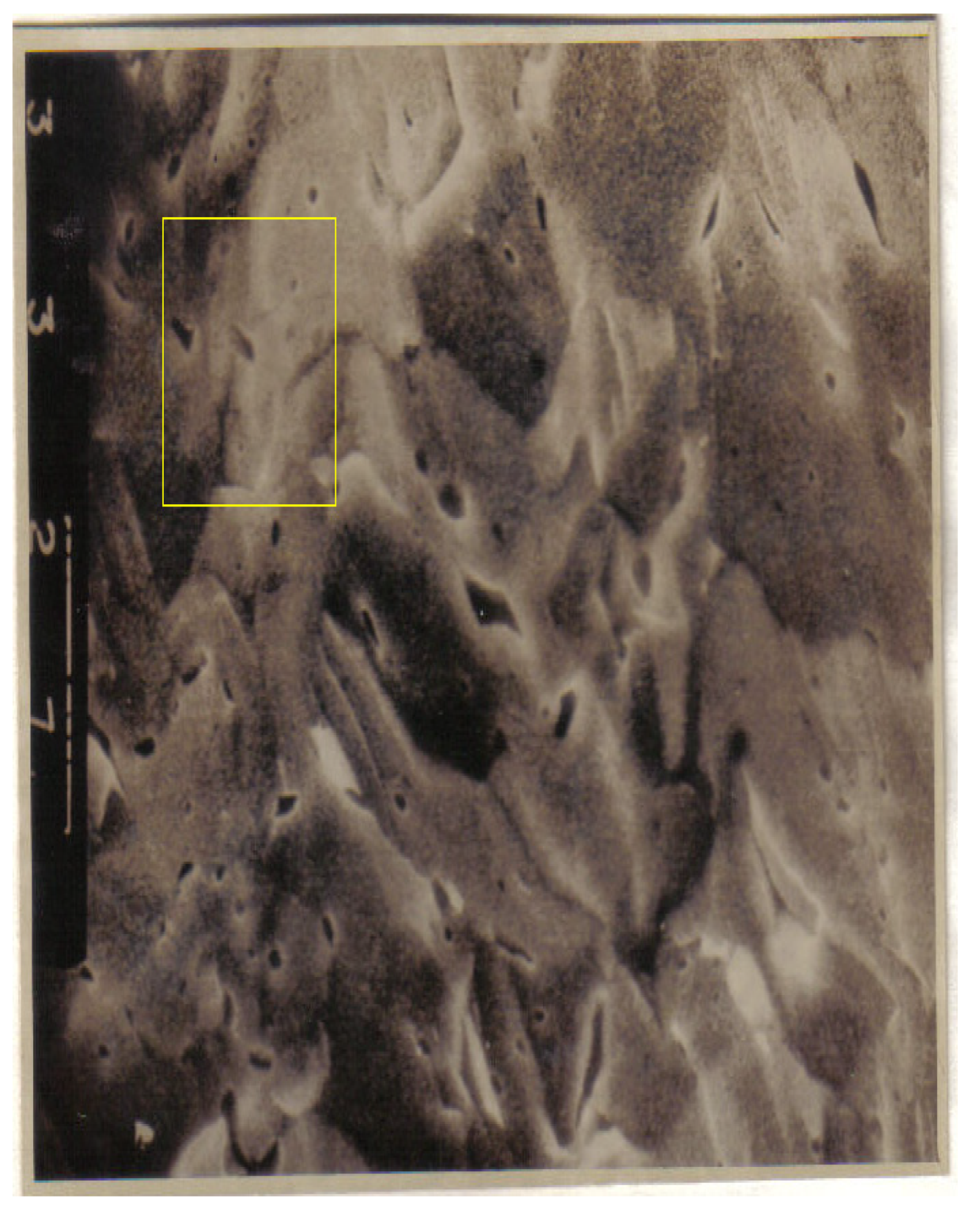
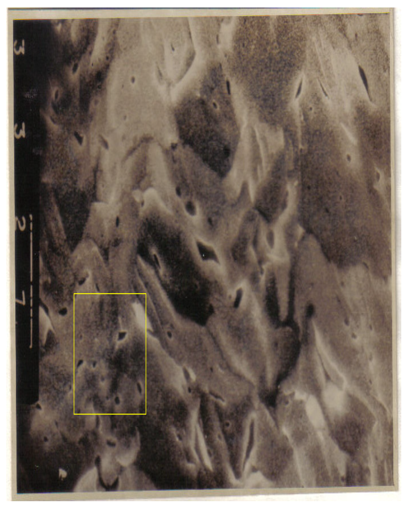
Step 1. Study of the entire picture.
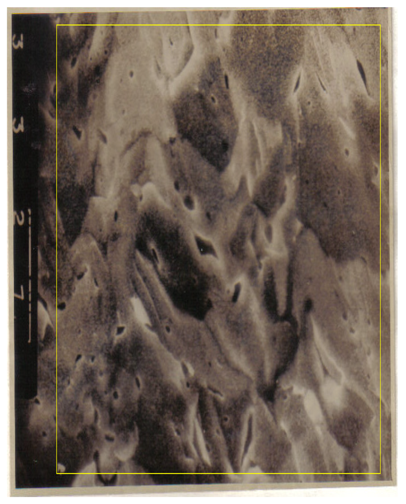
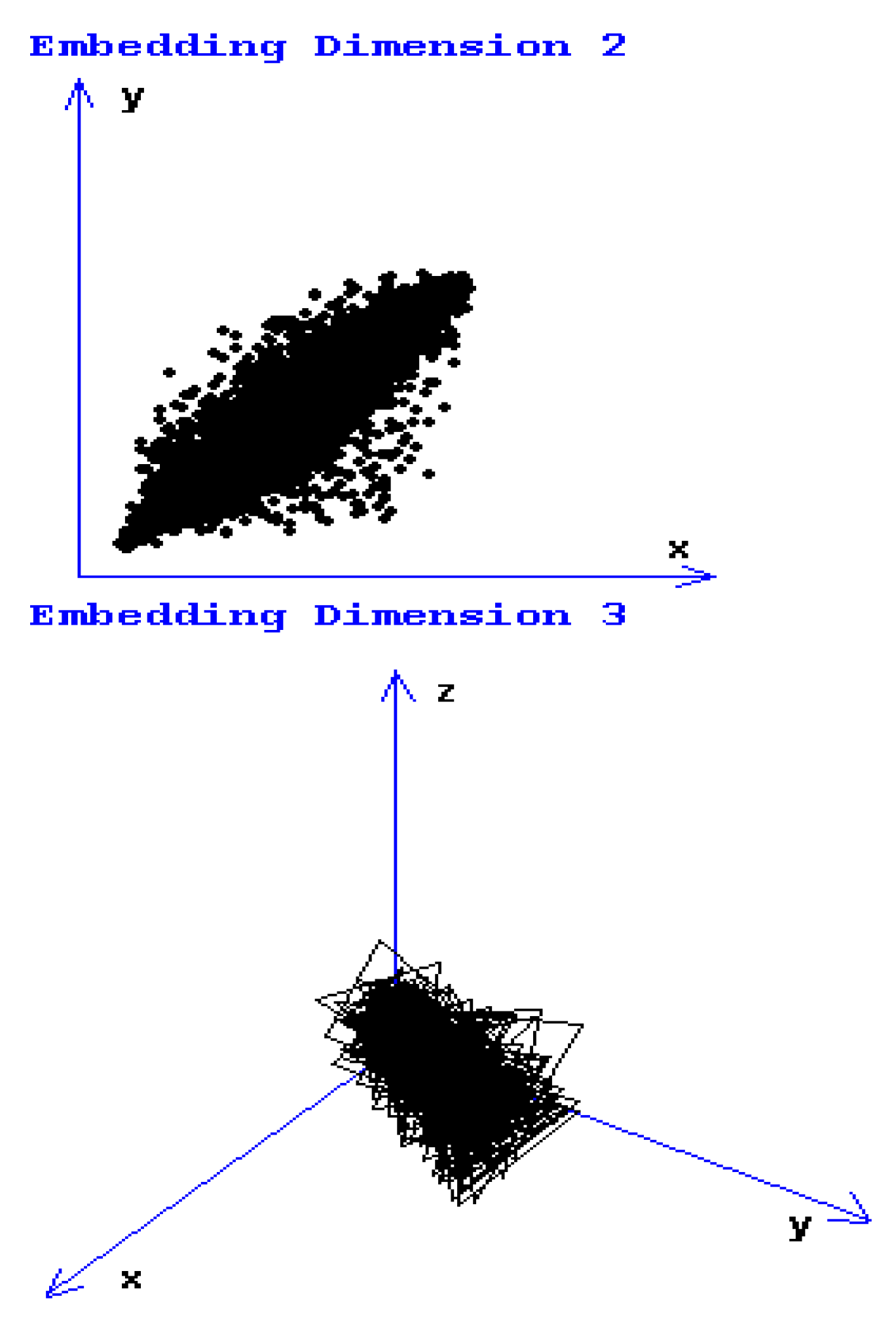
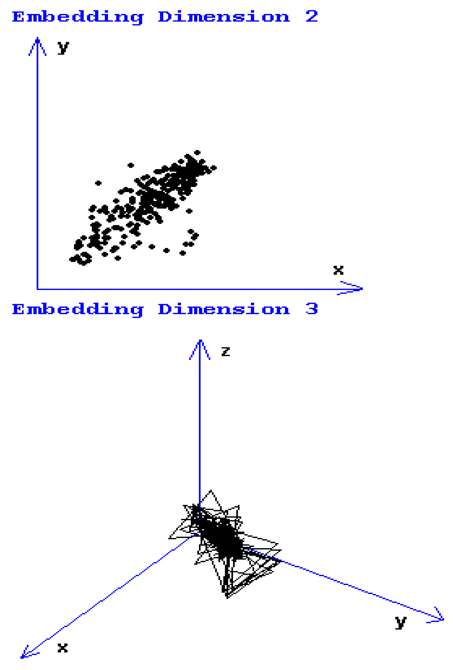
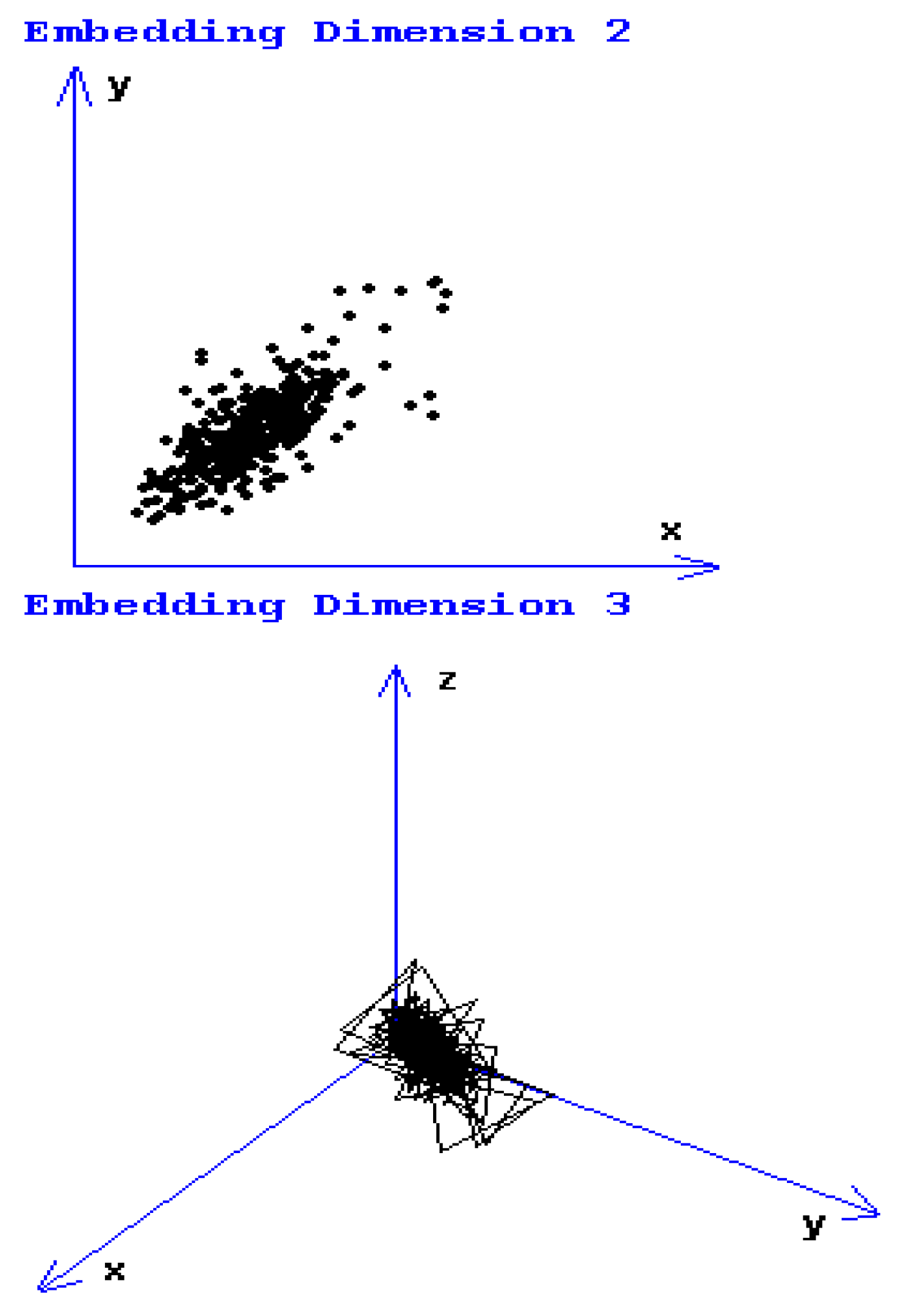
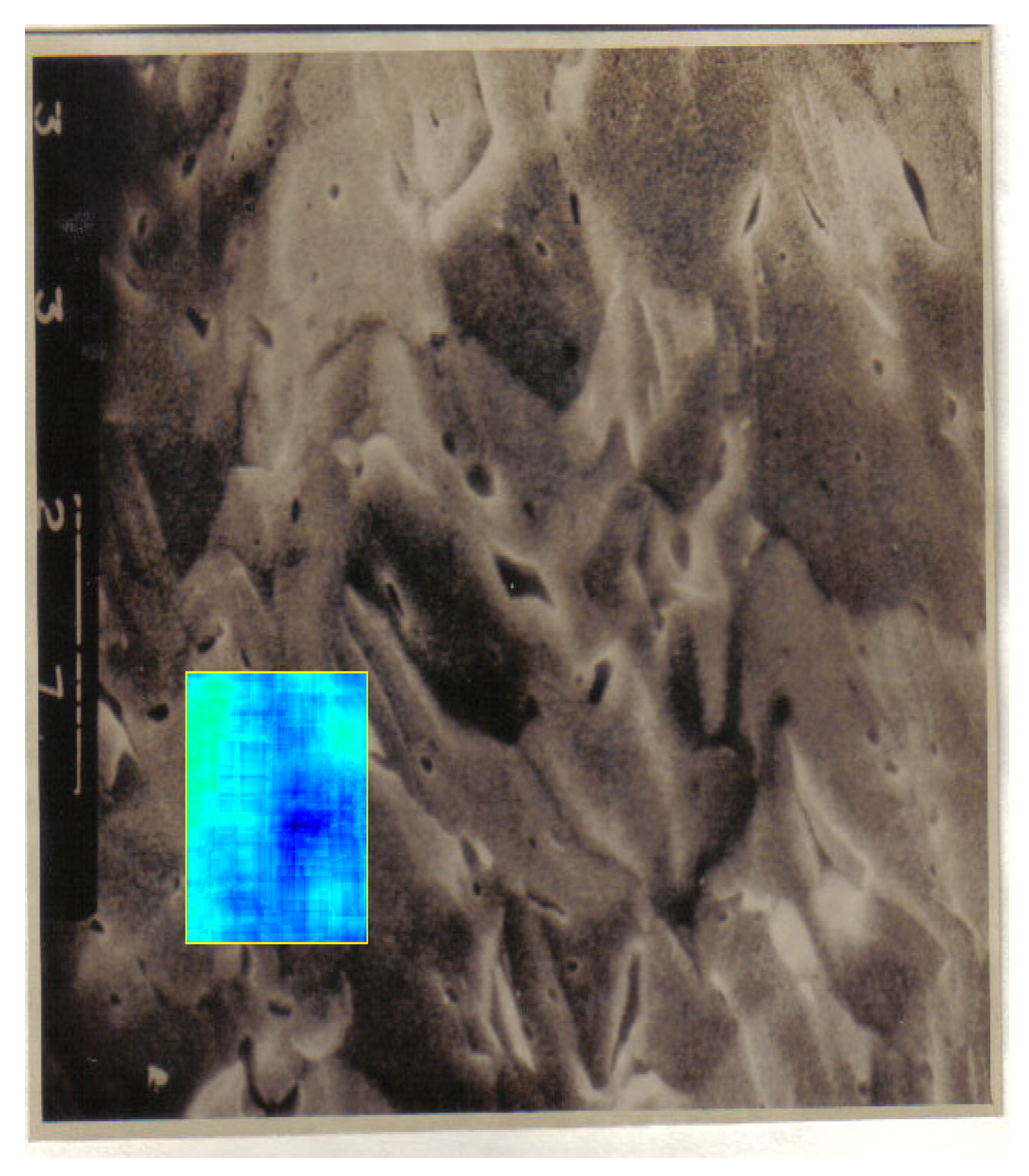
We study the images enclosed in a yellow rectangle, practically the entire picture. In Figure 1, the original SEM image and an entire selected area are presented, while in Figure 2, the graphical attractor reconstruction, in two and three dimensions, is shown.
Figure 2 shows the attractor reconstruction [20] for the rectangle with yellow sides of normal area along with a considerable area with microcracks and prominent breakage, conformable to Figure 1. Both attractor reconstructions are presented. In embedding dimension 2, some points are observed, and in embedding dimension 3, some broken lines are noticed [16,17].
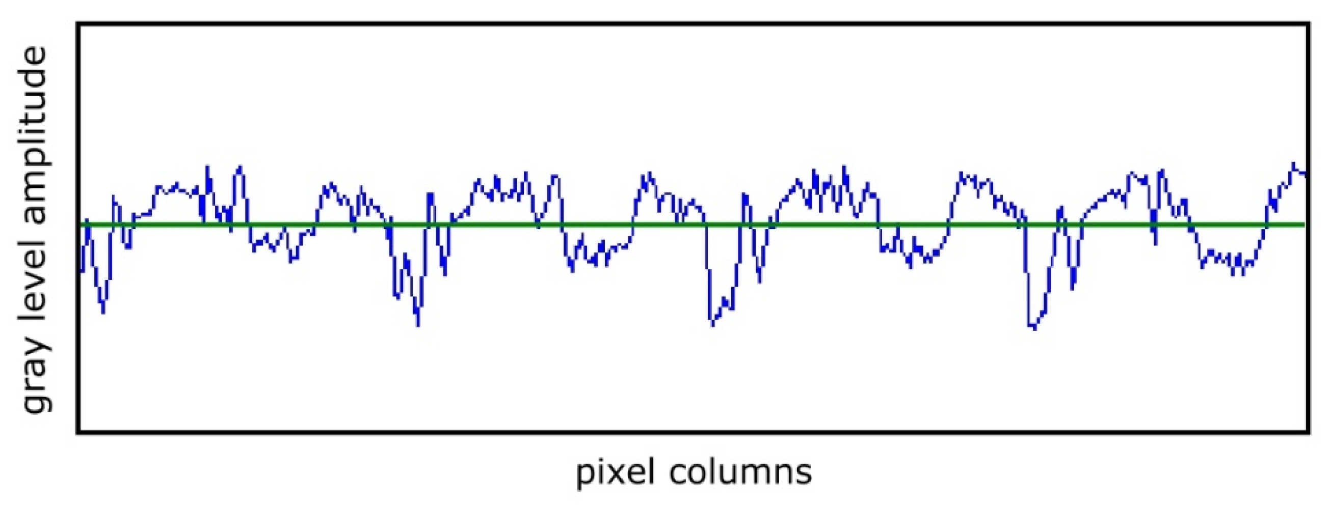
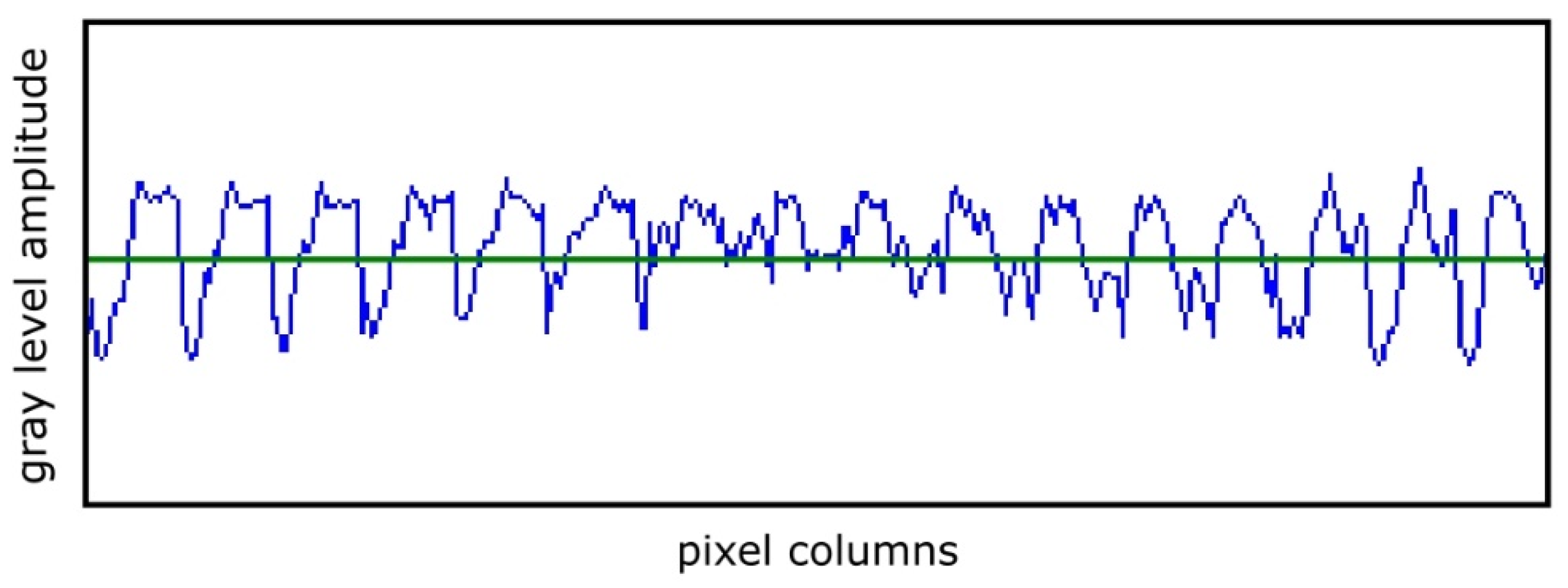
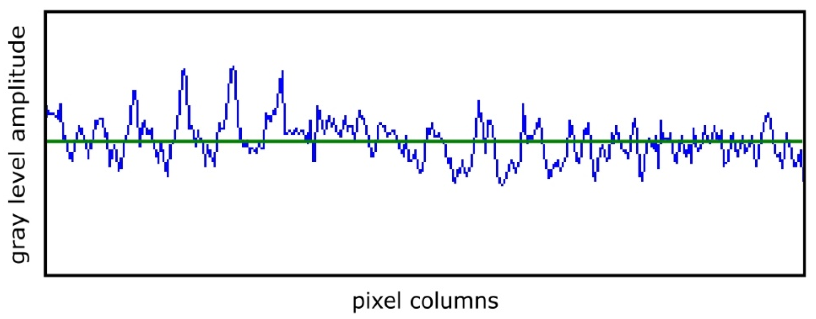
First, we survey the spatial series generated by the entire picture (Figure 3).
In Figure 3, the continuous green line placed horizontally represents the series average value over the entire time considered.
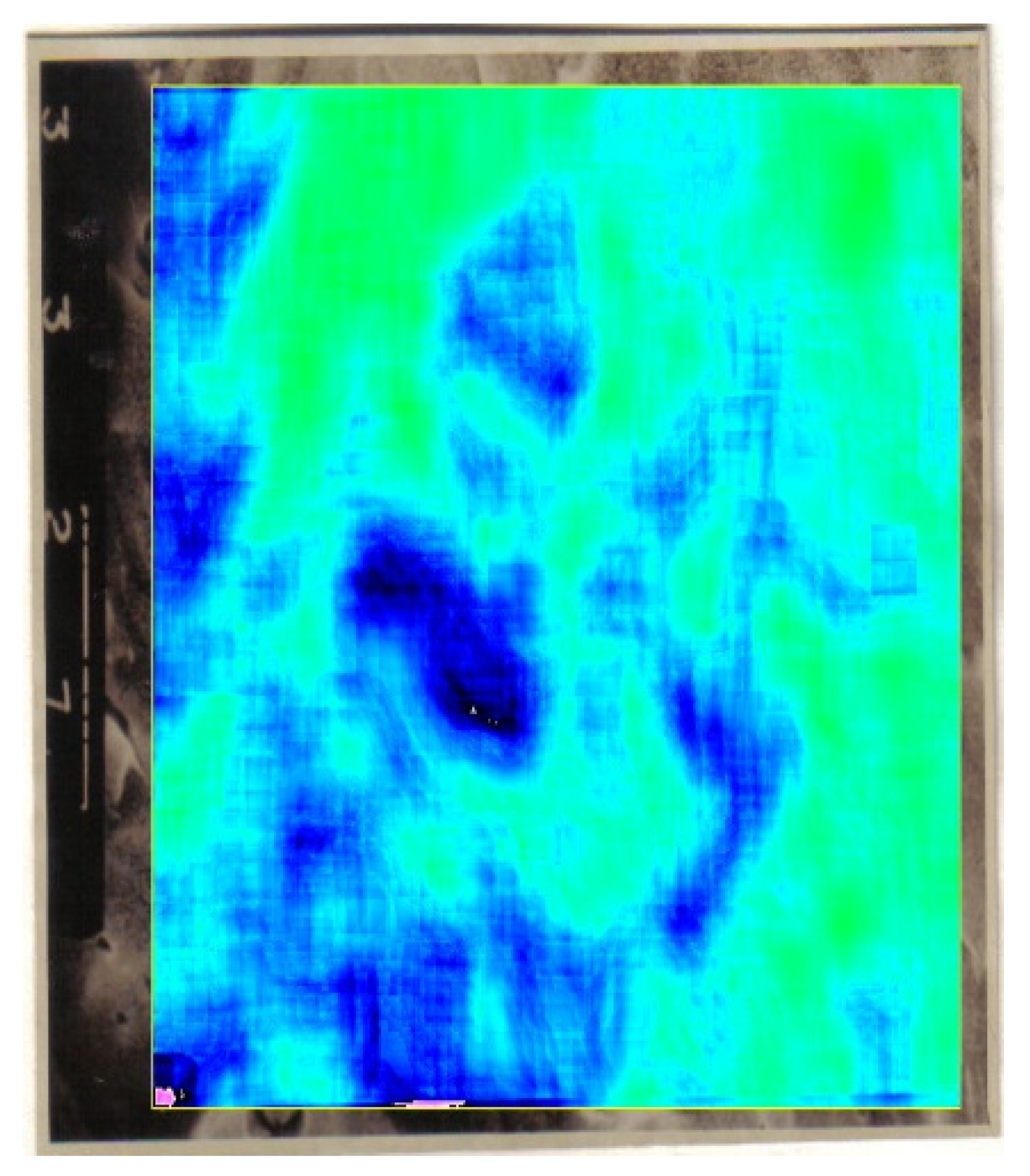
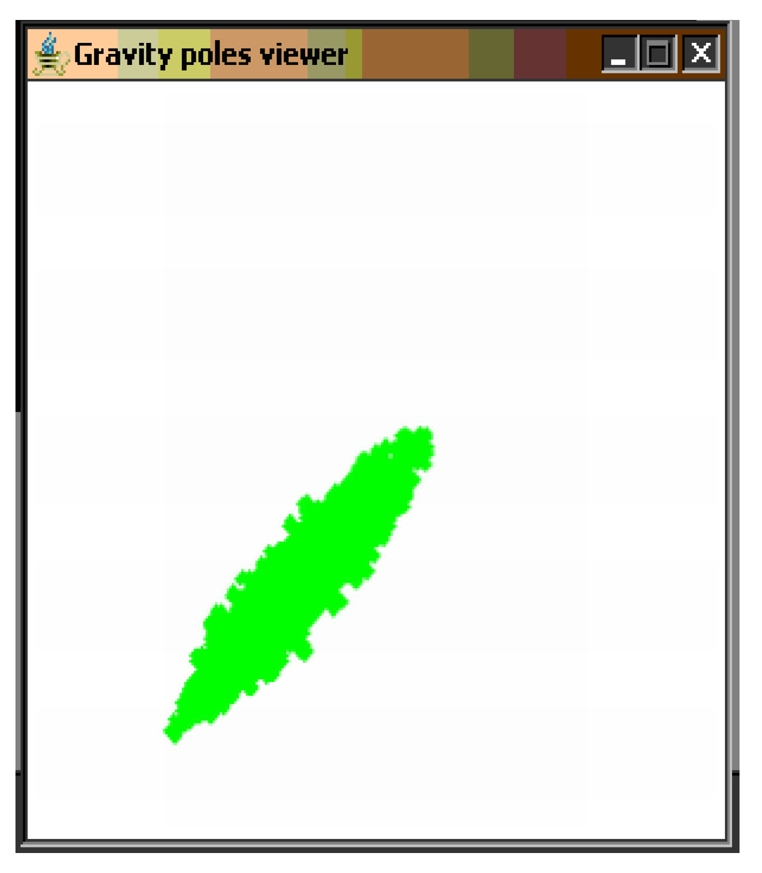
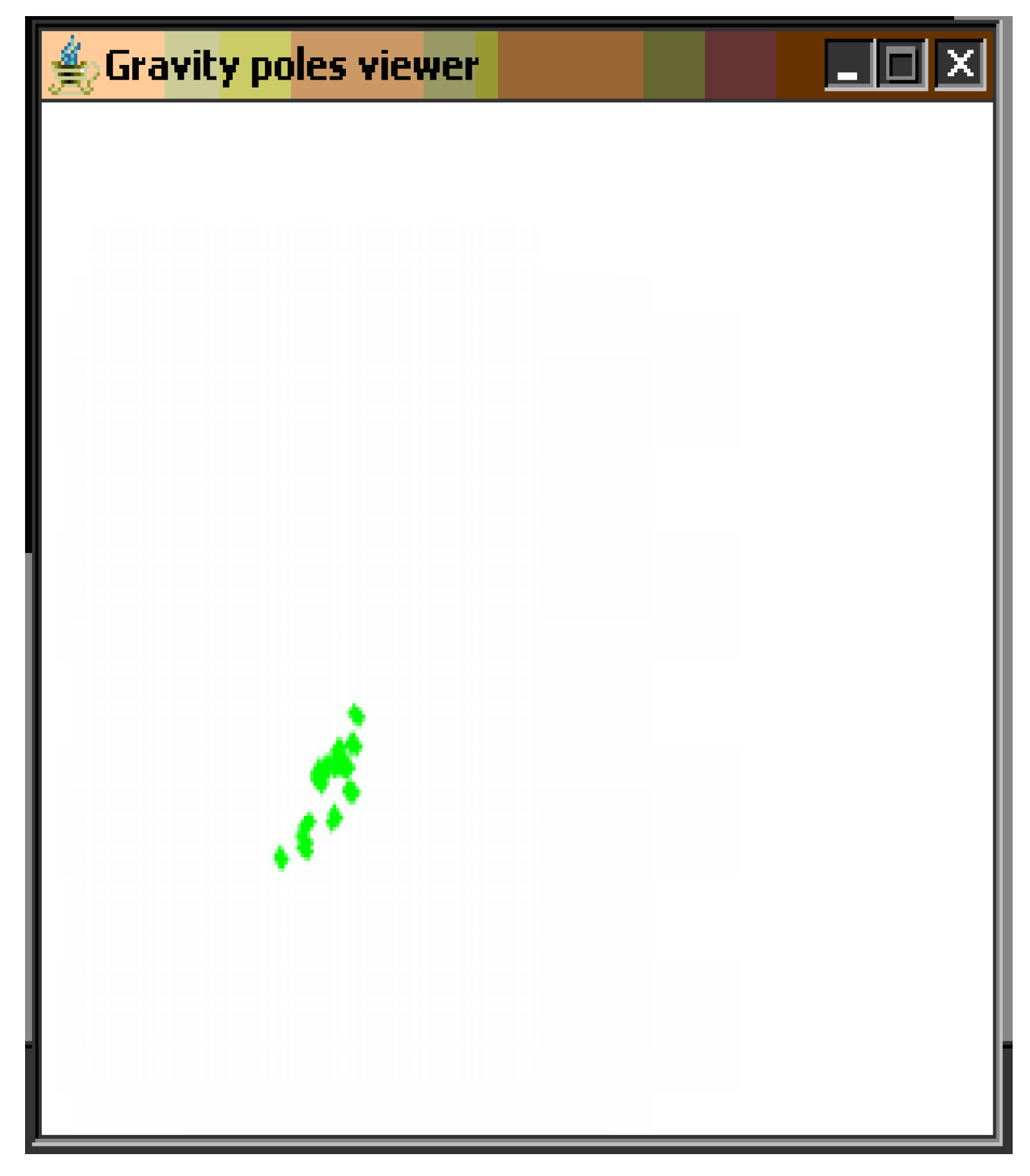
According to the algorithm, further on, we will study a modified area (Figure 4) and gravity poles are determined (Figure 5).
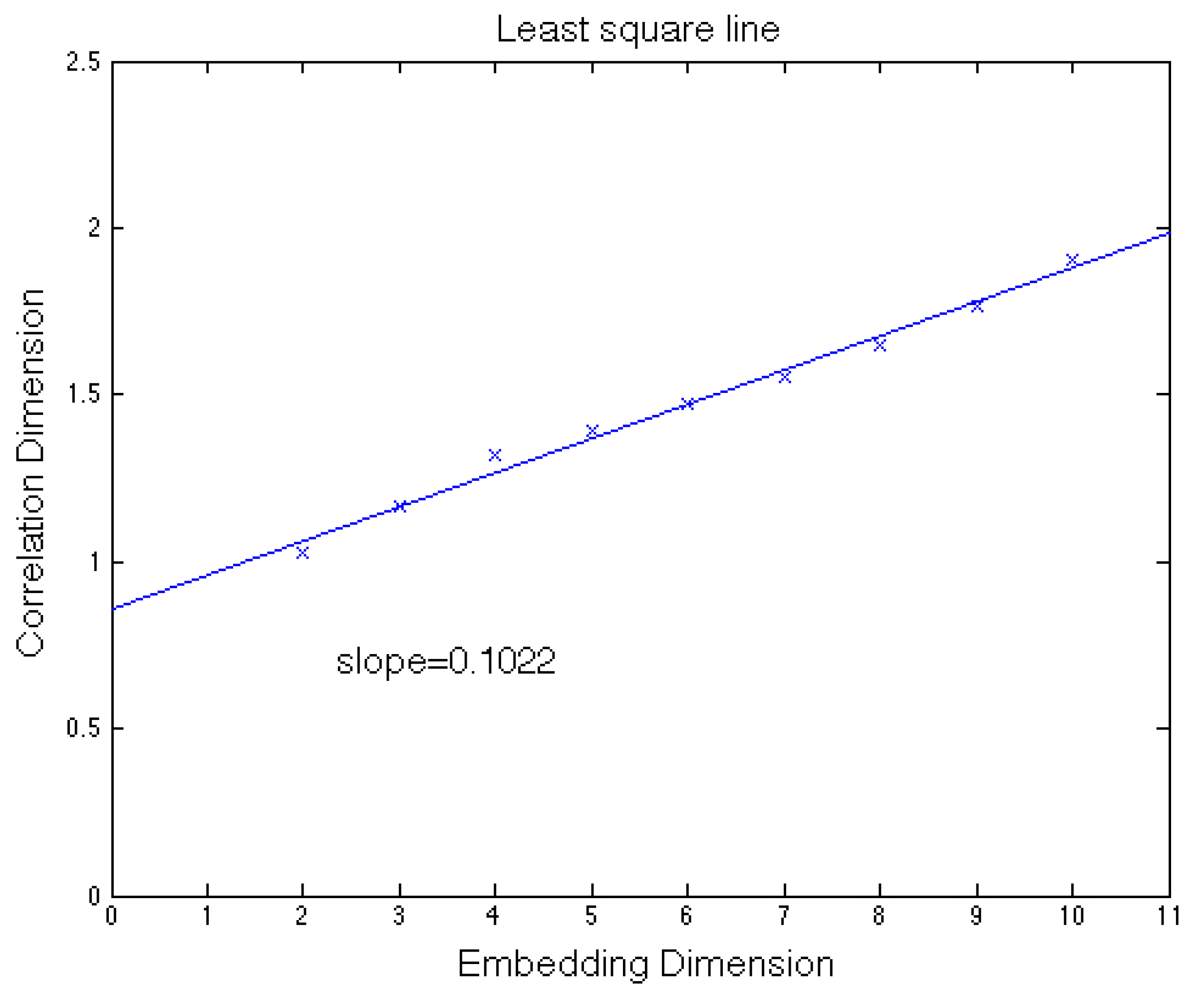
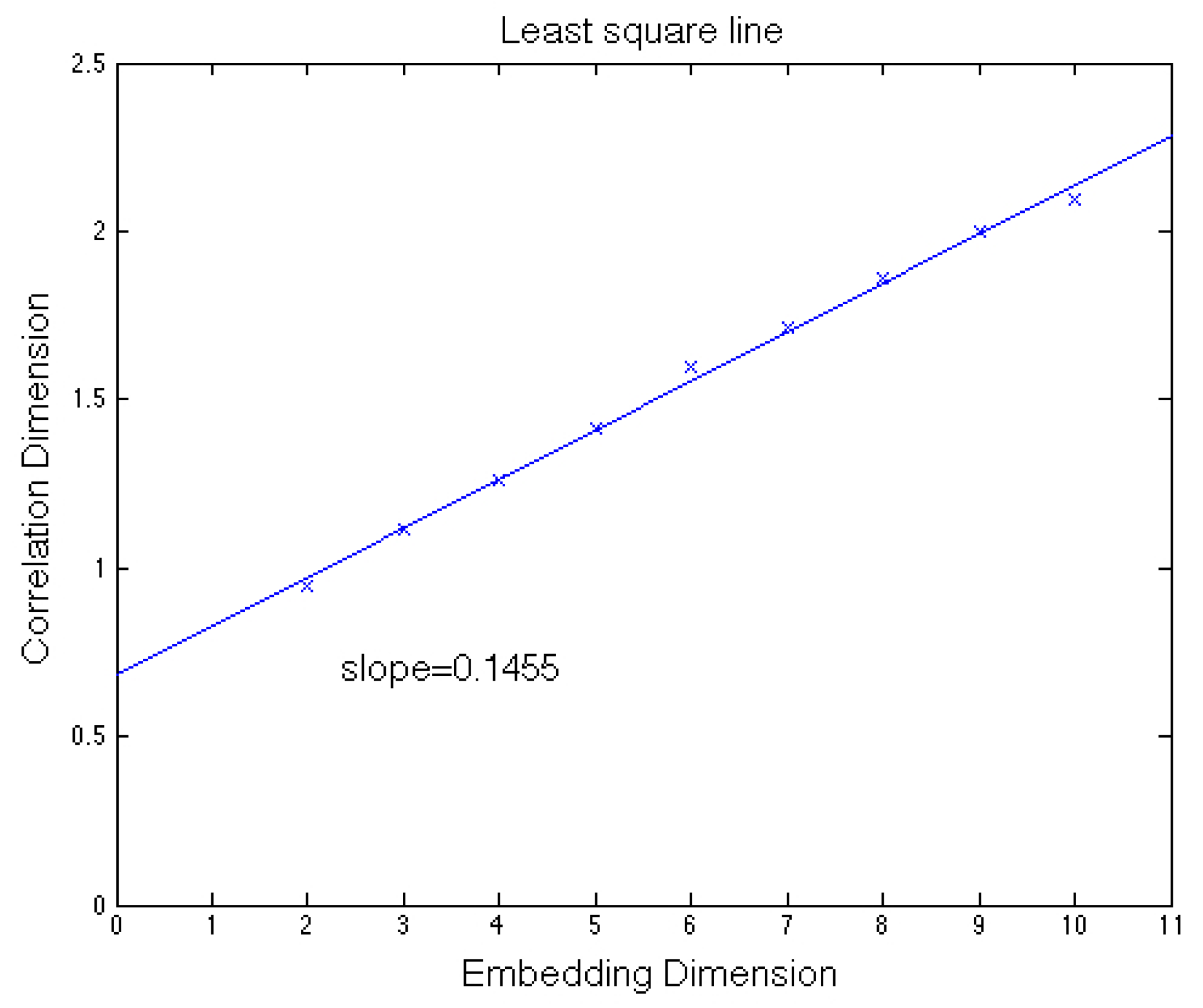
From Figure 6, we can determine the slope of the autocorrelation dimension versus the embedding dimension for the modified area.
The graphic of the entire area autocorrelation, in Figure 6, representing the correlation dimension versus the embedding dimension, shows the slope computation. The correlation dimension versus the embedding dimension slope is 0.1022.
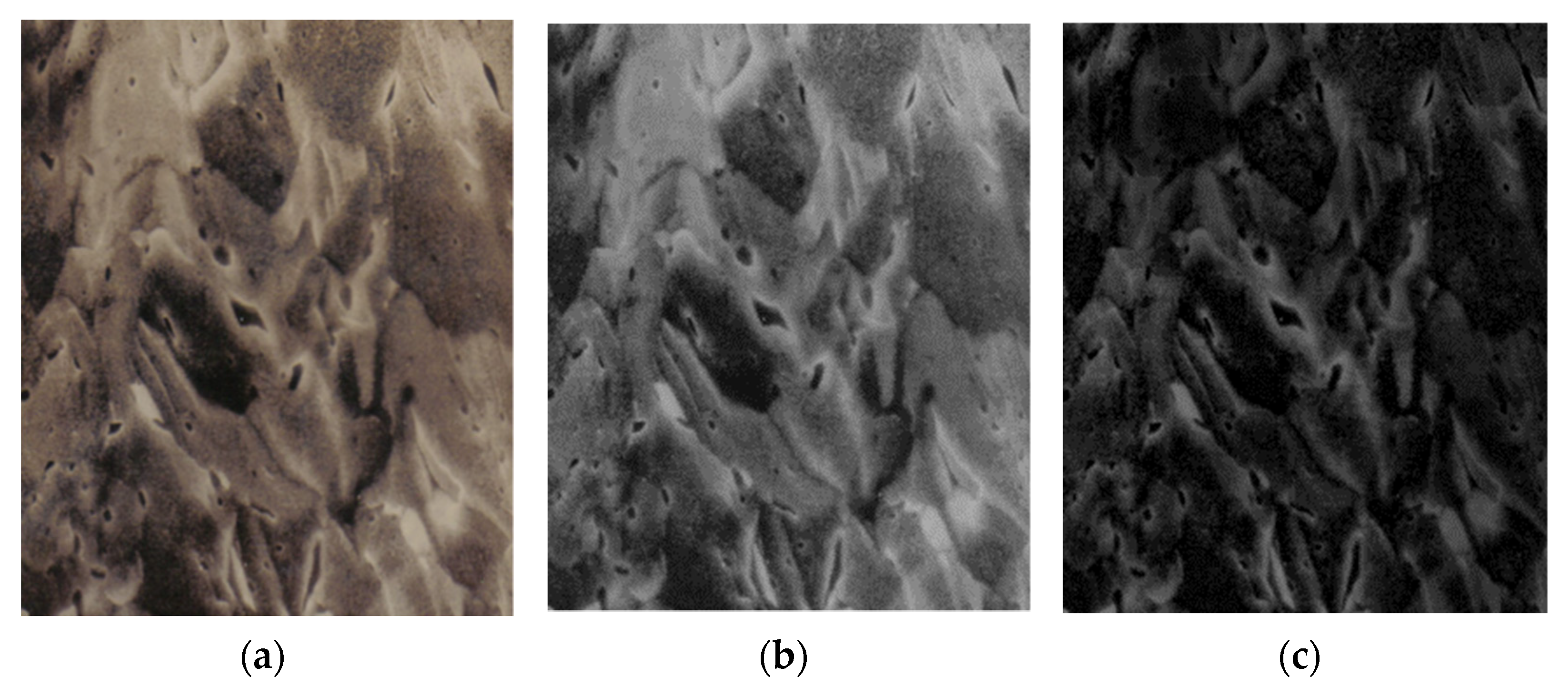
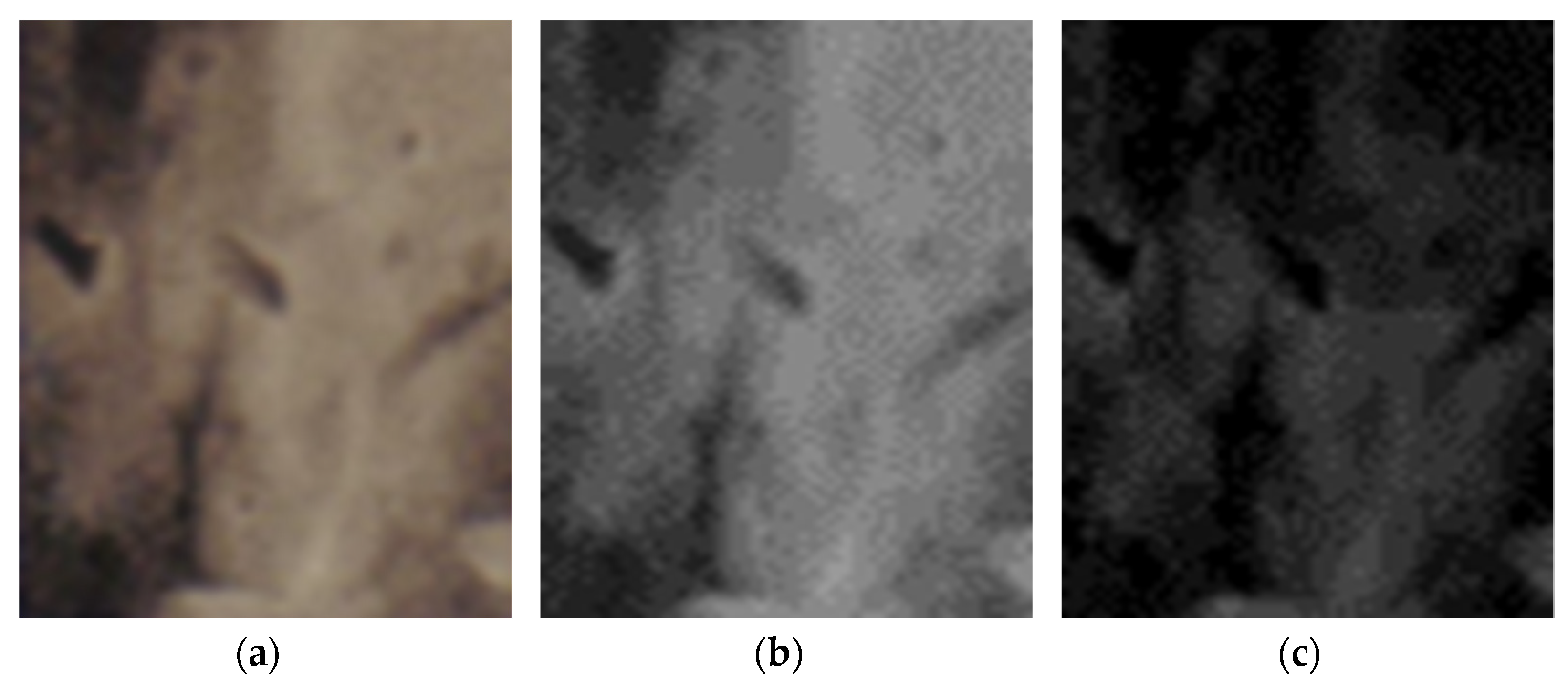
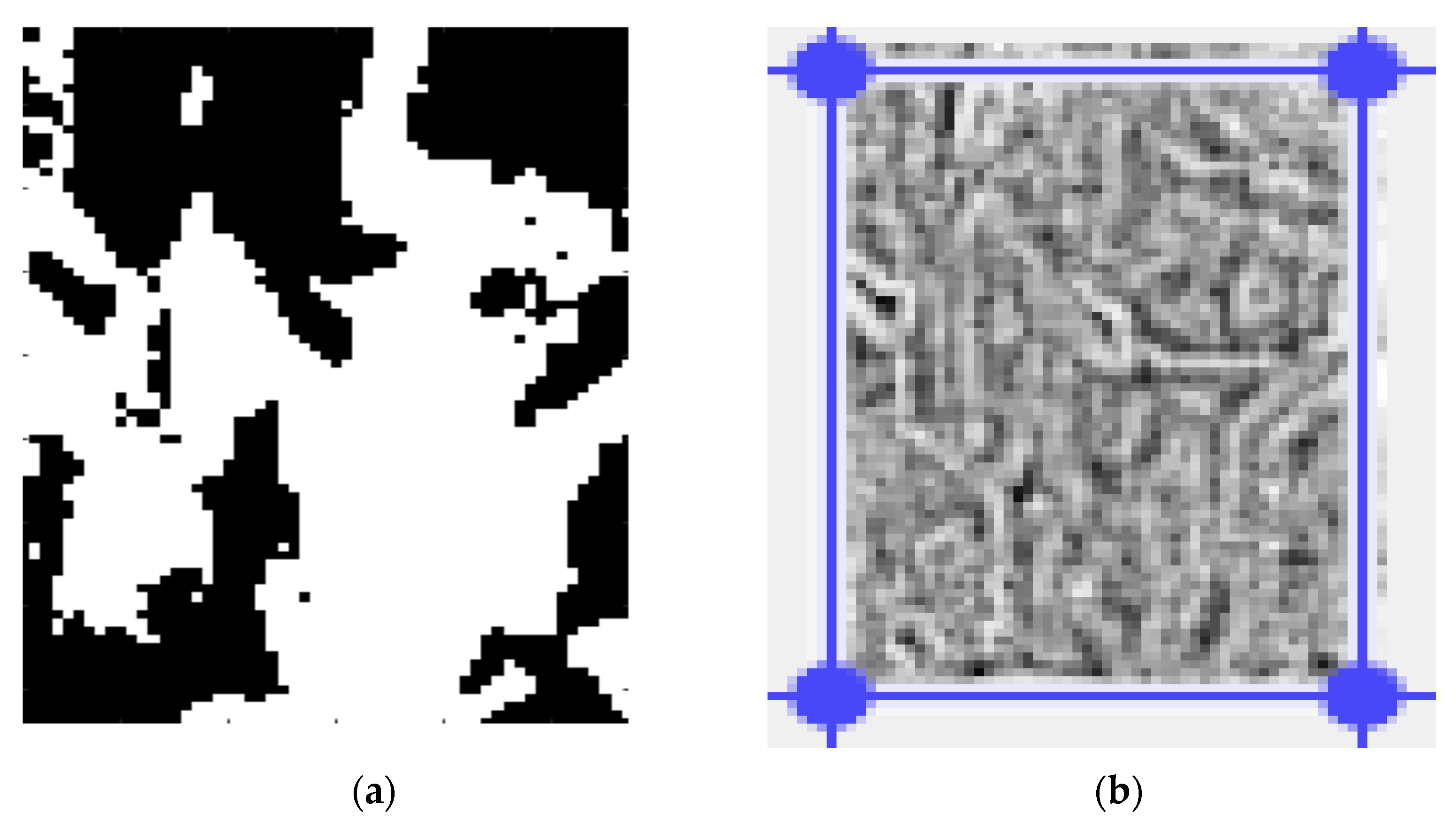
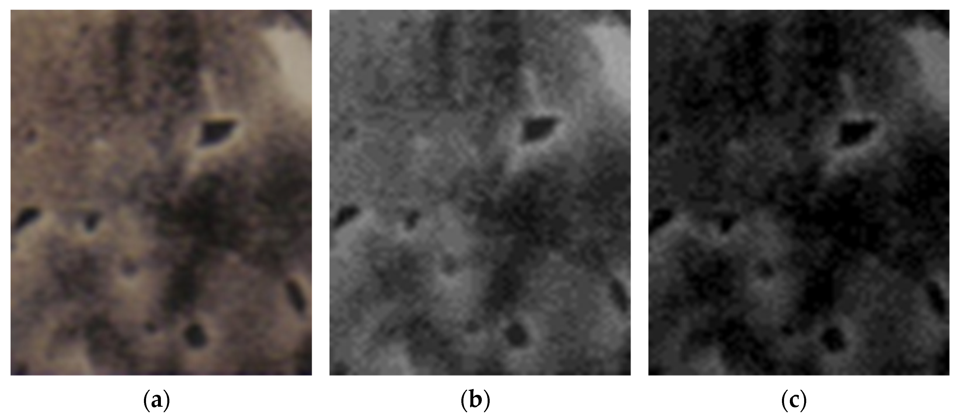
In Figure 7, the primary processing of the selected image 1 is depicted. This suite contains a set of three images, more specifically, from left to right, the original image (the portion in the yellow border), the grayscale version, as well as the grayscale version without luminance.
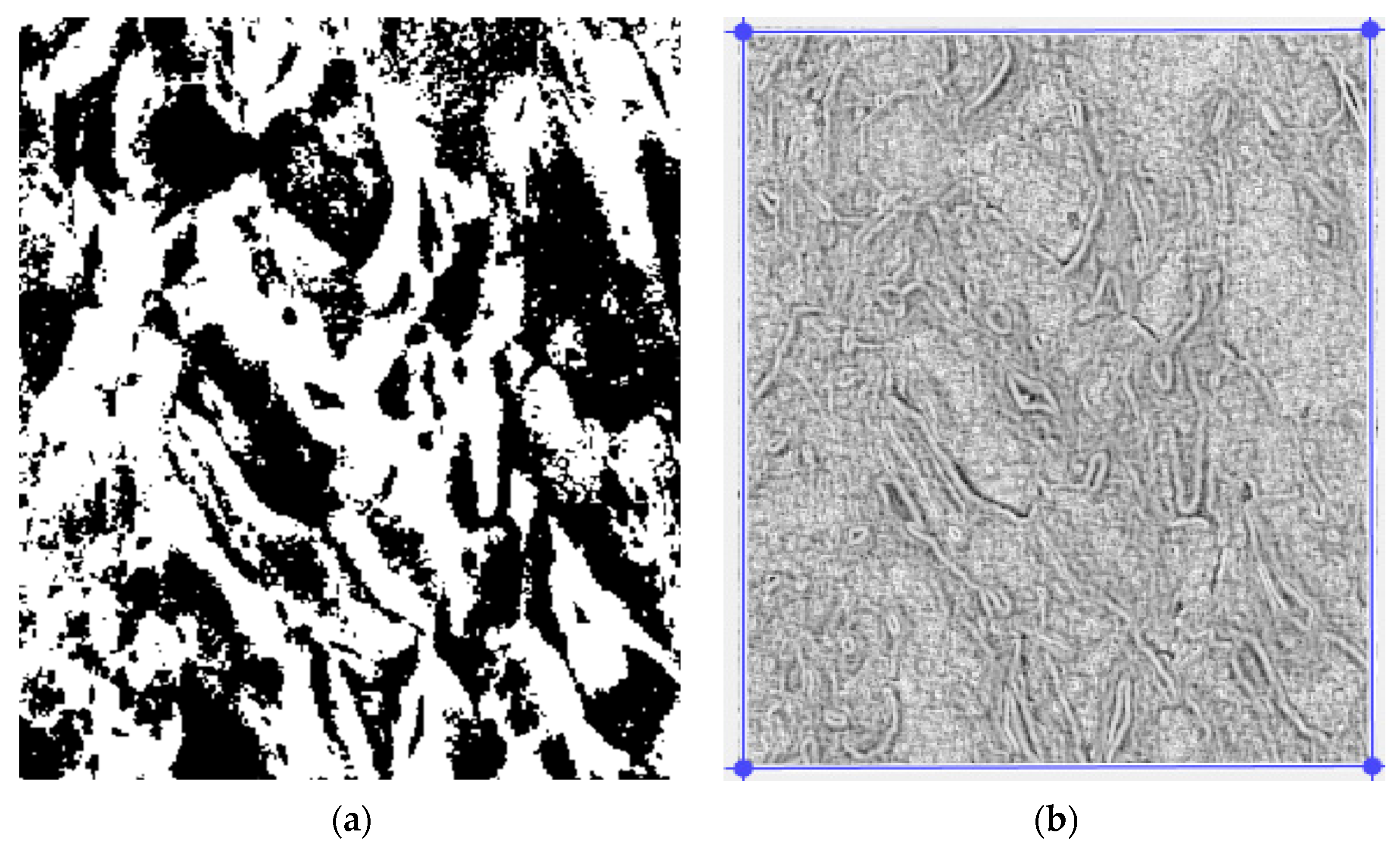
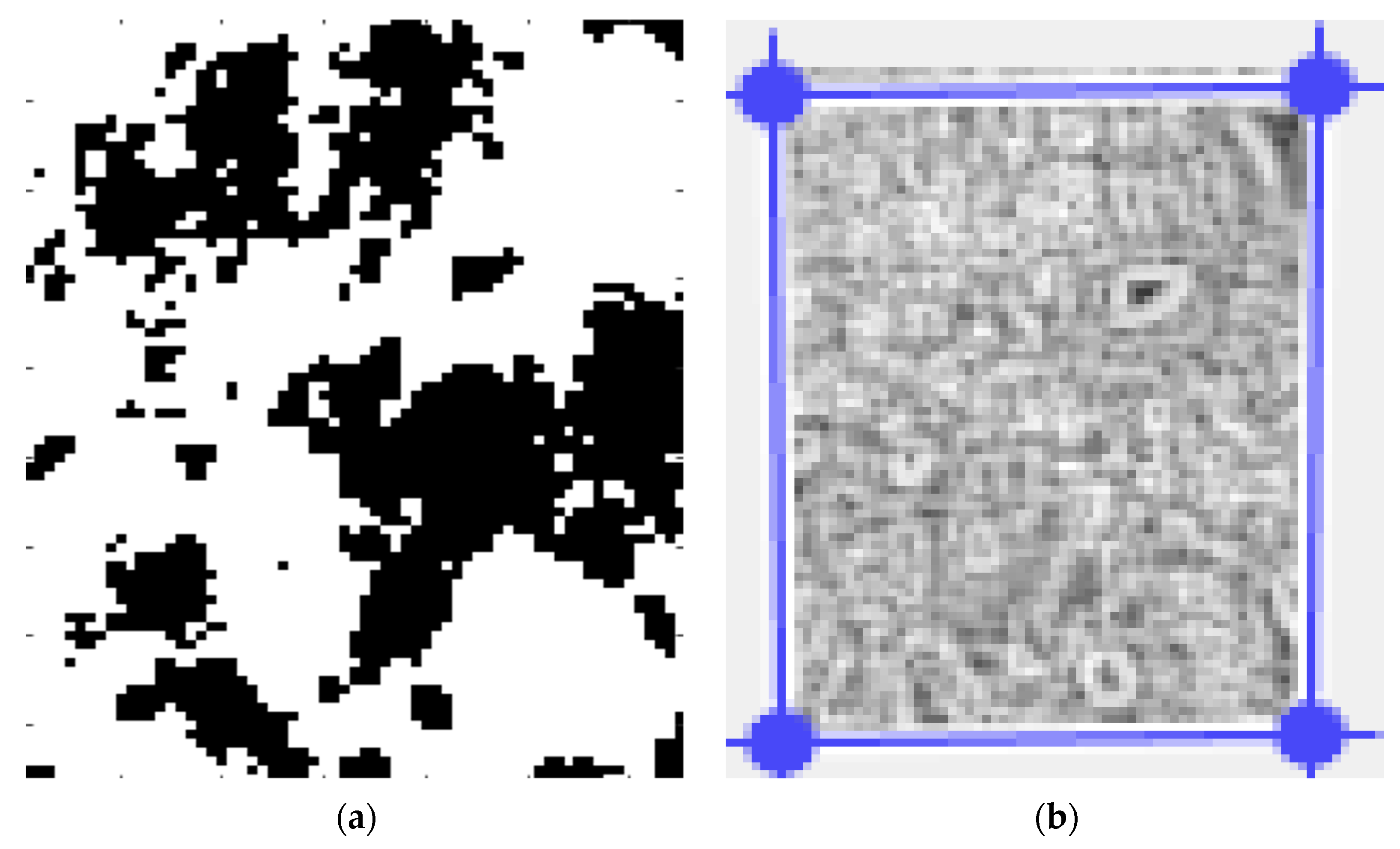
In Figure 8, the secondary processing of the selected image 1, including the binarized version and the application of the mask, are presented.
Following the numerical evaluations with the appropriate software of the selected image, the values of fractal dimension D = 1.8220, standard deviation , and lacunarity were obtained, as in Table 1.
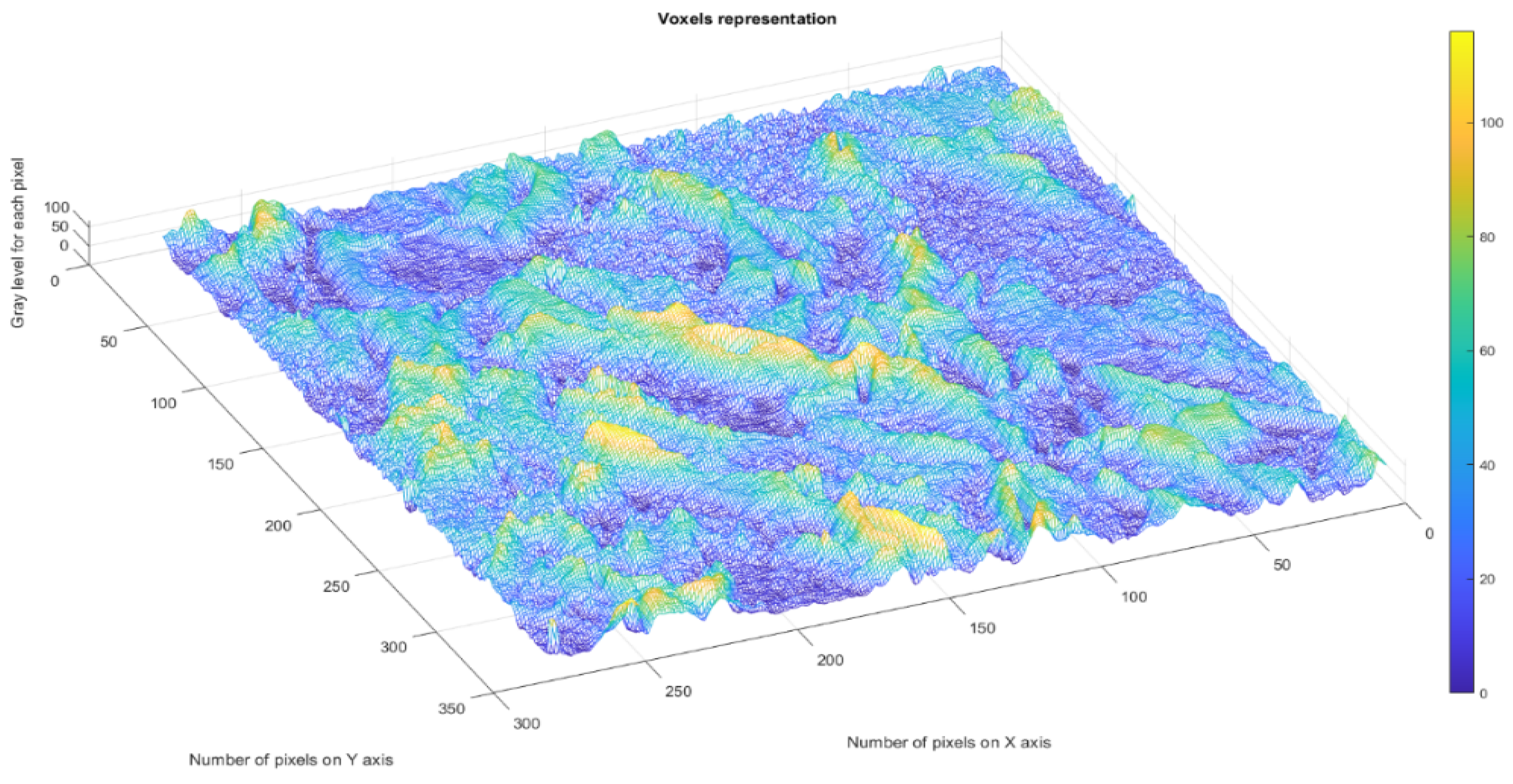
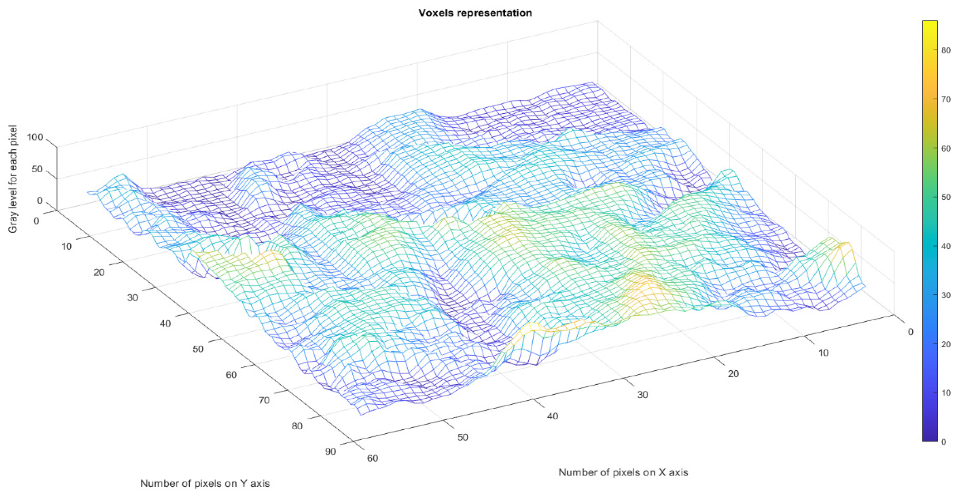
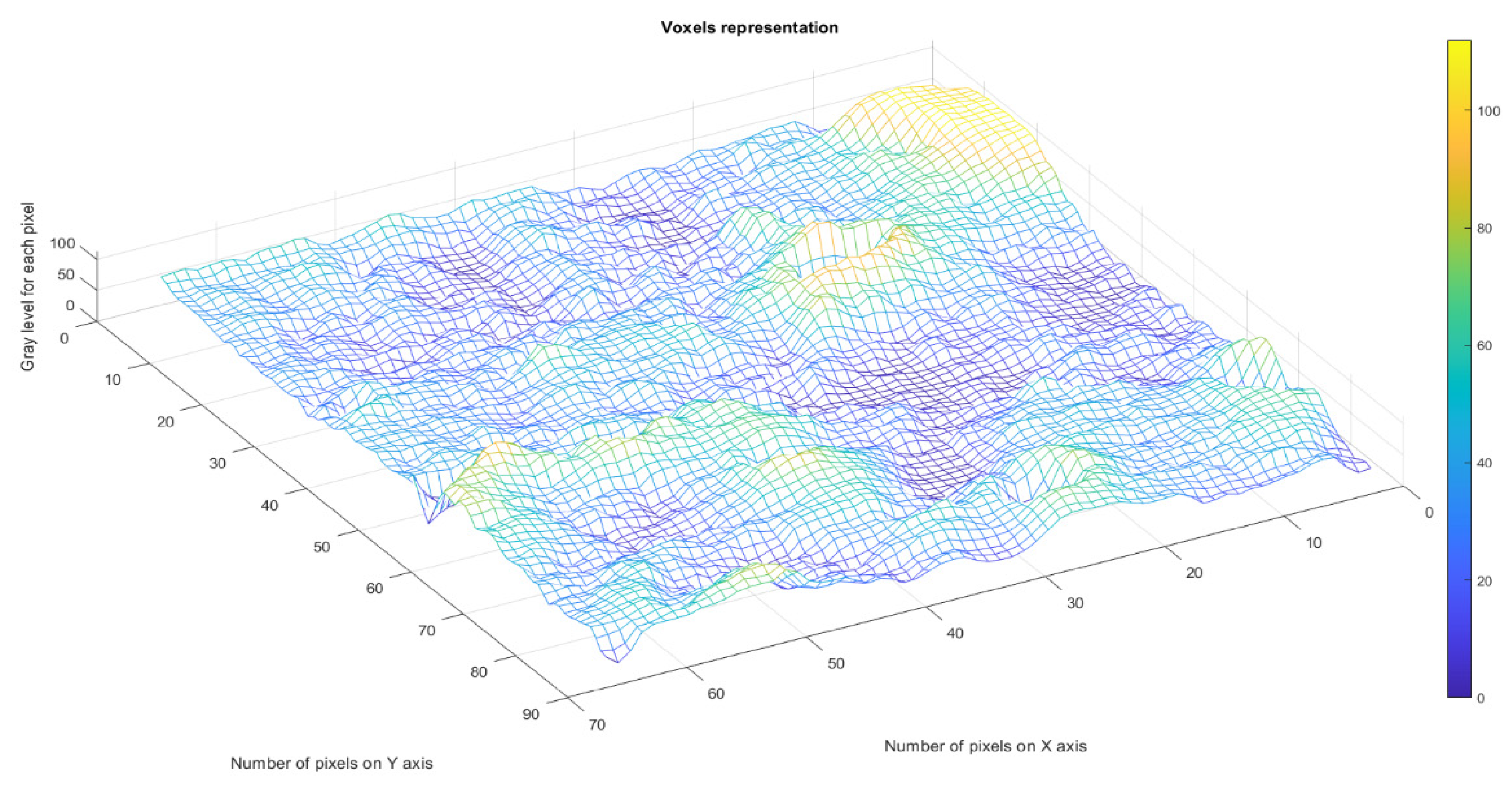
Figure 9 (see below) represents the three-dimensional graph of the voxel representation for image 1.
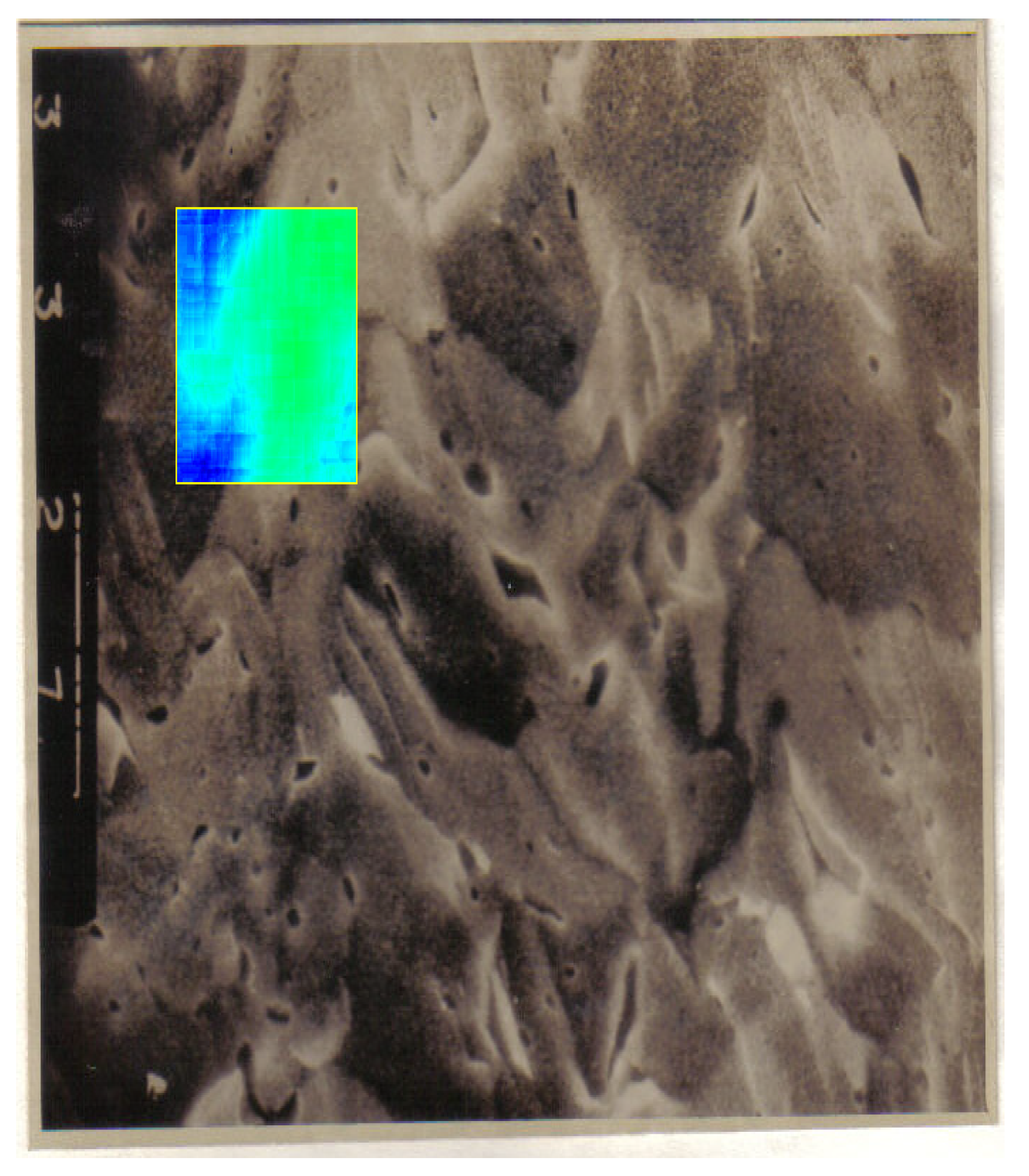
Step 2. The study of the selected zones images from the entire picture (according to Figure 10).
In Figure 10, we selected one distinct zone, the yellow rectangular frame zone, considered with different structures from a first visual analysis.
Figure 11 shows the attractor reconstruction [20] for the rectangle with yellow sides of normal area along with a considerable area with microcracks and prominent breakage, conformable to Figure 10. Both attractor reconstructions are presented. In embedding dimension 2, some points are observed, and in embedding dimension 3, some broken lines are noticed [16,17].
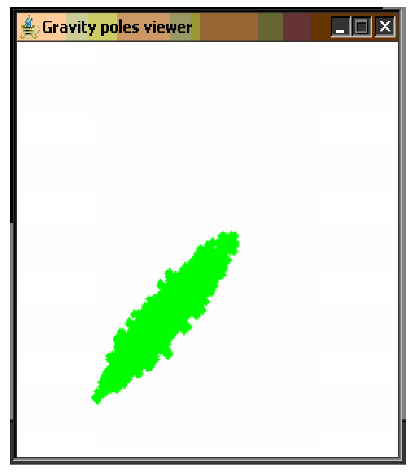
Further on, in Figure 12, the selection of the modified area with the application of WFDM for Figure 10 is presented. Staying on the same subject, the gravity poles of the modified area for Figure 10 are showcased in Figure 13.
Second, we study the time series generated by the picture associated with the selected modified area in Figure 14.
In Figure 14, the continuous green line placed horizontally represents the series average value over the entire time considered.
From Figure 15, we can determine the slope of the autocorrelation dimension versus the embedding dimension for the modified area (WFDM for Figure 10).
The graphic of the modified area (WFDM for Figure 10) autocorrelation, in Figure 15, representing the correlation dimension versus the embedding dimension, shows the slope computation. The correlation dimension versus the embedding dimension slope is 0.1455.
In Figure 16, the primary processing of the selected image 2 is depicted. This suite contains a set of three images, more specifically, from left to right, the original image (the portion in the yellow border), the grayscale version, as well as the grayscale version without luminance.
In Figure 17, the secondary processing of the selected image 2, including the binarized version and the application of the mask, are presented.
Following the numerical evaluations with the appropriate software of the selected image, the values of fractal dimension D = 1.7751, standard deviation , and lacunarity were obtained, as in Table 2.
Figure 18 (see below) represents the three-dimensional graph of the voxel representation for image 2.
Step 3. The study of the second chosen zone image according to Figure 19.
Figure 20 shows the attractor reconstruction [20] for the rectangle with yellow sides of a normal area along with a considerable area with microcracks and prominent breakage, conformable to Figure 19. Both attractor reconstructions are presented. In embedding dimension 2, some points are observed, and in embedding dimension 3, some broken lines are noticed [16,17].
Further on, in Figure 21, the selection of the modified area with the application of WFDM for Figure 19 is presented. Staying on the same subject, the gravity poles of the modified area for Figure 19 are showcased in Figure 22.
Second, we study the time series generated by the picture associated with the selected modified area in Figure 23.
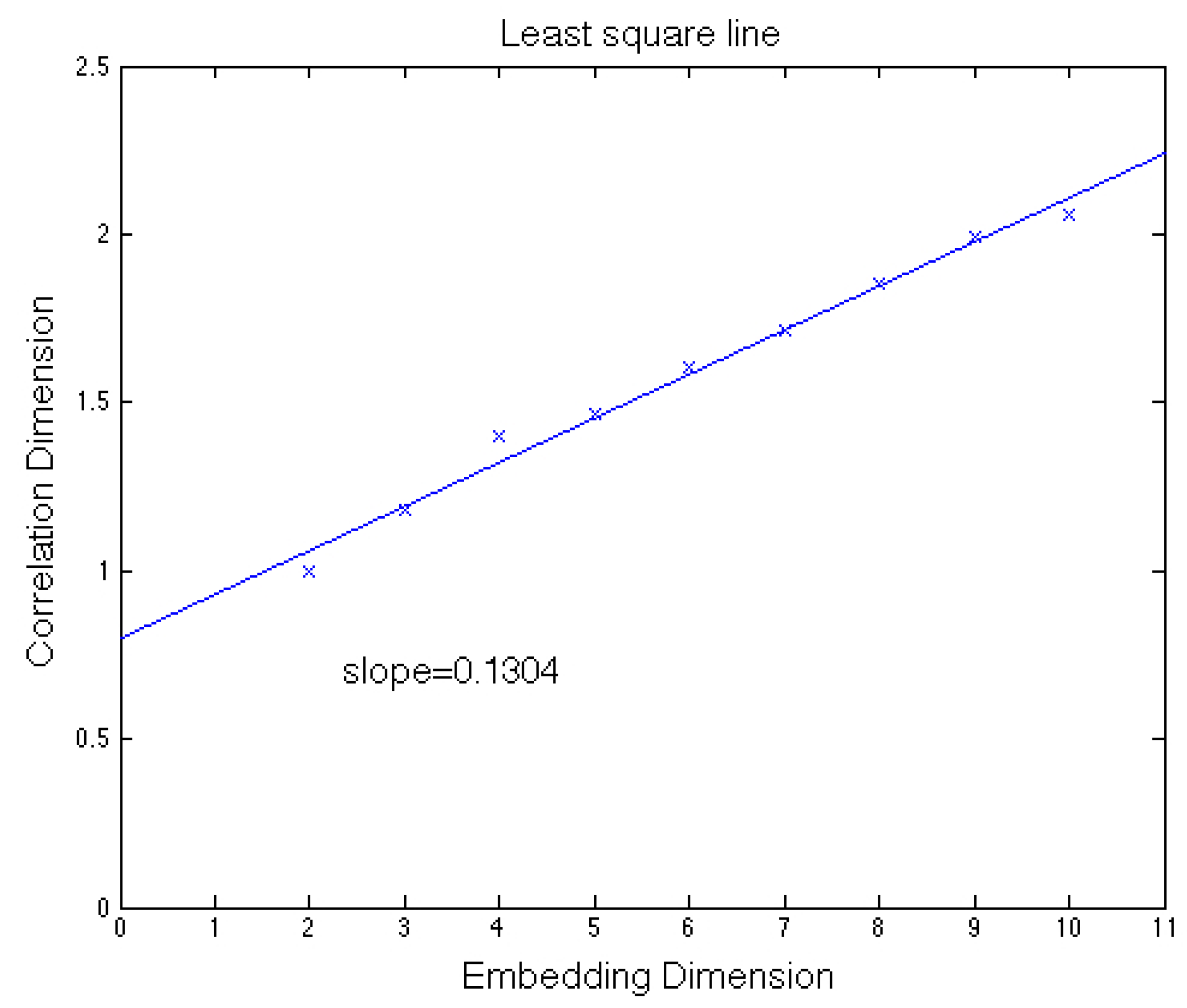
From Figure 23, we can determine the slope of the autocorrelation dimension versus the embedding dimension for the modified area (WFDM for Figure 19).
In Figure 23, the continuous green line placed horizontally represents the series average value over the entire time considered.
The graphic of the modified area (WFDM for Figure 19) autocorrelation, in Figure 24, representing the correlation dimension versus the embedding dimension, shows the slope computation. The correlation dimension versus the embedding dimension slope is 0.1304.
In Figure 25, the primary processing of the selected image 3 is depicted. This suite contains a set of three images, more specifically, from left to right, the original image (the portion in the yellow border), the grayscale version, as well as the grayscale version without luminance.
In Figure 26, the secondary processing of the selected image 3, including the binarized version and the application of the mask, is presented.
Following the numerical evaluations with the appropriate software of the selected image, the values of fractal dimension D = 1.8103, standard deviation , and lacunarity were obtained, as in Table 3.
Figure 27 (see below) represents the three-dimensional graph of the voxel representation for image 3.
Final Discussions
The substance of the work refers to the fact that the deformation of ceramics is different from that of metals and alloys, being small compared to that of metals, which means that they are fragile substances, unlike metals and alloys, which are ductile substances, characterized by consistent deformation at the same stress. In addition, the break develops at different levels of the loading load (tension); that is, the break in ceramics is made at a high level of stress, with an order of magnitude higher than the break in metals and alloys. We will continue to detail the differences in deformation and fracturing behaviour for ceramics and their connection with the fractal dimension of the image and its lacunarity.
We will present a mini explanation of the writing of this study below. The paper proposes a quantitative analysis of the SEM images of the fracture surface of UO2, using the fractal dimension of the image and its lacunarity. This information, obtained through the fractal analysis, is closely related to highlighting the type of fracture (brittle in our case) and the microcracks produced in the material. As can be seen, there is a direct connection with the microdeformations present on the image in the area without significant tearing of the material and a directly proportional increase in the lacunarity in the area with the rupture produced.
The method was explained above, but we also want to make a presentation of the things performed to put the method into operation. We have examined the fracture surfaces of two distinct areas with different microstructures to test for fractal behaviour. The zones are also differentiated by a simple visual observation, as they have distinct aspects due to the fact that one of the zones is unaffected by the breaking process, while the second zone is distinct due to the fact that it is a specific breaking zone.
A slit island analysis was used to determine the fractal dimension, D, of successively sectioned fracture surfaces. We found a correlation between increasing the fractional part of the fractal dimension and increasing toughness. In other words, as the toughness increases, the fracture surface increases in roughness. However, more than just a measure of roughness, the applicability of fractal geometry to a fracture implies a mechanism for generation of the fracture surface. The results presented here imply that brittle fracture is a fractal process; this means that we should be able to determine processes on the atomic scale by observing the macroscopic scale by finding the generator shape and the scheme for generation inherent in the fractal process. In addition, we attempt to relate the fractal dimension to fracture toughness. We also show that, in general, the fractal dimension increases with increasing fracture toughness.
4. Conclusions
The SEM micrographs of the fracture surface for a ceramic UO2 material, using the fractal analysis technique and time (spatial) series, have been investigated.
For the SEM picture analysis, a software application that generates a time series associated with the image, and then reconstructs the attractor and computes its autocorrelation dimension was developed.
The present study was carried out on a statistically sufficient number of SEM micrographs, treated according to the procedure of modified areas. To avoid augmentation in the article size, only one integral SEM picture has been presented from which one normal area (first zone) and another one corresponding to a modified area (second zone) have been selected.
The fractal dimension of the entire picture is D = 1.8220 ± 0.3440 and lacunarity is , and for the first zone (normal area), fractal dimension is D = 1.7751 ± 0.3363 and lacunarity is . For the second zone (modified area), the fractal dimension D = 1.8103 ± 0.3508 and lacunarity were obtained.
The average of the autocorrelation dimension for entire picture is 0.1023. The average of the autocorrelation dimension for the normal area of the first zone is 0.1455. The average of the autocorrelation dimension for the modified area of the second zone is 0.1304.
Author Contributions
Conceptualization, V.-P.P. and M.-A.P.; methodology, V.-P.P.; software, V.-A.P.; validation, V.-P.P., M.-A.P. and V.-A.P.; formal analysis, V.-P.P., M.-A.P. and V.-A.P.; investigation, V.-A.P. and M.-A.P.; resources, V.-A.P. and M.-A.P.; data curation, V.-A.P.; writing—original draft preparation, V.-P.P.; writing—review and editing, M.-A.P. and V.-P.P.; visualization, V.-A.P.; supervision, V.-P.P.; project administration, V.-P.P. All authors have read and agreed to the published version of the manuscript.
Funding
This research received no external funding.
Data Availability Statement
The data used to support the findings of this study cannot be accessed due to commercial confidentiality.
Acknowledgments
The co-authors M.A. Paun, V.A. Paun, and V.P. Paun thank Jenica Paun, for her continuous kind support.
Conflicts of Interest
The authors declare no conflict of interest.
References
- Lounsbury, M. The Natural Abundances of the Uranium Isotopes. Can. J. Chem. 1956, 34, 259–264. [Google Scholar] [CrossRef]
- Roberts, J.T.A.; Ueda, Y. Influence of Porosity on Deformation and Fracture of UO2. J. Am. Ceram. Soc. 1972, 55, 117–124. [Google Scholar] [CrossRef]
- Kapoor, K.; Ahmad, A.; Laksminarayana, A.; Hemanth Rao, G.V.S. Fracture properties of sintered UO2 ceramic pellets with duplex microstructure. J. Nucl. Mater. 2007, 366, 87–98. [Google Scholar] [CrossRef]
- Canon, R.F.; Roberts, J.T.A.; Beals, R.J. Deformation of UO2 at High Temperatures. J. Am. Ceram. Soc. 2006, 54, 105–112. [Google Scholar] [CrossRef]
- Moan, G.D.; Rudling, P. (Eds.) Zirconium in the Nuclear Industry, 13th International Symposium, ASTM-STP 1423; ASTM International: West Conshohocken, PA, USA, 2002; pp. 673–701. [Google Scholar]
- Kaddour, D.; Frechinet, S.; Gourgues, A.F.; Brachet, J.C.; Portier, L.; Pineau, A. Experimental determination of creep properties of Zirconium alloys together with phase transformation. Scr. Mater. 2004, 51, 515–519. [Google Scholar] [CrossRef] [Green Version]
- Brenner, R.; Béchade, J.L.; Bacroix, B. Thermal creep of Zr–Nb1%–O alloys: Experimental analysis and micromechanical modelling. J. Nucl. Mater. 2002, 305, 175–186. [Google Scholar] [CrossRef]
- Olteanu, M.; Paun, V.P.; Tanase, M. Fractal analysis of zircaloy-4 fracture surface, Conference on Equipments, Installations and Process Engineering. Rev. De Chim. 2005, 56, 97–100. [Google Scholar]
- Datseris, G.; Kottlarz, I.; Braun, A.P.; Parlitz, U. Estimating the fractal dimension: A comparative review and open source implementations. arXiv 2021, arXiv:2109.05937v1. [Google Scholar]
- Nichita, M.V.; Paun, M.A.; Paun, V.A.; Paun, V.P. Fractal Analysis of Brain Glial Cells. Fractal Dimension and Lacunarity. Univ. Politeh. Buchar. Sci. Bull. Ser. A Appl. Math. Phys. 2019, 81, 273–284. [Google Scholar]
- Bordescu, D.; Paun, M.A.; Paun, V.A.; Paun, V.P. Fractal Analysis of Neuroimagistics. Lacunarity Degree, a Precious Indicator in the Detection of Alzheimer’s Disease. Univ. Politeh. Buchar. Sci. Bull. Ser. A Appl. Math. Phys. 2018, 80, 309–320. [Google Scholar]
- Peitgen, H.-O.; Jurgens, H.; Saupe, D. Chaos and Fractals. In New Frontiers of Science; Springer: Berlin/Heidelberg, Germany, 1992. [Google Scholar]
- Mandelbrot, B.B.; Passoja, D.E.; Paullay, A.J. Fractal character of fracture surfaces of metals. Nature 1984, 308, 721–722. [Google Scholar] [CrossRef]
- Mandelbrot, B. Fractal Geometry of Nature; Freeman: New York, NY, USA, 1983; pp. 25–57. [Google Scholar]
- Paun, V.P. Fractal surface analysis of Zircaloy-4 SEM micrographs using the time-series method. Cent. Eur. J. Phys. 2009, 7, 264–269. [Google Scholar]
- Takens, F. Detecting strange attractors in turbulence. Lect. Notes Math. 1981, 898, 366–381. [Google Scholar]
- Takens, F. On the numerical determination of the dimension of an attractor. In Dynamical Systems and Bifurcations; Braaksma, B.L.J., Broer, H.W., Takens, F., Eds.; Springer: Berlin/Heidelberg, Germany, 1985; pp. 99–106. [Google Scholar]
- Xu, L.; Shi, Y. Notes on the Global Attractors for Semigroup. Int. J. Mod. Nonlinear Theory Appl. 2013, 2, 219–222. [Google Scholar] [CrossRef] [Green Version]
- Sauer, T.; Yorke, J.; Casdagli, M. Embedology. J. Stat. Phys. 1991, 65, 579–616. [Google Scholar] [CrossRef]
- Passoja, D.E.; Psioda, J.A. Fractography in Materials Science; ASTM International: West Conshohocken, PA, USA, 1981; pp. 335–386. [Google Scholar]
- Mattfeldt, T. Nonlinear deterministic analysis of tissue texture: A stereological study on mastopathic and mammary cancer tissue using chaos theory. J. Microsc. 1997, 185, 47–66. [Google Scholar] [CrossRef] [PubMed]
- Thompson, J.M.T.; Stewart, H.B. Nonlinear Dynamics and Chaos; John Wiley and Sons: Hoboken, NJ, USA, 1986. [Google Scholar]
- Horovistiz, A.; de Campos, K.A.; Shibata, S.; Prado, C.C.; de Oliveira Hein, L.R. Fractal characterization of brittle fracture in ceramics under mode I stress loading. Mater. Sci. Eng. A 2010, 527, 4847–4850. [Google Scholar] [CrossRef]
- Falconer, K. Fractal Geometry: Mathematical Foundations and Applications, 3rd ed.; John Wiley & Sons, Ltd.: Chichester, UK, 2014. [Google Scholar]
- Nichita, M.V.; Paun, M.A.; Paun, V.A.; Paun, V.P. Image Clustering Algorithms to Identify Complicated Cerebral Diseases. Description and Comparaisons. IEEE Access 2020, 8, 88434–88442. [Google Scholar] [CrossRef]
- Postolache, P.; Borsos, Z.; Paun, V.A.; Paun, V.P. New Way in Fractal Analysis of Pulmonary Medical Images. Univ. Politeh. Buchar. Sci. Bull. Ser. A Appl. Math. Phys. 2018, 80, 313–322. [Google Scholar]
- Scott, D.W. Statistics: A Concise Mathematical Introduction for Students, Scientists, and Engineers; John Wiley & Sons, Inc.: Hoboken, NJ, USA, 2020. [Google Scholar]
Figure 1.
Original image and a selected area.

Figure 2.
Attractor reconstruction.

Figure 3.
The time series generated by the selected area in Figure 1.
Figure 3.
The time series generated by the selected area in Figure 1.

Figure 4.
The selection of the modified area (according to WFDM).

Figure 5.
The gravity poles of the modified area.

Figure 6.
The autocorrelation dimension versus the embedding dimension for the modified area.

Figure 7.
Primary processing of the selected image 1: (a) original image (the portion in the yellow border); (b) the grayscale version; and (c) the grayscale version without luminance.
Figure 7.
Primary processing of the selected image 1: (a) original image (the portion in the yellow border); (b) the grayscale version; and (c) the grayscale version without luminance.

Figure 8.
Secondary processing of the selected image 1: (a) binarized version; (b) application of the mask. A threshold of 25 was used for binarization.
Figure 8.
Secondary processing of the selected image 1: (a) binarized version; (b) application of the mask. A threshold of 25 was used for binarization.

Figure 9.
Voxels representation for image 1.

Figure 10.
The first distinct zone selection.

Figure 11.
Attractor reconstruction.

Figure 12.
The selection of the modified area (WFDM) for Figure 10.
Figure 12.
The selection of the modified area (WFDM) for Figure 10.

Figure 13.
The gravity poles of the modified area for Figure 10.
Figure 13.
The gravity poles of the modified area for Figure 10.

Figure 14.
The time series generated by the selected modified area for Figure 10.
Figure 14.
The time series generated by the selected modified area for Figure 10.

Figure 15.
The autocorrelation dimension versus the embedding dimension for the modified area.

Figure 16.
Primary processing of the selected image 2: (a) original image (the portion in the yellow border); (b) the grayscale version; and (c) the grayscale version without luminance.
Figure 16.
Primary processing of the selected image 2: (a) original image (the portion in the yellow border); (b) the grayscale version; and (c) the grayscale version without luminance.

Figure 17.
Secondary processing of the selected image 2: (a) binarized version; (b) application of the mask. A threshold of 25 was used for binarization.
Figure 17.
Secondary processing of the selected image 2: (a) binarized version; (b) application of the mask. A threshold of 25 was used for binarization.

Figure 18.
Voxels representation for image 2.

Figure 19.
Image and a selected area for the second distinct zone.

Figure 20.
Attractor reconstruction.

Figure 21.
The selection of the modified area (WFDM) for Figure 19.
Figure 21.
The selection of the modified area (WFDM) for Figure 19.

Figure 22.
The gravity poles of the modified area for Figure 19.
Figure 22.
The gravity poles of the modified area for Figure 19.

Figure 23.
The time series generated by the selected modified area for Figure 19.
Figure 23.
The time series generated by the selected modified area for Figure 19.

Figure 24.
The autocorrelation dimension versus the embedding dimension for the modified area.

Figure 25.
Primary processing of the selected image 3: (a) original image (the portion in the yellow border); (b) the grayscale version; and (c) the grayscale version without luminance.
Figure 25.
Primary processing of the selected image 3: (a) original image (the portion in the yellow border); (b) the grayscale version; and (c) the grayscale version without luminance.

Figure 26.
Secondary processing of the selected image 3: (a) binarized version; (b) application of the mask. A threshold of 25 was used for binarization.
Figure 26.
Secondary processing of the selected image 3: (a) binarized version; (b) application of the mask. A threshold of 25 was used for binarization.

Figure 27.
Voxels representation for image 3.


Table 1.
Calculation of fractal parameters.
| Name | Fractal Dimension | Standard Deviation | Lacunarity |
|---|---|---|---|
| Image 1 | 1.8220 | ±0.3440 | 0.0357 |
Table 2.
Calculation of fractal parameters.
| Name | Fractal Dimension | Standard Deviation | Lacunarity |
|---|---|---|---|
| Image 2 | 1.7751 | ±0.3363 | 0.0359 |
Table 3.
Calculation of fractal parameters.
| Name | Fractal Dimension | Standard Deviation | Lacunarity |
|---|---|---|---|
| Image 3 | 1.8103 | ±0.3508 | 0.0375 |
Publisher’s Note: MDPI stays neutral with regard to jurisdictional claims in published maps and institutional affiliations. |
© 2022 by the authors. Licensee MDPI, Basel, Switzerland. This article is an open access article distributed under the terms and conditions of the Creative Commons Attribution (CC BY) license (https://creativecommons.org/licenses/by/4.0/).
Share and Cite
MDPI and ACS Style
Paun, M.-A.; Paun, V.-A.; Paun, V.-P. Spatial Series and Fractal Analysis Associated with Fracture Behaviour of UO2 Ceramic Material. Fractal Fract. 2022, 6, 595. https://doi.org/10.3390/fractalfract6100595
AMA Style
Paun M-A, Paun V-A, Paun V-P. Spatial Series and Fractal Analysis Associated with Fracture Behaviour of UO2 Ceramic Material. Fractal and Fractional. 2022; 6(10):595. https://doi.org/10.3390/fractalfract6100595
Chicago/Turabian StylePaun, Maria-Alexandra, Vladimir-Alexandru Paun, and Viorel-Puiu Paun. 2022. "Spatial Series and Fractal Analysis Associated with Fracture Behaviour of UO2 Ceramic Material" Fractal and Fractional 6, no. 10: 595. https://doi.org/10.3390/fractalfract6100595