Synchronizability of Multilayer Directed Dutch Windmill Networks

Abstract

This paper investigates the synchronizability of multilayer directed Dutch windmill networks with the help of the master stability function method. Here, we propose three types of multilayer directed networks with different linking patterns, namely, inter-layer directed networks (Networks-A), intra-layer directed networks (Networks-B), and hybrid directed networks (Networks-C), and rigorously derive the analytical expressions of the eigenvalue spectrum on the basis of their supra-Laplacian matrix. It is found that network structure parameters (such as the number of layers and nodes, the intra-layer and the inter-layer coupling strengths) have a significant impact on the synchronizability in the case of the two typical synchronized regions. Finally, in order to confirm that the theoretical conclusions are correct, simulation experiments of multilayer directed network are delivered.

1. Introduction

The emergence of small-world networks and scale-free networks [1,2] has been the beginning of a large amount of significant research outcomes that have been obtained in complex networks. They are widely used in information networks, biological networks, neural networks, social networks, power grids, and other frontier fields [3,4,5,6,7]. It is recognized that most networks in reality do not exist independently but are composed of multiple networks coupling and interacting with each other [8,9]. With the development of network theory, many innovative advances in the field of multilayer networks have been gained, for instance, the control and synchronization of systems [10,11,12,13,14], the diffusion and superdiffusion in networks [15,16,17], consensus problems and robustness of multilayer networks [18,19,20].

Synchronization, such as clapping in unison and chorus cicadas, is a significant collective behavior on complex networks. Previous research has been conducted on different synchronization effects of single network, such as complete synchronization, generalized synchronization, phase synchronization, and finite-time synchronization [21,22,23,24]. Based on the asymptotic analysis, Fan et al. [25] provided some criteria of synchronization about complex dynamical networks that allowed us to infer the behavior of dynamics. In terms of the master stability function method, Xu et al. [26] focused on the two-layer star networks and studied that network parameters are important roles in affecting the synchronization capabilities of multilayer networks with more than two layers. Zhang et al. [27] derived an analytic expression for the eigenvalue spectrum of a multiplex k-nearest neighbor coupled network, and discussed the relationship between structure parameters and the synchronizability. Li et al. [28] analyzed the synchronization of dumbbell networks with two layers, comparing two interlink patterns between layers, and found that the coupling patterns is a discussion point for exploring the multilayer networks. It is necessary to study more types of networks with more than two layers to study the synchronizability. There are many regular and typical network structures; windmill network is one of them, and common windmill network types are the Dutch windmill network [29] and the French windmill network. Estrada [30] proved that the clustering coefficient was divergent with the network size increasing to infinity, as well as the transitivity. In addition, Kooij [31] considered three generalizations of windmill graphs, and studied topological properties and eigenvalue spectrum for all three types. Sun et al. [32] employed the first two generalized noisy windmill networks to study the consensus and robustness, quantifying all eigenvalues of their matrixes, about the leaderless model and the leader–follower model. Zhu et al. [33] derived all eigenvalues of two different variable coupling multilayer windmill-type network models and gave numerical experiments to demonstrate that the synchronizability can be improved by changing the structural parameters. Research on windmill networks have been dedicated to network structures and synchronizability with only one layer, and there are relatively few results of multilayer networks which are closer to the actual situation. Moreover, systems in the real world are more likely to be weighted directed networks. The direction and coupling weights make it difficult to obtain analytical expressions of eigenvalues of the Laplacian matrix.

Summarizing the above findings, it was found that the master stability function (MSF) method [34], used in this paper, is a particularly useful approach to investigate complex networks. We have the following innovations about multilayer directed Dutch windmill networks.

(1)

We propose three kinds of multilayer directed Dutch windmill networks with different inter-layer and intra-layer connection pattern.

(2)

With the help of graph spectra methods, we obtain the supra-Laplace matrix based on the structure of these networks. It is obvious that the expressions for the eigenvalues are expressed.

(3)

It is worth exploring to know that the synchronizability is associated with topological structure parameters (for example, network size N, the number of layers M, intra-layer coupling weights a, and inter-layer coupling weights d), which is studied by MSF when the synchronized regions are bounded and unbounded.

(4)

Under the given initial conditions, numerical experiments are conducted to show that the state trajectory of nodes could achieve synchronization. In addition, we verify the correctness of analytical results and offer a theoretical support for strengthening their ability of reaching synchronization.

This paper has the following section arrangement. Section 2 gives essential preliminaries and the models of multilayer directed networks. The eigenvalue spectrum of Networks-A, B, and C are rigorously derived in Section 3 and numerical examples are performed in Section 4 for interpreting the realizability of theoretical findings. Lastly, Section 5 draws the summarized comments.

2. Preliminaries

2.1. The Dynamic Models of Multilayer Networks

For a multilayer network consisting of M layers and N nodes each layer, the dynamics of $x_i^{\alpha }$ can be described as [35]:

$$\frac{d{x}_i^{\alpha }}{dt}=f\left(x_i^{\alpha }\right)-a\sum _{j=1}^N{w}_{ij}^{\alpha }{\Gamma }_1\left(x_j^{\alpha }\right)-d\sum _{\beta =1}^M{d}_i^{\alpha \beta }{\Gamma }_2\left(x_i^{\beta }\right),$$

(1)

where $x_i^{\alpha }\in {\mathcal{R}}^s$ is the state of the $i$th node in the $\alpha$th layer, $1\le i\le N, 1\le \alpha \le M$. $f:{\mathcal{R}}^s\to {\mathcal{R}}^s$ is a nonlinear vector function governing the dynamics of the $i$th node in the $\alpha$th. a denotes intra-layer coupling strength inside each layer and ${\Gamma }_1:{\mathcal{R}}^s\to {\mathcal{R}}^s$ is the corresponding inner coupling function. d respects inter-layer coupling strength between replicas and ${\Gamma }_2:{\mathcal{R}}^s\to {\mathcal{R}}^s$ is the inter-layer coupling function. For simplicity, let ${\Gamma }_1\left(x_j^{\alpha }\right)={\Gamma }_1{x}_j^{\alpha }$, ${\Gamma }_2\left(x_i^{\beta }\right)={\Gamma }_2{x}_i^{\beta }$ and ${\Gamma }_1={\Gamma }_2=\Gamma$. For an undirected network, if there is an edge connecting the $i$th node and the $j$th node in the $\alpha$th layer ($i\ne j$), $w_{ij}^{\alpha }=-1$, otherwise $w_{ij}^{\alpha }=0$ with $w_{ii}^{\alpha }=-{\sum }_{j=1,j\ne i}^N{w}_{ij}^{\alpha }$. Thus, the intra-layer Laplacian matrix of the $\alpha$th layer is described as $L^{\left(\alpha \right)}=\left(a{w}_{ij}^{\alpha }\right)\in {\mathcal{R}}^{N\times N}$. Similarly, if there is a link connecting the $i$th node and its replica across layers, $d_i^{\alpha \beta }=-1$, otherwise $d_i^{\alpha \beta }=0$, and $d_i^{\alpha \alpha }=-{\sum }_{\beta =1,\beta \ne \alpha }^M{d}_i^{\alpha \beta }$. $L^I=\left(d{d}_i^{\alpha \beta }\right)\in {\mathcal{R}}^{M\times M}$ is the inter-layer Laplacian matrix. In particular, when a node is unidirectionally connected to its other replica nodes, $L^I$ may be an upper triangular matrix or a lower triangular matrix.

For simplicity, we denote

$$\begin{array}{cc}\hfill x^{\left(\alpha \right)}=\left(\begin{array}{c}{x}_1^{\alpha }\\ x_2^{\alpha }\\ ⋮\\ x_N^{\alpha }\end{array}\right),& X=\left(\begin{array}{c}{x}^{\left(1\right)}\\ x^{\left(2\right)}\\ ⋮\\ x^{\left(M\right)}\end{array}\right),\hfill \\ \hfill \tilde{f}\left(x^{\left(\alpha \right)}\right)=\left(\begin{array}{c}f\left(x_1^{\alpha }\right)\\ f\left(x_2^{\alpha }\right)\\ ⋮\\ f\left(x_N^{\alpha }\right)\end{array}\right),& F\left(x\right)=\left(\begin{array}{c}\tilde{f}\left(x^{\left(1\right)}\right)\\ \tilde{f}\left(x^{\left(2\right)}\right)\\ ⋮\\ \tilde{f}\left(x^{\left(M\right)}\right)\end{array}\right).\hfill \end{array}$$

(2)

It follows that Equation (1) has a concise matrix form, namely,

$$\dot{X}=F\left(X\right)-\left(({\mathcal{L}}^{\mathcal{L}}+{\mathcal{L}}^{\mathcal{I}})\otimes \Gamma \right)X,$$

(3)

where ⨂ is the Kronecker product. The intra-layer supra-Laplacian matrix ${\mathcal{L}}^{\mathcal{L}}$, reflecting the coupling relationships within each layer, is the direct sum of $L^{\left(\alpha \right)}$. In detail,

$${\mathcal{L}}^{\mathcal{L}}=\left(\begin{array}{cccc}{L}^{\left(1\right)}& 0& \cdots & 0\\ 0& L^{\left(2\right)}& \cdots & 0\\ ⋮& ⋮& \ddots & ⋮\\ 0& 0& \cdots & L^{\left(M\right)}\end{array}\right)=\underset{\alpha =1}{\overset{M}{\oplus }}{L}^{\left(\alpha \right)}.$$

(4)

${\mathcal{L}}^{\mathcal{I}}=L_I\otimes I_N$ represents the links across layers, where $I_N$ stands for the identity matrix of N-dimensional. The supra-Laplacian matrix $\mathcal{L}$ of the multilayer network is replaced by ${\mathcal{L}}^{\mathcal{I}}$ and ${\mathcal{L}}^{\mathcal{L}}$ [36]:

$$\mathcal{L}={\mathcal{L}}^{\mathcal{I}}+{\mathcal{L}}^{\mathcal{L}}.$$

(5)

2.2. Synchronized Regions of Multilayer Networks

$\mathcal{L}$ represents the supra-Laplacian matrix of multilayer networks, having one zero eigenvalue and all other eigenvalues are positive: $0={\lambda }_1<{\lambda }_2\le \cdots \le {\lambda }_{max}$. Based on the concept of MSF, it is general to group the synchronized region $\left(SR\right)$ in four cases as follows [37]:

(1)

$SR=({\alpha }_1,+\infty )$ denotes the unbounded synchronized region, where ${\alpha }_1$ is a finite positive real number. If ${\lambda }_2$ is greater than the threshold ${\alpha }_1$, which portrays the synchronizability of the network, and all larger eigenvalues will be included in the $SR$. Therefore, the larger ${\lambda }_2$ is, the stronger the synchronizability is.

(2)

$SR=({\alpha }_1,{\alpha }_2)$ denotes the bounded synchronized region, where ${\alpha }_1$ and ${\alpha }_2$ are finite positive real numbers and ${\alpha }_1<{\alpha }_2$. In order to make all values fall within the synchronization field, it is obvious that after deformation the eigenratio can be found, which satisfies $r={\lambda }_{max}/{\lambda }_2<{\alpha }_2/{\alpha }_1$. Moreover, the lower ratio r demonstrates higher capability of achieving synchronization.

(3)

The synchronized region is the union of several intervals. For instance, in the form of $SR=({\alpha }_1,{\alpha }_2)\cup ({\alpha }_3,{\alpha }_4)$. If all ${\lambda }_i$ are restricted to the range of $SR$, then the synchronization can be realized and the states of all nodes in the network converge to a steady state.

(4)

The synchronized region is an empty set. In this case, synchronization is not possible regardless of the variation of the coupling function and coupling strength.

Which type of synchronization domain a network belongs to is primarily decided by the inner coupling function $\Gamma$ and dynamics functions f. Here, the study of the first two scenarios, the bounded and unbounded synchronous regions, is representative. When it comes to the synchronizability, it is of vital simplicity for us to derive the second smallest eigenvalue and eigenratio of its Laplacian matrix for directed Dutch windmill networks.

2.3. Multilayer Directed Dutch Windmill Networks

This paper gives the eigenvalue expression and studies the synchronizability for multilayer directed Dutch windmill networks. It can be supposed simply that multiplex networks has M layers and the network size N is identical for each layer. One possible type of inter-layer connections means the each node is one-to-one connected into its replicas that are not on the same layer. Generally, a windmill graph contains $\eta$ copies of the complete network $K_k$ [38] and windmill networks are rule networks. In this article, the nodes on each layer, related to the multilayer directed Dutch windmill networks, satisfies $N=2\eta$ + 1. It is quite easy to see that N is proportional to $\eta$.

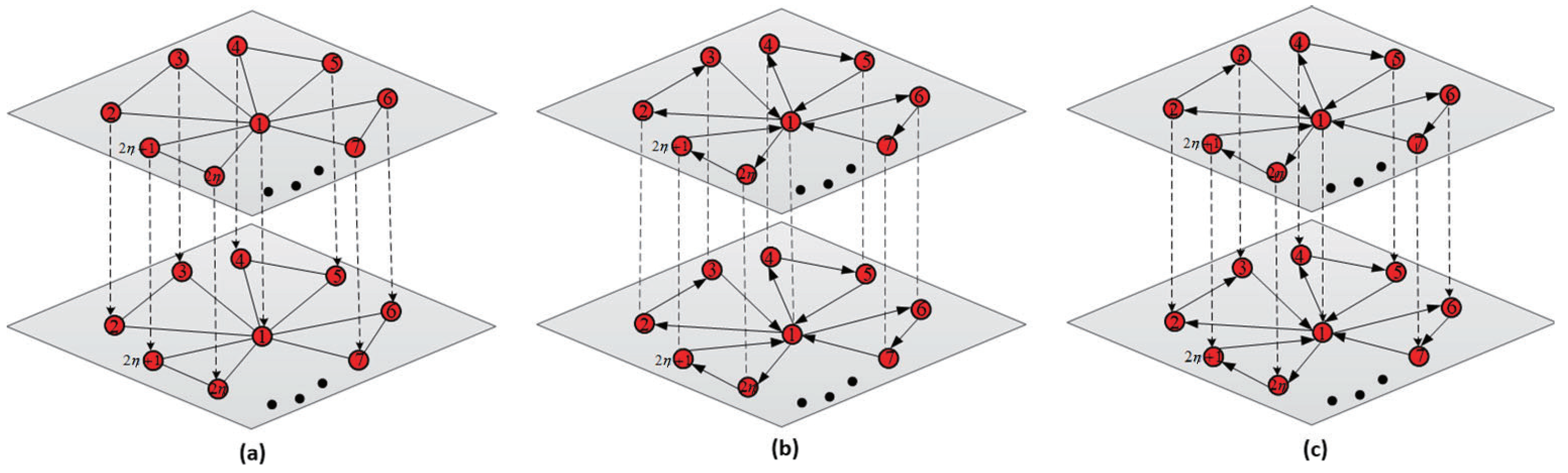
The two interlayer connection methods of each node, undirected one-to-one connection and unidirectional one-to-one coupling, are considered. For the former, undirected links, or bidirectional, exist between the nodes of each two layers. For the latter, nodes within a layer are unidirectionally connected to replicated nodes in other layers, without duplicating. Moreover, there are different types of linking patterns, occurring among nodes within each layer: directed with the same sequence and undirected. Because of the aim of studying the synchronizability of directed networks, three kinds of multilayer directed Dutch windmill networks, multilayer inter-layer directed Dutch windmill networks (Networks-A), multilayer intra-layer directed Dutch windmill networks (Networks-B), and multilayer both inter-layer and intra-layer directed Dutch windmill networks (Networks-C) are defined. For Networks-A, the inter-layer interconnection method is unidirectional coupling between replica nodes, and the intra-layer interconnection method is undirected. On the contrary, Networks-B means that the nodes are directionally connected in the same sequence within each layer but undirected between replica nodes across layers. In addition, Networks-C is a combination of Networks-A and Networks-B which is directed connected within layers and unidirectional coupling between layers. Figure 1 shows the corresponding structure with two layers.

To make convenient the following theoretical derivation, useful lemmas are presented as follows:

Lemma 1

([39]). If $A_{ii}$ is a square matrix, $i=1,\dots ,k$, then

$$\left|\begin{array}{cccc}{A}_{11}& A_{12}& \cdots & A_{1k}\\ 0& A_{22}& \cdots & A_{2k}\\ ⋮& ⋮& \ddots & ⋮\\ 0& 0& \cdots & A_{kk}\end{array}\right|=|A_{11}|·|A_{22}|\cdots |A_{kk}|.$$

(6)

Lemma 2

([40]). Let S be a square matrix and T have the same size, then

$${\left|\begin{array}{cccc}S& T& \cdots & T\\ T& S& \cdots & T\\ ⋮& ⋮& \ddots & ⋮\\ T& T& \cdots & S\end{array}\right|}_{M\times M}={|S-T|}^{M-1}·|S+(M-1)T|.$$

(7)

3. The Synchronizability of Multilayer Directed Dutch Windmill Networks

3.1. The Eigenvalues of Networks-A

This section considers the generalized Networks-A with M layers each is made up of N nodes whose diagram is shown in Figure 2. The corresponding supra-Laplacian matrix is obtained, expressed as ${\mathcal{L}}_{\mathcal{A}}$:

$${\mathcal{L}}_{\mathcal{A}}={\left(\begin{array}{cccc}a{L}_A+(M-1)d{I}_N& -d{I}_N& \cdots & -d{I}_N\\ 0& a{L}_A+(M-2)d{I}_N& \cdots & -d{I}_N\\ ⋮& ⋮& \ddots & ⋮\\ 0& 0& \cdots & a{L}_A\end{array}\right)}_{M\times M},$$

(8)

where

$$L_A={\left(\begin{array}{cccccccc}2\eta & -1& -1& -1& -1& \cdots & -1& -1\\ -1& 2& -1& 0& 0& \cdots & 0& 0\\ -1& -1& 2& 0& 0& \cdots & 0& 0\\ ⋮& ⋮& ⋮& ⋮& ⋮& \ddots & ⋮& ⋮\\ -1& 0& 0& 0& 0& \cdots & 2& -1\\ -1& 0& 0& 0& 0& \cdots & -1& 2\end{array}\right)}_{N\times N}.$$

In accordance with Lemma 1 introduced earlier, the characteristic polynomial of ${\mathcal{L}}_A$ can be given:

$$\begin{array}{cc}\hfill & |\lambda I_{MN}-{\mathcal{L}}_A|\hfill \\ \hfill =& \left|\begin{array}{cccc}[\lambda -(M-1)d]I_N-a{L}_A& -d{I}_N& \cdots & -d{I}_N\\ 0& [\lambda -(M-2)d]I_N-a{L}_A& \cdots & -d{I}_N\\ ⋮& ⋮& \ddots & ⋮\\ 0& 0& \cdots & \lambda I_N-a{L}_A\end{array}\right|\hfill \\ \hfill & |[\lambda -(M-1)d]I_N-a{L}_A|·\left|\begin{array}{ccc}[\lambda -(M-2)d]I_N-a{L}_A& \cdots & -d{I}_N\\ ⋮& \ddots & ⋮\\ 0& \cdots & \lambda I_N-a{L}_A\end{array}\right|\hfill \\ \hfill =& |\lambda I_N-a{L}_A|·|(\lambda -d)I_N-a{L}_A|·|(\lambda -2d)I_N-a{L}_A|\hfill \\ \hfill & \cdots |(\lambda -(M-2)d)I_N-a{L}_A|·|(\lambda -(M-1)d)I_N-a{L}_A|.\hfill \end{array}$$

(9)

Let $|\lambda I_N-a{L}_A|=0$, the undirected Dutch windmill network has the eigenvalues:

$$0,\underset{\eta -1}{\underbrace{a,\cdots ,a}},\underset{\eta }{\underbrace{3a,\cdots ,3a}},(2\eta +1)a.$$

Let $|(\lambda -kd)I_N-a{L}_A|=0,k=1,2,\cdots ,M-1$, it follows that:

$$kd,\underset{\eta -1}{\underbrace{a+kd,\cdots ,a+kd}},\underset{\eta }{\underbrace{3a+kd,\cdots ,3a+kd}},(2\eta +1)a+kd.$$

Therefore, ${\mathcal{L}}_A$ has the following eigenvalues:

$$\begin{array}{cc}\hfill & 0,\underset{\eta -1}{\underbrace{a,\cdots ,a}},\underset{\eta }{\underbrace{3a,\cdots ,3a}},(2\eta +1)a,\hfill \\ \hfill & d,\underset{\eta -1}{\underbrace{a+d,\cdots ,a+d}},\underset{\eta }{\underbrace{3a+d,\cdots ,3a+d}},(2\eta +1)a+d,\hfill \\ \hfill & 2d,\underset{\eta -1}{\underbrace{a+2d,\cdots ,a+2d}},\underset{\eta }{\underbrace{3a+2d,\cdots ,3a+2d}},(2\eta +1)a+2d,\cdots ,\hfill \\ \hfill (M-1)d,& \underset{\eta -1}{\underbrace{a+(M-1)d,\cdots ,a+(M-1)d}},\underset{\eta }{\underbrace{3a+(M-1)d,\cdots ,3a+(M-1)d}},\hfill \\ \hfill & (2\eta +1)a+(M-1)d.\hfill \end{array}$$

(10)

Deduced from the preliminary knowledge, we get the minimum non-zero eigenvalue

$${\lambda }_2=min\{a,d\},$$

(11)

and the maximum eigenvalues

$${\lambda }_{max}=(M-1)d+(2\eta +1)a.$$

(12)

Then we have

$$\begin{array}{c}r=\frac{(M-1)d+(2\eta +1)a}{min\{a,d\}}=\left\{\begin{array}{cc}(M-1){\displaystyle \frac{d}{a}}+2\eta +1,\hfill & a<d,\hfill \\ (M-1)+(2\eta +1){\displaystyle \frac{a}{d}},\hfill & a\ge d.\hfill \end{array}\right.\hfill \end{array}$$

(13)

From Equation (11), we can get that ${\lambda }_2$ is only related to coupling strength a and d, not to M and $\eta$. This means that ${\lambda }_2$ changes with increasing a or d, and keeps invariant with increasing M or $\eta$. In Equation (13), for example, when $a<d$, r is proportional to $\eta$, M, d respectively, and inversely proportional to a. This means that when $\eta$, M, d (controlling for only one parameter change) becomes larger, r increases; when a becomes larger, r decreases. For the sake of brief overview,

Table 1. Changes of ${\lambda }_2$, r with $a,d,M$, $\eta$ of multilayer Networks-A.

		Increase of	a	d	M	$\mathit{\eta }$
${\lambda }_2$	$a<d$	${\lambda }_2=a$	↑	−	−	−
	$a\ge d$	${\lambda }_2=d$	−	↑	−	−
$r={\displaystyle \frac{{\lambda }_{max}}{{\lambda }_2}}$	$a<d$	$r=2\eta +1+(M-1){\displaystyle \frac{d}{a}}$	↓	↑	↑	↑
	$a\ge d$	$r=(2\eta +1){\displaystyle \frac{a}{d}}+(M-1)$	↑	↓	↑	↑

↑: increase; ↓: decrease; −: unchange.

summarises the changes of ${\lambda }_2$, r.

3.2. The Eigenvalues of Networks-B

According to the structural definition of M-layer Networks-B having N nodes each layer, the supra-Laplacian matrix ${\mathcal{L}}_{\mathcal{B}}$ is:

$${\mathcal{L}}_{\mathcal{B}}={\left(\begin{array}{cccc}a{L}_B+(M-1)d{I}_N& -d{I}_N& \cdots & -d{I}_N\\ -d{I}_N& a{L}_B+(M-1)d{I}_N& \cdots & -d{I}_N\\ ⋮& ⋮& \ddots & ⋮\\ -d{I}_N& -d{I}_N& \cdots & a{L}_B+(M-1)d{I}_N\end{array}\right)}_{M\times M},$$

(14)

where

$$L_B={\left(\begin{array}{cccccccc}\eta & -1& 0& -1& 0& \cdots & -1& 0\\ 0& 1& -1& 0& 0& \cdots & 0& 0\\ -1& 0& 1& 0& 0& \cdots & 0& 0\\ ⋮& ⋮& ⋮& ⋮& ⋮& \ddots & ⋮& ⋮\\ 0& 0& 0& 0& 0& \cdots & 1& -1\\ -1& 0& 0& 0& 0& \cdots & 0& 1\end{array}\right)}_{N\times N}.$$

By the second lemma mentioned earlier, the eigenpolynomial of ${\mathcal{L}}_{\mathcal{B}}$ is:

$$\begin{array}{cc}\hfill & |\lambda I_{2N}-{\mathcal{L}}_B|\hfill \\ \hfill =& \left|\begin{array}{cccc}[\lambda -(M-1)d]I_N-a{L}_B& d{I}_N& \cdots & d{I}_N\\ d{I}_N& [\lambda -(M-1)d]I_N-a{L}_B& \cdots & d{I}_N\\ ⋮& ⋮& \ddots & ⋮\\ d{I}_N& d{I}_N& \cdots & [\lambda -(M-1)d]I_N-a{L}_B\end{array}\right|\hfill \\ \hfill =& |\lambda I_N-a{L}_B|·|(\lambda -Md)I_N-a{L}_B{|}^{M-1}.\hfill \end{array}$$

(15)

The eigenvalues of ${\mathcal{L}}_{\mathcal{B}}$ are:

$$\begin{array}{cc}\hfill & 0,\underset{2(\eta -1)}{\underbrace{a,\cdots ,a}},\frac{(\eta +2)+\sqrt{\eta (\eta -4)}}{2}a,\frac{(\eta +2)-\sqrt{\eta (\eta -4)}}{2}a,\hfill \\ \hfill & \underset{M-1}{\underbrace{Md,\cdots ,Md}},\underset{2(\eta -1)(M-1)}{\underbrace{a+Md,\cdots ,a+Md}},\hfill \\ \hfill & \underset{M-1}{\underbrace{\frac{(\eta +2)+\sqrt{\eta (\eta -4)}}{2}a+Md,\cdots ,\frac{(\eta +2)+\sqrt{\eta (\eta -4)}}{2}a+Md}},\hfill \\ \hfill & \underset{M-1}{\underbrace{\frac{(\eta +2)-\sqrt{\eta (\eta -4)}}{2}a+Md,\cdots ,\frac{(\eta +2)-\sqrt{\eta (\eta -4)}}{2}a+Md}}.\hfill \end{array}$$

(16)

The secondary smallest eigenvalue ${\lambda }_2$ is not related to $\eta$ and the maximum eigenvalue ${\lambda }_{max}$ is affected by all parameters which are respectively shown as:

$${\lambda }_2=min\{a,Md\},{\lambda }_{max}=\frac{(\eta +2)+\sqrt{\eta (\eta -4)}}{2}a+Md,$$

(17)

where $\eta \ge 4$. The relations between the structural parameters variables and the indicators, ${\lambda }_2$ and $r={\lambda }_{max}/{\lambda }_2$, are summarized in

Table 2. Changes of ${\lambda }_2$, r with $a,d,M$, $\eta$ of multilayer Networks-B.

		Increase of	a	d	M	$\mathit{\eta }$
${\lambda }_2$	$a<Md$	${\lambda }_2=a$	↑	−	−	−
	$a\ge Md$	${\lambda }_2=Md$	−	↑	↑	−
$r={\displaystyle \frac{{\lambda }_{max}}{{\lambda }_2}}$	$a<Md$	$r=\frac{(\eta +2)+\sqrt{\eta (\eta -4)}}{2}+\frac{Md}{a}$	↓	↑	↑	↑
	$a\ge Md$	$r=\frac{(\eta +2)+\sqrt{\eta (\eta -4)}}{2}\frac{a}{Md}+1$	↑	↓	↑	↑

↑: increase; ↓: decrease; −: unchange.

.

3.3. The Eigenvalues of Networks-C

Similar to the analysis of Networks-A and Networks-B, the Laplacian matrix of Networks-C consisting of M layers is shown:

$${\mathcal{L}}_{\mathcal{C}}={\left(\begin{array}{cccc}a{L}_C+(M-1)d{I}_N& -d{I}_N& -d{I}_N& -d{I}_N\\ 0& a{L}_C+(M-2)d{I}_N& -d{I}_N& -d{I}_N\\ ⋮& ⋮& \ddots & ⋮\\ 0& 0& 0& a{L}_C\end{array}\right)}_{M\times M},$$

(18)

where $L_C=L_B$, and we can get the characteristic polynomials of ${\mathcal{L}}_C$:

$$\begin{array}{cc}\hfill & |\lambda I_{MN}-{\mathcal{L}}_C|\hfill \\ \hfill =& |\lambda I_N-a{L}_C|·|(\lambda -d)I_N-a{L}_C|·|(\lambda -2d)I_N-a{L}_C|\hfill \\ \hfill & \cdots |(\lambda -(M-2)d)I_N-a{L}_C|·|(\lambda -(M-1)d)I_N-a{L}_C|\hfill \\ \hfill =& |\lambda I_N-a{L}_B|·|(\lambda -d)I_N-a{L}_B|·|(\lambda -2d)I_N-a{L}_B|\hfill \\ \hfill & \cdots |(\lambda -(M-2)d)I_N-a{L}_B|·|(\lambda -(M-1)d)I_N-a{L}_B|.\hfill \end{array}$$

(19)

Then, the eigenvalue spectrum of ${\mathcal{L}}_{\mathcal{C}}$ can be written as:

$$\begin{array}{cc}\hfill & 0,\underset{2(\eta -1)}{\underbrace{a,\cdots ,a}},\frac{(\eta +2)+\sqrt{\eta (\eta -4)}}{2}a,\frac{(\eta +2)-\sqrt{\eta (\eta -4)}}{2}a,\hfill \\ \hfill & d,\underset{2(\eta -1)}{\underbrace{a+d,\cdots ,a+d}},\frac{(\eta +2)+\sqrt{\eta (\eta -4)}}{2}a+d,\frac{(\eta +2)-\sqrt{\eta (\eta -4)}}{2}a+d,\hfill \\ \hfill & 2d,\underset{2(\eta -1)}{\underbrace{a+2d,\cdots ,a+2d}},\frac{(\eta +2)+\sqrt{\eta (\eta -4)}}{2}a+2d,\frac{(\eta +2)-\sqrt{\eta (\eta -4)}}{2}a+2d,\hfill \\ \hfill & \cdots ,(M-1)d,\underset{2(\eta -1)}{\underbrace{a+(M-1)d,\cdots ,a+(M-1)d}},\hfill \\ \hfill & \frac{(\eta +2)+\sqrt{\eta (\eta -4)}}{2}a+(M-1)d,\frac{(\eta +2)-\sqrt{\eta (\eta -4)}}{2}a+(M-1)d.\hfill \end{array}$$

(20)

It is apparently possible for us to obtain ${\lambda }_2$ and ${\lambda }_{max}$,

$${\lambda }_2=min\{a,d\},{\lambda }_{max}=\frac{(\eta +2)+\sqrt{\eta (\eta -4)}}{2}a+(M-1)d.$$

(21)

Changes of ${\lambda }_2$ and the eigenratio $r={\lambda }_{max}/{\lambda }_2$ are summarized in

Table 3. Changes of ${\lambda }_2$, r with $a,d,M$, $\eta$ of multilayer Networks-C.

		Increase of	a	d	M	$\mathit{\eta }$
${\lambda }_2$	$a<d$	${\lambda }_2=a$	↑	−	−	−
	$a\ge d$	${\lambda }_2=d$	−	↑	−	−
$r={\displaystyle \frac{{\lambda }_{max}}{{\lambda }_2}}$	$a<d$	$r=\frac{(\eta +2)+\sqrt{\eta (\eta -4)}}{2}+(M-1)\frac{d}{a}$	↓	↑	↑	↑
	$a\ge d$	$r=\frac{(\eta +2)+\sqrt{\eta (\eta -4)}}{2}\frac{a}{d}+(M-1)$	↑	↓	↑	↑

↑: increase; ↓: decrease; −: unchange.

.

4. Numerical Simulation

This section provides simulation experiments and explanation of results to investigate the synchronizability of three kinds of directed Dutch windmill M layer networks, which are performed by Matlab. First, we study the state trajectory of nodes in a specific directed networks with given dynamical equations. By calculating the synchronized region and selecting appropriate values of coupling strength, it can be seen that the network can achieve synchronization. Then, the variation of synchronizability, keeping one parameter variable while the others are constant, can be explained by the curves in figures. Finally, an optimization scheme in these experiments and optimal solution for general case are obtained.

Taking a concrete structure of Network-C (see Figure 1c) as an example, having two layers and seven nodes in each layer, we can analyze its synchronization. It can expressed that the dynamical equations of nodes in this network is

$$\frac{d{x}_i^{\alpha }}{dt}=arctan\left(x_i^{\alpha }\right)-a\sum _{j=1}^N{w}_{ij}^{\alpha }{x}_j^{\alpha }-d\sum _{\beta =1}^M{d}_i^{\alpha \beta }{x}_i^{\beta },$$

(22)

where $x_i^{\alpha }$ is the state of nodes for $i=1,2,\cdots ,7$, $\alpha ,\beta =1,2$. In accordance with the master stability equation of Equation (22), the synchronized region can be calculated as $SR=(1,+\infty )$. Let $a=1.5,d=2$, we get the eigenvalue ${\lambda }_2=min\{a,d\}=1.5\in SR$. Randomly select the initial state of the nodes in this system and display the evolution of state in Figure 3. It can be seen that the synchronization is achieved.

4.1. The Synchronizability of Networks-A

(1)

Let $M=2,\eta =100,d=1$, Figure 4a,b show the ralationship between synchronizability of Networks-A and the intra-layer coupling strength a. When the synchronized region is unbounded, it is clear that the value of ${\lambda }_2$ grows linearly with increasing a ($a<a^{*}=d$), and then remains unchanged at ${\lambda }_2=1$ ($a\ge a^{*}$). This means that the synchronizability of Networks-A is first strengthened and then remains unchanged with increasing a. When the synchronized region is bounded, the value of r decreases slowly with small a ($a<a^{*}$) and then increases linearly with ever-increasing a. This indicates the synchronizability is strengthened firstly, and gets diminished continuously after reaching the maximum with increasing intra-layer coupling weight a. The synchronizability of inter-layer directed Networks-A is optimum at $a^{*}=d=1$.

(2)

Let $M=2,\eta =100,a=1$, the relationship between the synchronizability and the inter-layer coupling strength d is shown in Figure 4c,d. When it comes to the unbounded synchronized region, Figure 4c depicts that the value of ${\lambda }_2=d$ increases linearly when $d\le d^{*}$ = a. When $d>d^{*}$, it remains an invariant value ${\lambda }_2=1$. This implies with improving a, the synchronizability of Networks-A is strengthened firstly and then remains unchanged. When it comes to the bounded synchronized region, Figure 4d depicts that the value of r decreases firstly ($d\le d^{*}$) and then enlarges slowly ($d>d^{*}$). This implies that the synchronizability is improved at the begining, and then continuously reduced after reaching the optimum at $d^{*}=a=1$.

(3)

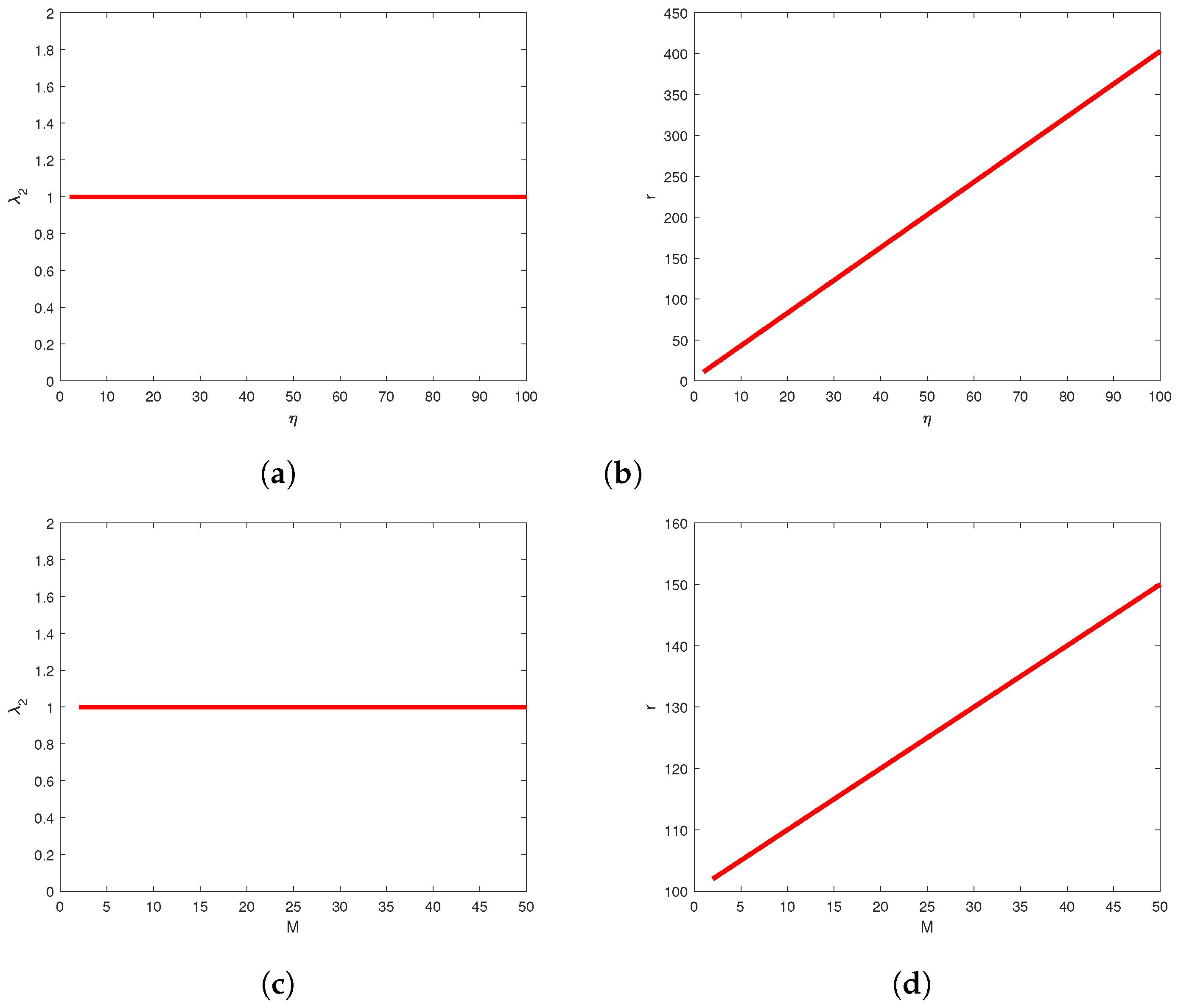
Let $a=2,d=1,M=2$, the relationship between the number of leaves $\eta$ and the synchronizability of Networks-A is shown in Figure 5a,b. Because each layer has N nodes, satisfying $N=2\eta +1$, we can plot ${\lambda }_2$ and r changing with $\eta$ to analyze the impact of the number of leaves $\eta$ on network synchronizability. From Figure 5a, when talking about the unbounded synchronized region, it is clear that the value of ${\lambda }_2$ remains invariant with the increase of $\eta$. This indicates that the network size N does not take into account the synchronizability of Networks-A. Figure 5b shows that the synchronizability, the bounded synchronized region, is weakened because r increases as $\eta$ increases.

(4)

Let $a=2,d=1,\eta =50$, the relationship between the value of M and the synchronizability is shown in Figure 5c,d. In the unbounded synchronized region, ${\lambda }_2$ of the supra-Laplacian matrix does not change with the increase of M which means that the capacity of synchronization is unaffected by the number of layers. In the bounded synchronized region, the value of r increases and the network synchronizability is eroded when M increases from 2 to 50, indicating that synchronizability is diminished as the layers increases.

4.2. The Synchronizability of Networks-B

(1)

Let $M=2,\eta =100,d=1$. Figure 6a,b show the variation of ${\lambda }_2$ and r relative to different values of the intra-layer coupling strength a. For the unbounded synchronized region, it clearly shows that the value of ${\lambda }_2$ increases linearly at first with a ($a<a^{*}=2d$ ), and then remains invariant at ${\lambda }_2=2$ ($a\ge a^{*}$). This implies that the synchronizability of Networks-B is first strengthened and then holds constant with the increase of intra-layer coupling strength a. For the unbounded synchronized region, panel (b) shows that the value of r firstly decreases slowly and indicates that the synchronizability of Networks-B is enlarged when $a<a^{*}$. It increases monotonically when $a>a^{*}$, representing the capacity becoming weaker. The synchronizability, reaching the optimum with the increase of a, is maximized at $a^{*}=Md=2$.

(2)

Let $M=2,\eta =100,a=1$, the influence of the inter-layer coupling strength d on the synchronizability of Networks-B is display in Figure 6c,d. When d increases from 0 to 0.5 ($d\le d^{*}$), the smallest nonzero eigenvalue ${\lambda }_2$ increases, the eigenratio r decreases sharply, and the network synchronizability is strengthened. When d increases from 0.5 to 5 ($d>d^{*}$), ${\lambda }_2$ remains a fixed value at 1 means that the capability of synchronization is not influenced by d. While r increases slightly showing a weakening in synchronizability of intra-layer directed networks. The optimal solution of Networks-B is derived at $d^{*}=a/2=0.5$.

(3)

Let $a=0.5,d=1,M=2,\eta \ge 4$. In the case of the unbounded synchronized region, panel (a) in Figure 7 shows that the value of ${\lambda }_2$ does not vary with the increase of $\eta$, which indicates that the number of nodes N does not show any effect on the synchronization ability of Networks-B. In the bounded synchronized region, panel (b) shows that the synchronizability is weakened because r becomes larger when $\eta$ changes from 1 to 100.

(4)

Let $a=1,d=0.1,\eta =50$. Unlike the analysis result of Networks-A for the number of layers, panel (c) shows that ${\lambda }_2$ monotonically increases from 0.2 to 1, and then keeps invariant at 1. panel (d) shows that the eigenratio r, determined with ${\lambda }_{max}$ and ${\lambda }_2$, decreases and then increases slightly when the number M changes from 2 to 50.

4.3. The Synchronizability of Networks-C

According to the numerical examples shown in Figure 8 and Figure 9, the synchronizability of Networks-C changing with the increasing network parameters is similar to Networks-A. In the case of the unbounded synchronized region, ${\lambda }_2$ increases firstly and then transforms into a constant value whether with the intra-layer linking intensity a or the inter-layer linking intensity d. This property that the synchronizability of multilayer networks first increases and then remains constant is reflected in the figures. For the number of leaves $\eta$ within each layer and the number of layers M, ${\lambda }_2$ remains constant. This means that the synchronization capacity always remains a constant when the network size tends to infinity. In other words, in the case of the bounded synchronized region, the value of r, decreasing firstly and then increasing slightly whether for a or d, represents the evolution of synchronization capacity. When talking about the bounded synchronized region the synchronizability for this particular network is enhanced firstly, and then is diminished after achieving the optimum. For $\eta$ and M, the value of r increases linearly which means that the network synchronizability gets weaker as the network size increases.

5. Conclusions

This paper examined the synchronizability for multilayer directed Dutch windmill networks. The analytical expressions for all eigenvalues of the three networks have been rigorously derived and specific relations of synchronizability are given in Table 1, Table 2 and Table 3 that have been well verified by numerical simulation. By varying a single parameter, we discussed the impacts of the intra-layer coupling weights a, the inter-layer coupling weights d, network size N as well as the number of layers M on network synchronizability.

The effects of changes in all structure parameters upon the network synchronizability for Networks-A and Networks-C are similar. When taking into account the synchronization region with unbounded range, there are only two coupling weights a and d have remarkable influence on the synchronizability of Networks-A and Networks-C. However, for Networks-B, not only the coupling strength but also the number of layers have an influence on the synchronizability of the network. When taking into account the synchronization region with bounded range, the fewer nodes, the better the synchronizability. In addition, we would further discuss methods to improve or weaken the synchronization of multilayer directed networks in order to control the synchronization phenomenon in real life. There are still many problems to be solved in directed Dutch windmill networks. For example, when the strength of inter-layer coupling between central nodes differs from the strength of coupling between leaf nodes, we can study the change of synchronizability. Recently, the diffusion and coherence of networks are challenging and attractive topics, which are worthy of our further study of multilayer directed windmill networks.

References

- Watts, D.J.; Strogatz, S.H. Collective dynamics of ‘small-world’networks. Nature 1998, 393, 440–442. [Google Scholar] [CrossRef] [PubMed]
- Barabási, A.L.; Albert, R. Emergence of scaling in random networks. Science 1999, 286, 509–512. [Google Scholar] [CrossRef] [PubMed]
- Buldyrev, S.V.; Parshani, R.; Paul, G.; Stanley, H.E.; Havlin, S. Catastrophic cascade of failures in interdependent networks. Nature 2010, 464, 1025–1028. [Google Scholar] [CrossRef] [PubMed]
- Borgatti, S.P.; Mehra, A.; Brass, D.J.; Labianca, G. Network analysis in the social sciences. Science 2009, 323, 892–895. [Google Scholar] [CrossRef] [PubMed]
- Granell, C.; Gómez, S.; Arenas, A. Dynamical Interplay between Awareness and Epidemic Spreading in Multiplex Networks. Phys. Rev. Lett. 2013, 111, 128701. [Google Scholar] [CrossRef]
- Wu, X.; Li, Y.N.; Wei, J.; Zhao, J.; Feng, J.; Lu, J.A. Inter-layer synchronization in two-layer networks via variable substitution control. J. Frankl. Inst. 2020, 357, 2371–2387. [Google Scholar] [CrossRef]
- Xiao, J.; Zeng, Z.G.; Wen, S.P.; Wu, A.L.; Wang, L.M. Finite-/fixed-time synchronization of delayed coupled discontinuous neural networks with unified control schemes. IEEE Trans. Neural Netw. Learn. Syst. 2020, 32, 2535–2546. [Google Scholar] [CrossRef]
- Newman, M. Networks: An Introduction, 1st ed.; Oxford University Press: Oxford, MI, USA, 2010. [Google Scholar]
- Bianconi, G. Multilayer Networks: Structure and Function, 1st ed.; Oxford University Press: Oxford, MI, USA, 2018. [Google Scholar]
- Wang, S.; Zheng, S.; Cui, L. Finite-Time Projective Synchronization and Parameter Identification of Fractional-Order Complex Networks with Unknown External Disturbances. Fractal Fract. 2022, 6, 298. [Google Scholar] [CrossRef]
- Qi, F.; Qu, J.; Chai, Y.; Chen, L.; Lopes, A.M. Synchronization of incommensurate fractional-order chaotic systems based on linear feedback control. Fractal Fract. 2022, 6, 221. [Google Scholar] [CrossRef]
- Wei, J.; Wu, X.; Lu, J.A.; Wei, X. Synchronizability of duplex regular networks. EPL (Europhys. Lett.) 2018, 120, 20005. [Google Scholar] [CrossRef]
- Wei, X.; Emenheiser, J.; Wu, X.; Lu, J.A.; D’Souza, R.M. Maximizing synchronizability of duplex networks. Chaos Interdiscip. J. Nonlinear Sci. 2018, 28, 013110. [Google Scholar] [CrossRef] [PubMed]
- Wei, X.; Wu, X.; Lu, J.A.; Wei, J.; Zhao, J.; Wang, Y. Synchronizability of two-layer correlation networks. Chaos Interdiscip. J. Nonlinear Sci. 2021, 31, 103124. [Google Scholar] [CrossRef] [PubMed]
- Gomez, S.; Diaz-Guilera, A.; Gomez-Gardenes, J.; Perez-Vicente, C.J.; Moreno, Y.; Arenas, A. Diffusion dynamics on multiplex networks. Phys. Rev. Lett. 2013, 110, 028701. [Google Scholar] [CrossRef] [PubMed]
- Yu, Q.; Yu, Z.; Ma, D. A multiplex network perspective of innovation diffusion: An information-behavior framework. IEEE Access 2020, 8, 36427–36440. [Google Scholar] [CrossRef]
- Yan, H.; Zhou, J.; Li, W.; Lu, J.A.; Fan, R. Superdiffusion criteria on duplex networks. Chaos Interdiscip. J. Nonlinear Sci. 2021, 31, 073108. [Google Scholar] [CrossRef]
- Hu, T.; Li, L.; Wu, Y.; Sun, W. Consensus dynamics in noisy trees with given parameters. Mod. Phys. Lett. B 2022, 36, 2150608. [Google Scholar] [CrossRef]
- Hong, M.D.; Sun, W.G.; Liu, S.Y.; Xuan, T.F. Coherence analysis and Laplacian energy of recursive trees with controlled initial states. Front. Inf. Technol. Electron. Eng. 2020, 21, 931–938. [Google Scholar] [CrossRef]
- Li, Y.; Zhong, J.; Lu, J.; Wang, Z.; Alssadi, F.E. On robust synchronization of drive-response Boolean control networks with disturbances. Math. Probl. Eng. 2018, 2018, 1737685. [Google Scholar] [CrossRef]
- Leyva, I.; Sevilla-Escoboza, R.; Sendiña-Nadal, I.; Gutiérrez, R.; Buldú, J.; Boccaletti, S. Inter-layer synchronization in non-identical multi-layer networks. Sci. Rep. 2017, 7, 45475. [Google Scholar] [CrossRef]
- Yu, W.; Lu, J.; Yu, X.; Chen, G. Distributed adaptive control for synchronization in directed complex networks. SIAM J. Control Optim. 2015, 53, 2980–3005. [Google Scholar] [CrossRef]
- Wang, Y.W.; Bian, T.; Xiao, J.W.; Wen, C. Global synchronization of complex dynamical networks through digital communication with limited data rate. IEEE Trans. Neural Netw. Learn. Syst. 2015, 26, 2487–2499. [Google Scholar] [CrossRef] [PubMed]
- Wang, L.M.; Jiang, S.; Ge, M.F.; Hu, C.; Hu, J.H. Finite-/fixed-time synchronization of memristor chaotic systems and image encryption application. IEEE Trans. Circuits Syst. Regul. Pap. 2021, 68, 4957–4969. [Google Scholar] [CrossRef]
- Fan, C.X.; Jiang, G.P.; Jiang, F.H. Synchronization between two complex dynamical networks using scalar signals under pinning control. IEEE Trans. Circuits Syst. Regul. Pap. 2010, 57, 2991–2998. [Google Scholar] [CrossRef]
- Xu, M.M.; Lu, J.A.; Zhou, J. Synchronizability and eigenvalues of two-layer star networks. Acta Phys. Sin. 2016, 65, 028902. [Google Scholar]
- Zhang, L.; Wu, Y.Q. Synchronizability of Multilayer networks With K-nearest-neighbor Topologies. Front. Phys. 2020, 8, 571507. [Google Scholar] [CrossRef]
- Li, J.; Luan, Y.; Wu, X.; Lu, J.A. Synchronizability of double-layer dumbbell networks. Chaos Interdiscip. J. Nonlinear Sci. 2021, 31, 073101. [Google Scholar] [CrossRef]
- Kanna, M.R.; Kumar, R.P.; Jagadeesh, R. Computation of topological indices of Dutch windmill graph. Open J. Discret. Math. 2016, 6, 74–81. [Google Scholar] [CrossRef]
- Estrada, E. When local and global clustering of networks diverge. Linear Algebra Appl. 2016, 488, 249–263. [Google Scholar] [CrossRef]
- Kooij, R. On generalized windmill graphs. Linear Algebra Appl. 2019, 565, 25–46. [Google Scholar] [CrossRef]
- Sun, W.; Li, Y.; Liu, S. Noisy consensus dynamics in windmill-type graphs. Chaos Interdiscip. J. Nonlinear Sci. 2020, 30, 123131. [Google Scholar] [CrossRef]
- Zhu, J.; Huang, D.; Jiang, H.; Bian, J.; Yu, Z. Synchronizability of multi-layer variable coupling windmill-type networks. Mathematics 2021, 9, 2721. [Google Scholar] [CrossRef]
- Tang, L.; Wu, X.; Lü, J.; Lu, J.A.; D’Souza, R.M. Master stability functions for complete, intralayer, and interlayer synchronization in multiplex networks of coupled Rössler oscillators. Phys. Rev. E 2019, 99, 012304. [Google Scholar] [CrossRef] [PubMed]
- Zhang, S.; Wu, X.; Lu, J.A.; Feng, H.; Lü, J. Recovering structures of complex dynamical networks based on generalized outer synchronization. IEEE Trans. Circuits Syst. Regul. Pap. 2014, 61, 3216–3224. [Google Scholar] [CrossRef]
- Sole-Ribalta, A.; De Domenico, M.; Kouvaris, N.E.; Diaz-Guilera, A.; Gomez, S.; Arenas, A. Spectral properties of the Laplacian of multiplex networks. Phys. Rev. E 2013, 88, 032807. [Google Scholar] [CrossRef] [PubMed]
- Wang, X.F.; Li, X.; Chen, G.R. Network Science: An Introduction, 1st ed.; High Education Press: Beijing, China, 2012. (In Chinese) [Google Scholar]
- Gallian, J.A. A survey: Recent results, conjectures, and open problems in labeling graphs. J. Graph Theory 1989, 13, 491–504. [Google Scholar] [CrossRef]
- Horn, R.A.; Johnson, C.R. Matrix Analysis, 2nd ed.; Cambridge University Press: New York, NY, USA, 2013. [Google Scholar]
- Deng, Y.; Jia, Z.; Yang, F. Synchronizability of multilayer star and star-ring networks. Discret. Dyn. Nat. Soc. 2020, 2020, 9143917. [Google Scholar] [CrossRef]
Figure 1.
Schematic diagram of multilayer directed Dutch windmill networks. (a) Networks-A with two layers; (b) Networks-B with two layers; (c) Networks-C with two layers.
Figure 2.
Structure schematic diagram of Networks-A with M layers.
Figure 3.
State trajectories of the two-layer Networks-C with 7 nodes in each layer. The trajectories of the first layer are plotted as red dashed lines, and the trajectories of the second layer are plotted as blue solid lines.
Figure 4.
The synchronizability of Networks-A. Panel (a) depicts vs. a and (b) depicts r vs. a when ; Panel (c) depicts vs. d and (d) depicts r vs. d when .
Figure 5.
The synchronizability of Networks-A. Panel (a) depicts vs. and (b) depicts r vs. when ; Panel (c) depicts vs. M and (d) depicts r vs M when .
Figure 6.
The synchronizability of Networks-B. Panel (a) depicts vs. a and (b) depicts r vs. a when ; Panel (c) depicts vs. d and (d) depicts r vs. d when .
Figure 7.
The synchronizability of Networks-B. Panel (a) depicts vs. and (b) depicts r vs. when ; Panel (c) depicts vs. M and (d) depicts r vs. M when .
Figure 8.
The synchronizability of Networks-C. Panel (a) depicts vs. a and (b) depicts r vs. a when ; Panel (c) depicts vs. d and (d) depicts r vs. d when .
Figure 9.
The synchronizability of Networks-C. Panel (a) depicts vs. and (b) depicts r vs. when ; Panel (c) depicts vs. M and (d) depicts r vs. M when .